Abstract
Electric drive control is an important area of research due to its ubiquity. In particular, multi-phase induction machines are an important field due to their inherent robustness. Tuning of the inner loop (speed) and outer loop (current) is typically tackled separately. The problem of trade-off analysis for the tuning of both loops has never been tackled before, which motivates the present study. This paper examines the complex and non-linear relationships between commonly used performance indicators in variable speed applications. The paper shows that there are links between performance indicators for both loops. This prompts a more detailed study of concurrent tuning. Also, it is shown that said links are, in a variable speed drive, dependent on the operating point. This requires studying more than just one operating point. Experimental results for a five-phase induction motor are used to validate the analysis.
1. Introduction
Today’s state-of-the-art control of Induction Machines (IM) uses a double-loop scheme consisting of an inner loop for current and an outer one for speed. Speed control uses, in most cases, a Proportional-Integral (PI) scheme. The PI output is the current/torque reference for the inner control loop. There, stator currents must be produced by the power converter to meet the reference value. Discrete techniques such as Pulse Width Modulation (PWM) are typically used to drive the power converter. One interesting spin-off appears when the inner control loop is replaced by direct digital predictive control of the discrete states of the power converter. The resulting scheme has been referred to as Finite State Model Predictive Control (FSMPC). This method has been applied to many different types of motors including the multi-phase induction motor [1]. The technique is of importance for many applications, but especially for multi-phase systems, where the increased number of phases makes the design of controllers difficult. The flexibility of FSMPC allows easy treatment of a different number of phases as well as different control objectives [2].
The Multi-phase IM features low torque ripple, reduced harmonics, high reliability and enhanced power distribution per phase [3]. However, a large number of switching states must be dealt with [4]. The recent apparition of fast predictive controllers [5] has made this obstacle less important. However, managing the different objectives is still an open problem. Although past works have considered a subset of objectives (for instance tracking vs. regulation), the number of different performance indicators (electric, electronic, mechanical) is large and this has created a research opportunity still to be explored in full.
The state of the art regarding trade-offs for variable speed drives include early efforts concerned with tuning the Cost Function (CF) of FSMPC [6]. The CF is used at each sampling period to derive the control signal. As a result, some performance indicators are, to some extent, influenced by the terms present at the CF. Weighting Factors (WF) are used to balance the relative importance of said terms. Early papers about FSMPC have dealt with WF tuning [7], concluding that a particular compromise solution has to be found since objectives collide with each other [8]. This was first exposed in [9], where a reduced set of variables was used for assessment. Similarly, in [10], the impossibility of improving all figures of merit at once is realized with the help of a Pareto diagram for a six-phase machine. This realization prompted researchers to develop methods for CF tuning. For instance, in [2] soft constraints are utilized for a nine-phase IM. However, this proposal does not tackle the issue of dependency on the operating condition. The tuning method of [10] is not adaptive, but different figures of merit and different operating points are considered. Similarly, in [11], different operating points are used to define a scheduled solution. In [12], the switching frequency is considered using neural networks to provide inter-sample modulation in a multi-vector approach. A similar work is presented in [13] but resorting to physical considerations about the sequence of control actions. Other indicators have also been considered, such as common-model voltage [14]. However, in none of the above, are the trade-offs arising when considering both loops studied.
Considering other applications besides drives, a Lyapunov-based design is proposed in [15] for a dual-output multilevel rectifier. In [16], an extra term is used to balance the neutral point voltage of a multilevel inverter. Tuning of the resulting CF is achieved using the Vikor decision method on the Pareto front. Many more methods have been proposed for electrical systems that do not drive. These are not considered here since a drive has more complex dynamics. In particular, the effect of speed is absent in converter-supplied loads. This effect must be considered for variable-speed drives.
Continuing with WF tuning, some researchers have proposed methods for WF elimination [17]. Other authors, however, take the WF as degrees of freedom to tune their FSMPC to their particular applications [18]. A model reference tuning method is used in [19] for the FSMPC of a six-phase machine not considering the speed loop. In [20] a fuzzy adaptive control and weighting factor to reduce the speed, torque and flux ripples is proposed. The method is tested by simulations and hardware-in-loop. Also, speed is considered but load is not. The contribution is nevertheless interesting as different figures of merit are considered, unlike in previous works.
1.1. Motivation
In light of the previous discussion, an analysis of trade-offs between performance indicators is in order. The analysis must include electric, electronic and mechanical variables. The lack of such study in the literature constitutes the main motivation for this study. Please notice that even considering just one of the loops (speed or current), there are few papers concerned with trade-off analysis [21].
Regarding speed control, a typical research work, such as [22], presents PI tuning laws using some technique such as fuzzy inference. More often than not, just one or two mechanical performance indicators are used. Other works such as [23] use different mechanical performance indicators as part of some optimization. In [24], the influence of hyper-parameters for a PID tuner is presented. The work deals with Single Input Single Output processes, but considers various performance indicators, obtaining trade-offs as a consequence. This type of methodology has been applied to different systems where speed control is in order and especially in those using fuzzy and/or neural approximations [25]. After this, some papers have dealt with improving mechanical response while considering the predictive inner controller. For instance, mechanical speed overshoot is reduced in [26] by means of a radial basis function controller for a permanent magnet motor. In all cases, trade-offs are neither highlighted nor analyzed. An example of trade-off analysis is found in the field of electric vehicles [27], where energy is considered. However, this variable is not directly manipulable.
Regarding the inner loop for current stator control, the seminal work of [9] showed the trade-offs for CF tuning in multi-phase systems. Similar ideas were explored in [10,28] with the help of a Pareto analysis. The work of [29] presents a disturbance observer for a terminal sliding mode speed controller. An adaptive tuning is used for the WF. In both cases, a permanent magnet system is considered. This is due in part to the simplified dynamics compared with a multi-phase induction motor. The concurrent tuning of both loops has not been tackled in any of the above.
1.2. Novelty and Contributions
From the above analysis of the existing literature, it is clear that the problem of trade-off analysis for the tuning of both loops for multi-phase IM has never been solved before. Therefore, the originality and novelty of this paper lie in the fact that said analysis has finally been done. It will be shown that such an analysis casts some light on the problem that can be used to guide future research. The study is important as new tuning methods can not possibly succeed without a deep understanding of the trade-offs. The paper will show that the concurrent tuning of inner (FSMPC) and outer (PI) loops in the drive must be considered. This has not yet appeared in the literature. In this regard, the present study identifies a future research direction in the control of variable-speed drives. The following is a list of the contributions of the paper:
- Establishing links between performance indicators of different kinds: electric, electronic, and mechanic.
- Tackling the concurrent tuning of the inner and outer loops of a variable speed drive.
- Providing evidence for the existence of complex relationships between mechanical and electrical indicators.
- Highlighting the importance of the mechanical operating point in the analysis.
The rest of the paper is organized as follows: Section 2 introduces the problem formulation and the necessary theoretical background for the analysis. This is conducted in Section 3 with the help of experiments in a laboratory setup. Finally, the discussion in Section 4 extracts the main conclusions of the study.
2. Background on FSMPC Drive Control
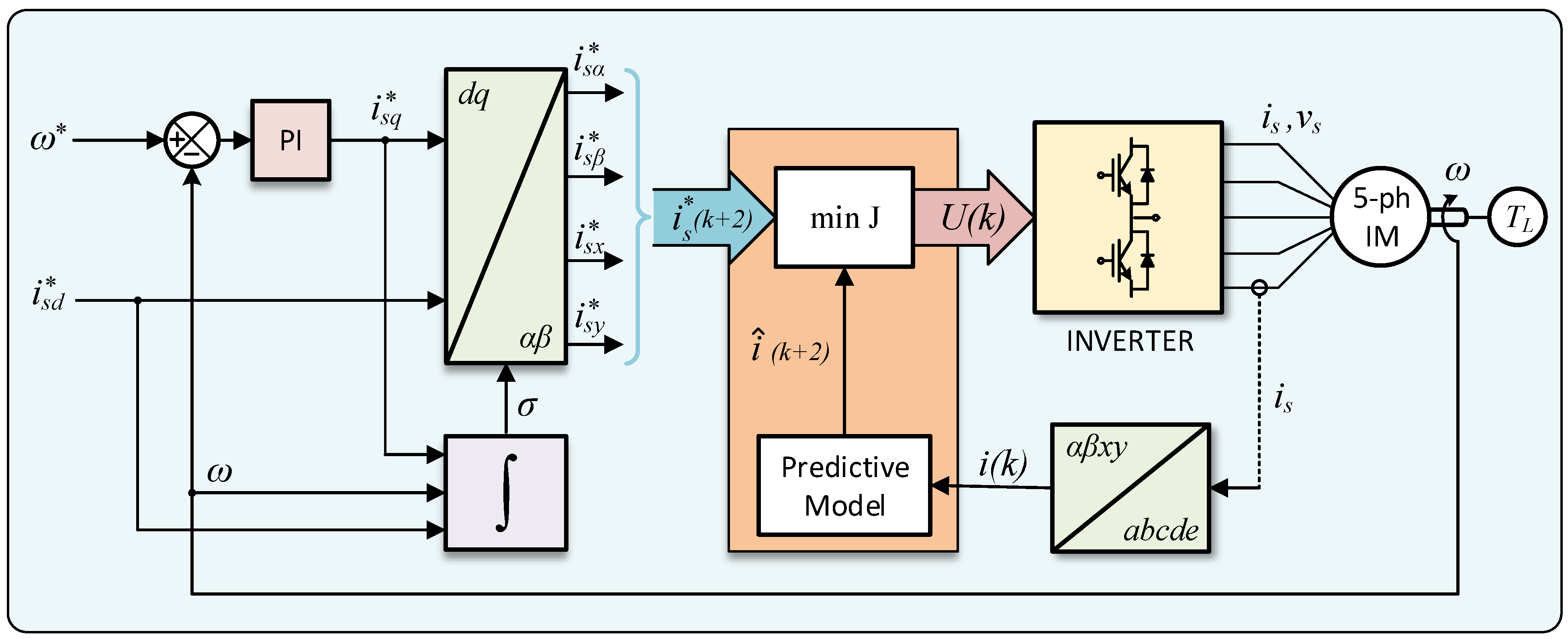
The fundamentals of FSMPC drive control can be reviewed with the help of Figure 1. The particular case of five phases is considered for concreteness. The main elements are the speed PI controller, the stator current controller, the five-phase converter and the five-phase IM.
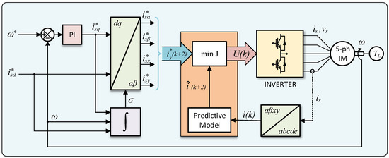
Figure 1.
Diagram of the PI+FSMPC control method for a five-phase IM drive.
In FSMPC, the aim is to drive stator currents to a desired reference in order to produce an adequate amount of torque. This torque will keep the machine rotating at the desired speed . The stator currents are managed by the FSMPC by providing different phase voltages. These voltages are produced by the Voltage Source Inverter (VSI). A five-phase VSI can sustain configurations resulting from the discrete states of its switches. The state (on/off) of the upper switch of the leg is denoted as . Vector constitutes the control action (input signal) of the FSMPC scheme. It is possible to compute the stator phase voltages as , where , and T is the following connectivity matrix
In (1), the quantity is the DC-link voltage. Instead of phase quantities, it is more common to use a vector space decomposition projecting phases into two planes. Assuming distributed windings, the first plane () produces flux and torque, and the other () just contributes to losses. The transformation matrix is
where , , and (rad). Quantities in are obtained as .
The reference for stator current in coordinates are obtained in a way similar to that of the Indirect Field Oriented Control (IFOC) scheme. There, quantities in the rotating reference frame are used to link the speed-PI output to electrical variables. Recall that the d component deals with flux production and the q component with torque. The Park rotation matrix is then used to convert the axes into , so , with
where the flux position is obtained as . The angle estimation procedure uses the measured mechanical speed to compute the electrical angle , being P the number of pairs of poles of the IM and the IM slip [30].
The stator currents are given a reference value by the speed-loop PI. This value is represented as . The d component is fixed to produce a constant flux, and the q component produces torque to drive the mechanical speed control error to zero and is computed as
where and are proportional and integral gain factors, respectively, is the velocity error and is the mechanical speed reference.
The value must be transformed to for stator current control, resulting in , , , with .
The FSMPC part is responsible for stator current tracking of . For this, a model-based scheme is used where the control action U is determined to minimize a CF. The CF contains some terms related to deviations in the control objectives. These terms are predictions provided by the machine model. It is thus convenient to write the model as the one-step-ahead prediction in stator currents
where and are the matrices of the model.
In order to cope with the delay in computations a second prediction is used. This is obtained as . Penalties are placed on predicted control errors and the number of switch changes, resulting in
where is the quadratic deviation of predictions from the reference in the plane, is the quadratic deviation of predictions from a reference in the plane, and are weighting factors and is the number of switch changes in the VSI:
The overall scheme (as indicated in Figure 1) consists of translating the speed reference to stator current references that are handled by the predictive scheme. Then the control action for () is computed at discrete time k minimizing the CF.
2.1. Control Objectives
Depending on the application for the drive, different control objectives can be established. For instance, in some applications overshooting is very important and other objectives such as rise time receive less attention, in others, it could be the opposite. The trade-off analysis should consider a subset of control objectives that are, for the most part, independent of each other.
For the sake of concretion, in this paper, the performance indicators considered include the mechanical, electromagnetic and electronic variables listed and defined below. Each indicator is given a number i, so that it can be referred to as .
- Overshoot in mechanical speed (), Equation (8). Most applications tolerate a certain amount of overshoot, nevertheless a low value is sought after in most cases.
- Rise time of mechanical speed (), Equation (9). In over-damped systems, it is measured as the time needed to cover 90 % of the reference step. In under-damped systems, it is the time needed to reach the new reference. A low value is required in most applications.
- Integral Time Absolute Error () is a measure of tracking error that penalizes long-lasting errors more than initial transient ones as defined in Equation (10).
- Torque ripple (), Equation (11). This variable has an electro-magnetic origin as the produced torque and is directly defined by stator currents. At the same time, with torque as the driving force of the motor, torque ripple has an effect on speed. In fact, torque ripple can cause mechanical stress in the axis and so must be reduced.
- Harmonic content (), Equation (12) is an electrical variable that measures how much inefficiency is due to subspace content. The factor is used in the CF as a means to reduce currents.
- Average switching frequency (), Equation (13) is a measure of how often the VSI is changing the state of its switches. It must be kept within appropriate values depending on the VSI technology. The factor is introduced in the cost function precisely to reduce commutation frequency.
Mathematical definitions of the performance indicators are provided in the following.
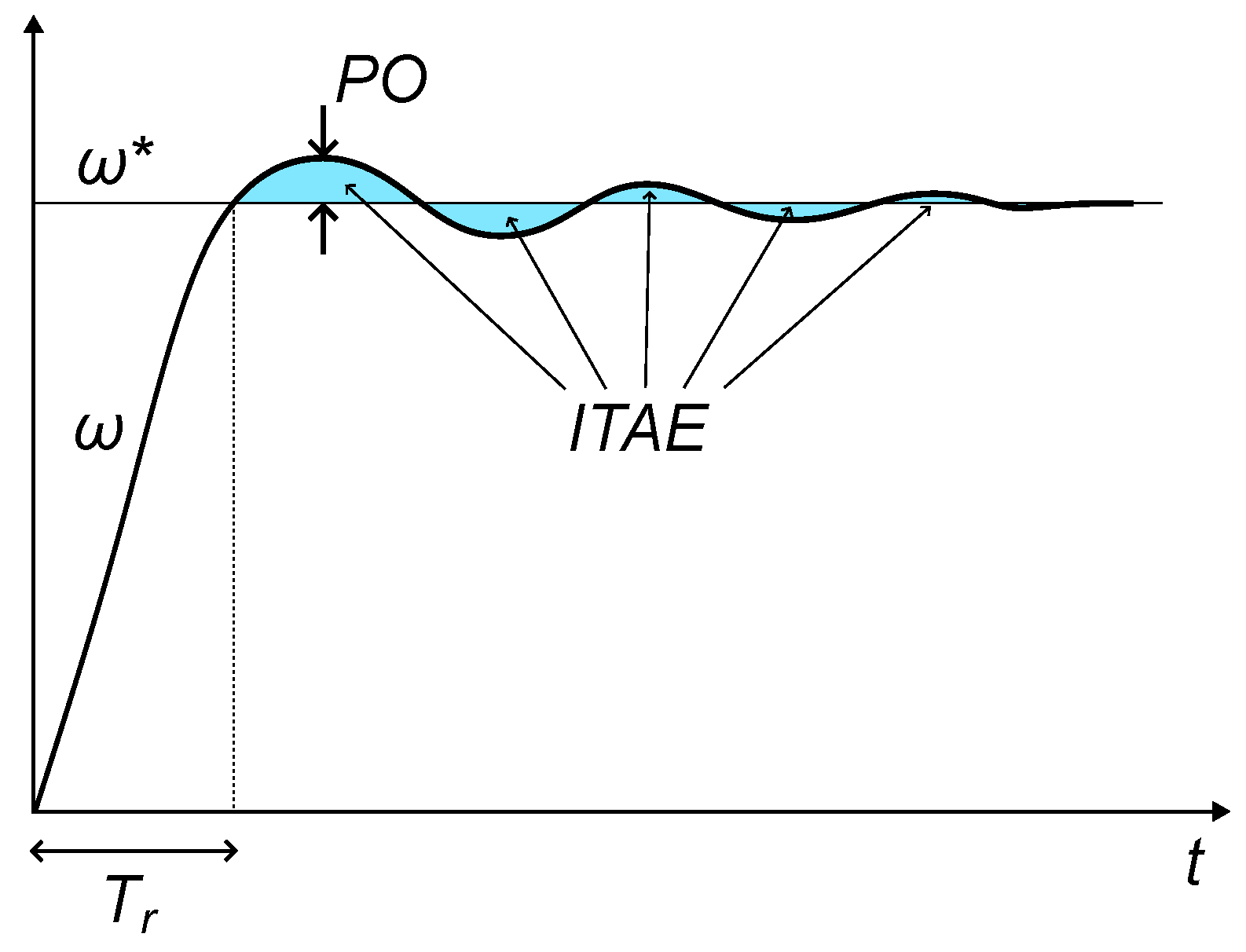
As a reminder of control concepts, Figure 2 shows the trajectories for several variables during a step test. The different values are identified in the graphs. Please notice that all indicators considered here can be found in basic literature about variable-speed drives [31].
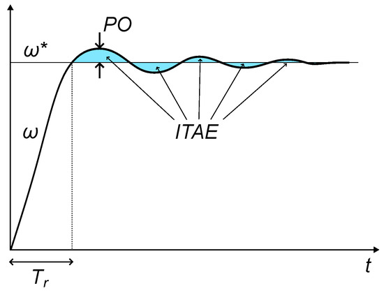
Figure 2.
Illustration of the performance indices , and .
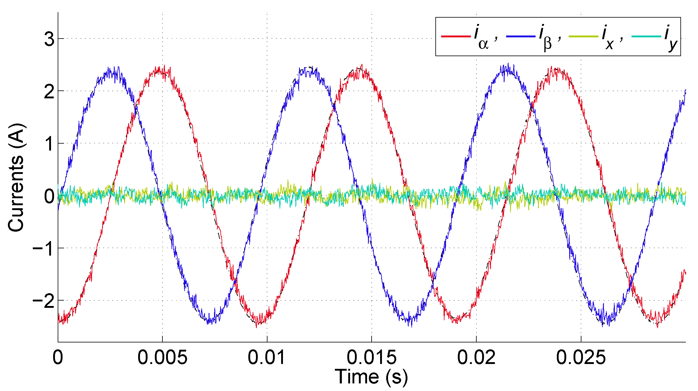
Also, regarding electrical variables and their associated performance indicators, Figure 3 presents a waveform of and currents for and . Recall that these WF have an effect on and . For this particular case, (A) (about 2% of the rated current), (kHz). This latter value is of importance as it must fall in the supported range for the VSI to avoid damage to the semiconductor.
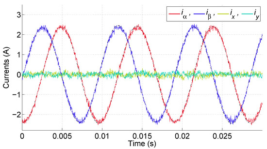
Figure 3.
Evolution of stator currents in and planes.
2.2. Cost Function Tuning
Tuning of the drive is usually performed using the two time-scales decomposition allowing for dealing independently with each loop. Regarding the inner loop, tuning the FSMPC consists of selecting the values for parameters and [1]. These parameters influence the selected control action on each sampling period, as a result, they influence the performance indices as will be shown later. The selection is usually conducted by trial and error, having as guidance discrete measurements on some performance indices. This can be conducted via simulation, actual experimentation, or a combination of the two [32].
The most widely reported difficulty with respect to CF tuning in FSMPC is that the influence of WF on performance indices is not linear, in fact, it is not even monotonic. This has been explored mainly in papers dealing with applications that are not drives.
Another difficulty of CF tuning, although many times not reported, lies in the fact that drives feature a non-linear dependence of performance indicators with respect to the actual operating point. Of course, this only appears in applications where operating points can clearly be defined as functions of some variables such as mechanical speed. This is the case with variable-speed drives. This prompted the authors to propose a CF tuning that is operating-point dependent [11].
Another difficulty stems from the trade-offs existing between performance indicators even for a fixed operating point. One would think that it would be desirable to minimize all simultaneously. However, the analysis to be presented in Section 3 shows that this is impossible. This is in line with previous findings by the authors [9] and others [10].
Also, it would be logical to think that performance indicators pertaining to one category (mechanical, electromagnetic, electronic) do not interfere with performance indicators of other categories. This paper shows that this intuition is not correct. As a result, the analysis must encompass not only CF tuning but also PI tuning in a unified fashion. To the best of our knowledge, this has not been conducted in a systematic way before [33].
2.3. Experimental Setup
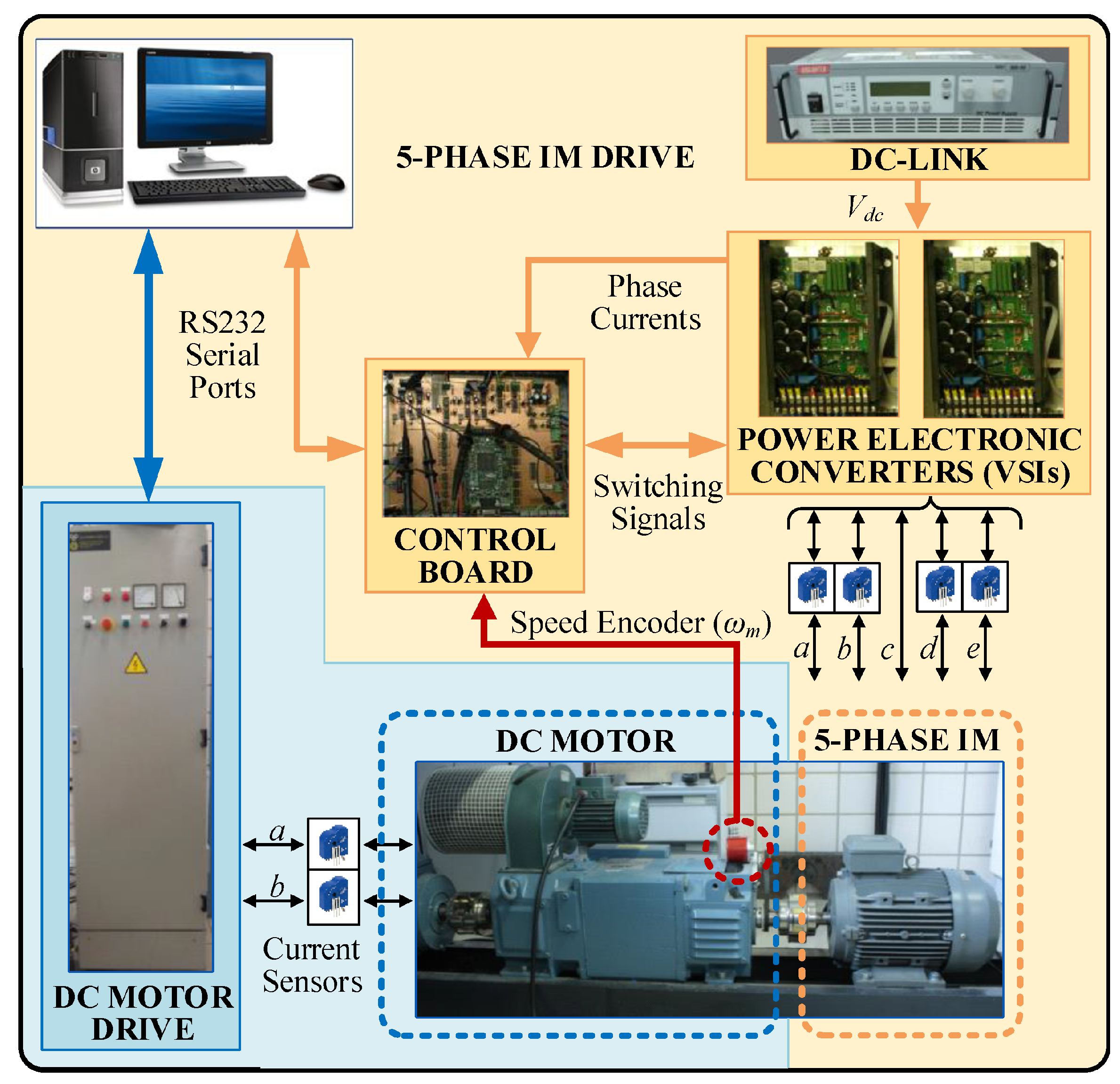
A laboratory system is used to validate the analysis with experiments performed on a real five-phase induction machine. The experimental setup includes (see Figure 4) a five-phase IM, with parameters shown in Table 1, a power converter using two SEMIKRON SKS 22F modules (SEMIKRON DANFOSS, Nürnberg, Germany). The VSI parameters are 22 (A) max. at 10 kHz with a max. of 15 (kHz). The VSI is powered by a 300 V DC power supply (Keysight, Colorado Springs, CO, USA). The control uses an MSK28335 board (Technosoft, Blue Ash, OH, USA) including a TMS320F28335 Digital Signal Processor (DSP) (Texas Instruments, Dallas, TX, USA), where the control program is run in real-time. The DC-link uses 300 (V) for a rated current 1.5 (A).
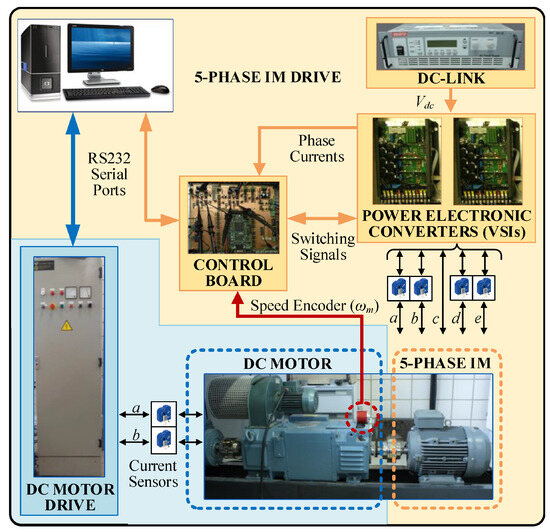
Figure 4.
Elements of the experimental five-phase IM drive.

Table 1.
Parameters of the Experimental five-phase IM.
The IFOC scheme of Figure 1 is used for the double-loop control. The mechanical speed is sensed using a GHM510296R/2500 encoder (Sensata Technologies, Attleboro, MA, USA). An interruption routine of the DSP is used to compute the mechanical speed from incoming encoder pulses. Regarding the inner control loop, Hall effect sensors (LH25-NP) (LEM, Meyrin, Switzerland) are used to measure the stator phase currents.
The setup has the ability to test the controller with some independence of the mechanical load characteristic curve thanks to a co-axial DC motor that is used to generate an independent opposing torque load () for the tests.
3. Trade-Off Analysis
The trade-off analysis is derived for a five-phase IM with FSMPC for current tracking and PI for speed tracking. The analysis considers all possible tunings to expose links between figures of merit. The methodology is explained in what follows.
3.1. Methodology
The methodology for the analysis consists of the following steps.
3.1.1. Research Design
The research design follows the usual steps in a control assessment project for variable-speed electrical drives. In particular, the realization of closed-loop experiments with a fixed value for control parameters. In these experiments, the manipulated and controlled variables are logged for later analysis.
3.1.2. Data Collection
- The performance indicators were then computed using (8)–(13) on the measured variables.
- The parameters of the PI and FSMPC were explored considering many different combinations of the WF of the CF and of the parameters of the PI.
- Performance maps were derived for the indicators as a function of the control parameters.
- The maps were then analyzed to draw conclusions that are valid for all possible tunings.
3.1.3. Analysis Method
The analysis was made by careful observation of the performance maps. There is no particular tool used for that. In particular, three types of conclusions were sought by the analysis: (a) the existence of links between performance indicators, (b) constraints introduced on the WF as a result of desired values for performance indicators and its importance for tuning, and (c) the influence of the operating point.
3.2. Analysis
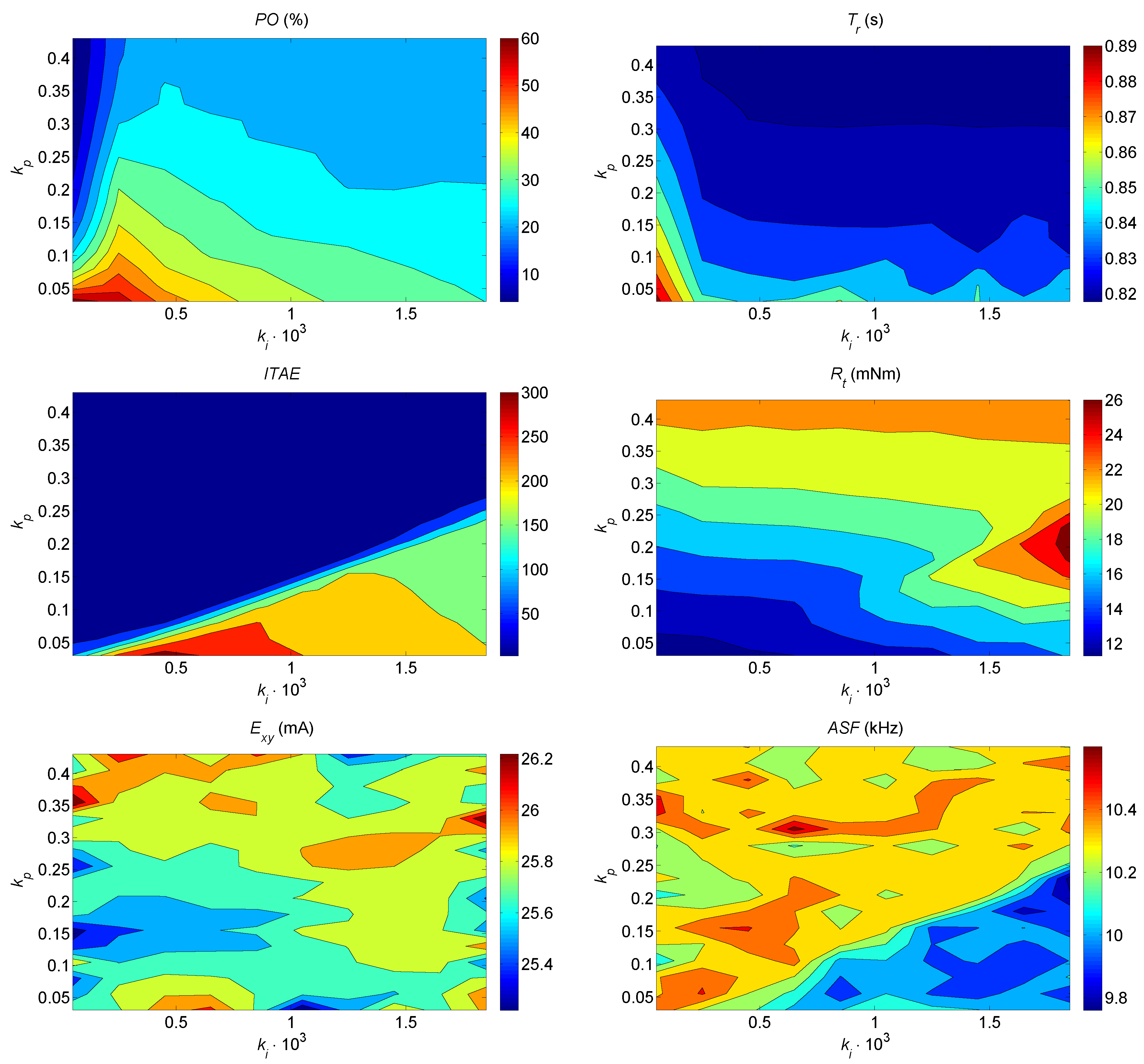
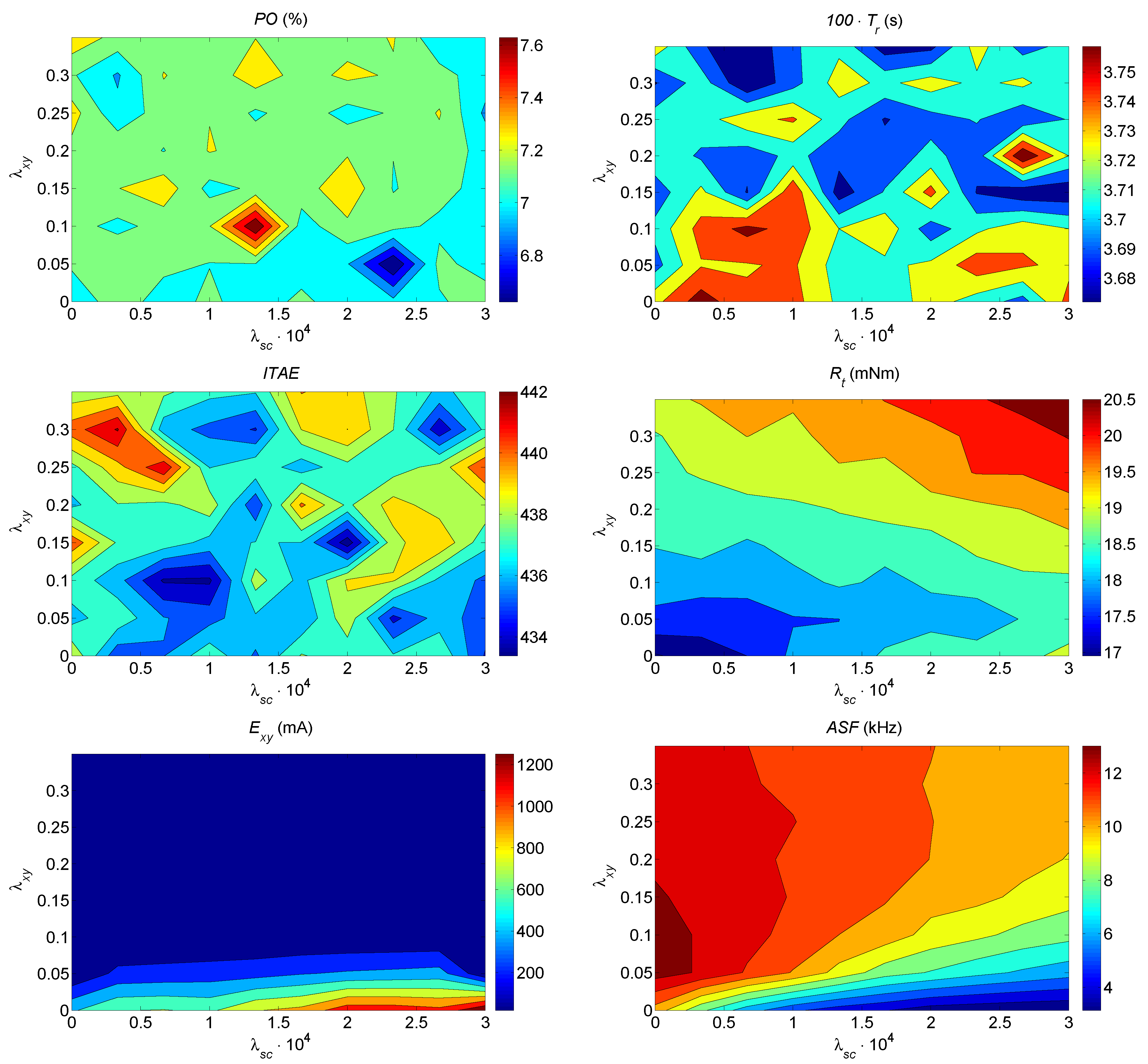
The first set of tests was performed using the following parameters: variable, variable, , , (s). The results are shown in Figure 5, where performance indices to are shown as contour plots for some , combinations. A number of useful observations can be made from these maps:
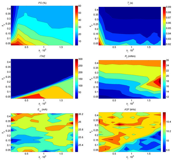
Figure 5.
Maps of the different performance indicators () in a - grid.
- The relationship between performance indices and controller parameters is non-linear. This is clearly seen for all performance indices as the contours are not straight lines.
- Minimizing all performance indices at once is not possible. This is clearly seen when comparing the values of and which have almost opposite behaviors. The , combinations that make low are around . However, for those parameters the value of is high. Similar trade-offs can be found for other combinations of performance indices for instance ASF and PO.
- Variables of different kinds are linked. This can be seen for instance considering values of and . The first variable is of the mechanical type, the second is of the electronic type affecting the power converter. The zone of low is the upper left corner, whereas the takes low values for the lower right corner. Similarly, connections between and and between and are clearly seen.
- From the map, it follows a clear dependence of on PI tuning. This means that hard constraints in cannot be satisfied independently of the outer PI configuration. This is an important fact that has not been previously reported. Recall that must be maintained below limits for risk of thermal damage to the power converter.
A second set of tests was performed using the following parameters: , , variable, variable, (s). The results are shown in Figure 6, where performance indices to are shown as contour plots for some and combinations. The following remarks can be made:
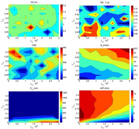
Figure 6.
Maps of the different performance indicators () in a - grid.
- The WF of the CF ( and ) cannot be set independently of each other. This is clearly seen in the maps of both and . For instance, a change in not only affects but also . The same happens with .
- The WF of the CF has a more noticeable effect on electrical/electronic variables ( and ) as expected; however, it also affects mechanical variables as can be clearly seen on the performance maps. This observation has not been reported before. The implications are of importance as this fact makes the tuning of the drive more challenging.
- It is interesting to see that the performance indicator acts as a link between purely mechanical variables (, , ) and electrical/electronic ones. This is also an interesting observation since most papers dealing with PI tuning in IFOC-like structures focus on mechanical variables alone. Conversely, papers dealing with converters do pay attention to but fail to connect it to mechanical variables.
3.3. Relevance for Tuning
The non-linear behavior and the trade-offs between performance indicators shown in the previous paragraphs carry out an important weight when it comes to controller tuning. It is important to remark that controller tuning is an active area of research. Even for the well-known PID controller, there are new proposals for tuning being made each year.
Of course, tuning must take into account the particular needs of each application. Here, for concretion’s sake, a typical scenario is used. In this scenario, two variables are given hard caps and the others are considered as trade-offs. The hard caps are imposed on and . The choice is motivated by the fact that most drives should avoid the oscillatory behavior imposed by high and by the fact that the power converter must work with under limits to avoid damage.
To work out an example, the following limits are chosen: (%), (kHz). From the map of Figure 5 it is clear that this restricts so that the selected lies in the upper-left corner of the map. Similarly, from the map of Figure 6, the restriction (kHz) leads to parameters being placed approximately under the main diagonal. With this in mind, tuning (A) shown in Table 2 aims at producing a under limits; however, the takes high values and is above limits. In order to reduce one can increase the integral action, which leads to tuning (B). It can be seen that is traded with . Incidentally, other performance indicators are affected, more notably is reduced and is increased. For tuning (C), the is taken into consideration. The value of is increased to reduce . As a result, a large increase in is observed as a main consequence. Tuning (D) tries to get below the established limits by means of an increase in . The consequences are an increase in and , but finally, the is under 10 (kHz).
Table 2.
Case examples illustrating the trade-offs.
3.4. Dependence on the Operating Point
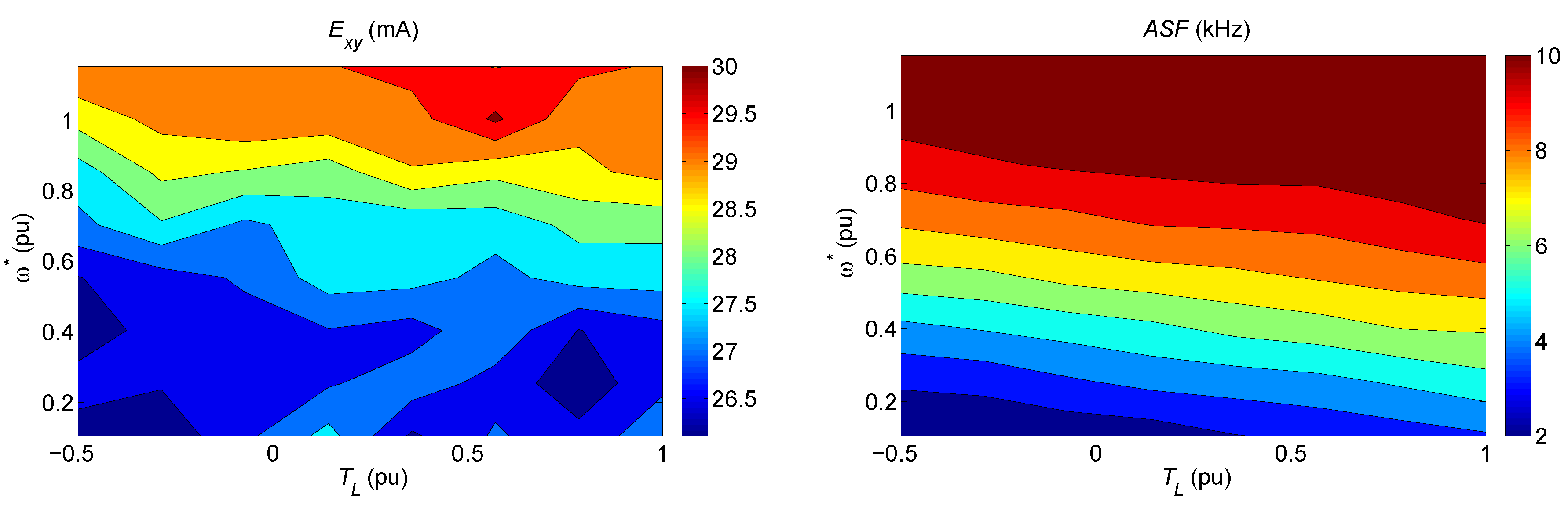
In the examples above, just a single operating point was considered. To obtain a complete picture of the complexity of the system, the effect of the operating point must be explored. In many variable-speed applications, the operating point is fixed by the speed. This is because the load is dependent on the speed through the mechanical characteristics. This is the case for pumps, compressors, fans, etc. In other cases, an opposing torque can appear independent of speed. This is the case of elevators, electric cars, conveyor belts, etc. The experimental setup shown in Figure 4 allows for the introduction of a torque load independent of speed, allowing the study of the dependence of the operating point on several figures of merit. The most striking results are how electrical variables are linked to speed and torque load. This is shown by the maps of Figure 7 where a constant tuning is used for all speed-load combinations. It can be seen that is quite sensitive to the operating point. This is rarely reported on in published works. The importance of this observation is two-fold. First, it demonstrates once again the link between electrical and mechanical variables in the drive. Second, it shows that, if a constant tuning is used, very different commutation rates are to be expected.
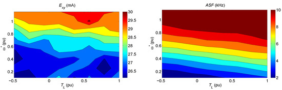
Figure 7.
Influence of mechanical operating point on electrical performance indicators.
4. Discussion
The results presented in the paper show several facts concerning the tuning of IM drives with FSMPC in the inner loop. These facts are often overlooked in published works.
- The links between variables of different kinds (mechanical, electrical, electronic) have been established thanks to the analysis of the performance maps. As a result, trade-offs appear involving different performance indicators of different types. The analysis has been made using maps for the indicators covering a wide range of tuning possibilities. The implication of this is that tuning alone cannot improve all performance indicators once the Pareto front has been reached. This should be taken into account when reporting improvements in the field.
- The concurrent tuning of inner (FSMPC) and outer (PI) loops in the drive is shown as an inevitable conclusion. Again, this has not yet appeared in the literature. In this regard, the present study presents a future research direction. In particular, the torque ripple appears as the main reason why both loops are linked. This can be seen in the performance maps. The implications of this are important as typical tuning does not consider both loops concurrently. This points in another direction for future research.
- The trade-off analysis shows that the usual practice of comparing one controller with another in a few scenarios is not thorough. The results shown here prompt a more complete assessment. Maps for different performance indicators should be provided. This observation should exist when reporting new controllers.
- The existence of complex relationships between mechanical and electrical indicators is a drawback for FSMPC because it makes tuning more complex than the case using PWM or any other modulation scheme where the switching frequency is constant. Whereas past works have deemed the tuning of FSMPC to be difficult, this analysis shows why.
- The operating point (in mechanical terms) has also been shown to influence electrical variables. Again, this fact is more often than not, not mentioned in the literature. Yet, it is of great importance for drives that must operate with different speeds and/or loads. The observation also points out a future line of research where the tuning is made dependent on the operating point.
Author Contributions
Conceptualization, all; methodology, M.G.S. and F.C.; software, M.G.S. and F.C.; validation, all; formal analysis and investigation, M.G.S. and F.C.; writing—original draft preparation, all; writing—review and editing, all; visualization, M.G.S. and J.M.M.-H.; supervision and funding acquisition, M.R.A. All authors have read and agreed to the published version of the manuscript.
Funding
This research is part of project I+D+i/PID2021- 125189OB- I00, funded by MCIN/AEI/ 10.13039/501100011033/ by “ERDF A way of making Europe”.
Data Availability Statement
The original contributions presented in the study are included in the article, further inquiries can be directed to the corresponding author.
Conflicts of Interest
The authors declare no conflicts of interest. The funders had no role in the design of the study; in the collection, analyses, or interpretation of data; in the writing of the manuscript; or in the decision to publish the results.
Abbreviations
The following abbreviations are used in this manuscript:
| ASF | Average Switching Frequency |
| CF | Cost Function |
| DSP | Digital Signal Processor |
| FS | Finite State |
| IFOC | Indirect Field Oriented Control |
| IM | Induction Machine |
| ITAE | integral of time-weighted absolute error |
| MPC | Model Predictive Control |
| PI | Proportional Integral |
| PO | Percentage Overshoot |
| PID | Proportional Integral Derivative |
| PWM | Pulse Width Modulation |
| VSI | Voltage Source Inverter |
| WF | Weighting Factor |
References
- Lim, C.S.; Levi, E.; Jones, M.; Rahim, N.; Hew, W.P. A Comparative Study of Synchronous Current Control Schemes Based on FCS-MPC and PI-PWM for a Two-Motor Three-Phase Drive. Ind. Electron. Trans. 2014, 61, 3867–3878. [Google Scholar] [CrossRef]
- Gonzalez-Prieto, I.; Zoric, I.; Duran, M.J.; Levi, E. Constrained model predictive control in nine-phase induction motor drives. IEEE Trans. Energy Convers. 2019, 34, 1881–1889. [Google Scholar] [CrossRef]
- Wang, Y.; Yang, J.; Yang, G.; Li, S.; Deng, R. Harmonic currents injection strategy with optimal air gap flux distribution for multiphase induction machine. IEEE Trans. Power Electron. 2020, 36, 1054–1064. [Google Scholar] [CrossRef]
- García Entrambasaguas, P.; González-Prieto, I.; Durán, M.; Bermúdez, M.; Barrero, F. Fault Tolerance in Direct Torque Control with Virtual Voltage Vectors. Rev. Iberoam. Autom. Inform. Ind. 2019, 16, 56–65. [Google Scholar] [CrossRef]
- Arahal, M.R.; Barrero, F.; Satué, M.G.; Bermudez, M. Fast Finite-State Predictive Current Control of Electric Drives. IEEE Access 2023, 11, 12821–12828. [Google Scholar] [CrossRef]
- Peng, J.; Yao, M. Overview of predictive control technology for permanent magnet synchronous motor systems. Appl. Sci. 2023, 13, 6255. [Google Scholar] [CrossRef]
- Liu, C.; Luo, Y. Overview of advanced control strategies for electric machines. Chin. J. Electr. Eng. 2017, 3, 53–61. [Google Scholar]
- González, O.; Ayala, M.; Romero, C.; Rodas, J.; Gregor, R.; Delorme, L.; González-Prieto, I.; Durán, M.J.; Rivera, M. Comparative Assessment of Model Predictive Current Control Strategies applied to Six-Phase Induction Machines. In Proceedings of the 2020 IEEE International Conference on Industrial Technology (ICIT), Buenos Aires, Argentina, 26–28 February 2020; pp. 1037–1043. [Google Scholar]
- Arahal, M.R.; Barrero, F.; Duran, M.J.; Ortega, M.G.; Martin, C. Trade-offs analysis in predictive current control of multi-phase induction machines. Control. Eng. Pract. 2018, 81, 105–113. [Google Scholar] [CrossRef]
- Fretes, H.; Rodas, J.; Doval-Gandoy, J.; Gomez, V.; Gomez, N.; Novak, M.; Rodriguez, J.; Dragičević, T. Pareto Optimal Weighting Factor Design of Predictive Current Controller of a Six-Phase Induction Machine based on Particle Swarm Optimization Algorithm. IEEE J. Emerg. Sel. Top. Power Electron. 2021, 10, 207–219. [Google Scholar] [CrossRef]
- Arahal, M.R.; Kowal, A.; Barrero, F.; Castilla, M. Cost function optimization for multi-phase induction machines predictive control. Rev. Iberoam. De Autom. E Inform. Ind. 2019, 16, 48–55. [Google Scholar] [CrossRef]
- Bakeer, A.; Alhasheem, M.; Peyghami, S. Efficient fixed-switching modulated finite control set-model predictive control based on artificial neural networks. Appl. Sci. 2022, 12, 3134. [Google Scholar] [CrossRef]
- Dong, H.; Zhang, Y. A low-complexity double vector model predictive current control for permanent magnet synchronous motors. Energies 2023, 17, 147. [Google Scholar] [CrossRef]
- Yu, B.; Song, W.; Guo, Y.; Saeed, M.S. A finite control set model predictive control for five-phase PMSMs with improved DC-link utilization. IEEE Trans. Power Electron. 2021, 37, 3297–3307. [Google Scholar] [CrossRef]
- Makhamreh, H.; Trabelsi, M.; Kükrer, O.; Abu-Rub, H. A lyapunov-based model predictive control design with reduced sensors for a PUC7 rectifier. IEEE Trans. Ind. Electron. 2020, 68, 1139–1147. [Google Scholar] [CrossRef]
- Arshad, M.; Raja, M.M.; Zhao, Q. Neutral Point Voltage Balancing Using MOPSO based Weighting Factor Tuning for FCS-MPTC of Three Level T-Type VSI Fed IM Drive. IFAC-PapersOnLine 2023, 56, 435–440. [Google Scholar] [CrossRef]
- Penthala, T.; Kaliaperumal, S. Predictive control of induction motors using cascaded artificial neural network. Electr. Eng. 2024, 106, 2985–3000. [Google Scholar] [CrossRef]
- Dragičević, T.; Novak, M. Weighting factor design in model predictive control of power electronic converters: An artificial neural network approach. IEEE Trans. Ind. Electron. 2018, 66, 8870–8880. [Google Scholar] [CrossRef]
- Arahal, M.R.; Satué, M.G.; Barrero, F.; Ortega, M.G. Adaptive Cost Function FCSMPC for 6-Phase IMs. Energies 2021, 14, 5222. [Google Scholar] [CrossRef]
- Zhang, Z.; Wei, H.; Zhang, W.; Jiang, J. Ripple Attenuation for Induction Motor Finite Control Set Model Predictive Torque Control Using Novel Fuzzy Adaptive Techniques. Processes 2021, 9, 710. [Google Scholar] [CrossRef]
- Rodas, J.; Gonzalez-Prieto, I.; Kali, Y.; Saad, M.; Doval-Gandoy, J. Recent advances in model predictive and sliding mode current control techniques of multiphase induction machines. Front. Energy Res. 2021, 9, 729034. [Google Scholar] [CrossRef]
- Saghafinia, A.; Ping, H.W. High performance induction motor drive using fuzzy self-tuning hybrid fuzzy controller. In Proceedings of the 2010 IEEE International Conference on Power and Energy, Kuala Lumpur, Malaysia, 29 November–1 December 2010; pp. 468–473. [Google Scholar]
- Lotfi, C.; Youcef, Z.; Marwa, A.; Schulte, H.; Riad, B.; El-Arkam, M. Optimization of a Speed Controller of a DFIM with Metaheuristic Algorithms. Eng. Proc. 2023, 29, 13. [Google Scholar] [CrossRef]
- Martínez-Luzuriaga, P.N.; Reynoso-Meza, G. Influence of hyper-parameters in algorithms based on Differential Evolution for the adjustment of PID-type controllers in SISO processes through mono and multi-objective optimisation. Rev. Iberoam. De Autom. E Inform. Ind. 2023, 20, 44–55. [Google Scholar] [CrossRef]
- Muñoz Palomeque, E.; Sierra-García, J.E.; Santos, M. Intelligent control techniques for maximum power point tracking in wind turbines. Rev. Iberoam. De Autom. E Inform. Ind. 2024, 21, 193–204. [Google Scholar] [CrossRef]
- Yin, Z.; Zhao, H. Overshoot Reduction Inspired Recurrent RBF Neural Network Controller Design for PMSM. In Proceedings of the 2023 IEEE 32nd International Symposium on Industrial Electronics (ISIE), Helsinki, Finland, 19–21 June 2023; pp. 1–6. [Google Scholar]
- Abdel-Moneim, M.G.; Abdel-Azim, W.E.; Abdel-Khalik, A.S.; Hamed, M.S.; Ahmed, S. Model Predictive Current Control of Nine-Switch Inverter-Fed Six-Phase Induction Motor Drives Under Healthy and Fault Scenarios. IEEE Trans. Transp. Electrif. 2024. [Google Scholar] [CrossRef]
- Davari, S.A.; Nekoukar, V.; Azadi, S.; Flores-Bahamonde, F.; Garcia, C.; Rodriguez, J. Discrete Optimization of Weighting Factor in Model Predictive Control of Induction Motor. IEEE Open J. Ind. Electron. Soc. 2023, 4, 573–582. [Google Scholar] [CrossRef]
- Saberi, S.; Rezaie, B. Robust adaptive direct speed control of PMSG-based airborne wind energy system using FCS-MPC method. ISA Trans. 2022, 131, 43–60. [Google Scholar] [CrossRef]
- Colodro, F.; Mora, J.; Barrero, F.; Arahal, M.; Martinez-Heredia, J. Analysis and simulation of a novel speed estimation method based on oversampling and noise shaping techniques. Results Eng. 2024, 21, 101670. [Google Scholar] [CrossRef]
- Chen, L.; Chen, G.; Li, P.; Lopes, A.M.; Machado, J.T.; Xu, S. A variable-order fractional proportional-integral controller and its application to a permanent magnet synchronous motor. Alex. Eng. J. 2020, 59, 3247–3254. [Google Scholar] [CrossRef]
- Arahal, M.R.; Martín, C.; Kowal, A.; Castilla, M.; Barrero, F. Cost function optimization for predictive control of a five-phase IM drive. Optim. Control Appl. Methods 2020, 41, 84–93. [Google Scholar] [CrossRef]
- Zerdali, E.; Rivera, M.; Wheeler, P. A Review on Weighting Factor Design of Finite Control Set Model Predictive Control Strategies for AC Electric Drives. IEEE Trans. Power Electron. 2024, 39, 9967–9981. [Google Scholar] [CrossRef]
Disclaimer/Publisher’s Note: The statements, opinions and data contained in all publications are solely those of the individual author(s) and contributor(s) and not of MDPI and/or the editor(s). MDPI and/or the editor(s) disclaim responsibility for any injury to people or property resulting from any ideas, methods, instructions or products referred to in the content. |
© 2024 by the authors. Licensee MDPI, Basel, Switzerland. This article is an open access article distributed under the terms and conditions of the Creative Commons Attribution (CC BY) license (https://creativecommons.org/licenses/by/4.0/).