Abstract
Raw material inventory control is indispensable for ensuring the cost reduction and efficiency of enterprises. Silica powder is an essential raw material for new energy enterprises. The inventory control of silicon powder is of great concern to enterprises, but due to the complexity of the market environment and the inadequacy of information technology, inventory control of silica powder has been ineffective. One of the most significant reasons for this is that existing methods encounter difficulty in effectively extracting the local and long-term characteristics of the data, which leads to significant errors in forecasting and poor accuracy. This study focuses on improving the accuracy of corporate inventory forecasting. We propose an improved CNN-BiLSTM-attention prediction model that uses convolutional neural networks (CNNs) to extract the local features from a dataset. The attention mechanism (attention) uses the point multiplication method to weigh the acquired features and the bidirectional long short-term memory (BiLSTM) network to acquire the long-term features of the dataset. The final output of the model is the predicted value of silica powder and the evaluation metrics. The proposed model is compared with five other models: CNN, LSTM, CNN-LSTM, CNN-BiLSTM, and CNN-LSTM-attention. The experiments show that the improved CNN-BiLSTM-attention prediction model can predict inbound and outbound silica powder very well. The accuracy of the prediction of the inbound test set is higher than that of the other five models by 7.429%, 11.813%, 15.365%, 10.331%, and 5.821%, respectively. The accuracy of the outbound storage prediction is higher than that of the other five models by 14.535%, 15.135%, 1.603%, 7.584%, and 18.784%, respectively.
1. Introduction
At present, the new energy industry is developing rapidly. At the same time, many new energy enterprises face a market environment that is becoming increasingly complex, while products are being replaced with increasing rapidity. In order to maximize corporate profits, enterprises must strengthen their internal cost control. Raw material inventory control has become an essential means of effectively controlling costs. This includes the optimization of the inventory structure and the amount of inventory and the establishment of a safety stock of the means necessary for the enterprise to achieve cost reductions and efficiency. Effectively forecasting the quantity of the raw materials moving in and out of their warehouses not only enables enterprises to firmly grasp their own inventory levels but also allows enterprises’ management to predict changes in the market environment based on the trend in the quantity of the inventory, increasing the ability of enterprises to withstand risks. However, due to inadequate levels of information technology, enterprises’ management cannot effectively grasp the characteristics of the changes in raw materials, resulting in low forecasting accuracy. This causes inventory costs to rise sharply. Thus, ensuring the accurate prediction of access to inventory has become a key strategy in terms of enterprises’ ability to solve this problem.
The prediction of time-series data is also an issue that scholars have been exploring, and inventory data are also a kind of time-series data; that is, a dataset that can be based on past inventory data, where algorithms or models are used to map the relationship between the data to derive the predicted value in the future. The three standard prediction methods that scholars use for datasets with time-series characteristics are traditional statistical methods for prediction, machine-learning methods for prediction, and deep-learning algorithms for prediction. The traditional statistical methods include using a weighted average or exponential-smoothing and regression prediction methods [1]. Wingerden et al. [2] compared several traditional methods of time-series prediction and found that the exponential-smoothing method has limitations compared to several other methods. Luo X M et al. [3] considered factors such as the price and promotion and used historical data to establish a demand forecast for a large online supermarket. The forecast error reached 10% in four months, reflecting the lack of forecasting accuracy of traditional methods. In order to compensate for the lack of learning ability and the limited prediction accuracy of statistical methods, machine learning gradually emerged through methods such as BP neural networks, recurrent neural networks, and feed-forward neural networks [4]. Subsequently, Zhou H et al. [5] defined the limitations and deficiencies of traditional prediction methods and constructed an adaptive-learning BP neural network. The prediction results of the realistic BP neural network MAPE were 3.26% better than those of the regression analysis of the exponential-smoothing method.
Initially, the dataset was small and the shallow machine-learning network described above could be trained more rapidly. However, with an increase in the amount of data available, there has been an increase in the requirements for prediction accuracy. Traditional machine learning struggled to meet the task’s demands [6]. Deep-learning methods then appeared in the research of scholars in the field of inventory forecasting. These methods include convolutional neural networks [7] and other methods that can more effectively extract the features from data so that the amount of data the model can process and the prediction accuracy significantly increase. For example, Tuo S et al. [8] constructed a multilevel convolutional neural network to predict the economic development of the primary, secondary, and tertiary industries in 31 provinces and municipalities directly under the central government and autonomous regions. The coefficients of determination of the prediction results were all greater than 0.9. However, with an increase in the use of this method, scholars have gradually discovered the limitations of the deep-learning model for time-series prediction; for example, it is difficult for the convolutional neural network to capture long-term data features. Therefore, scholars have divided the methods into two to strengthen the accuracy of the predictions. The first method aims to improve the original model. Chen Y et al. [9] extended the traditional TCN model by stacking multiple 1D convolutional layers and applying maximum pooling to process the time-series dataset so that the model can significantly increase the data it can process. Google’s DeepMind team [10] used temporal feature embedding and modality embedding with the transformer method; the former can better learn the period and the trend of the dataset, while the latter can take other factors into account for prediction purposes.. Other scholars used a combination of different models to address the shortcomings of the models and strengthen the prediction accuracy of the models. Zhang P et al. [11] considered the manner in which the shed electricity load of agricultural products is affected by meteorological issues and proposed a hybrid prediction model of a long short-term memory network (LSTM) and convolutional neural network (CNN) with variational modal decomposition (VMD), considering both meteorological as well as temporal sequences, which improves the prediction accuracy. Yu B et al. [12] proposed a method with adaptive noise complete ensemble empirical mode decomposition (ICEEMDAN) combined with a convolutional neural network (CNN) and K-shape to predict the short-term load in a smart park, effectively achieving the purpose of load prediction. Yuan R et al. [13] proposed a prediction method based on convolutional neural network fusion-weighted deep forest (CNN-WDF) to improve the accuracy of merchandise sales prediction. Lu J et al. [14] developed a dual-attention mechanism CNN-LSTM network model (DACLnet) to predict nonlinear surface deformation. The model takes the results of time-series InSAR as input and fuses the CNN with the LSTM and dual-attention mechanism to improve the prediction accuracy. However, the model’s prediction accuracy in the transition season has some fluctuations because LSTM cannot extract time-series features in both directions. Wei Z et al. [15] predicted the sound speed profile using a CNN-BiLSTM-attention model, which uses a CNN to extract local features, followed by a BiLSTM to extract the overall features, and finally uses an attention mechanism to weigh the features. The article also compares the prediction results of five models, CNN, LSTM, CNN-LSTM, CNN-BiLSTM and CNN-LSTM-attention, to verify the superiority of the CNN-BiLSTM-attention model. However, since the attention mechanism is placed at the end and therefore is complete for local feature weighting, there will be relatively many omissions and therefore limited enhancement relative to the other five models. The CNN-BiLSTM-attention model used in this study can solve the above problems. Firstly, the model uses BiLSTM, which allows the model to extract long-term features of the data in both directions; secondly, the structure of the model has been changed, meaning the model makes the CNN parallel to the attention mechanism, the local features extracted by the CNN will be weighted, and then finally it moves into the BiLSTM to extract the long-term features, which can reduce the omission of data features.
Meanwhile, bias in the dataset may lead to the overfitting or underfitting of the model, affecting the model’s generalization ability in real-life scenarios, whereas validating the best feature set can effectively reduce the bias in the dataset. The above literature has different methods for verifying the best feature set, which are generally divided into two methods: using feature selection algorithms to verify, such as Chen Y et al. [9], who selected the best feature set by comparing the cross-validation method with different network structures. Zhang P et al. [11] used the ANOVA method to compare the effect of different feature sets on the prediction results. Yu B et al. [12] identified the best feature set by exploring the data analysis and comparing it with the model. The second is through feature combination, achieved by combining different feature sets or feature extraction methods, such as time-domain and frequency-domain feature extraction of the original data, or combining features with spatial information, to obtain a more comprehensive feature characterization. For example, Wei Z et al. [15] determined the optimal feature set by comparing the effects of multiple combinations of sound speed influences on the prediction results. However, there are some shortcomings in the work in the literature. For example, there is no mention of model parameter tuning for different data features and application scenarios, which may affect the model’s generalizability.
For deep-learning models, data processing is also a very important part of the content. The current research mainly focuses on data enhancement and uncertainty assessment. Firstly, in terms of data enhancement, due to the large amount of data required for deep-learning models, too small an amount of data may lead to model overfitting. Ma Z et al. [16], for electro-hydrostatic actuator (EHA) data that are too small, proposed and used a data enhancement method based on the temporal generation of adversarial networks by learning the dynamic and static characteristics of the temporal data to generate the synthetic data, and then using the PCA and t-SNE analyses to assess its validity, which solves the problem of model overfitting and improves the prediction accuracy of the model. Secondly, the model may have imperfect or unknown data in the uncertainty assessment. Usually, there are three sources of equipment physical variability, data, and model error, which will affect the accuracy of the model, so it is necessary to assess the model uncertainty. In recent years, with the rise of artificial intelligence, traditional methods have had difficulty adapting to huge datasets, which require multiple simulations and calculations and need to be more accurate [17]. Therefore, the current assessment of uncertainty is mainly based on deep-learning methods and hybrid-modeling methods. For example, S. Hernández et al. [18] used the Bayesian deep-learning approach to assess the uncertainty in plant virus detection, which resulted in the best prediction of the model. Abbas S A et al. [19] proposed an automated random deactivating connective weights (ARDCW) approach that focuses only on randomly off weights and the weights are sampled randomly; it is possible to assess the uncertainty by changing the fixed assigned weights within the model. Zhang YM et al. [20] used a probabilistic multi-attention-based CNN-BiLSTM model to predict the wind speed, and this ensemble model can accurately estimate the uncertainty and increase the accuracy of the prediction.
To improve the prediction accuracy and the ability to handle big data, current research covers applications ranging from traditional CNNs and LSTMs to emerging transformer models. However, various models generally suffer from insufficient generalization ability, sensitivity to data noise, and limited adaptability in specific domains. Some studies have attempted to compensate for these shortcomings through model combination or improvement, such as combining attention, VMD, ICEEMDAN, and other methods to handle complex time-series data. Several major shortcomings have also been demonstrated. These include the poor interpretability of the models, making it difficult to understand their internal decision-making process; limited ability to capture long-term dependencies, especially the difficulty in identifying the features of long-term data; and insufficient robustness in dealing with anomalous data and missing values. These constraints limit the robustness and reliability of deep-learning models in practical applications.
Combining the above models also provides ideas for this paper’s research method, using complementary lengths to combine convolutional neural networks with bidirectional long- and short-term temporal memory neural networks. However, since both are prone to omitting small data, it is also necessary to use the attention mechanism to weigh the data channels. Moreover, current research into timing prediction focuses on other areas, such as the electricity load [21], traffic flow forecasting [22,23], and product service-life forecasting [24], and there have been few studies aimed at forecasting the entry and exit of raw materials from and to the stockpile in inventory.
The modeling as well as the analytical work of the model are also quite important for deep-learning models, and scholars are currently conducting in-depth research on the mathematical modeling as well as the analytical work of different models. Rashid J et al. [25] used a fractional order derivative model to analyze the dynamic properties of virus propagation and its control strategy, and they used qualitative and quantitative analysis to analyze the propagation dynamics of the model. They also analyzed the effects of preventive measures (e.g., mosquito control, public health interventions) through numerical simulations [26]. Haiour M et al. [27] discussed the existence and uniqueness of an evolutionary impulse control problem, which was solved using an asynchronous algorithm. The study analyses the evolution of the system under different control strategies by constructing a mathematical model. In contrast, deep-learning models (e.g., convolutional neural networks) use a data-driven approach to automatically extract features and patterns by training the model with large-scale data. Although mathematical and deep-learning models differ in their theoretical foundations and approaches, they are complementary in solving complex system problems. Mathematical models emphasize mechanism explanation and theoretical derivation and are suitable for quantitative analysis of system behavior and optimization of control strategies. Deep-learning models, on the other hand, focus on learning patterns and relationships from big data and are suitable for prediction and classification tasks on complex data.
External factors can sometimes affect the accuracy of the model’s predictions. In this study, for the external factors of the enterprise, such as the market environment and other unforeseen disturbances, since the model database is organized in terms of days, which is a short-term prediction, the changes in the number of entries and exits in the database have already reflected the influence of external factors, and the model is based on data-driven prediction of the number of entries and exits. Therefore, the influence of the external factors on the model is based on data-driven forecasts of inbound and outbound quantities, and external factors have little influence on the final results.
Based on the above background, to solve the inventory control problem of silica powder in/out prediction, this paper uses an improved CNN-BiLSTM-attention hybrid prediction model. Moreover, the current research on inventory systems mainly focuses on the setting of safety stock and the prediction of inventory quantity, and there is little research on the quantity of materials moving in and out of warehouses, so this paper constitutes the first time that the model is applied to the prediction of raw materials moving in and out of the warehouse of a large-scale new energy enterprise. This study will use a series of evaluation metrics to validate the model’s prediction accuracy and error, and it will use comparative experiments to demonstrate the model’s superiority in terms of access prediction.
The remainder of the paper is organized as follows. Section 2 describes the models and prediction steps. Section 3 details the data sources and preprocessing methods for the experiments, the evaluation metrics, the comparison of the predictions of the six deep-learning network models, and the analysis of the experimental results. Finally, Section 4 summarizes the paper with an outlook and the study’s limitations.
2. Materials and Methods
2.1. Model Selection
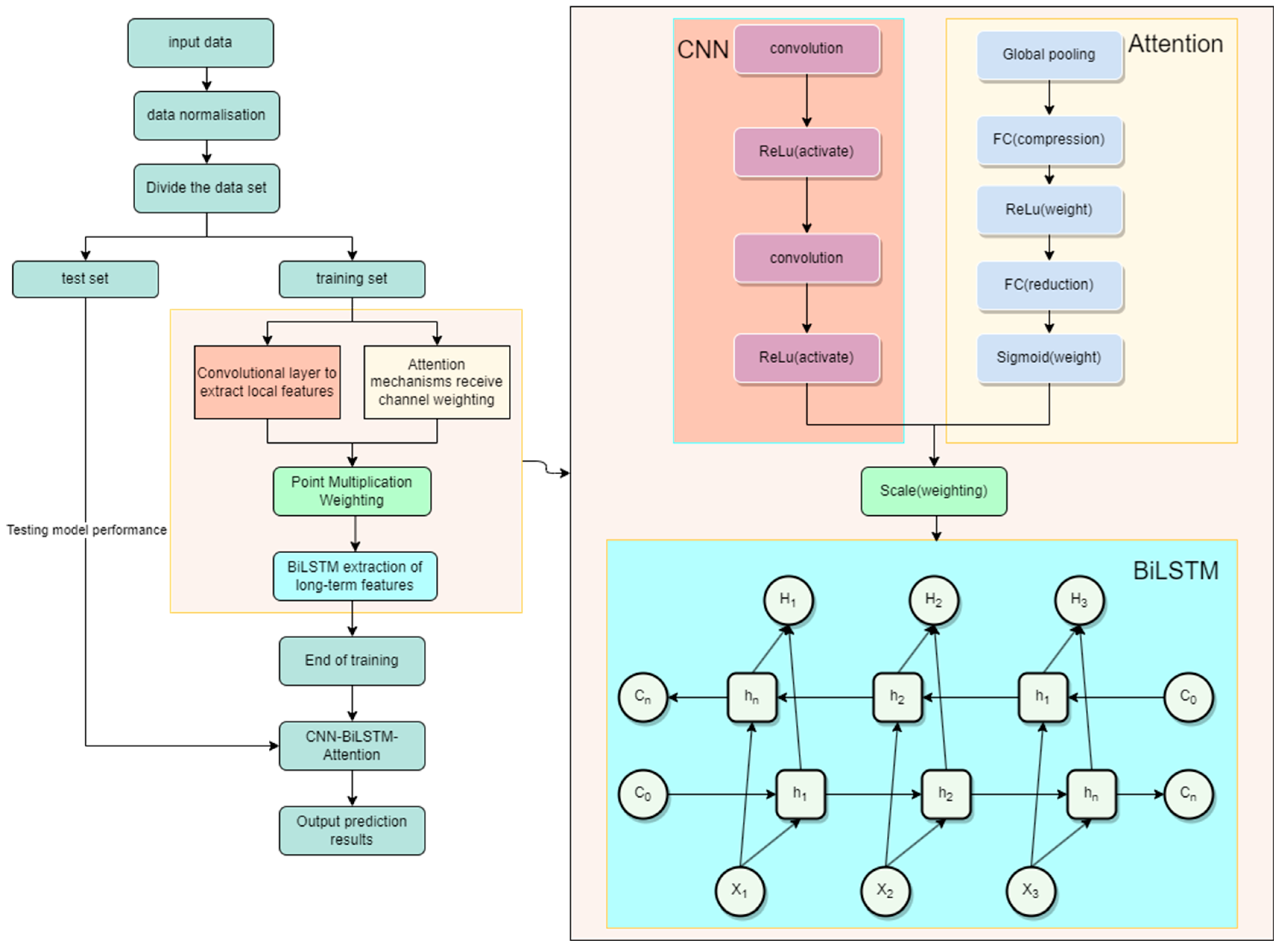
The prediction of inbound and outbound raw materials is an element of the temporal prediction problem, and the inbound and outbound dataset has prominent temporal characteristics due to the long period of the dataset, so it is important to select an appropriate model. The model is not a simple combination but combines the CNN and attention module into a parallel module, weights the local features extracted by the CNN through attention, and then inputs them into the BiLSTM to extract the long-term features so that the features can be thoroughly extracted and the phenomenon of the missing features of a neural network can be greatly reduced. Therefore, we used a hybrid CNN-BiLSTM-attention prediction model for inbound and outbound prediction, in which the CNN module in the model can extract the relatively complex spatial information features from the long sequence data with the local features of the data; BiLSTM can capture the long-term macroscopic dependency relationship of the temporal dataset through the forward and reverse information processing to capture long-term macroscopic dependencies in time series datasets; and the SE attention mechanism weights the dataset channels, boosting the channels that are useful for the target task and squeezing the channels that are of little use. The combination can complement the shortcomings and achieve better prediction.
2.2. Convolutional Neural Network
Convolutional neural networks (CNNs) are also widely used in time-series prediction [28], and Figure 1 shows their structure. The network consists of an input layer, a convolutional layer, a pooling layer, a fully connected layer, and an output layer. Each layer has its role, wherein the convolutional layer can extract features from the input data. The pooling layer performs a dimensionality reduction operation on the data to compress the features extracted by the convolutional layer, and the fully connected layer can weigh the compressed features. However, since the model and input data limit the size of the convolution kernel, the convolutional neural network cannot successfully extract features from long time-series data. It is more suitable for extracting local features, decreasing prediction accuracy [29] and leading many scholars to believe that traditional convolutional neural networks are incapable of time-series prediction tasks. However, recent research shows that convolutional neural networks can achieve good results through specific combination structures.
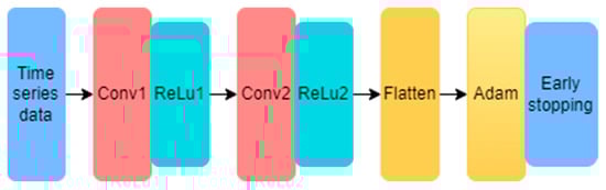
Figure 1.
Convolutional neural network timing processing steps.
2.3. Bidirectional Long Short-Term Memory Network
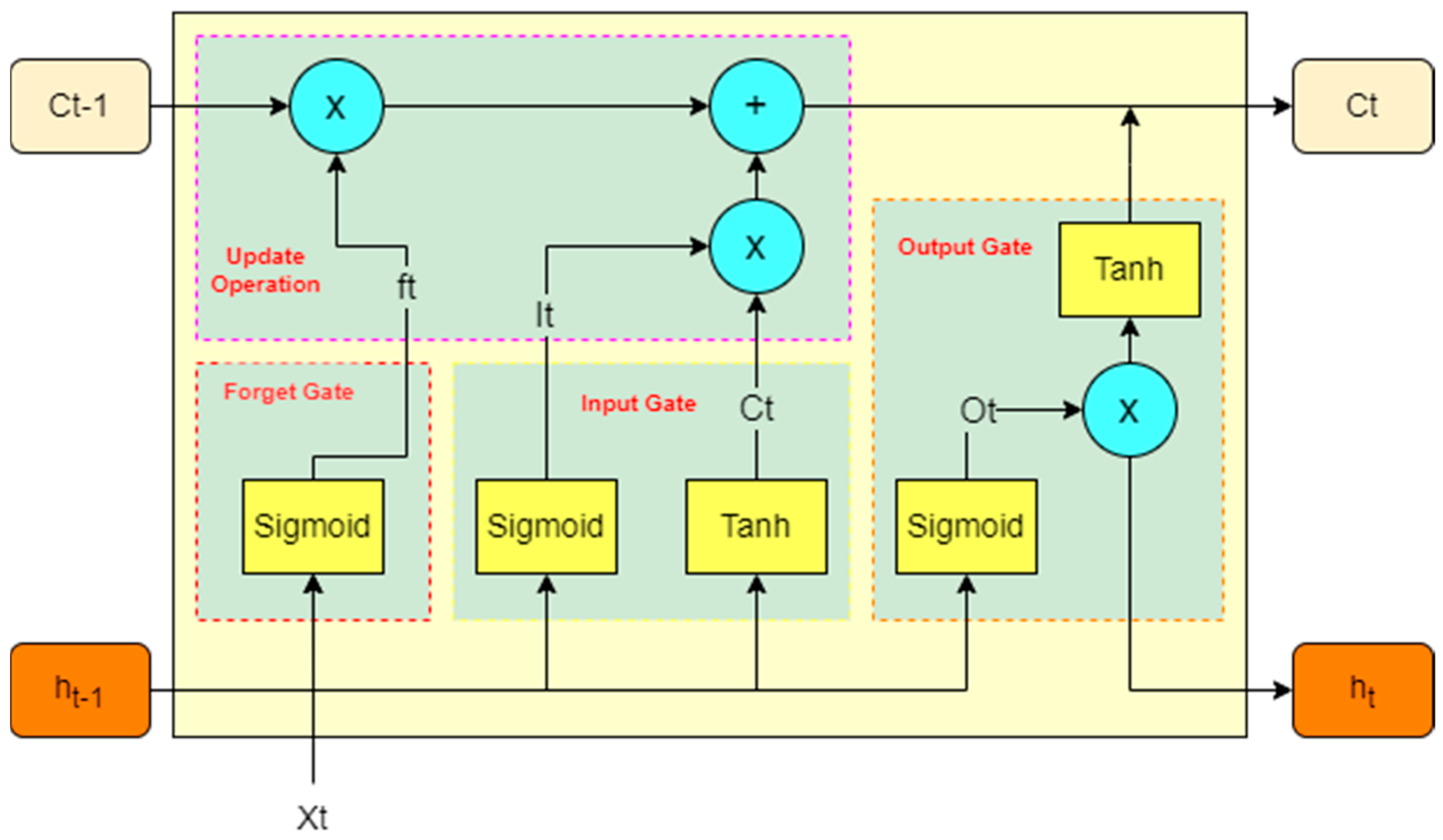
Due to the gradient problem with RNN [30], long short-term memory networks (LSTMs) can address the long-term dependency of temporal data [31,32]. Figure 2 shows the operational structure of the LSTM, which is divided into three gates, namely, the oblivion gate, input gate, and output gate, to control the state and to add the operation of updating the old information. The oblivion gate looks at ht-1 and Xt through a sigmoid unit to output a 0–1 vector (discard is 0, keep is 1). The input gate needs to decide on the updated information and obtain the new information through tanh. Next is the update operation of the LSTM. This operation will use the old information Ct-1, discard part of the information through the forgetting gate, and then add the candidate information through the inputs to become the new information Ct. The output gate will obtain the judgment condition through the sigmoid function and then through the tanh function to obtain the [−1, 1] vector, and then multiply the two together to obtain the output of the LSTM.
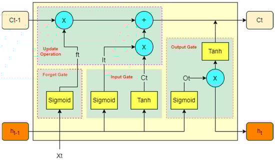
Figure 2.
LSTM operation structure diagram.
However, LSTM only has forward propagation, and the information processing is not thorough enough, so scholars proposed a bidirectional long short-term memory neural network. Adding another LSTM layer on top of the LSTM to achieve reverse information processing minimizes the shortcomings of a single LSTM and achieves a bidirectional reading of information.
2.4. Attention Mechanism
Attention mechanisms have achieved good results in machine-learning areas such as classification, prediction, and detection [33]. There are four stages of attention mechanisms: the spatial attention mechanism [34], the channel attention mechanism [35], the hybrid attention stage [36], and the self-attention mechanism [37].
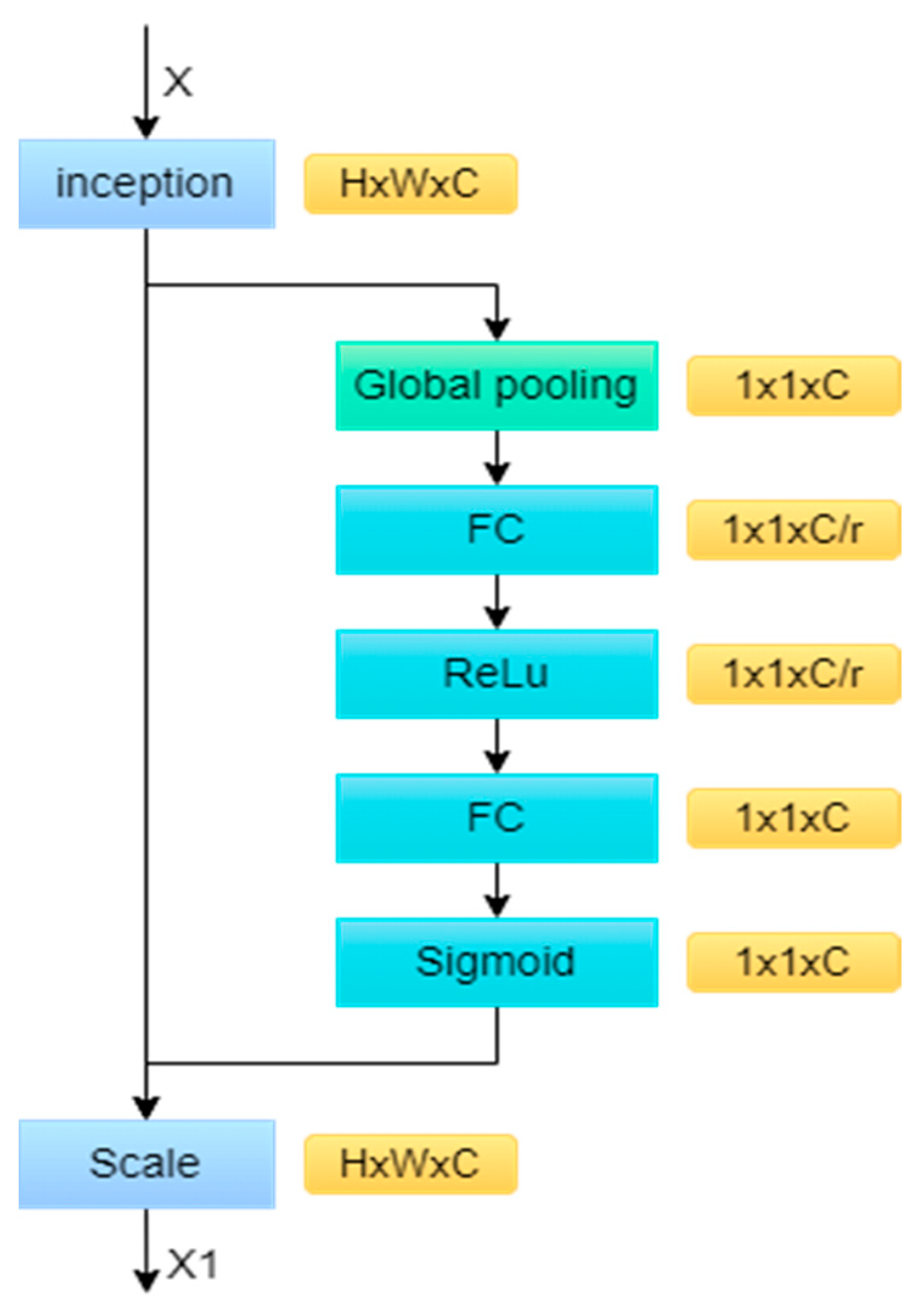
The SE attention mechanism can deal with the time-series features that the existing models ignore and extract the salient features from them. Figure 3 shows its structure; firstly, in the Squeeze operation, the data are compressed into feature vectors after global average pooling. Next is the Excitation operation. Firstly, the full connection layer compresses the channels and reduces the amount of computation. Then, through the RELU nonlinear activation layer, the channel size is restored by the fully connected layer. The Sigmoid function activates the weight of the channel. The Scale carries out the final weighting operation for each channel.

Figure 3.
Structure of the SE attention mechanism.
2.5. Model Prediction Steps
The prediction steps of the improved CNN-BiLSTM-attention model are shown in Figure 4. Firstly, the time-series data are inputted; secondly, the input data are normalized, then the training and test sets used for the experiments are divided, the training set is inputted into the network for training, the local features of the data are extracted using the convolutional layer and the activation function, and at the same time, the data are compressed into the feature vector by average pooling. Then, the weights of the feature vector are obtained by the fully connected layer and the activation function obtains the weight value of the feature vector. The features extracted from the convolutional layer are weighted by the dot product method and then enter the BiLSTM layer to extract the long-term temporal features of the data, which can constitute a complete trained CNN-BiLSTM-attention model. Subsequently, the test set is imported to test the accuracy of the model, and the evaluation indices are outputted to verify the prediction accuracy of the model.
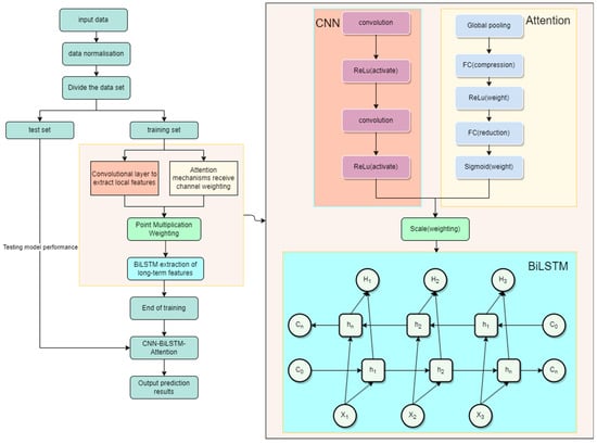
Figure 4.
Prediction steps of the model.
3. Experimental Setup and Evaluation of Results
The code program for this experiment is composed based on MATLAB writing. At the same time, in order to fully reflect the superiority of the CNN-BiLSTM-attention model improved using the attention mechanism adopted in this paper, this paper establishes five other comparison models: CNN, LSTM, CNN-LSTM, CNN-BiLSTM, CNN-LSTM-attention models.
In our study, to verify whether the best feature set is selected for training deep-learning models, we employ a cross-validation technique. By dividing the dataset into multiple subsets, in each cross-validation round, we use one of the subsets as the validation set and the remaining subsets as the training set. Repeating this process yields multiple sets of performance evaluation metrics that help assess the performance of the model with different feature sets. The best feature set is selected, thus improving the performance and generalization of the deep-learning model.
3.1. Data Collation
3.1.1. Data Collection
Data have a profound effect on the training of the model, and on the final result in re-timing prediction, different datasets are used, where data bias has a great impact on the accuracy of the deep-learning model [6].
The data in this paper come from large-scale manufacturing enterprises; the enterprises’ silica powder warehouses have daily information on the movement of silica powder in and out of the warehouse. Therefore, the database is constantly updated, and the inbound and outbound data in this paper are extracted from the database for the latest period of time. The data in this paper from the enterprise warehouse weighbridge system, successfully obtained from 1 November 2020 to 6 November 2023 , provide information on a total of 1101 days of silicon powder warehouse data. The silicon powder delivery container is a ton bag, the weight of each bag is 1 ton, and the capacity of each vehicle used by the manufacturer to deliver the bags is 32 bags. Therefore, the net weight of each car of silicon powder is about 32 tons, varying by not more than 0.2 tons. In order to facilitate the calculation, the default net weight of each car is 32 tons, and the unit of collation of the data used for the study is the number of vehicles. Table 1 shows some of the data in the dataset.

Table 1.
Silicon powder part of the inbound data.
Outbound data from the enterprise inventory system’s outbound ledger were successfully collected from 1 November 2021 to 31 October 2023, producing a total of 730 days of silicon powder outbound data. Because the weight of the outbound raw materials was primarily recorded in tons, in order to maintain consistency with the unit of the incoming data, the daily outbound tonnage was divided by 32. The units of the dataset were consistent with the incoming data using the number of cars. Some of the data are shown in Table 2.
Table 2.
Silicon powder part of the outbound data.
3.1.2. Exception Data Handling
Because the features of big data, in some cases, all appear to be cluttered, which can have many negative impacts on model training [38], there is a need to preprocess the data to improve the accuracy of the predictive model and obtain better results in the training of neural networks [39,40].
The first step in these improvements is the processing of data anomaly information. These types of data can occur for many reasons, such as sensor failure, artificial reasons, and abnormal events [41]. In this paper’s dataset, holiday factors were the leading cause of anomalies in the information in the dataset; for example, in the Spring Festival period, OEMs were rested, so there were 4–5 days of the incoming data being zero.
Scholars usually have three ways to deal with anomalous information. The first is the truncation method, which is to change the data that are greater than the threshold to the maximum threshold and the data that are smaller than the threshold to the minimum threshold; the second is to use special variables instead, such as the median, the maximum, the minimum, the average, and others; and the last is to use the missing value instead. Since the dataset in this paper does not have thresholds set and there are no missing data, the average value of the month are selected to replace these anomalies.
3.1.3. Data Normalization
Normalization adjusts or scales the dataset to a consistent reference line as a way of removing the effects of external factors on the data. For dynamic databases, a new normalization index has been proposed to assess the quality of the data and a unified PostgreSQL database has been constructed, which is able to provide users with an efficient data extraction tool [42]. Due to the complexity of the network structure in deep learning, internal variable bias or cannibalization of small data can easily occur during continuous iterative training. In addition, different evaluation indicators often have different quantitative outlines and units of quantification, which will affect the results of the data analysis. Our study must normalize the data to eliminate the influence of quantitative outlines between indicators. The normalized raw data, with the same order of magnitude for each indicator, are suitable for comprehensive comparative evaluation. Thus, normalization is required to optimize the convergence of the data.
The normalization method adopted in this paper is min–max normalization, which is a very flexible normalization method, and experiments by some scholars have proved that the average accuracy of the final output results of the decision tree model with min-max normalization applied can reach up to 99% in the task of machine learning [43].
Here, X2 is the normalized data of X1, Min(X) is the minimum data in the dataset, and Min(X) is the maximum data in the dataset.
3.1.4. Data Enhancement
The quantity and quality of the dataset have a significant impact on the output accuracy of deep learning. Too little quantity may appear as an overfitting phenomenon, and poor data quality may lead to model generalization and accuracy reduction [44]. In this paper, the inbound data have a total of 1101 pieces of data, and the outbound data have 730 pieces of data. This amount of data is still a relatively small sample size for the data scale of the convolutional neural network; therefore, to improve the model’s generalization ability and the robustness of the model, and to avoid overfitting problems, this work expands the sample data size by extracting the duplicate data from the dataset to generate random noise. Then, we linearly inserted the data into the dataset to augment the data.
If we use the inbound data as an example, with 1101 days of incoming data as a case study to analyze the trends and characteristics of the dataset, reasonable noise was added to the data so that the dataset was expanded to 7707 items, expanding the dataset by seven times. Figure 5 shows the scatter plot before and after the data enhancement: after adding reasonable noise to the dataset, the trend did not demonstrate a significant change, and the added noise permitted us to automatically identify the unreasonable data in the original dataset and construct a dataset with better generalization ability, thus improving the prediction accuracy of the model.
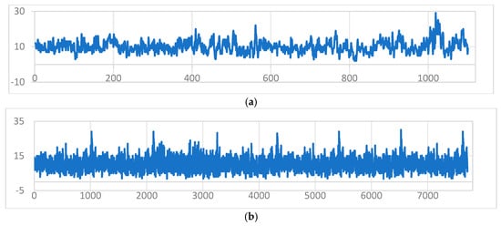
Figure 5.
Trends before and after data enhancement. (a) Trend chart before data enhancement; and (b) trend chart after data enhancement.
Due to the data enhancement process, the dataset in this paper already satisfies the requirements of the deep-learning model. In this paper, we divided the training set and the test set of the incoming data according to the ratio of 8:2; the share of the training set was 80 percent, and the share of the test set was 20 percent. Meanwhile, the ratio of training and test sets for dividing the outbound dataset was 7:3.
3.2. Model Evaluation
The selection of model evaluation metrics is a very important matter, and some scholars [6] have now delved into the application of various evaluation metrics in deep learning, highlighting the performance of different models in terms of the accuracy and assessment methods.
To ensure that the experimental output is more comprehensive and valid, we must assess the accuracy of the model, as well as the error. Therefore, to assess the performance of the prediction model, this study selected parameters such as the mean absolute error (MAE), mean square error (MSE), root mean square error (RMSE), mean absolute percentage error (MAPE), R-square (R2), and the model computation time.
3.2.1. Mean Absolute Error
Mean absolute error (MAE): When the MAE is 0, the model works optimally, and the larger the MAE, the worse the model works.
Here, is the model output’s predicted value and is the dataset’s actual value.
3.2.2. Mean Square Error
Mean square error (MSE): As with the MAE, the larger the value of the MSE, the worse the model is, and the best model has an MSE of zero. However, there is a square in the MSE, and it is possible to change its magnitude.
Here, is the model output’s predicted value and is the dataset’s actual value.
3.2.3. Root Mean Square Error
Root mean square error (RMSE): It is to open the root sign for the MSE. After opening the root sign, the result will be one level with the dataset, which can solve the shortcomings of the MSE to change the scale.
Here, is the model output’s predicted value and is the dataset’s actual value.
3.2.4. Mean Absolute Percentage Error
Mean absolute percentage error (MAPE): The MAPE has one more denominator than the MAE. When the MAPE is 0%, it indicates that the model is more effective; when the MAPE is higher t than 100%, it is less effective.
Here, is the model output’s predicted value and is the dataset’s actual value.
3.2.5. R-Square (R2)
R-square (R2): Commonly used to assess the goodness of fit of a model, i.e., whether the predicted array can achieve the fluctuating trend of the original array or the percentage it achieves, R2 can also be used to compare the performance between different model outputs.
Here, is the model output’s predicted value and is the dataset’s actual value.
3.2.6. Model Computation Time
The model computation time is one of the most intuitive indicators of the efficiency of model operation, and this experiment will use the average time of 50 model runs in seconds as the value of the model computation time.
3.2.7. I/O Uncertainty
Evaluating the I/O uncertainty in deep-learning models refers to evaluating the degree of uncertainty in the model’s processing of the input data and output results. This uncertainty may be caused by factors such as the noise in the input data, complexity of the model structure, and uncertainty in data preprocessing. For input uncertainty, the study is implemented by analyzing the change in the data distribution, by introducing data perturbation and changing the data distribution to assess the robustness and uncertainty of the model with respect to data changes. For output uncertainty, it is implemented by using the method of uncertainty estimation, by using Monte Carlo dropout to assess the uncertainty of the model output.
3.2.8. Sensitivity Analysis
Yeung D S et al. [45] suggest that the main purpose of the study of model sensitivity analysis is to allocate the uncertainty of the model output to the uncertainty of each input variable, and it can identify the features that have the most significant impact on the model’s prediction results, so that model optimization can be carried out to improve the prediction accuracy. The methods of model sensitivity analysis are mainly divided into two kinds. One kind is qualitative analysis, such as the scatterplot method; Bouayad D et al. [46] found that the scatterplot method can visualize the effect of individual inputs on outputs but cannot show the importance of each input data, so the applicability is greatly reduced [47]. The second is quantitative analysis, which has local and global aspects. LSA has great limitations when there is a nonlinear relationship between the input and output variables or a correlation between the input variables [45]. Therefore, scholars have proposed global sensitivity analysis (GSA) to solve this problem, and it has been successfully applied in many fields. For example, Asheghi R et al. [48] developed two artificial neural networks to predict riverbed loads, applied four sensitivity analysis methods, CAM, EM, RC and PaD, identified the most effective influences and ineffective factors for transporting sediment loads, and optimized the artificial neural network model to improve the prediction accuracy. Due to the instability of individual neural networks, it is not sufficient to be used as a sensitivity analysis parameter. Cao M S et al. [49], in order to solve this problem, proposed a parametric sensitivity analysis paradigm based on the integration of neural networks, which reduces the uncertainty of neural network modeling. The study then used variance-based global sensitivity analysis, which obtains the variance information through the perturbation of the input data or the predicted output of different batches, and then uses dropout variational inference to assess the degree of influence of each input feature or parameter on the output variance. Finally, the model’s response to input changes is understood based on the analysis results.
3.3. Model Parameter Setting
Parameter setting involves issues such as hyperparameter optimization, such as the number of hidden units, regularization interval, and learning rate selection. In this study, the prediction accuracy is used as an index, and the optimal hyperparameters are selected by comparing the different performances among the commonly used hyperparameters of deep-learning algorithms.
3.3.1. BiLSTM Hidden Cells
In BiLSTM, the number of hidden units is significant for the final prediction effect of the model. In this study, with other conditions unchanged, using R2 as the index, by comparing the final prediction results of the BiLSTM model with 2, 4, and 6 hidden units, respectively, as shown in Table 3, it is finally found that 6 hidden units can offer the best prediction effect.
Table 3.
Output comparison of the number of hidden units.
3.3.2. Normalized Interval
The experiment used the min–max method to normalize the data, as shown in Table 4. When comparing the difference between the two normalization ranges of [0, 1] and [−1, 1] through the inbound and outbound data, unsurprisingly, the sample output in the [−1, 1] range is much better, and therefore, the normalization ranges of the outbound, as well as the inbound, are delineated in the interval of [−1, 1].
Table 4.
Normalized interval output comparison.
3.3.3. Learning Rate
The learning rate directly determines the step size of the parameter update. If the learning rate is too large, it is difficult to converge to the predicted optimal value; on the contrary, if the learning rate is too small, the speed is too slow, which constitutes a waste of time [50]. Table 5 shows that with the R-square as an index, four different learning rates are constantly compared: 0.01, 0.001, 0.0001, and 0.0005. Finally, the learning rate was determined to be 0.0005.
Table 5.
Initial learning rate output comparison.
3.3.4. Optimization Algorithm Selection
Dying RELU is a difficult problem often encountered in the training of neural network models [51], where the output of the ReLU activation function may be consistently negative or close to zero during training, leading to neuron deactivation and resulting in the problem of vanishing gradients. This can lead to difficulties training the network or even failure to learn effective features. To solve this problem, there are usually four solutions: switching to other activation functions, adjusting the initialization strategy, adjusting the learning rate, and using the corresponding optimization algorithm. Among them, the use of corresponding optimization algorithms is the most intuitive and effective; practical optimization algorithms can help the model converge to the optimal solution faster and prevent the gradient from disappearing or exploding, and they can adjust the learning rate to improve the model’s generalization ability and performance. As shown in Table 6, three different optimization algorithms, such as Stochastic Gradient Descent (SGD), Adam, and Adagrad, were selected for comparison by observing the convergence of the loss function during the training process of outbound and inbound prediction and by comparing the accuracy of the three algorithms in terms of the final prediction. Finally, the Adam algorithm was chosen.
Table 6.
Optimization algorithm output comparison.
3.3.5. Overall Parameter Setting
Since the outbound and inbound datasets are of the same type and the overall trends are similar, the parameter settings for the outbound and inbound models are consistent. Table 7 shows the overall parameter settings for the six models.
Table 7.
Parameter setting for the inbound and outbound models.
3.4. Comparison of Inbound and Outbound Model Forecasts
This part mainly compares the prediction accuracy and error of the six models of access to the warehouse. To ensure the rigor of the experiment, the metrics were obtained from the average of 50 runs of the model. The prediction accuracy uses the R2 as the evaluation index; the prediction error uses the MAE, MSE, RMSE, MAPE, and model calculation time as the evaluation indices. Finally, the advantages and disadvantages of the models are analyzed by comparing the results.
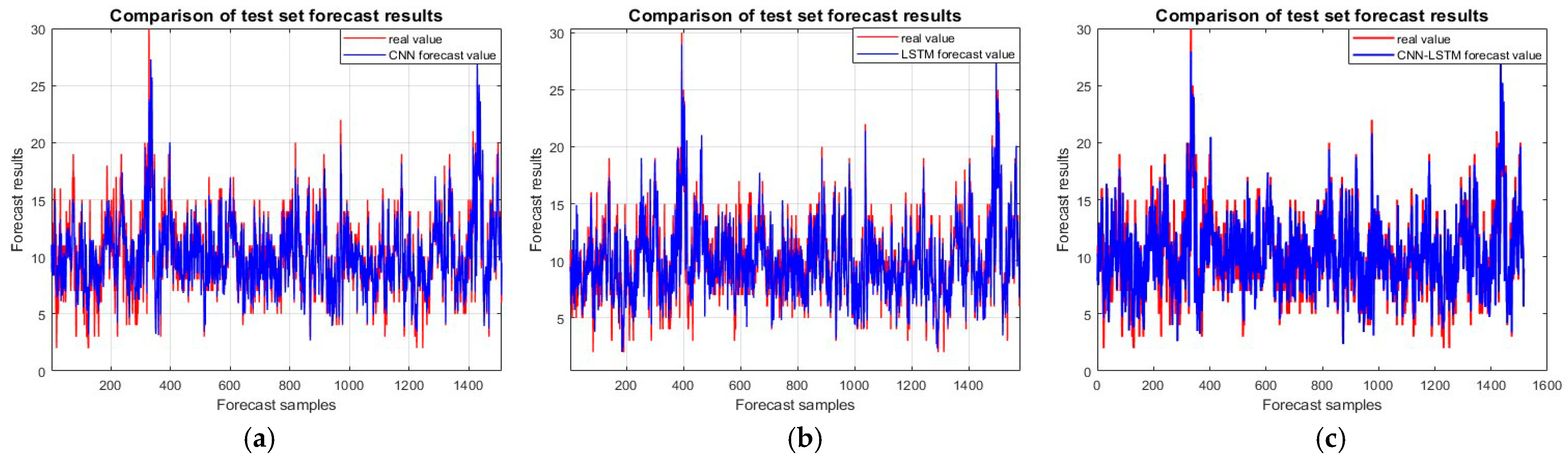
3.4.1. Comparison of Inbound Forecast Accuracy
In the test set comparison, as shown in Figure 6, the coefficient of determination R2 of the improved CNN-BiLSTM-attention prediction model reaches 0.92413, which demonstrates an improvement in the prediction accuracy of 6.338% compared to the CNN model and an improvement in the prediction accuracy by 4.09% compared to the LSTM model. Meanwhile, compared to the CNN-LSTM and CNN-BiLSTM models, the prediction accuracy is improved by 4.606% and 4.863%, respectively. The prediction accuracy of the CNN-LSTM-attention model is also weighted by the attention mechanism, but the prediction accuracy of the CNN-BiLSTM-attention model is still 4.533% higher than that of the CNN-LSTM-BiLSTM model.
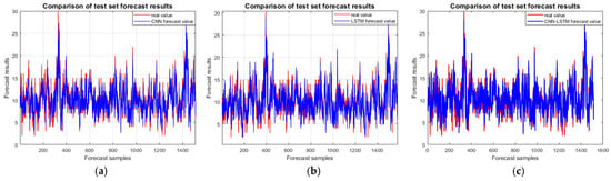
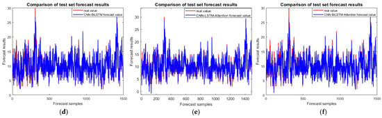
Figure 6.
Incoming model test set comparison chart: (a) CNN; (b) LSTM; (c) CNN-LSTM; (d) CNN-BiLSTM; (e) CNN-LSTM-attention; and (f) CNN-BiLSTM-attention.
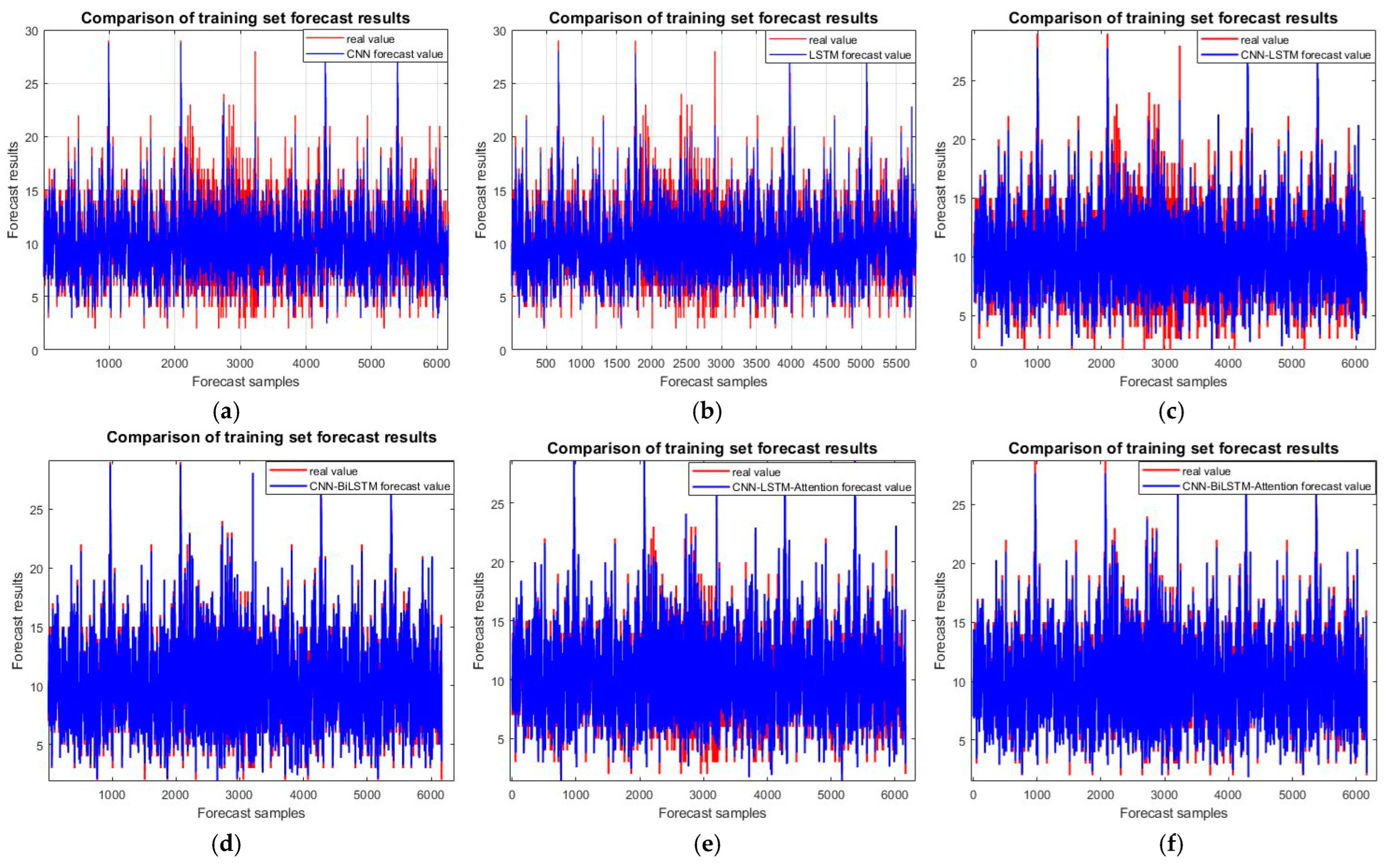
Figure 7 shows the comparison of the six models in the training set. The CNN-BiLSTM-attention model achieves a prediction accuracy of 0.96763, which is 9.48%, 6.837%, 4.995%, 1.396%, and 4.045% higher than those of the CNN, LSTM, CNN-LSTM, CNN-BiLSTM, and CNN-LSTM-attention models, respectively.
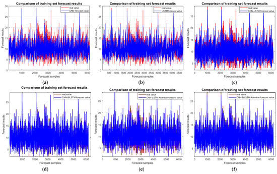
Figure 7.
Incoming model training set comparison chart: (a) CNN; (b) LSTM; (c) CNN-LSTM; (d) CNN-BiLSTM; (e) CNN-LSTM-attention; and (f) CNN-BiLSTM-attention.
3.4.2. Comparison of Inbound Forecast Error
Table 8 shows the error evaluation metrics for the six models. Due to differences in model operating environments, the evaluation indices of the six models were also obtained from the mean values after 50 runs to ensure the experimental results’ validity.
Table 8.
Indicators for the evaluation of the incoming forecasting models.
The first one is the mean absolute error (MAE) of the model, which is 41.79%, 30.44%, 26.53%, 16.43%, and 26.66% lower for the CNN-BiLSTM-attention model than for the five prediction models: CNN, LSTM, CNN-LSTM, CNN-BiLSTM, and CNN-LSTM-attention, respectively. In terms of the mean square error (MSE), the CNN-BiLSTM-attention model is also lower than the other five models, where the mean square error of CNN is 1.8107 times higher than that of the CNN-BiLSTM-attention model. The mean square error of the CNN-BiLSTM-attention model is also lower than that of the four models by 42.789%, 58.313%, 61.86%, and 57.58%, respectively. However, the magnitude of the MSE may change, so a further correction for the root mean square error (RMSE) is also required. As the table shows, for the root mean square error, the CNN-BiLSTM-attention model’s error is also much lower than for the remaining five models. For the mean absolute percentage error (MAPE), the errors of all six models are very close to each other, but the CNN-BiLSTM-attention model still has the lowest error. Finally, the running efficiency of the models—because of the varying complexity of the models—is, in descending order, as follows: LSTM > CNN > CNN-LSTM > CNN-BiLSTM-attention > CNN-LSTM-attention > CNN-BiLSTM.
3.4.3. Comparison of Outbound Forecast Accuracy
The comparison of the outbound model accuracy is similar to the inbound comparison; both are unfolded from the training set and the test set, and the accuracy index of the model is the R2. A larger R2 indicates that the model prediction accuracy is higher and, vice versa, a smaller R2 indicates that the model prediction accuracy is lower. Again, from both the prediction set and the training set, the prediction results are still the average of the results obtained from 50 runs of the model.
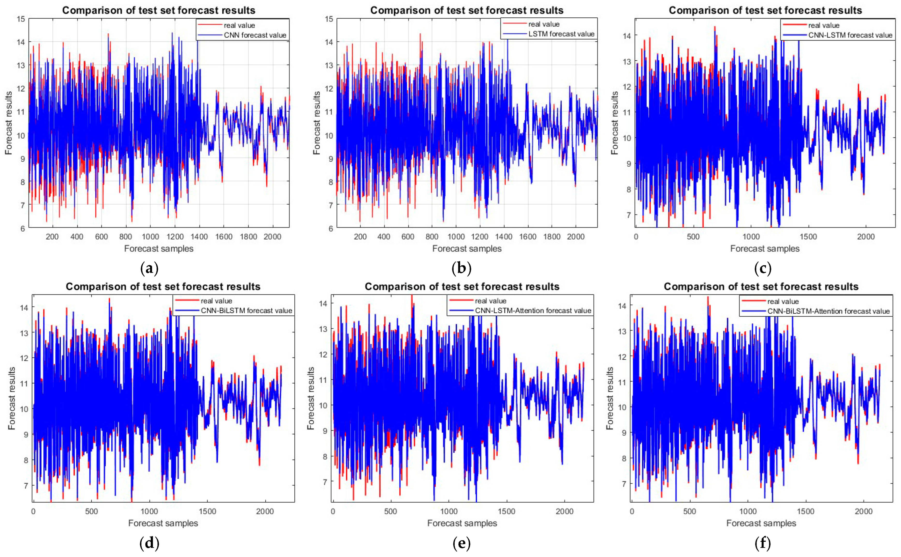
The prediction accuracy of the test set is a direct reflection of the model’s prediction accuracy and is crucial for comparing the final results. Figure 8 shows a comparison of the accuracy of the test set for the six models. The CNN-BiLSTM-attention prediction model has the highest accuracy, with an R-square value as high as 0.98618, which is 3.088%, 6.038%, 0.882%, 1.854%, and 3.363% higher than those for the five prediction models of CNN, LSTM, CNN-LSTM, CNN-BiLSTM, and CNN-LSTM-attention, respectively.
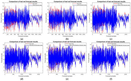
Figure 8.
Outcoming model test set comparison chart: (a) CNN; (b) LSTM; (c) CNN-LSTM; (d) CNN-BiLSTM; (e) CNN-LSTM-attention; and (f) CNN-BiLSTM-attention.
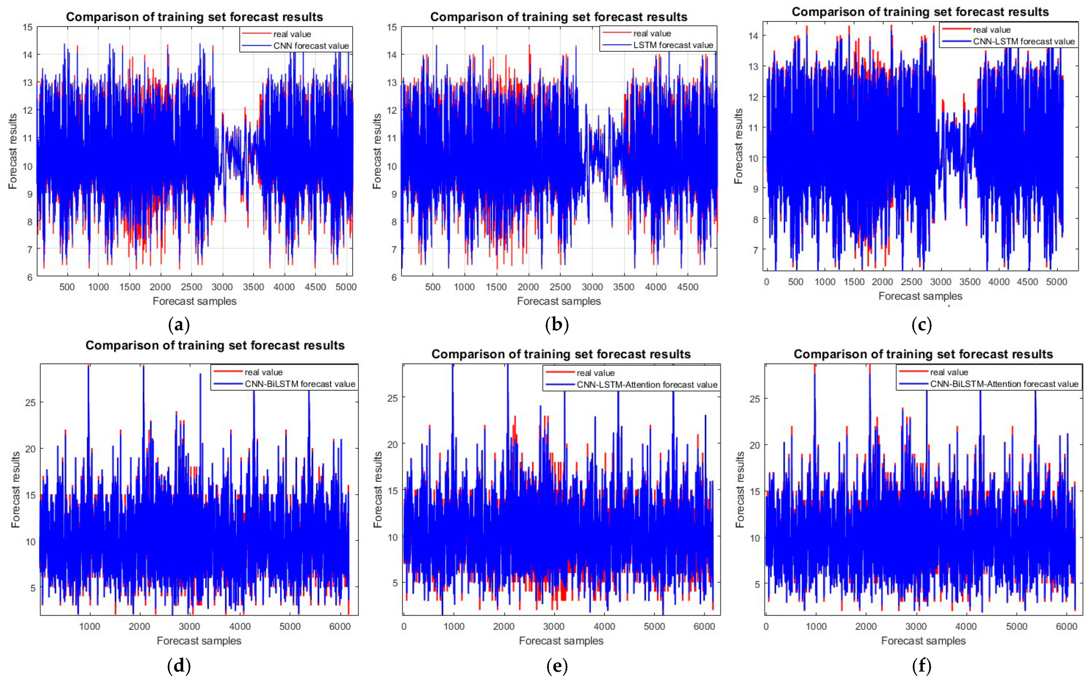
Figure 9 shows the output of the six models on the training set, where the accuracy of all six models is close. However, the CNN-BiLSTM-attention model has the highest accuracy, which is 1.606%, 3.279%, 0.413%, 0.641%, and 1.498%, higher than the prediction accuracies of the other five models, respectively.
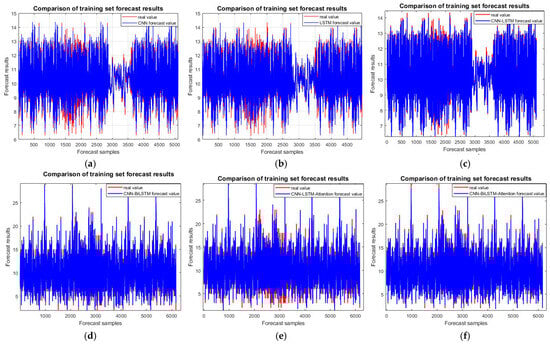
Figure 9.
Outcoming model training set comparison chart: (a) CNN; (b) LSTM; (c) CNN-LSTM; (d) CNN-BiLSTM; (e) CNN-LSTM-attention; and (f) CNN-BiLSTM-attention.
3.4.4. Comparison of Outbound Forecast Error
Table 9 shows the error metrics for the six outbound forecasting models and considers the different environments in which the models are run. For experimental rigor, the evaluation metrics are taken from the mean values obtained after 50 runs of the models.
Table 9.
Indicators for evaluating the outbound forecasting model.
As can be seen from the comparison of the data in the table, the CNN-BiLSTM-attention model is still the best among the three models in all indicators except the computation time. In comparing the mean absolute error (MAE), the CNN-BiLSTM-attention model has the lowest error with an MAE of 0.12022. In contrast, the LSTM model has the highest mean absolute error, which is 2.1 times higher than that of the CNN-BiLSTM-attention model. Moreover, the CNN-BiLSTM-attention model, in comparison to the four other models of CNN, CNN-LSTM, CNN-BiLSTM, and CNN-LSTM-attention, has an MAE that is 73.68%, 26.99%, 7.61%, and 71.98% lower, respectively. For the mean square error, MSE, the CNN-BiLSTM-attention model also has the lowest error, and the CNN model and the LSTM model have the highest errors, 3.233 times and 5.407 times that of the CNN-BiLSTM-attention model. In the root mean square error (RMSE) comparison, the error of the LSTM model is 2.337 times higher than that of the CNN-BiLSTM-attention model, and the error of the CNN-BiLSTM-attention model is 80.88%, 28.17%, 52.19%, and 72.4% lower than those of the other four models, respectively. In terms of the mean absolute percentage error, MAPE, all six models are very close to each other, and the CNN-BiLSTM-attention model has an error of 0.01206, which is still the lowest among the six models. Regarding the average computation time of the models, the order of efficiency of the six models, from high to low, is as follows: LSTM > CNN > CNN-LSTM > CNN-BiLSTM-attention > CNN-LSTM-attention > CNN-BiLSTM.
3.5. Analysis of Experimental Results
From the above evaluation metrics, it can be concluded that the improved CNN-BiLSTM-attention model used in this study has the highest prediction accuracy and the lowest prediction error among the six models for outbound and inbound predictions. Firstly, due to the relatively simple structure of the CNN and LSTM models, the prediction accuracies of these two models are lower than those of the other four models, and the average computation time is also the lowest; the CNN-BiLSTM model is lower than the CNN-LSTM model in each error of the temporal data processing due to the use of the bi-directional long- and short-term memory neural network. The improved CNN-BiLSTM-attention model has the highest prediction accuracy and the lowest prediction error among the six models. The CNN-BiLSTM-attention model adds the attention mechanism, which can deal with some temporal features missed by the network and can weigh the channels, which enables the model to focus on critical temporal features; therefore, it has a more powerful temporal data-processing ability than the CNN-BiLSTM model. It can guarantee prediction accuracy with the minimum error, and it has high generalizability at the same time. CNN-LSTM-attention has a more significant overall error and a low prediction accuracy because it does not process the time-series data in both directions and due to the incomplete long-term feature extraction.
From the perspective of the model computational efficiency, the CNN and LSTM models have the lowest computational time. However, they have the highest computational error and the lowest accuracy. The CNN-LSTM model, due to its relatively simple structure, has the second-highest computational time after the CNN and LSTM models. However, the accuracy of the inbound and outbound predictions is lower than that of the CNN-BiLSTM-attention model by 4.533% and 3.363%, respectively. The CNN-BiLSTM and CNN-LSTM-attention models are lower than the CNN-BiLSTM-attention model in model prediction accuracy and computational efficiency. As the enterprise’s inbound and outbound statistics are recorded in days, the timeliness requirement of the prediction is low. The difference in the extremes in the average computation time between the outbound and inbound of the above six models is 445.19 s and 256.2 s, respectively, which is relatively low for a one-day statistical unit. However, because silicon powder is costly and has considerable volatility, the enterprise must accurately control the quantity of silicon powder moving in and out of the warehouse, and the enterprise needs to consider the inventory costs, production needs, material prices, and other factors. Hence, the prediction accuracy of the silicon powder moving in and out of the warehouse is rigorous, and the timeliness requirement is low. The prediction efficiency of the CNN-BiLSTM-attention model is good. The prediction accuracy for outgoing and incoming inventory is ahead of the other five models. Therefore, combining the experimental data with the enterprise requirements, the CNN-BiLSTM-attention model is the best model among these six models used for inbound and outbound prediction.
4. Conclusions
This study fully demonstrates the effectiveness of the CNN-BiLSTM-attention model in predicting the movement of silica powder in and out of a warehouse. Predicting the raw material in/out data with relative accuracy is crucial for enterprises to achieve inventory control, optimize inventory structure, and reduce costs. However, in enterprise inventory prediction, it is difficult to grasp the characteristics of the raw material data and predict the lack of information technology, resulting in poor prediction accuracy. Addressing the difficulty of forecasting access to the warehouse, this study used silicon powder, an essential raw material for new energy enterprises, as an example and used an improved CNN-BiLSTM-attention hybrid model to predict the movement of silicon powder in and out of the warehouse. The model extracts local features from the time-series data through the CNN, then uses the attention mechanism to weight the feature channels, and finally, extracts long-term time-series features from the data through BiLSTM.
This study compared the improved CNN-BiLSTM-attention hybrid model used in this paper with five other models with the same model parameter settings. It uses machine-learning evaluation indices, such as the R2, MAE, MSE, RMSE, and MAPE, to evaluate the model’s accuracy and error. The comprehensive experimental results show that the improved CNN-BiLSTM-attention model had the highest accuracy, generalization, and practicability in both inbound and outbound prediction, and the model can effectively and accurately predict the inbound and outbound movement of silica powder, which can help enterprises to enhance their inventory control.
Although the dataset in this study came from the access information of one company, it can still be applied to other fields. The access data of materials that need to be predicted in this field can be collected, and the data can be organized by means of data enhancement and normalization. Through the tuning of parameters and hyperparameters to achieve optimization effects on different datasets, the adaptability of the model can be increased, and the prediction accuracy of the model using different datasets can be improved.
However, there are some limitations in this study, which are affected by some objective factors, such as weather and sudden disasters, which also affect the accuracy of the final inventory prediction. Meanwhile, as the market fluctuates and the operating conditions of enterprises are different, the model also needs to be continuously updated to meet the needs and requirements of the enterprise for inventory control, which will require continuous research in the future. This can be achieved by optimizing the model structure, e.g., by upgrading the attention mechanism or combining models using TCN networks. At the same time, for different enterprises and different raw materials, the model parameters and hyperparameters can be adjusted according to the model operation, and the model normalization intervals can be adjusted to make the model more suitable for the new dataset and to improve the model prediction accuracy.
Author Contributions
Conceptualization, D.G. and P.D.; methodology, D.G. and P.D.; software, P.D.; formal analysis, P.D.; investigation, P.D. and Y.S.; resources, P.D., X.Z. and Z.Y.; data curation, P.D.; writing—original draft preparation, D.G. and P.D.; writing—review and editing, D.G. and P.D.; supervision, D.G. All authors have read and agreed to the published version of the manuscript.
Funding
This study was supported by the Key Research and Development Program Project of the Department of Science and Technology of the Autonomous Region (grant no. 2022B01015) and the Science and Technology Program Project of the Bureau of Ecology, Environment and Industrial Development of Ganquanbao Economic and Technological Development Zone (Industrial Zone) (grant.no. GKJ2023XTWL04).
Data Availability Statement
The original contributions presented in the study are included in the article, further inquiries can be directed to the corresponding author/s.
Conflicts of Interest
Author Xiaojiang Zhang was employed by Xinjiang Xinte Energy Logistics Co. and author Zhen Yang was employed by Xinjiang Hualing Logistics & Distribution Co. The remaining authors declare that the research was conducted in the absence of any commercial or financial relationships that could be construed as a potential conflict of interest.
References
- Wong, J.M.; Chan, A.P.; Chiang, Y. Forecasting construction manpower demand: A vector error correction model. Build. Environ. 2007, 42, 3030–3041. [Google Scholar] [CrossRef]
- Wingerden, V.E.; Basten, R.; Dekker, R. More grip on inventory control through improved forecasting: A comparative study at three companies. Int. J. Prod. Econ. 2014, 157, 220–237. [Google Scholar] [CrossRef]
- Luo, X.M.; Li, J.B.; Hu, P. E-commerce inventory optimization strategy based on time series forecasting. Syst. Eng. 2014, 32, 91–98. [Google Scholar]
- Guo, X.; Liu, C.; Xu, W. A Prediction-Based Inventory Optimization Using Data Mining Models. In Proceedings of the Seventh International Joint Conference on Computational Sciences & Optimization, Beijing, China, 4–6 July 2014; IEEE Computer Society: Washington, DC, USA, 2014; pp. 611–615. [Google Scholar] [CrossRef]
- Zhou, H.; Ding, D.; Li, Y.; Wu, M. Research on inventory demand forecast based on BP neural network. Inf. Technol. 2016, 40, 38–41. [Google Scholar] [CrossRef]
- Liang, H.; Liu, S.; Du, J.; Hu, Q.; Yu, X. Review of Deep Learning Applied to Time Series Prediction. J. Front. Comput. Sci. Technol. 2023, 17, 1285–1300. [Google Scholar] [CrossRef]
- Gu, J.; Wang, Z.; Kuen, J.; Ma, L.; Shahroudy, A.; Shuai, B.; Liu, T.; Wang, X.; Wang, G.; Cai, J.; et al. Recent advances in convolutional neural networks. Pattern Recognit. 2018, 77, 354–377. [Google Scholar] [CrossRef]
- Tuo, S.; Chen, T.; He, H.; Feng, Z.; Zhu, Y.; Liu, F.; Li, C. A Regional Industrial Economic Forecasting Model Based on a Deep Convolutional Neural Network and Big Data. Sustainability 2021, 13, 12789. [Google Scholar] [CrossRef]
- Chen, Y.; Kang, Y.; Chen, Y.; Wang, Z. Probabilistic forecasting with temporal convolutional neural network. Neurocomputing 2020, 399, 491–501. [Google Scholar] [CrossRef]
- Lim, B.; Arık, S.; Loeff, N.; Pfister, T. Temporal Fusion Transformers for interpretable multi-horizon time series forecasting. Int. J. Forecast. 2021, 37, 1748–1764. [Google Scholar] [CrossRef]
- Zhang, P.; Yin, X.; Li, S.; Wang, X. The Short-term Forecasting of Power Load in Agricultural Greenhouses Based on VMD-CNN-LSTM. Inf. Control. 2024, 53, 238–249. [Google Scholar] [CrossRef]
- Yu, B.; Meng, W.; Yu, T.; Zhou, C.; Guo, F. Short-term load prediction of smart parks based on ICEEMDAN-CNN-K-shape. Foreign Electron. Meas. Technol. 2023, 42, 103–112. [Google Scholar] [CrossRef]
- Yuan, R.; Wei, H.; Fu, Z.J.; Li, J. Research on the commodity sales forecast of e-commerce enterprises integrating CNN and WDF model. Comput. Eng. Appl. 2024, 10, 1–10. [Google Scholar]
- Lu, J.; Wang, Y.; Zhu, Y.; Liu, J.; Xu, Y.; Yang, H.; Wang, Y. DACLnet: A Dual-Attention-Mechanism CNN-LSTM Network for the Accurate Prediction of Nonlinear InSAR Deformation. Remote Sens. 2024, 16, 2474. [Google Scholar] [CrossRef]
- Wei, Z.; Shaohua, J.; Gang, B.; Yang, C.; Chengyang, P.; Haixing, X. A Method for Sound Speed Profile Prediction Based on CNN-BiLSTM-Attention Network. J. Mar. Sci. Eng. 2024, 12, 414. [Google Scholar] [CrossRef]
- Ma, Z.; Sun, Y.; Ji, H.; Li, S.; Nie, S.; Yin, F. A CNN-BiLSTM-Attention approach for EHA degradation prediction based on time-series generative adversarial network. Mech. Syst. Signal Process. 2024, 215, 111443. [Google Scholar] [CrossRef]
- Taper, M.L.; Ponciano, J.M. Evidential statistics as a statistical modern synthesis to support 21st century science. Popul. Ecol. 2016, 58, 9–29. [Google Scholar] [CrossRef]
- Hernández, S.; López, J.L. Uncertainty quantification for plant disease detection using Bayesian deep learning. Appl. Soft Comput. 2020, 96, 106597. [Google Scholar] [CrossRef]
- Abbas, S.A.; Chunling, S.; Stefan, L. A Novel Approach to Uncertainty Quantification in Groundwater Table Modeling by Automated Predictive Deep Learning. Nat. Resour. Res. 2022, 31, 1351–1373. [Google Scholar] [CrossRef]
- Zhang, Y.M.; Wang, H. Multi-head attention-based probabilistic CNN-BiLSTM for day-ahead wind speed forecasting. Energy 2023, 278, 127865. [Google Scholar] [CrossRef]
- Tang, C.; Zhang, Y.; Wu, F.; Tang, C. An Improved CNN- BILSTM Model for Power Load Prediction in Uncertain Power Systems. Energies 2024, 17, 2312. [Google Scholar] [CrossRef]
- Hu, Z.; Deng, J.; Han, J.; Yuan, K. Review on application of graph neural network in traffic prediction. J. Traffic Transp. Eng. 2023, 23, 39–61. [Google Scholar] [CrossRef]
- Zhang, Z.; Qu, L.; Li, X.; Zhang, M.; Li, Z. Traffic flow prediction with missing data based on spatial-temporal convolutional neural networks. Comput. Eng. Appl. 2022, 58, 259–265. [Google Scholar] [CrossRef]
- Maya, R.C.; Carazas, G.F.; Barajas, H.F.; Rodriguez, P.C.; Manco, U.O. Remaining Useful Life Prediction of Lithium-Ion Battery Using ICC-CNN-LSTM Methodology. Energies 2023, 16, 7081. [Google Scholar] [CrossRef]
- Rashid, J.; Abdul NN, R.; Salah, B.; Ur, R.Z.; Salma, B. Mathematical analysis of the transmission dynamics of viral infection with effective control policies via fractional derivative. Nonlinear Eng. 2023, 12, 20220342. [Google Scholar] [CrossRef]
- Rashid, J.; Abdul NN, R.; Salah, B.; Ur, R.Z. Fractional insights into Zika virus transmission: Exploring preventive measures from a dynamical perspective. Nonlinear Eng. 2023, 12, 20220352. [Google Scholar] [CrossRef]
- Haiour, M.; Hocine, M.E.A.B.L.; Jan, R.; Himadan, A.; Boulaaras, S. Existence and uniqueness for the evolutionary impulse control problem using an asynchronous algorithms. Partial. Differ. Equ. Appl. Math. 2024, 11, 100766. [Google Scholar] [CrossRef]
- Li, B.; Liu, K.; Gu, J.; Jiang, W. Review of the researches on convolutional neural networks. Comput. Era 2021, 4, 8–12+17. [Google Scholar] [CrossRef]
- Kang, M.; Song, J.; Fan, P.; Gao, B.; Zhou, X.; Li, Z. Survey of network traffic forecast based on deep learning. Comput. Eng. Appl. 2021, 57, 1–9. [Google Scholar] [CrossRef]
- Pascanu, R.; Mikolov, T.; Bengio, Y. On the Difficulty of Training Recurrent Neural Networks. 2012. Available online: https://www.JMLR.org (accessed on 10 June 2024).
- Graves, A. Generating Sequences with Recurrent Neural Networks. arXiv 2013, arXiv:1308.0850. [Google Scholar]
- Liu, J.; Song, Z. Overview of recurrent neural networks. Control Decis. 2022, 37, 2753–2768. [Google Scholar] [CrossRef]
- Zhang, W. Semantic Analysis for Cross-Media Data. Master’s Thesis, Hangzhou Dianzi University, Hangzhou, China, 2019. [Google Scholar] [CrossRef]
- Mnih, V.; Heess, N.; Graves, A.; Kavukcuoglu, K. Recurrent Models of Visual Attention. arXiv 2014, arXiv:1406.6247. [Google Scholar]
- Jie, H.; Li, S.; Samuel, A.; Gang, S.; Enhua, W. Squeeze-and-Excitation Networks. IEEE Trans. Pattern Anal. Mach. Intell. 2019, 42, 2011–2023. [Google Scholar] [CrossRef]
- Deng, J.; Liu, J.; Ma, X.; Qin, X.; Jia, Z. Local Feature Enhancement for Nested Entity Recognition Using a Convolutional Block Attention Module. Appl. Sci. 2023, 13, 9200. [Google Scholar] [CrossRef]
- Yin, F.; Li, S.; Ji, M.; Wang, Y. Neural TV program recommendation with label and user dual attention. Appl. Intell. 2021, 52, 19–32. [Google Scholar] [CrossRef]
- Huang, C.; Huang, Y. Information fusion early warning of rail transit signal operation and maintenance based on big data of internet of things. Sustain. Comput. Inform. Syst. 2022, 35, 100763. [Google Scholar] [CrossRef]
- Xiao, Z.; Gang, W.; Yuan, J.; Chen, Z.; Li, J.; Wang, X.; Feng, X. Impacts of data preprocessing and selection on energy consumption prediction model of HVAC systems based on deep learning. Energy Build. 2022, 258, 111832. [Google Scholar] [CrossRef]
- Luo, S.; Ding, C.; Cheng, H.; Zhang, B.; Zhao, Y.; Liu, L. Estimated ultimate recovery prediction of fractured horizontal wells in tight oil reservoirs based on deep neural networks. Adv. Geo-Energy Res. 2022, 6, 111–122. [Google Scholar] [CrossRef]
- Wang, W. Analysis of database abnormally information mining method based on machine learning. Electron. Technol. 2022, 51, 24–25. [Google Scholar]
- Abbaszadeh Shahri, A.; Shan, C.; Larsson, S.; Johansson, F. Normalizing Large Scale Sensor-Based MWD Data: An Automated Method toward A Unified Database. Sensors 2024, 24, 1209. [Google Scholar] [CrossRef] [PubMed]
- Lanjewar, M.G.; Parate, R.K.; Parab, J.S. Machine learning approach with data normalization technique for early stage detection of hypothyroidism. In Artificial Intelligence Applications for Health Care; CRC Press: Boca Raton, FL, USA, 2022; pp. 91–108. [Google Scholar]
- Wang, J.M.; Chen, X.Y.; Yang, Z.Z.; Shi, C.Y.; Qian, Z.K. Impact of different data augmentation methods on model recognition accuracy. Comput. Eng. Appl. 2020, 56, 11–24. [Google Scholar]
- Yeung, D.S.; Cloete, I.; Shi, D.; Ng, W.W.Y. Sensitivity Analysis for Neural Networks; Springer: Berlin/Heidelberg, Germany, 2010. [Google Scholar] [CrossRef]
- Bouayad, D.; Emeriault, F. Modeling the relationship between ground surface settlements induced by shield tunneling and the operational and geological parameters based on the hybrid PCA/ANFIS method. Tunn. Undergr. Space Technol. Inc. Trenchless Technol. Res. 2017, 68, 142–152. [Google Scholar] [CrossRef]
- Sobol′, I.M. Global sensitivity indices for nonlinear mathematical models and their Monte Carlo estimates. Math. Comput. Simul. 2001, 55, 271–280. [Google Scholar] [CrossRef]
- Asheghi, R.; Hosseini, A.S.; Saneie, M.; Shahri, A.A. Updating the neural network sediment load models using different sensitivity analysis methods: A regional application. J. Hydroinform. 2020, 22, 562–577. [Google Scholar] [CrossRef]
- Cao, M.S.; Pan, L.X.; Gao, Y.F.; Novák, D.; Ding, Z.C.; Lehký, D.; Li, L.X. Neural network ensemble-based parameter sensitivity analysis in civil engineering systems. Neural Comput. Appl. 2017, 28, 1583–1590. [Google Scholar] [CrossRef]
- Wang, X. A Review of Research on Gradient Descent and Optimization Algorithms. Comput. Knowl. Technol. 2022, 18, 71–73. [Google Scholar] [CrossRef]
- Qipin, C.; Wenrui, H.; Juncai, H. A weight initialization based on the linear product structure for neural networks. Appl. Math. Comput. 2022, 415, 126722. [Google Scholar] [CrossRef]


Disclaimer/Publisher’s Note: The statements, opinions and data contained in all publications are solely those of the individual author(s) and contributor(s) and not of MDPI and/or the editor(s). MDPI and/or the editor(s) disclaim responsibility for any injury to people or property resulting from any ideas, methods, instructions or products referred to in the content. |
© 2024 by the authors. Licensee MDPI, Basel, Switzerland. This article is an open access article distributed under the terms and conditions of the Creative Commons Attribution (CC BY) license (https://creativecommons.org/licenses/by/4.0/).