
A Physics-Based Equivalent Circuit Model and State of Charge Estimation for Lithium-Ion Batteries
Abstract
:1. Introduction
2. Electrochemical Model of Lithium-Ion Battery
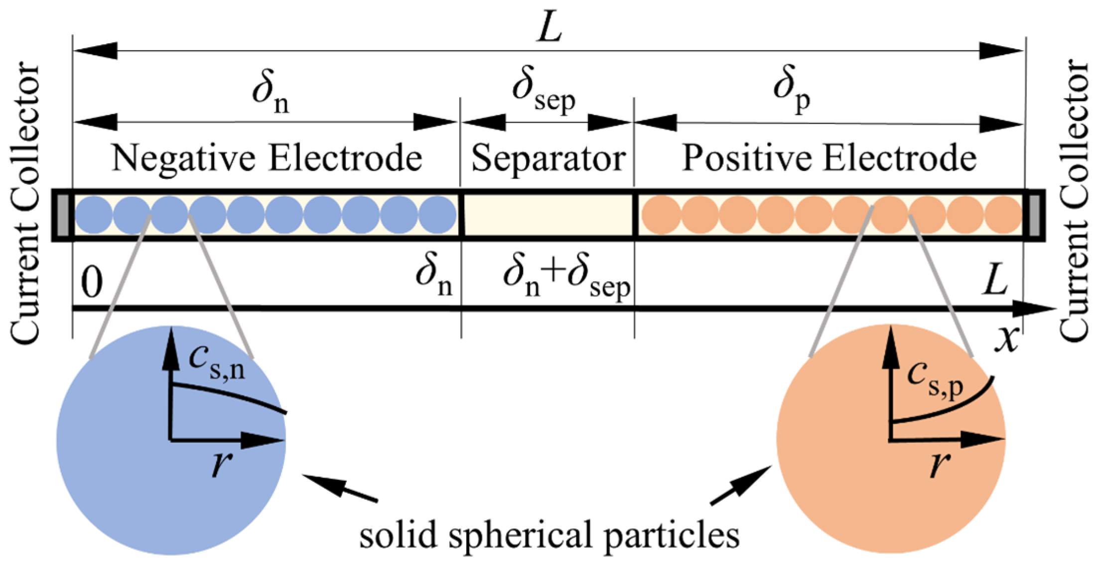
2.1. The Pseudo-Two-Dimensional Model
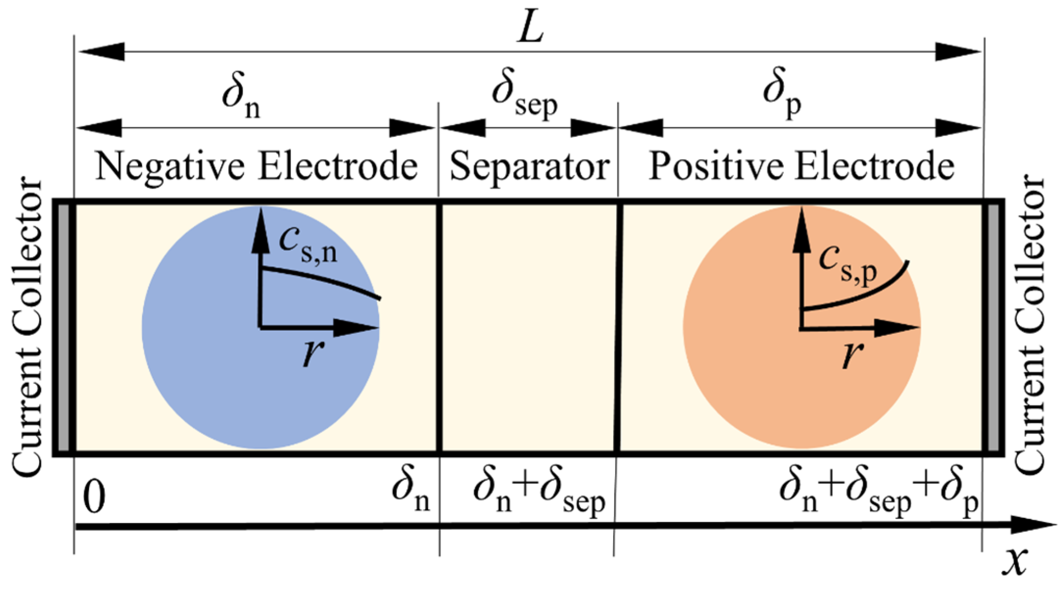
2.2. The Extended Single Particle Model
2.3. Improved Extended Single Particle Model
3. ECM of Improved Extended Single Particle Model
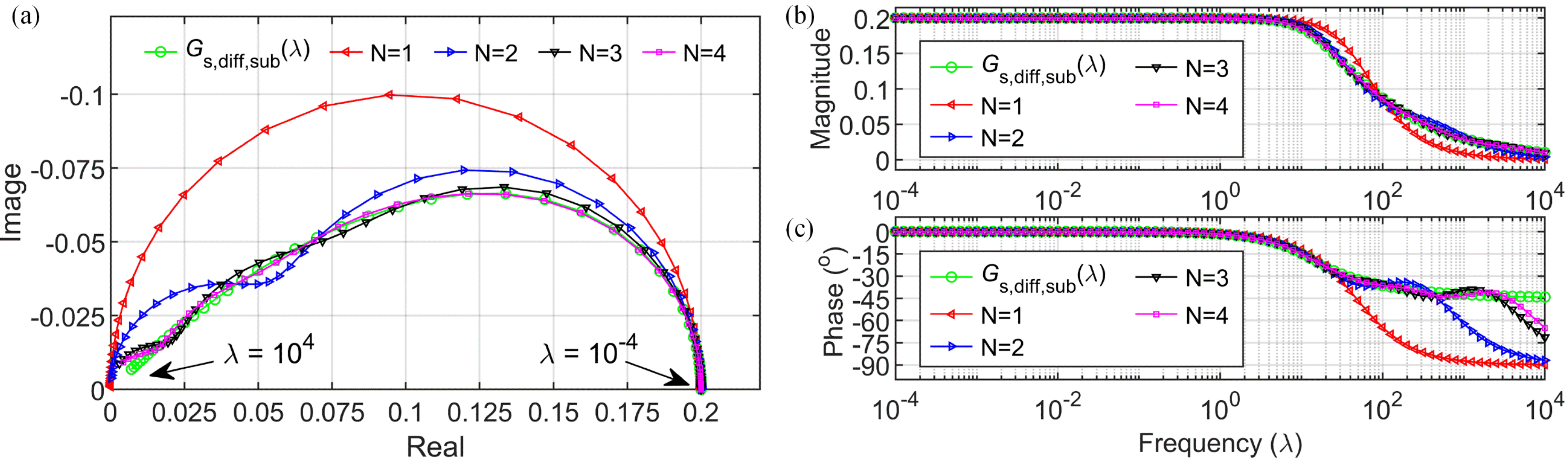
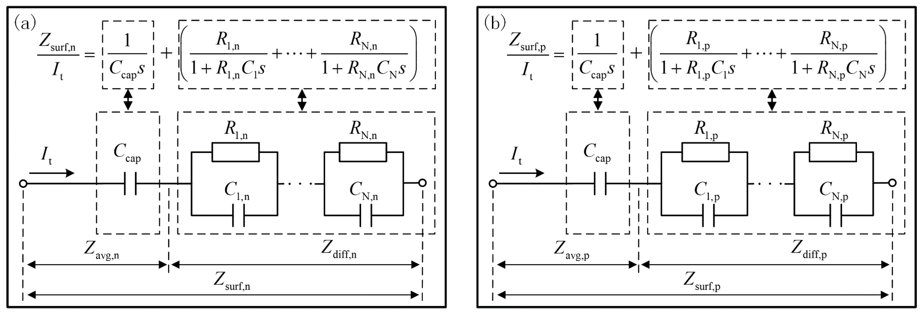
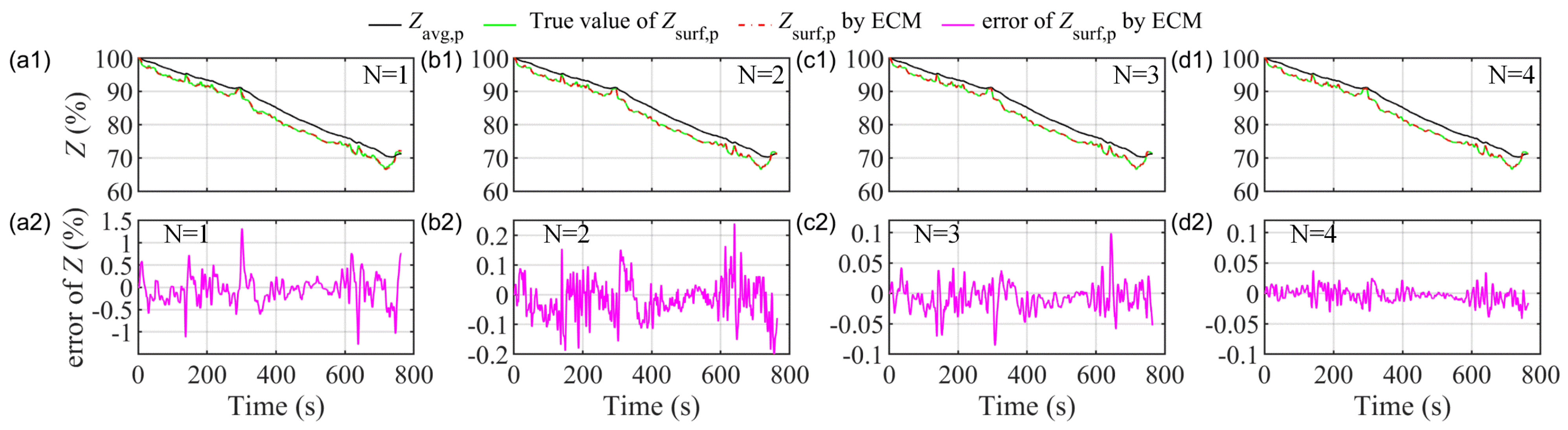
3.1. Solid Phase Diffusion Approximation
3.2. Electrolyte Diffusion Approximation
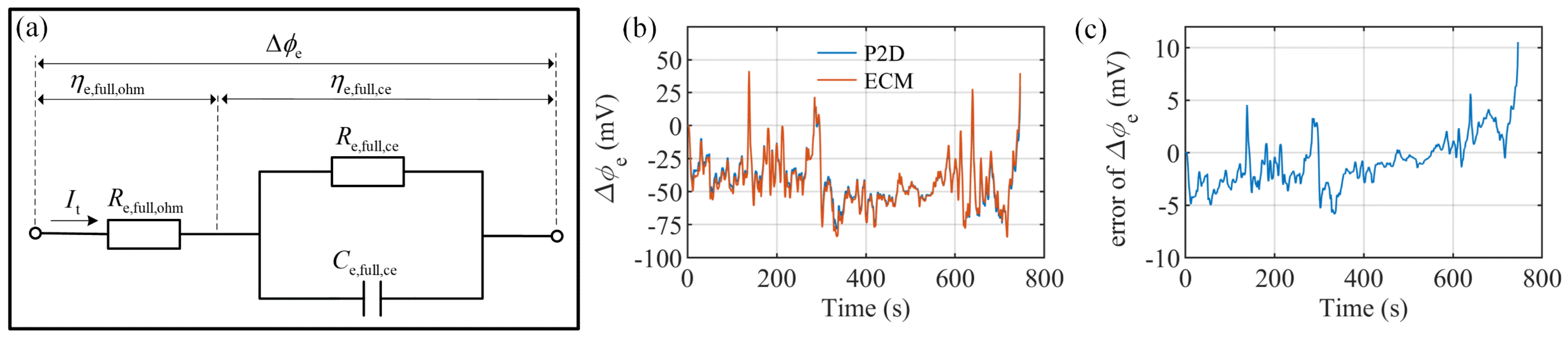
3.3. Electrolyte Potential Approximation
3.4. Approximation of Correction Terms in IESP
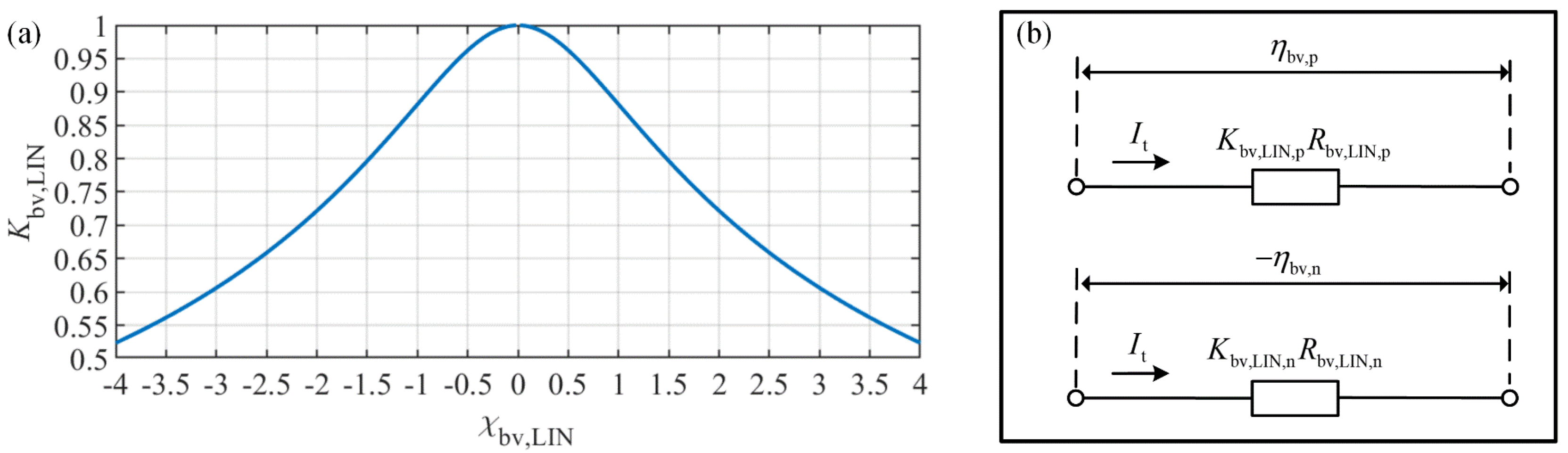
3.5. ECM of Electrochemical Reaction
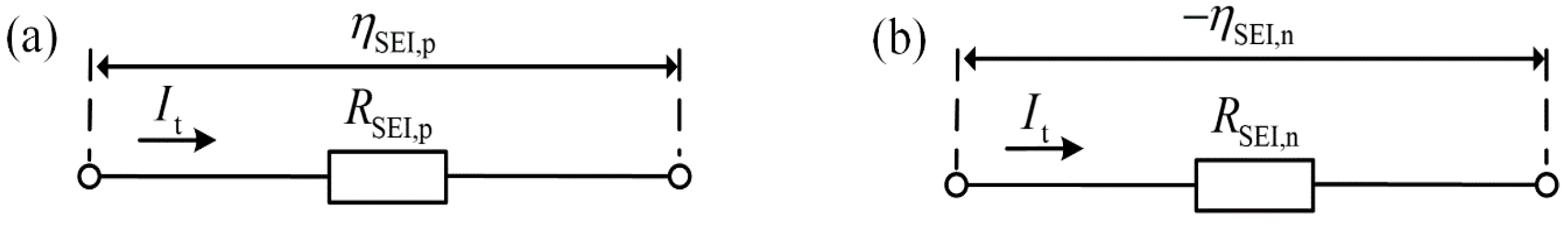
3.6. ECM of SEI Film Resistance
3.7. Construction of the Full ECM of IESP Model
4. Model Verification under Different Load Profiles
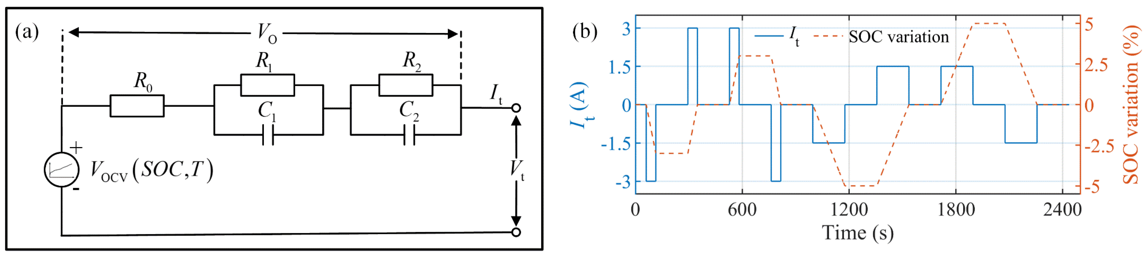
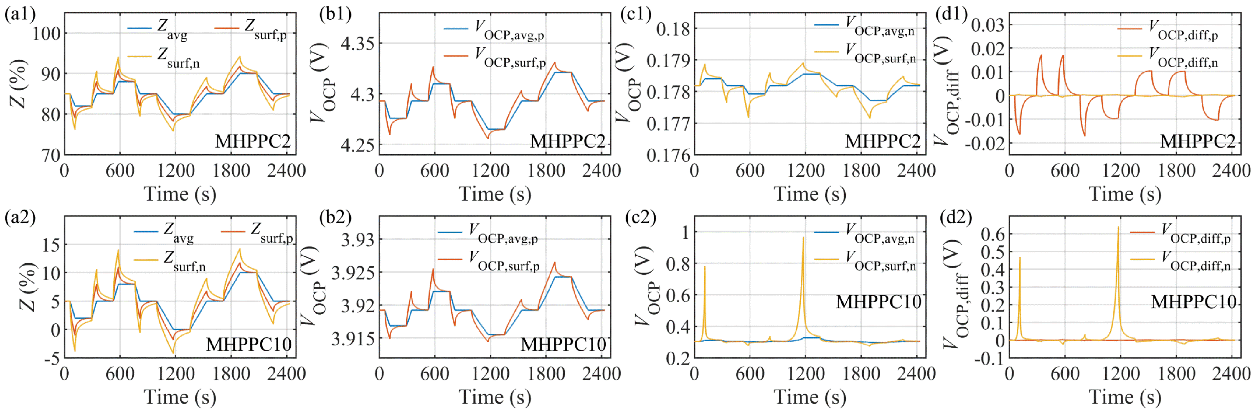
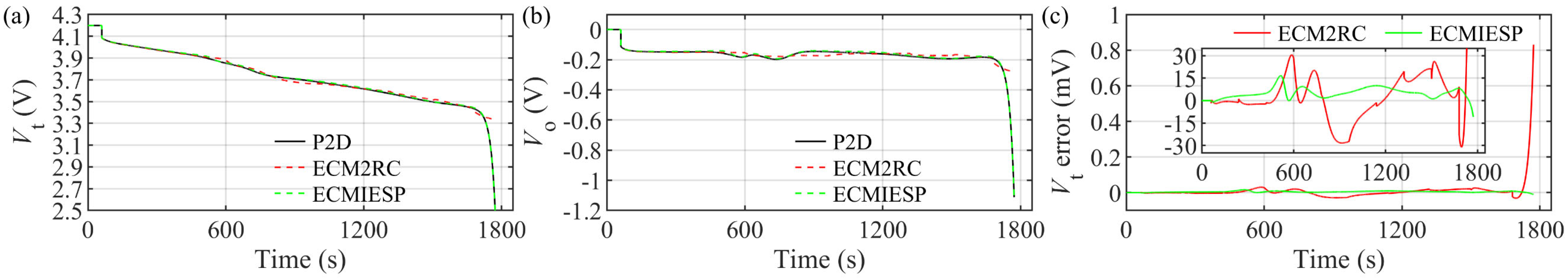
4.1. Model Verification under MHPPC Test and Parameter Identification of ECM2RC
4.2. Model Verification under HPPC Test
4.3. Model Verification under Constant Current Discharge Test
4.4. Model Verification under HWFET Test
5. SOC Estimation Based on the ECMIESP Model
5.1. SOC Estimation Based on the ECMIESP Model through Extended Kalman Filter
5.2. Results and Comparison
6. Conclusions
Author Contributions
Funding
Data Availability Statement
Conflicts of Interest
References
- Ramadesigan, V.; Northrop, P.W.C.; De, S.; Santhanagopalan, S.; Braatz, R.D.; Subramanian, V.R. Modeling and Simulation of Lithium-Ion Batteries from a Systems Engineering Perspective. J. Electrochem. Soc. 2012, 159, 31–45. [Google Scholar] [CrossRef]
- Christensen, G.; Younes, H.; Hong, H.; Widener, C.; Wu, J.J. Nanofluids as Media for High Capacity Anodes of Lithium-Ion Battery—A Review. J. Nanofluids 2019, 8, 657–670. [Google Scholar] [CrossRef]
- Li, X.; Fan, G.; Pan, K.; Wei, G.; Zhu, C.; Rizzoni, G.; Canova, M. A physics-based fractional order model and state of energy estimation for lithium ion batteries. Part I: Model development and observability analysis. J. Power Sources 2017, 367, 187–201. [Google Scholar] [CrossRef]
- He, H.; Xiong, R.; Fan, J. Evaluation of Lithium-Ion Battery Equivalent Circuit Models for State of Charge Estimation by an Experimental Approach. Energies 2011, 4, 582–598. [Google Scholar] [CrossRef]
- Li, J.; Klee Barillas, J.; Guenther, C.; Danzer, M.A. A comparative study of state of charge estimation algorithms for LiFePO4 batteries used in electric vehicles. J. Power Sources 2013, 230, 244–250. [Google Scholar] [CrossRef]
- Xiong, R.; Sun, F.; Gong, X.; Gao, C. A data-driven based adaptive state of charge estimator of lithium-ion polymer battery used in electric vehicles. Appl. Energy 2014, 113, 1421–1433. [Google Scholar] [CrossRef]
- Li, Y.; Chen, J.; Lan, F. Enhanced online model identification and state of charge estimation for lithium-ion battery under noise corrupted measurements by bias compensation recursive least squares. J. Power Sources 2020, 456, 227984. [Google Scholar] [CrossRef]
- Tekin, M.; Karamangil, M.İ. Comparative analysis of equivalent circuit battery models for electric vehicle battery management systems. J. Energy Storage 2024, 86, 111327. [Google Scholar] [CrossRef]
- Doyle, M.; Fuller, T.F.; Newman, J. Modeling of galvanostatic charge and discharge of the lithium/polymer/insertion cell. J. Electrochem. Soc. 1993, 140, 1526–1533. [Google Scholar] [CrossRef]
- Guo, M.; Sikha, G.; White, R.E. Single-Particle Model for a Lithium-Ion Cell: Thermal Behavior. J. Electrochem. Soc. 2011, 158, 122–132. [Google Scholar] [CrossRef]
- Prada, E.; Di Domenico, D.; Creff, Y.; Bernard, J.; Sauvant-Moynot, V.; Huet, F. Simplified Electrochemical and Thermal Model of LiFePO4-Graphite Li-Ion Batteries for Fast Charge Applications. J. Electrochem. Soc. 2012, 159, 1508–1519. [Google Scholar] [CrossRef]
- Luo, W.; Lyu, C.; Wang, L.; Zhang, L. A new extension of physics-based single particle model for higher charge–discharge rates. J. Power Sources 2013, 241, 295–310. [Google Scholar] [CrossRef]
- Ali, H.A.A.; Raijmakers, L.H.; Chayambuka, K.; Danilov, D.L.; Notten, P.H.; Eichel, R. A comparison between physics-based Li-ion battery models. Electrochim. Acta 2024, 493, 144360. [Google Scholar] [CrossRef]
- Kumar, R.R.; Bharatiraja, C.; Udhayakumar, K.; Devakirubakaran, S.; Sekar, S.; Mihet-Popa, L. Advances in batteries, battery modeling, battery management system, battery thermal management, SOC, SOH, and charge/discharge characteristics in EV applications. IEEE Access 2023, 12, 43984–43999. [Google Scholar] [CrossRef]
- Tameemi, A.Q.; Kanesan, J.; Khairuddin, A.S.M. Model-based impending lithium battery terminal voltage collapse detection via data-driven and machine learning approaches. J. Energy Storage 2024, 86, 111279. [Google Scholar] [CrossRef]
- Kurucan, M.; Özbaltan, M.; Yetgin, Z.; Alkaya, A. Applications of artificial neural network based battery management systems: A literature review. Renew. Sustain. Energy Rev. 2024, 192, 114262. [Google Scholar] [CrossRef]
- Renold, A.P.; Kathayat, N.S. Comprehensive review of machine learning, deep learning, and digital twin data-driven approaches in battery health prediction of electric vehicles. IEEE Access 2024, 12, 43984–43999. [Google Scholar] [CrossRef]
- Han, X.; Ouyang, M.; Lu, L.; Li, J. Simplification of physics-based electrochemical model for lithium ion battery on electric vehicle. Part I: Diffusion simplification and single particle model. J. Power Sources 2015, 278, 802–813. [Google Scholar] [CrossRef]
- Santhanagopalan, S.; Guo, Q.; Ramadass, P.; White, R.E. Review of models for predicting the cycling performance of lithium ion batteries. J. Power Sources 2006, 156, 620–628. [Google Scholar] [CrossRef]
- Khaleghi Rahimian, S.; Rayman, S.; White, R.E. Extension of physics-based single particle model for higher charge–discharge rates. J. Power Sources 2013, 224, 180–194. [Google Scholar] [CrossRef]
- Tanim, T.R.; Rahn, C.D.; Wang, C. State of charge estimation of a lithium ion cell based on a temperature dependent and electrolyte enhanced single particle model. Energy 2015, 80, 731–739. [Google Scholar] [CrossRef]
- Han, X.; Ouyang, M.; Lu, L.; Li, J. Simplification of physics-based electrochemical model for lithium ion battery on electric vehicle. Part II: Pseudo-two-dimensional model simplification and state of charge estimation. J. Power Sources 2015, 278, 814–825. [Google Scholar] [CrossRef]
- Marcicki, J.; Canova, M.; Conlisk, A.T.; Rizzoni, G. Design and parametrization analysis of a reduced-order electro-chemical model of graphite/LiFePO4 cells for SOC/SOH estimation. J. Power Sources 2013, 237, 310–324. [Google Scholar] [CrossRef]
- Xu, J.; Sun, C.; Ni, Y.; Lyu, C.; Wu, C.; Zhang, H.; Feng, F. Fast identification of micro-health parameters for retired batteries based on a simplified P2D model by using padé approximation. Batteries 2023, 9, 64. [Google Scholar] [CrossRef]
- Yuan, S.; Jiang, L.; Yin, C.; Wu, H.; Zhang, X. A transfer function type of simplified electrochemical model with modified boundary conditions and Padé approximation for Li-ion battery: Part 1. lithium concentration estimation. J. Power Sources 2017, 352, 245–257. [Google Scholar] [CrossRef]
- Yuan, S.; Jiang, L.; Yin, C.; Wu, H.; Zhang, X. A transfer function type of simplified electrochemical model with modified boundary conditions and Padé approximation for Li-ion battery: Part 2. Modeling and parameter estimation. J. Power Sources 2017, 352, 258–271. [Google Scholar] [CrossRef]
- Li, X.; Pan, K.; Fan, G.; Lu, R.; Zhu, C.; Rizzoni, G.; Canova, M. A physics-based fractional order model and state of energy estimation for lithium ion batteries. Part II: Parameter identification and state of energy estimation for LiFePO4 battery. J. Power Sources 2017, 367, 202–213. [Google Scholar] [CrossRef]
- Guo, D.; Yang, G.; Feng, X.; Han, X.; Lu, L.; Ouyang, M. Physics-based fractional-order model with simplified solid phase diffusion of lithium-ion battery. J. Energy Storage 2020, 30, 101404. [Google Scholar] [CrossRef]
- Ouyang, M.; Liu, G.; Lu, L.; Li, J.; Han, X. Enhancing the estimation accuracy in low state-of-charge area: A novel onboard battery model through surface state of charge determination. J. Power Sources 2014, 270, 221–237. [Google Scholar] [CrossRef]
- Andre, D.; Meiler, M.; Steiner, K.; Walz, H.; Soczka-Guth, T.; Sauer, D.U. Characterization of high-power lithium-ion batteries by electrochemical impedance spectroscopy. II: Modelling. J. Power Sources 2011, 196, 5349–5356. [Google Scholar] [CrossRef]
- Fleischer, C.; Waag, W.; Heyn, H.; Sauer, D.U. On-line adaptive battery impedance parameter and state estimation considering physical principles in reduced order equivalent circuit battery models Part 1. Requirements, critical review of methods and modeling. J. Power Sources 2014, 260, 276–291. [Google Scholar] [CrossRef]
- Fleischer, C.; Waag, W.; Heyn, H.; Sauer, D.U. On-line adaptive battery impedance parameter and state estimation considering physical principles in reduced order equivalent circuit battery models: Part 2. Parameter and state estimation. J. Power Sources 2014, 262, 457–482. [Google Scholar] [CrossRef]
- Zheng, Y.; Gao, W.; Han, X.; Ouyang, M.; Lu, L.; Guo, D. An accurate parameters extraction method for a novel on-board battery model considering electrochemical properties. J. Energy Storage 2019, 24, 100745. [Google Scholar] [CrossRef]
- Dao, T.; Vyasarayani, C.P.; McPhee, J. Simplification and order reduction of lithium-ion battery model based on porous-electrode theory. J. Power Sources 2012, 198, 329–337. [Google Scholar] [CrossRef]
- Subramanian, V.R.; Diwakar, V.D.; Tapriyal, D. Efficient Macro-Micro Scale Coupled Modeling of Batteries. J. Electrochem. Soc. 2005, 152, 2002–2008. [Google Scholar] [CrossRef]
- Rahn, C.D.; Wang, C. Battery Systems Engineering, 1st ed.; John Wiley & Sons: West Sussex, UK, 2013; pp. 27–28. [Google Scholar]
- Zhang, R.; Li, X.; Sun, C.; Yang, S.; Tian, Y.; Tian, J. State of charge and temperature joint estimation based on ultrasonic reflection waves for lithium-ion battery applications. Batteries 2023, 9, 335. [Google Scholar] [CrossRef]
- Xiong, R.; Cao, J.; Yu, Q.; He, H.; Sun, F. Critical Review on the Battery State of Charge Estimation Methods for Electric Vehicles. IEEE Access 2018, 6, 1832–1843. [Google Scholar] [CrossRef]
- Plett, G.L. Extended Kalman filtering for battery management systems of LiPB-based HEV battery packs Part 3. State and parameter estimation. J. Power Sources 2004, 134, 277–292. [Google Scholar] [CrossRef]


| Governing Equations | Boundary Conditions | ||
|---|---|---|---|
| Negative electrode electrolyte phase diffusion: | (1) | ||
| Negative electrode electrolyte phase potential: | (2) | ||
| Negative electrode Solid phase potential: | (3) | ||
| Negative electrode solid phase diffusion: | (4) | ||
| Separator area electrolyte phase diffusion: | (5) | ||
| Separator area electrolyte phase potential: | (6) | ||
| Positive electrode electrolyte phase diffusion: | (7) | ||
| Positive electrode electrolyte phase potential: | (8) | ||
| Positive electrode Solid phase potential: | (9) | ||
| Positive electrode solid phase diffusion: | (10) | ||
| Butler–Volmer equation: | (11) | ||
| Solid/Electrolyte interface (SEI) Ohmic effect: | (12) | ||
| Surface potential of the active particle: | (13) | ||
| Electrode potential balance: | (14) | ||
| Terminal voltage: | (15) |
| Parameters | Symbol | Unit | Negative Electrode | Separator | Positive Electrode |
|---|---|---|---|---|---|
| Faraday’s constant | 96487 | ||||
| Gas constant | 8.314 | ||||
| Temperature | 298 | ||||
| Bruggman exponent | 1.5 | ||||
| Electrode plate area | 0.05 | 0.05 | 0.05 | ||
| Electrolyte volume fraction | 0.3 | 1 | 0.3 | ||
| Region thickness | |||||
| Initial electrolyte concentration | 1000 | 1000 | 1000 | ||
| Li ion transference number | 0.4 | 0.4 | 0.4 | ||
| activity coefficient | 0 | 0 | 0 | ||
| Particle radius | |||||
| Filler volume fraction | 0.1 | 0.2 | |||
| Active material volume fraction | |||||
| Maximum solid phase concentration | 24,983 | 51,218 | |||
| lithium concentration in the solid phase at SOC = 100% | 19,624 | 20,046 | |||
| lithium concentration in the solid phase at SOC = 0% | 968.6 | 42,432 | |||
| Solid phase conductivity | 100 | 10 | |||
| 1C discharge current density | 30 | ||||
| Current | |||||
| Electrolyte diffusivity | |||||
| Electrolyte conductivity | |||||
| Solid phase diffusivity | |||||
| Reaction rate constant | |||||
| SEI film conductance | |||||
| Electrode open circuit potential | Equation (16) | Equation (17) | |||
| Governing Equations | Boundary Conditions | |||
|---|---|---|---|---|
| Electrolyte phase diffusion: | (18) | (19) | ||
| Electrolyte Phase Potential: | (20) | (21) | ||
| Solid phase diffusion: | (22) | (23) | ||
| Electrode potential balance: | (24) | |||
| Butler–Volmer equation: | (25) | |||
| Solid/Electrolyte interface Ohmic effect: | (26) | |||
| Surface potential of solid particle: | (27) | |||
| Average reaction ion pore wall flux: | (28) | |||
| Terminal voltage: | (29) |
| Order | |||
|---|---|---|---|
| (43) | 0.0249 | ||
| (44) | 0.0074 | ||
| (45) | 0.0024 | ||
| (46) | 0.0014 |
| Parameters | Symbol | Unit | Calculation Formulas | Values |
|---|---|---|---|---|
| Solid-phase diffusion control coefficient in positive electrode: | Equation (52) | 1000.0 | ||
| Solid-phase diffusion control coefficient in negative electrode: | Equation (52) | 2564.1 | ||
| Equivalent resistance of overpotential related to lithium ions concentration difference in the electrolyte phase: | Equation (71) | 0.00871 | ||
| Time constant of overpotential related to lithium ions concentration difference in electrolyte: | Equation (71) | 23.17 | ||
| Ohmic resistance of electrolyte: | Equation (68) | 0.0115 | ||
| Linearized reaction resistance in positive electrode: | Equation (86) | Figure 13a | ||
| Linearized reaction resistance in negative electrode: | Equation (86) | Figure 13a | ||
| Resistance of the SEI film in positive electrode: | Equation (90) | 0.00133 | ||
| Resistance of the SEI film in negative electrode: | Equation (90) | 0.00556 | ||
| Battery capacity: | Equation (48) | 5400 | ||
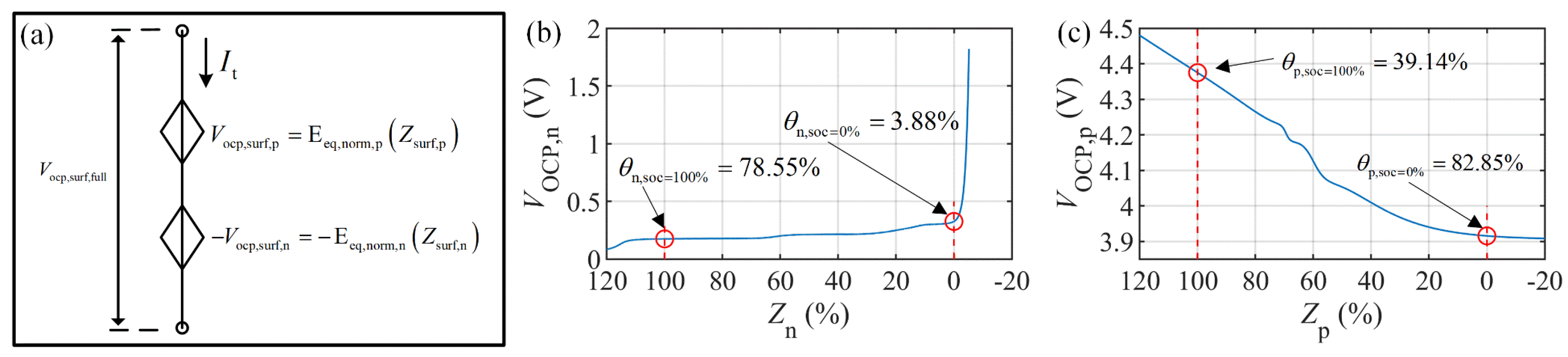
| Relationship between the OCP and normalized SOC of solid particle in positive electrode: | Equation (57) | Figure 8b | ||
| Relationship between the OCP and normalized SOC of solid particle in negative electrode: | Equation (57) | Figure 8c |
| Test Name | SOC Range (%) | R0 (Ω) | R1 (Ω) | C1 (F) | R2 (Ω) | C2 (F) | RMSE of ECM2RC (mV) | RMSE of ECMIESP (mV) |
|---|---|---|---|---|---|---|---|---|
| MHPPC1 | [100, 90] | 0.0381 | 0.0102 | 2133 | 0.0025 | 54,471 | 1.1 | 0.7 |
| MHPPC2 | [90, 80] | 0.0372 | 0.0097 | 2214 | 0.0028 | 29,773 | 1.0 | 0.7 |
| MHPPC3 | [80, 70] | 0.0367 | 0.0079 | 1965 | 0.0061 | 22,776 | 3.8 | 0.8 |
| MHPPC4 | [70, 60] | 0.0370 | 0.0071 | 833 | 0.0159 | 5148 | 6.1 | 0.8 |
| MHPPC5 | [60, 50] | 0.0372 | 0.0136 | 1174 | 0.0010 | 297,555 | 6.9 | 0.7 |
| MHPPC6 | [50, 40] | 0.0372 | 0.0110 | 2494 | 0.0022 | 378,628 | 1.2 | 0.8 |
| MHPPC7 | [40, 30] | 0.0381 | 0.0112 | 2618 | 0.0049 | 181,263 | 2.1 | 0.8 |
| MHPPC8 | [30, 20] | 0.0395 | 0.0166 | 1981 | 0.0098 | 86,366 | 4.2 | 0.8 |
| MHPPC9 | [20, 10] | 0.0418 | 0.0176 | 1651 | 0.0070 | 37,613 | 5.3 | 0.7 |
| MHPPC10 | [10, 0] | 0.0463 | 0.0171 | 2948 | 0.0334 | 26,891 | 60.1 | 1.2 |
| 0.25C Pulse | 0.5C Pulse | 1C Pulse | 2C Pulse | 3C Pulse | 4C Pulse | 5C Pulse | |
|---|---|---|---|---|---|---|---|
| ECM2RC | 0.62 mV | 1.18 mV | 1.61 mV | 5.46 mV | 16.32 mV | 31.71 mV | 50.30 mV |
| ECMIESP | 0.21 mV | 0.41 mV | 0.86 mV | 1.94 mV | 3.00 mV | 4.04 mV | 4.89 mV |
| SOC Range (%) | ECM2RC | ECMIESP | |||
|---|---|---|---|---|---|
| RMSE (mV) | MAXE (mV) | RMSE (mV) | MAXE (mV) | ||
| High SOC segment | [100, 80] | 1.7 | 2.6 | 3.1 | 5.0 |
| Medium SOC segment | [80, 10] | 15.5 | 30.6 | 6.9 | 16.7 |
| Low SOC segment | [10, 0] | 254.5 | 831.0 | 5.4 | 10.8 |
| SOC Range (%) | ECM2RC | ECMIESP | |||
|---|---|---|---|---|---|
| RMSE (mV) | MAXE (mV) | RMSE (mV) | MAXE (mV) | ||
| High SOC segment | [100, 80] | 2.8 | 21.5 | 1.8 | 3.8 |
| Medium SOC segment | [80, 10] | 12.4 | 33.6 | 4.0 | 14.2 |
| Low SOC segment | [10, 0] | 73.4 | 704.7 | 7.0 | 64.3 |
| SOC Range (%) | ECM2RC | ECMIESP | |||
|---|---|---|---|---|---|
| MAXE in CCD | MAXE in HWFET | MAXE in CCD | MAXE in HWFET | ||
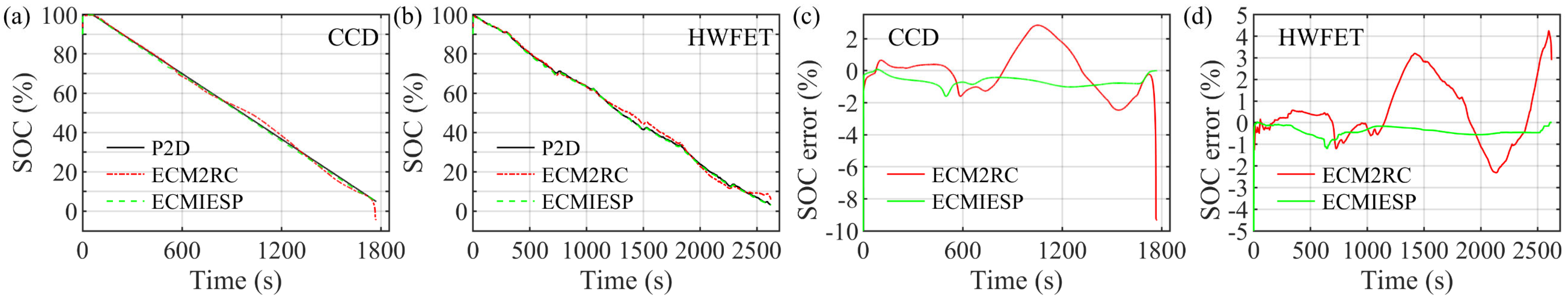
| High SOC segment | [95, 80] | 0.4% | 0.6% | 0.8% | 0.6% |
| Medium SOC segment | [80, 10] | 2.8% | 3.2% | 1.6% | 1.2% |
| Low SOC segment | [10, 0] | 9.4% | 4.3% | 0.7% | 0.5% |
Disclaimer/Publisher’s Note: The statements, opinions and data contained in all publications are solely those of the individual author(s) and contributor(s) and not of MDPI and/or the editor(s). MDPI and/or the editor(s) disclaim responsibility for any injury to people or property resulting from any ideas, methods, instructions or products referred to in the content. |
© 2024 by the authors. Licensee MDPI, Basel, Switzerland. This article is an open access article distributed under the terms and conditions of the Creative Commons Attribution (CC BY) license (https://creativecommons.org/licenses/by/4.0/).
Share and Cite
Li, Y.; Qi, H.; Shi, X.; Jian, Q.; Lan, F.; Chen, J. A Physics-Based Equivalent Circuit Model and State of Charge Estimation for Lithium-Ion Batteries. Energies 2024, 17, 3782. https://doi.org/10.3390/en17153782
Li Y, Qi H, Shi X, Jian Q, Lan F, Chen J. A Physics-Based Equivalent Circuit Model and State of Charge Estimation for Lithium-Ion Batteries. Energies. 2024; 17(15):3782. https://doi.org/10.3390/en17153782
Chicago/Turabian StyleLi, Yigang, Hongzhong Qi, Xinglei Shi, Qifei Jian, Fengchong Lan, and Jiqing Chen. 2024. "A Physics-Based Equivalent Circuit Model and State of Charge Estimation for Lithium-Ion Batteries" Energies 17, no. 15: 3782. https://doi.org/10.3390/en17153782