
A Multiparadigm Approach for Generation Dispatch Optimization in a Regulated Electricity Market towards Clean Energy Transition


 , and
, and
Abstract
1. Introduction
2. Literature Review
2.1. Multiparadigm Approach
2.2. System Dynamics Paradigm
2.3. Multi-Agent System Paradigm
2.4. Generation Dispatch Scheduling
2.5. Unit Commitment
2.6. Economic Dispatch
3. Methodology
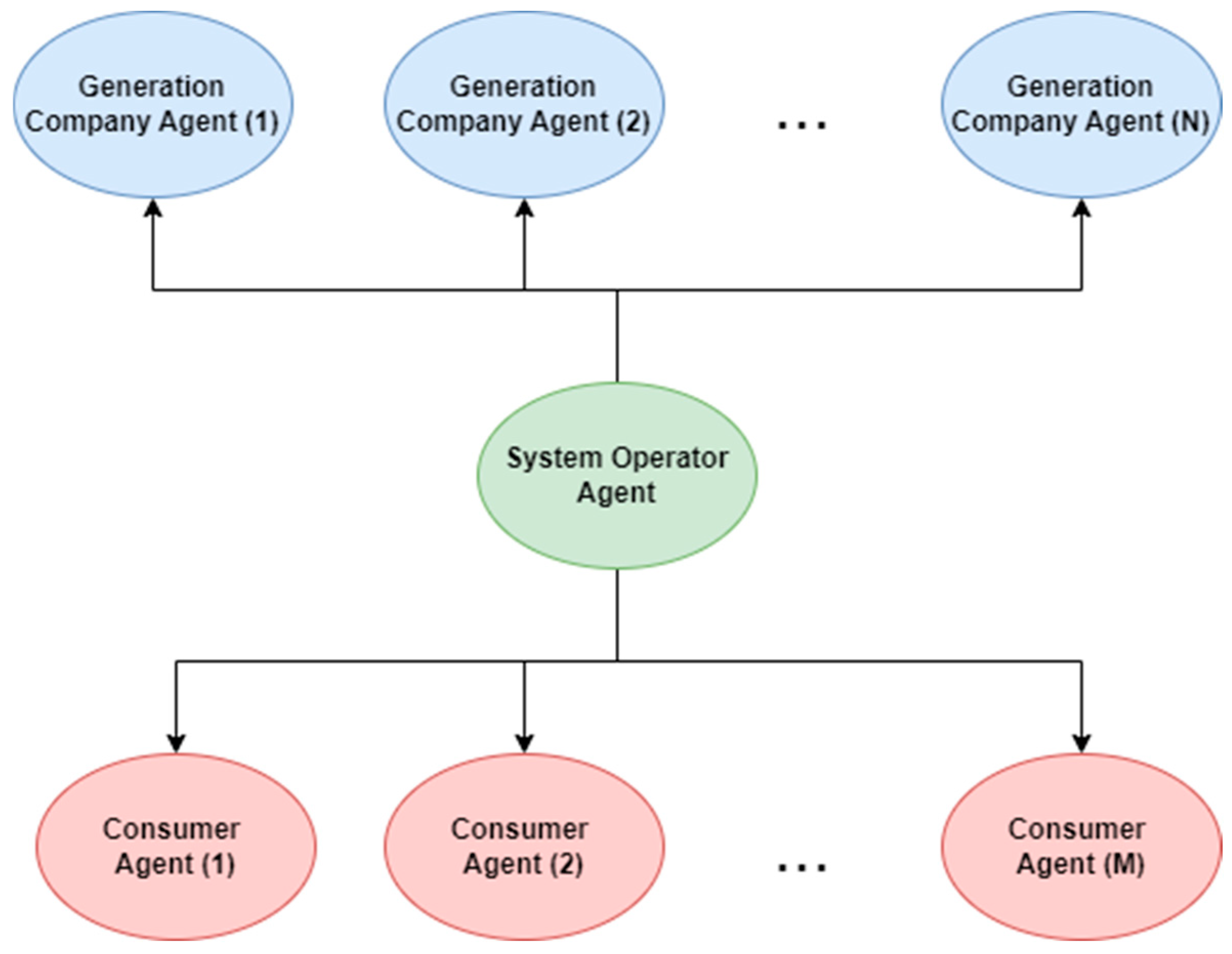
3.1. Multi-Agent System
3.1.1. Generation Company Agent
3.1.2. System Operator Agent
- Total maximum output power represents the total maximum output power of N number of GAs at time t, ensuring the system can meet the maximum (peak) load demands.
- Total minimum output power represents the total minimum output power of N number of GAs at time t. This ensures that there is enough generation to meet the base load without violating any operational constraints.
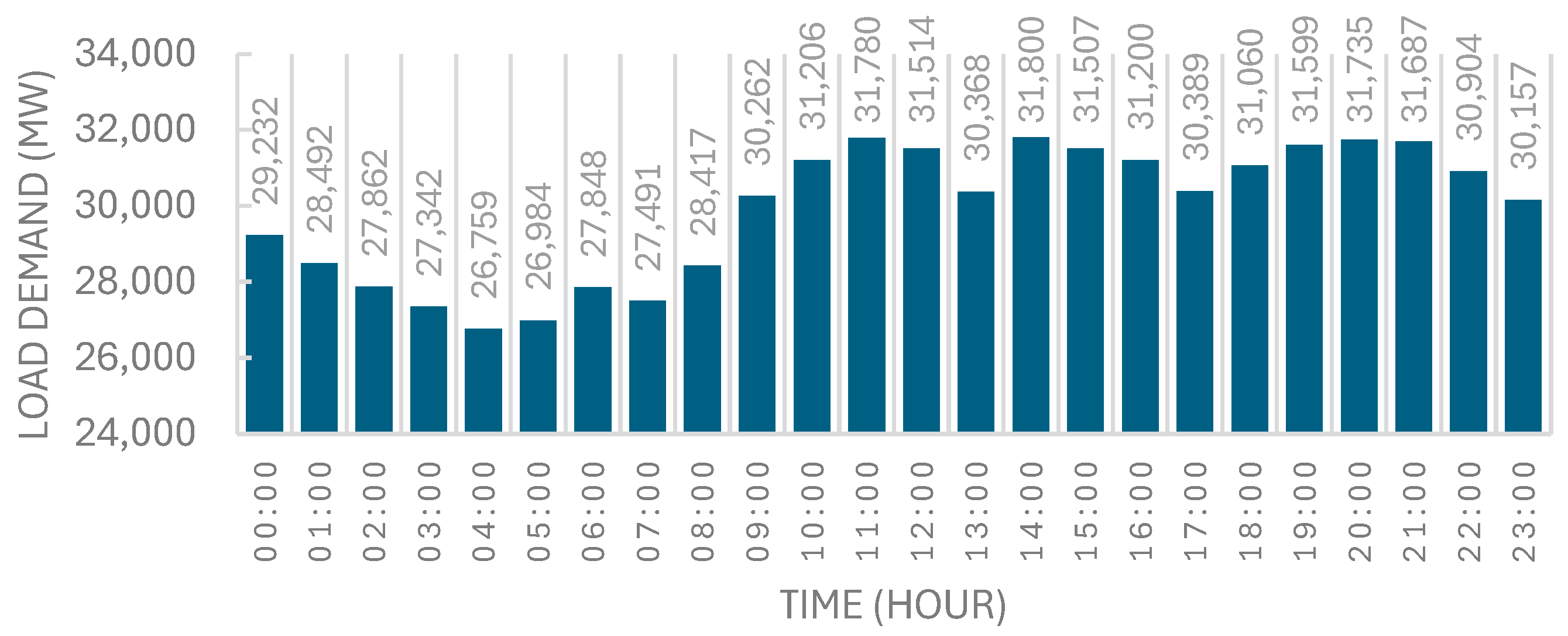
- Total load demand represents the total load demand at time t, wherein the sum of the output powers from the committed GA must match to ensure demand is met.
- Spinning reserve requirement represents the system’s spinning reserve requirement at time t, which is a safety margin to accommodate sudden losses of power supply or unexpected increases in demand.
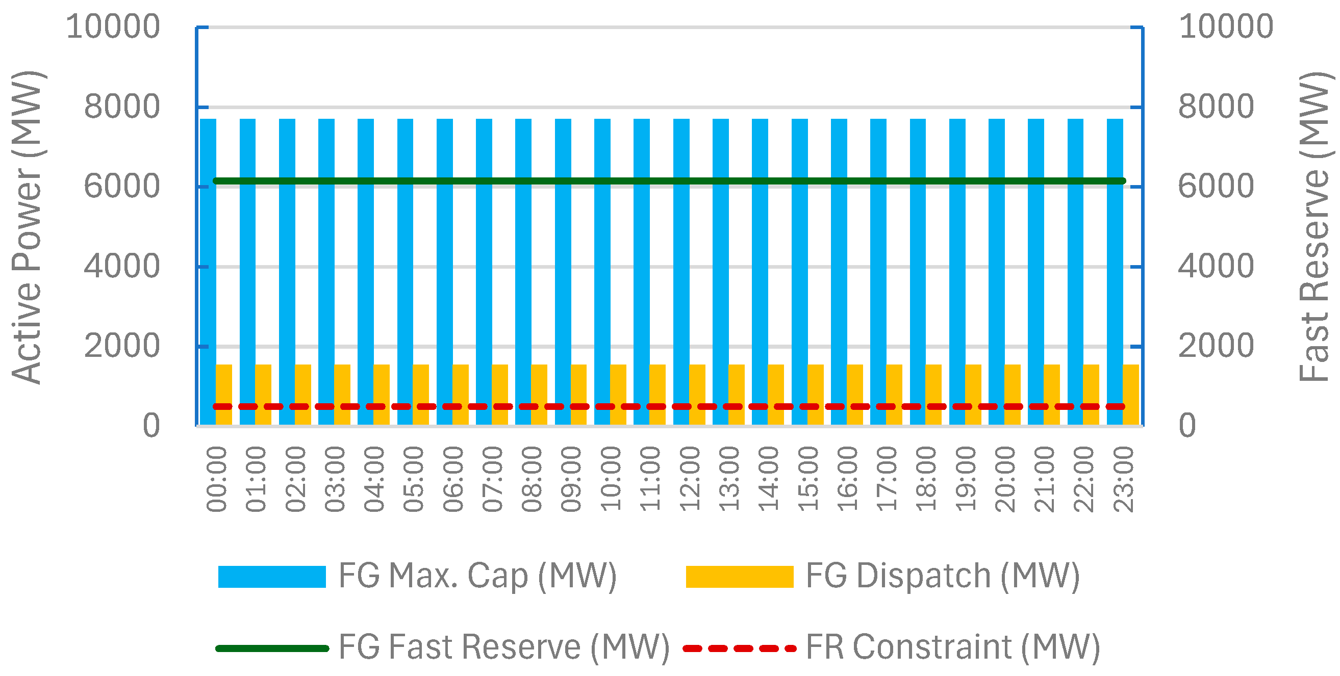
- Power balance constraint, which ensures the total power generated meets the total demand and the system’s fast reserve requirement .
- 2.
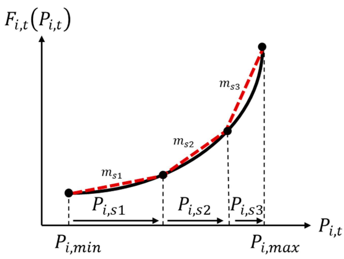
- Generator loading limit constraint, which ensures the output power of each GA in any segment can be maintained within its defined bounds.
3.1.3. Customer Agent
3.2. System Dynamics
- The dispatch flow represents the change in the generator’s power output over time.
- 2.
- The production cost flow is based on the fuel cost function, typically a second-order polynomial with coefficients A, B, and C.
- 3.
- The electricity energy production flow calculates the total energy produced over time.
- 4.
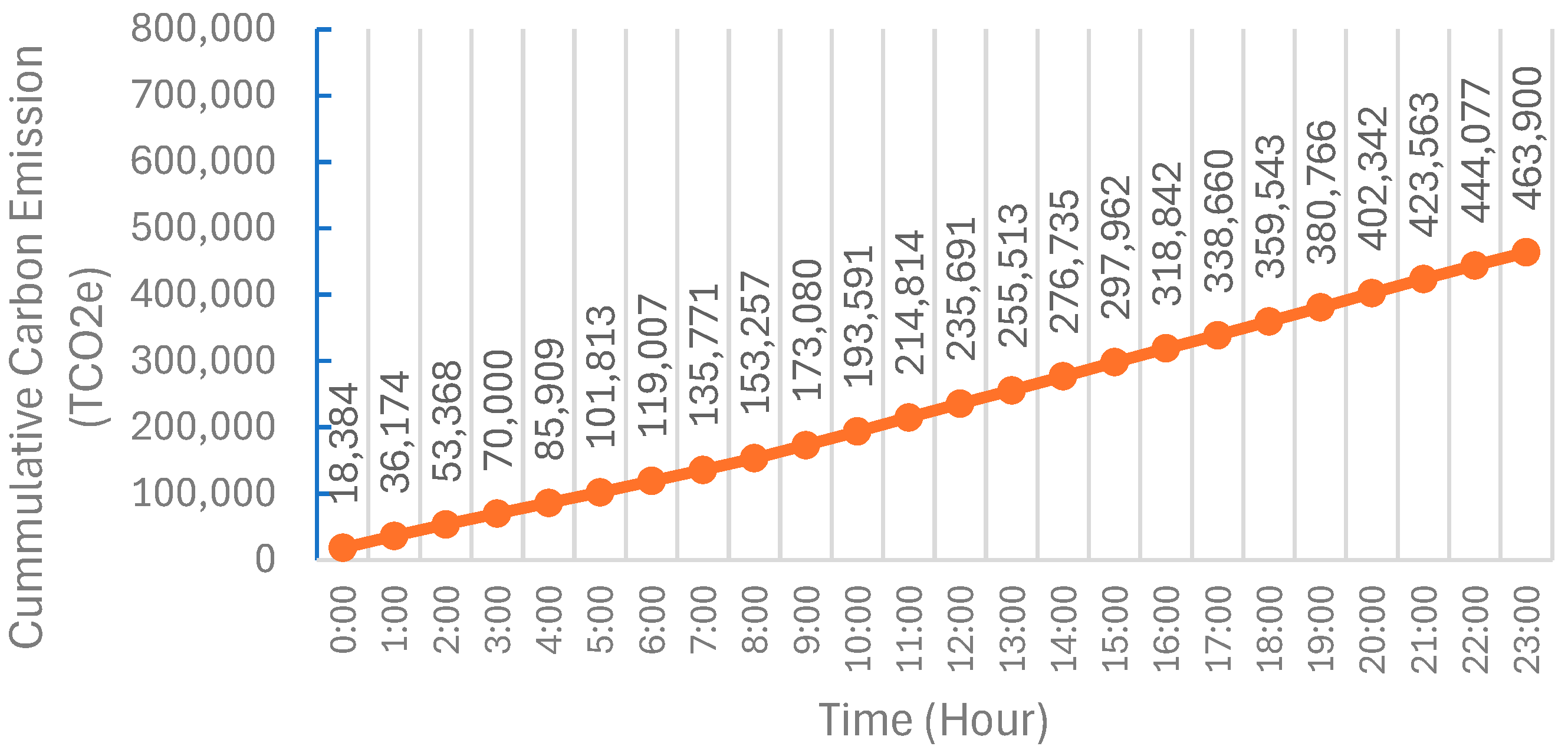
- The carbon emission production flow uses the carbon factor to determine the emissions based on the energy produced.
3.3. Simulation Scenarios
4. Discussion
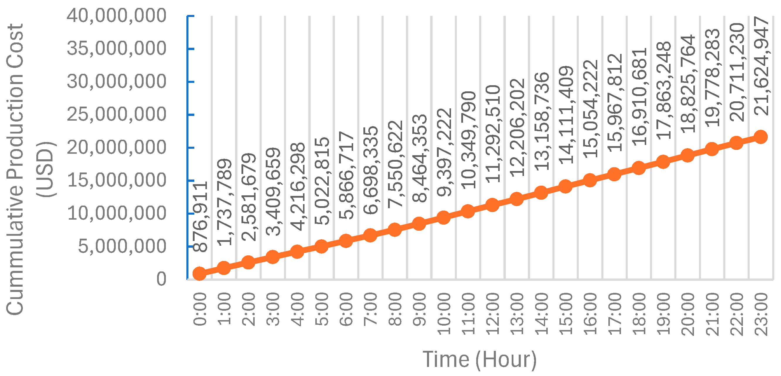
4.1. Base Scenario (Model Validation)
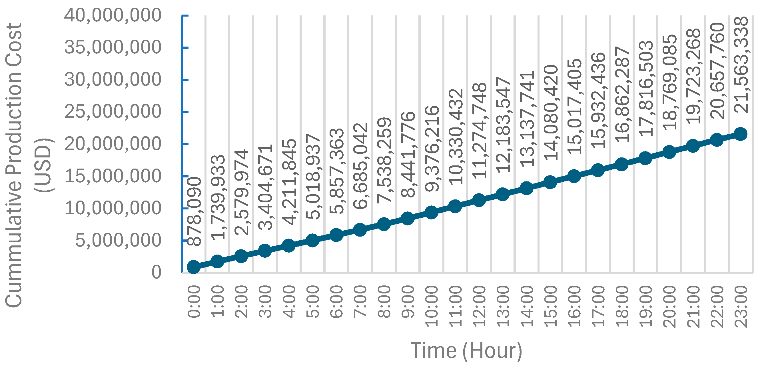
4.2. Carbon Policy Scenarios
4.2.1. Low Carbon Emission Reduction
4.2.2. Moderate Carbon Emission Reduction
4.2.3. High Carbon Emission Reduction
4.2.4. Results Overview
5. Conclusions
Author Contributions
Funding
Data Availability Statement
Acknowledgments
Conflicts of Interest
Abbreviations
| AGC | Automatic generation control |
| AVR | Automatic voltage regulator |
| CA | Consumer agent |
| CFPP | Coal-fired power plant |
| CLD | Causal loop diagram |
| ED | Economic dispatch |
| FACTS | Flexible AC transmission system |
| FG | Frequency governed |
| GA | Generation company agent |
| GS | Generation dispatch scheduling |
| IPP | Independent power producer |
| LP | Linear programming |
| MAS | Multi-agent system |
| PL | Priority list |
| PLN | National utility company |
| PSS | Power system stabilizer |
| SA | System operator agent |
| SD | System dynamics |
| SFD | Stock and flow diagram |
| TCO2e | Tons of carbon emissions |
| UC | Unit commitment |
| VRE | Variable renewable energy |
References
- National Energy Council of Indonesia. Indonesia Energy Outlook. 2023. Available online: https://den.go.id/publikasi/Outlook-Energi-Indonesia (accessed on 17 July 2024).
- International Energy Agency (IEA). An Energy Sector Roadmap to Net Zero Emissions in Indonesia; IEA: Paris, France, 2022. [Google Scholar]
- LV, G.; Cao, B.; Jun, L.; Liu, G.; Ding, Y.; Yu, J.; Zang, Y.; Zhang, D. Optimal Scheduling of Integrated Energy System under the Background of Carbon Neutrality. Energy Rep. 2022, 8, 1236–1248. [Google Scholar] [CrossRef]
- Logenthiran, T.; Srinivasan, D.; Khambadkone, A.M.; Aung, H.N. Multi-Agent System (MAS) for Short-Term Generation Scheduling of a Microgrid. In Proceedings of the 2010 IEEE International Conference on Sustainable Energy Technologies (ICSET), Kandy, Sri Lanka, 6–9 December 2010; pp. 1–6. [Google Scholar]
- Alam, M.S.; Hari Kiran, B.D.; Kumari, M.S. Priority List and Particle Swarm Optimization Based Unit Commitment of Thermal Units Including Renewable Uncertainties. In Proceedings of the 2016 IEEE International Conference on Power System Technology (POWERCON), Wollongong, NSW, Australia, 28 September–1 October 2016; pp. 1–6. [Google Scholar]
- Efecik, K.; Wang, X. Economic Dispatch of Energy Storage Systems for Smart Power Grid. In Proceedings of the 2023 IEEE Transportation Electrification Conference & Expo (ITEC), Detroit, MI, USA, 21–23 June 2023; pp. 1–4. [Google Scholar]
- Grond, M.O.W.; Luong, N.H.; Morren, J.; Slootweg, J.G. Multi-Objective Optimization Techniques and Applications in Electric Power Systems. In Proceedings of the 2012 47th International Universities Power Engineering Conference (UPEC), Uxbridge, UK, 4–7 September 2012; pp. 1–6. [Google Scholar]
- To, L.S.; Bruce, A.; Munro, P.; Santagata, E.; MacGill, I.; Rawali, M.; Raturi, A. A Research and Innovation Agenda for Energy Resilience in Pacific Island Countries and Territories. Nat. Energy 2021, 6, 1098–1103. [Google Scholar] [CrossRef]
- Psarros, G.N.; Papathanassiou, S.A. Generation Scheduling in Island Systems with Variable Renewable Energy Sources: A Literature Review. Renew. Energy 2023, 205, 1105–1124. [Google Scholar] [CrossRef]
- Liu, Z.-F.; Li, L.-L.; Liu, Y.-W.; Liu, J.-Q.; Li, H.-Y.; Shen, Q. Dynamic Economic Emission Dispatch Considering Renewable Energy Generation: A Novel Multi-Objective Optimization Approach. Energy 2021, 235, 121407. [Google Scholar] [CrossRef]
- Manfren, M.; Caputo, P.; Costa, G. Paradigm Shift in Urban Energy Systems through Distributed Generation: Methods and Models. Appl. Energy 2011, 88, 1032–1048. [Google Scholar] [CrossRef]
- Quiroga, M.A.; Franco, A.A. A Multi-Paradigm Computational Model of Materials Electrochemical Reactivity for Energy Conversion and Storage. J. Electrochem. Soc. 2015, 162, E73–E83. [Google Scholar] [CrossRef]
- Carreira, P.; Amaral, V.; Vangheluwe, H. Multi-Paradigm Modelling for Cyber-Physical Systems: Foundations. In Foundations of Multi-Paradigm Modelling for Cyber-Physical Systems; Springer International Publishing: Cham, Switzerland, 2020; pp. 1–14. ISBN 9783030439460. [Google Scholar]
- Marzbani, F.; Abdelfatah, A. Economic Dispatch Optimization Strategies and Problem Formulation: A Comprehensive Review. Energies 2024, 17, 550. [Google Scholar] [CrossRef]
- Pamulapati, T.; Cavus, M.; Odigwe, I.; Allahham, A.; Walker, S.; Giaouris, D. A Review of Microgrid Energy Management Strategies from the Energy Trilemma Perspective. Energies 2022, 16, 289. [Google Scholar] [CrossRef]
- Talukdar, S. Multi-Agent Systems. In Proceedings of the IEEE Power Engineering Society General Meeting, Orlando, FL, USA, 16–20 July 2023; Volume 2, pp. 59–60. [Google Scholar]
- Kazmi, S.A.A.; Khan, U.A.; Ahmad, H.W.; Ali, S.; Shin, D.R. A Techno-Economic Centric Integrated Decision-Making Planning Approach for Optimal Assets Placement in Meshed Distribution Network across the Load Growth. Energies 2020, 13, 1444. [Google Scholar] [CrossRef]
- Azar, A.T. System Dynamics as a Useful Technique for Complex Systems. Int. J. Ind. Syst. Eng. 2012, 10, 377–410. [Google Scholar] [CrossRef]
- Parker, D.C.; Manson, S.M.; Janssen, M.A.; Hoffmann, M.J.; Deadman, P. Multi-Agent Systems for the Simulation of Land-Use and Land-Cover Change: A Review. Ann. Assoc. Am. Geogr. 2003, 93, 314–337. [Google Scholar] [CrossRef]
- Borshchev, A.; Filippov, A. From System Dynamics and Discrete Even to Practical Agent Based Modeling. In Proceedings of the The 22nd International Conference of the System Dynamics Society, Oxford, UK, 25–29 July 2004. [Google Scholar]
- Nair, K.; Shadman, S.; Chin, C.M.M.; Sakundarini, N.; Yap, E.H.; Koyande, A. Developing a System Dynamics Model to Study the Impact of Renewable Energy in the Short- and Long-Term Energy Security. Mater. Sci. Energy Technol. 2021, 4, 391–397. [Google Scholar] [CrossRef]
- De Marco, A.; Fakhry, H.; Postorino, M.; Mammar, Z.; Hacid, H. System Dynamics Modeling of Logistics Hub Capacity: The Dubai Logistics Corridor Case Study. In Proceedings of the Dynamics in Logistics; Freitag, M., Haasis, H.-D., Kotzab, H., Pannek, J., Eds.; Springer International Publishing: Cham, Switzerland, 2020; pp. 21–31. [Google Scholar]
- Teng, J.; Xu, C.; Wang, W.; Wu, X. A System Dynamics-Based Decision-Making Tool and Strategy Optimization Simulation of Green Building Development in China. Clean. Technol. Environ. Policy 2018, 20, 1259–1270. [Google Scholar] [CrossRef]
- Ding, Z.; Gong, W.; Li, S.; Wu, Z. System Dynamics versus Agent-Based Modeling: A Review of Complexity Simulation in Construction Waste Management. Sustainability 2018, 10, 2484. [Google Scholar] [CrossRef]
- Sterman, J.D. Learning in and about Complex Systems. Syst. Dyn. Rev. 1994, 10, 291–330. [Google Scholar] [CrossRef]
- Fang, X.; Wang, J.; Song, G.; Han, Y.; Zhao, Q.; Cao, Z. Multi-Agent Reinforcement Learning Approach for Residential Microgrid Energy Scheduling. Energies 2019, 13, 123. [Google Scholar] [CrossRef]
- Loo, Y.L.; Tang, A.Y.C.; Ahmad, A. Identifying Key Factors in Agent-Based Simulation Model on Processes in Time-Constrained Environment. In Proceedings of the 2015 International Symposium on Agents, Multi-Agent Systems and Robotics (ISAMSR), Putrajaya, Malaysia, 18–19 August 2015; pp. 71–76. [Google Scholar]
- Ross, W.; Ulieru, M.; Gorod, A. A Multi-Paradigm Modelling & Simulation Approach for System of Systems Engineering: A Case Study. In Proceedings of the 2014 9th International Conference on System of Systems Engineering (SOSE), Glenelg, SA, Australia, 9–13 June 2014; pp. 183–188. [Google Scholar]
- Lez-Briones, A.G.; De La Prieta, F.; Mohamad, M.S.; Omatu, S.; Corchado, J.M. Multi-Agent Systems Applications in Energy Optimization Problems: A State-of-the-Art Review. Energies 2018, 11, 1928. [Google Scholar] [CrossRef]
- Halinka, A.; Rzepka, P.; Szablicki, M. Agent Model of Multi-Agent System for Area Power System Protection. In Proceedings of the 2015 Modern Electric Power Systems (MEPS), Wroclaw, Poland, 6–9 July 2015; pp. 1–4. [Google Scholar]
- Wu, N.; Zhou, X.; Sun, M. Incentive Mechanisms and Impacts of Negotiation Power and Information Availability in Multi-Relay Cooperative Wireless Networks. IEEE Trans. Wirel. Commun. 2019, 18, 3752–3765. [Google Scholar] [CrossRef]
- Wang, J.; Wu, J.; Kong, X. Multi-Agent Simulation for Strategic Bidding in Electricity Markets Using Reinforcement Learning. CSEE J. Power Energy Syst. 2023, 9, 1051–1065. [Google Scholar] [CrossRef]
- Yin, B.; Weng, H.; Hu, Y.; Xi, J.; Ding, P.; Liu, J. Multi-Agent Deep Reinforcement Learning for Simulating Centralized Double-Sided Auction Electricity Market. IEEE Trans. Power Syst. 2024, 1–12. [Google Scholar] [CrossRef]
- Manjunatha, H.M.; Purushothama, G.K.; Nanjappa, Y.; Deshpande, R. Auction-Based Single-Sided Bidding Electricity Market: An Alternative to the Bilateral Contractual Energy Trading Model in a Grid-Tied Microgrid. IEEE Access 2024, 12, 48975–48986. [Google Scholar] [CrossRef]
- Zhao, C.; Sun, J.; He, P. Bidding Strategies and Equilibrium Analysis in Electricity Market under RPS and CET. In Proceedings of the 2023 IEEE 7th Conference on Energy Internet and Energy System Integration (EI2), Hangzhou, China, 15–18 December 2023; pp. 3142–3147. [Google Scholar]
- Ren, D.; Guo, X. Simulation Modeling and Analysis of Carbon Emission Reduction Potential of Multi-Energy Generation. Environ. Dev. Sustain. 2023, 25, 11823–11845. [Google Scholar] [CrossRef]
- Ebrie, A.S.; Kim, Y.J. Reinforcement Learning-Based Multi-Objective Optimization for Generation Scheduling in Power Systems. Systems 2024, 12, 106. [Google Scholar] [CrossRef]
- Kaur, G.; Dhillon, J.S. Electricity Generation Scheduling of Thermal-Wind-Solar Energy Systems. Electr. Eng. 2023, 105, 3549–3579. [Google Scholar] [CrossRef]
- Salkuti, S.R. Day-Ahead Thermal and Renewable Power Generation Scheduling Considering Uncertainty. Renew. Energy 2019, 131, 956–965. [Google Scholar] [CrossRef]
- Xu, Y.; Wang, Z.; Sun, W.; Chen, S.; Wu, Y.; Zhao, B. Unit Commitment Model Considering Nuclear Power Plant Load Following. In Proceedings of the 2011 International Conference on Advanced Power System Automation and Protection, Beijing, China, 16–20 October 2011; Volume 3, pp. 1828–1832. [Google Scholar]
- Benhamida, F.; Abdelbar, B. Enhanced Lagrangian Relaxation Solution to the Generation Scheduling Problem. Int. J. Electr. Power Energy Syst. 2010, 32, 1099–1105. [Google Scholar] [CrossRef]
- Elsayed, A.M.; Maklad, A.M.; Farrag, S.M. A New Priority List Unit Commitment Method for Large-Scale Power Systems. In Proceedings of the 2017 Nineteenth International Middle East Power Systems Conference (MEPCON), Cairo, Egypt, 19–21 December 2017; pp. 359–367. [Google Scholar]
- Wang, T.; Hua, H.; Shi, T.; Wang, R.; Sun, Y.; Naidoo, P. A Bi-Level Dispatch Optimization of Multi-Microgrid Considering Green Electricity Consumption Willingness under Renewable Portfolio Standard Policy. Appl. Energy 2024, 356, 122428. [Google Scholar] [CrossRef]
- Wu, Y.K.; Huang, C.-C.; Lin, C.-L.; Chang, S.-M. A Hybrid Unit Commitment Approach Incorporating Modified Priority List with Charged System Search Methods. Smart Grid Renew. Energy 2017, 8, 178–194. [Google Scholar] [CrossRef]
- Srinivasan, D.; Chazelas, J. A Priority List-Based Evolutionary Algorithm to Solve Large Scale Unit Commitment Problem. In Proceedings of the 2004 International Conference on Power System Technology, 2004. PowerCon 2004, Singapore, 21–24 November 2004; Volume 2, pp. 1746–1751. [Google Scholar]
- Kazarlis, S.A.; Bakirtzis, A.G.; Petridis, V. A Genetic Algorithm Solution to the Unit Commitment Problem. IEEE Trans. Power Syst. 1996, 11, 83–92. [Google Scholar] [CrossRef]
- Juste, K.A.; Kita, H.; Tanaka, E.; Hasegawa, J. An Evolutionary Programming Solution to the Unit Commitment Problem. IEEE Trans. Power Syst. 1999, 14, 1452–1459. [Google Scholar] [CrossRef]
- Senjyu, T.; Shimabukuro, K.; Uezato, K.; Funabashi, T. A Fast Technique for Unit Commitment Problem by Extended Priority List. IEEE Trans. Power Syst. 2003, 18, 882–888. [Google Scholar] [CrossRef]
- Kunya, A.; Abubakar, A.S.; Yusuf, S. Review of Economic Dispatch in Multi-Area Power System: State-of-the-Art and Future Prospective. Electr. Power Syst. Res. 2023, 217, 109089. [Google Scholar] [CrossRef]
- Luo, Z.; Wang, J.; Xiao, N.; Yang, L.; Zhao, W.; Geng, J.; Lu, T.; Luo, M.; Dong, C. Low Carbon Economic Dispatch Optimization of Regional Integrated Energy Systems Considering Heating Network and P2G. Energies 2022, 15, 5494. [Google Scholar] [CrossRef]
- Javadi, M.; Amraee, T. Economic Dispatch: A Mixed-Integer Linear Model for Thermal Generating Units. In Proceedings of the 2018 IEEE International Conference on Environment and Electrical Engineering and 2018 IEEE Industrial and Commercial Power Systems Europe (EEEIC/I&CPS Europe), Palermo, Italy, 12–15 June 2018; pp. 1–5. [Google Scholar]
- Nemati, M.; Braun, M.; Tenbohlen, S. Optimization of Unit Commitment and Economic Dispatch in Microgrids Based on Genetic Algorithm and Mixed Integer Linear Programming. Appl. Energy 2018, 210, 944–963. [Google Scholar] [CrossRef]
- Ministry of Mineral Energy and Resources National Electricity Supply Business Plan 2021–2030. Available online: https://web.pln.co.id/stakeholder/ruptl (accessed on 12 July 2024).
- PT PLN (Persero)—Pusat Pengatur Beban. Fast Response Generator in Java-Madura-Bali Power System 2023; PT PLN (Persero): Jakarta, Indonesia, 2023. [Google Scholar]
- PT PLN (Persero)—Pusat Pengatur Beban. Carbon Factor Data for Thermal Power Plants in Java-Madura-Bali Power System 2023; PT PLN (Persero): Jakarta, Indonesia, 2023. [Google Scholar]
- Power Generation, Operation, and Control, 3rd ed.; Wiley-Interscience: Hoboken, NJ, USA, 2014.
- Sarjiya; Mulyawan, A.B.; Setiawan, A.; Sudiarso, A. Thermal Unit Commitment Solution Using Genetic Algorithm Combined with the Principle of Tabu Search and Priority List Method. In Proceedings of the 2013 International Conference on Information Technology and Electrical Engineering (ICITEE), Yogyakarta, Indonesia, 7–8 October 2013; pp. 414–419. [Google Scholar]
- Abou El-Ela, A.A.; Allam, S.M.; Rizk-Allah, R.M.; Doso, A.S. Parallel Binary Sine Cosine with Optimal Priority List Algorithm for Unit Commitment. In Proceedings of the 2019 21st International Middle East Power Systems Conference (MEPCON), Cairo, Egypt, 17–19 December 2019; pp. 509–514. [Google Scholar]
- PT PLN (Persero)—Pusat Pengatur Beban. Daily Load Curve of Java-Madura-Bali Power System 2023; PT PLN (Persero): Jakarta, Indonesia, 2023. [Google Scholar]
- Indonesia Solar Map. Java-Madura-Bali Irradiation Data in June 2023. Available online: https://indonesiasolarmap.com/ (accessed on 12 July 2024).


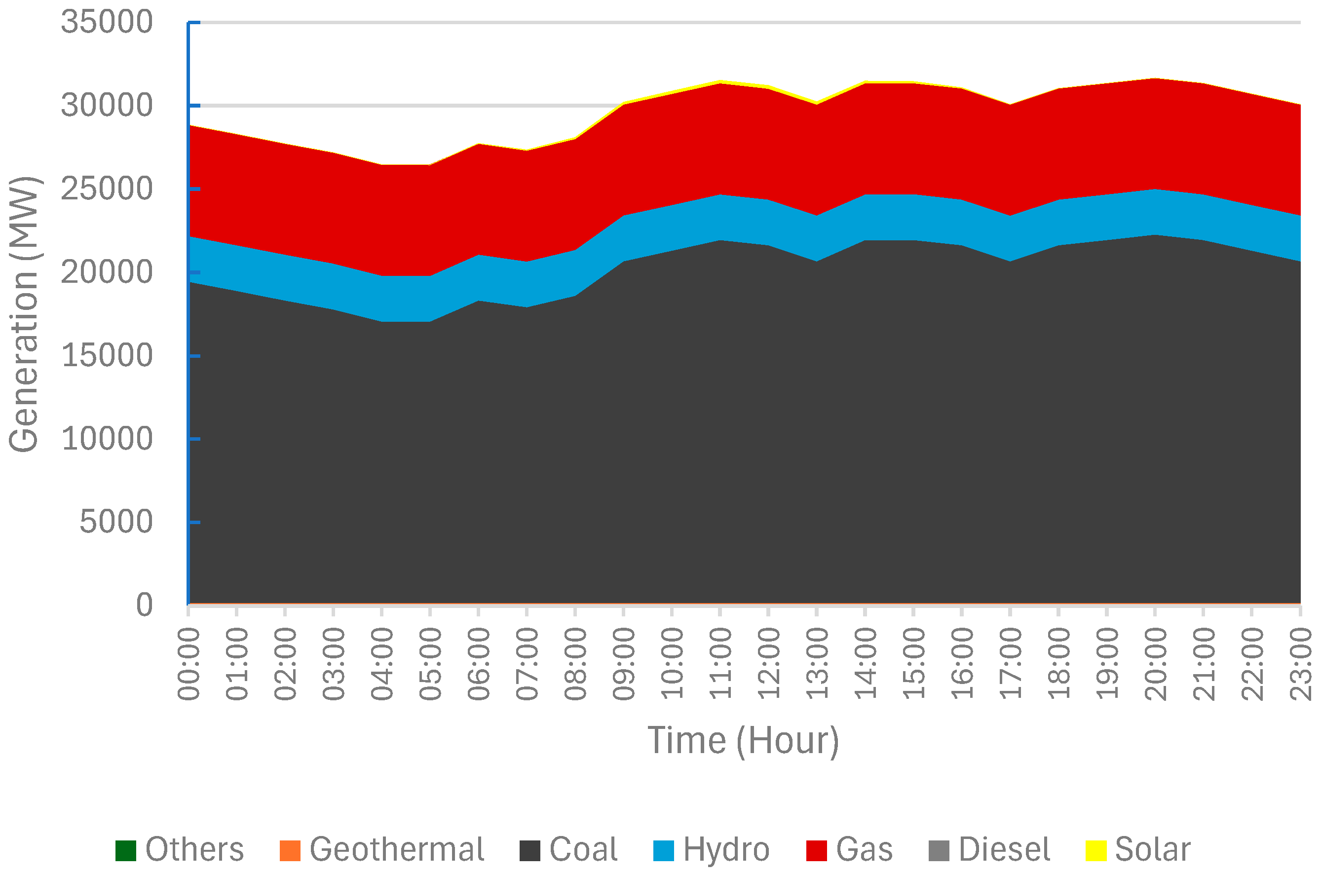
| Generating Unit Category | Number of Unit(s) | Installed Capacity (MW) | Percentage (%) |
|---|---|---|---|
| Geothermal | 19 | 1225 | 2.6% |
| Waste-to-energy and biomass | 4 | 34 | 0.1% |
| Large-scale hydro | 95 | 2616 | 5.5% |
| Small-scale hydro | 40 | 222 | 0.5% |
| Coal-fired | 62 | 28,545 | 60.4% |
| Combined-cycle gas turbine | 87 | 13,965 | 29.5% |
| Open-cycle gas turbine | 9 | 353 | 0.7% |
| Gas engine | 4 | 182 | 0.4% |
| Diesel | 7 | 152 | 0.3% |
| Total | 327 | 47,294 | 100.0% |
| Name | Min. Loading (MW) | Max. Loading (MW) | Fuel Cost Function (Cent/Hour) | ||
|---|---|---|---|---|---|
| Quadratic Coefficient (aP2) | Linear Coefficient (bP) | Constant (c) | |||
| CFPP Jawa-4 Tanjung Jati #1 | 500 | 1000 | 1.80 | −742.63 | 1,248,341.14 |
| Priority List Scheme | Committed Generation Unit | Total Minimum Capacity | Total Maximum Capacity |
|---|---|---|---|
| 1 | |||
| 2 | , | ||
| … | … | … | … |
| N | , , …, |
| Scenario Type | Emission Reduction Objective | Unit |
|---|---|---|
| Base | 0 | TCO2e per day |
| Carbon policy (low) | 5000 | TCO2e per day |
| Carbon policy (moderate) | 10,000 | TCO2e per day |
| Carbon policy (high) | 15,000 | TCO2e per day |
| Parameter | Constraint | Value | Unit |
|---|---|---|---|
| Power mismatch limit | Less than or equal to (≤) | 1.0 | % |
| System spinning reserve | Greater than or equal to (≥) | 1000 | MW |
| System fast reserve | Greater than or equal to (≥) | 500 | MW |
| Output Variables | Unit | Base | Carbon Policy (Low) | Carbon Policy (Moderate) | Carbon Policy (High) |
|---|---|---|---|---|---|
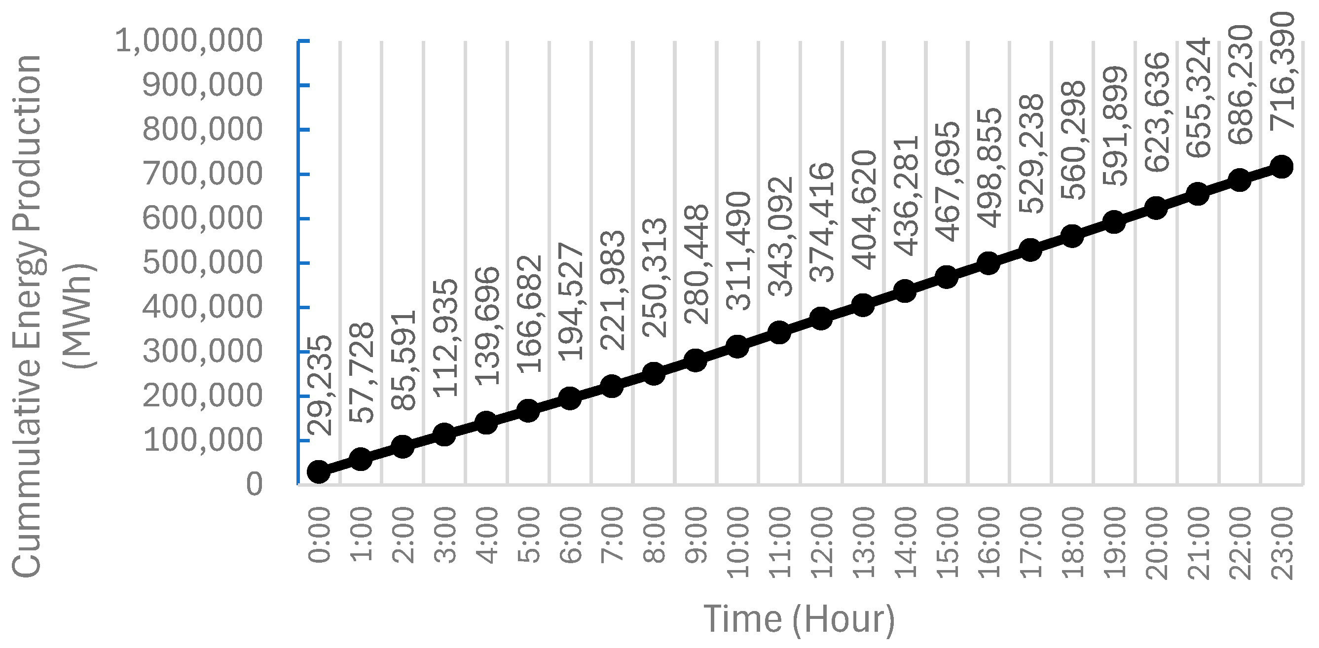
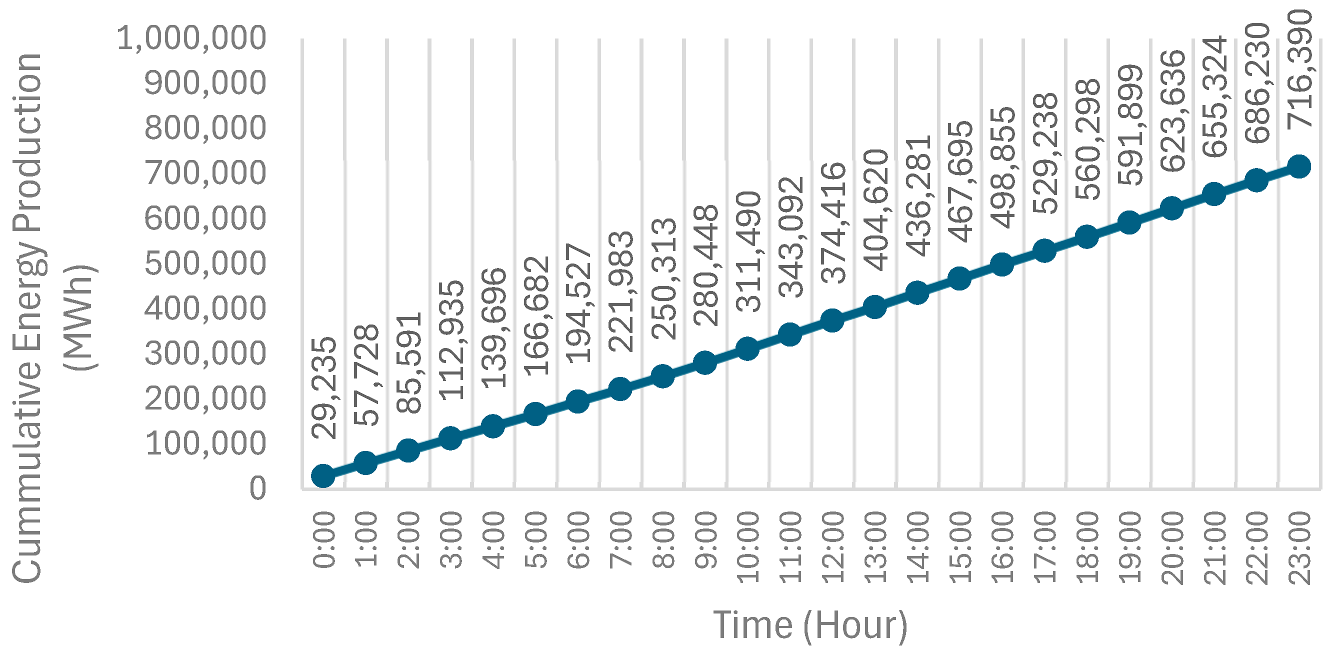
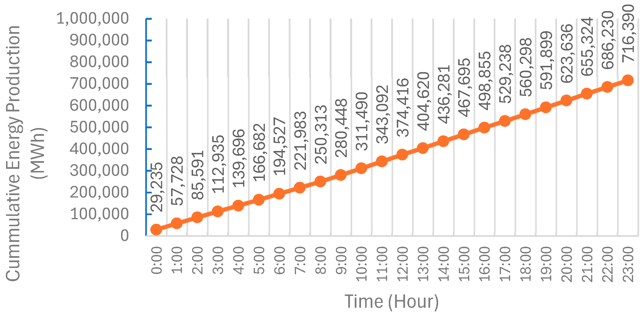
| Total electricity Energy production | MWh | 716,390 | 716,390 | 716,390 | 716,390 |
| Total production (fuel) cost | USD | 21,290,150 | 21,425,290 | 21,563,338 | 21,624,947 |
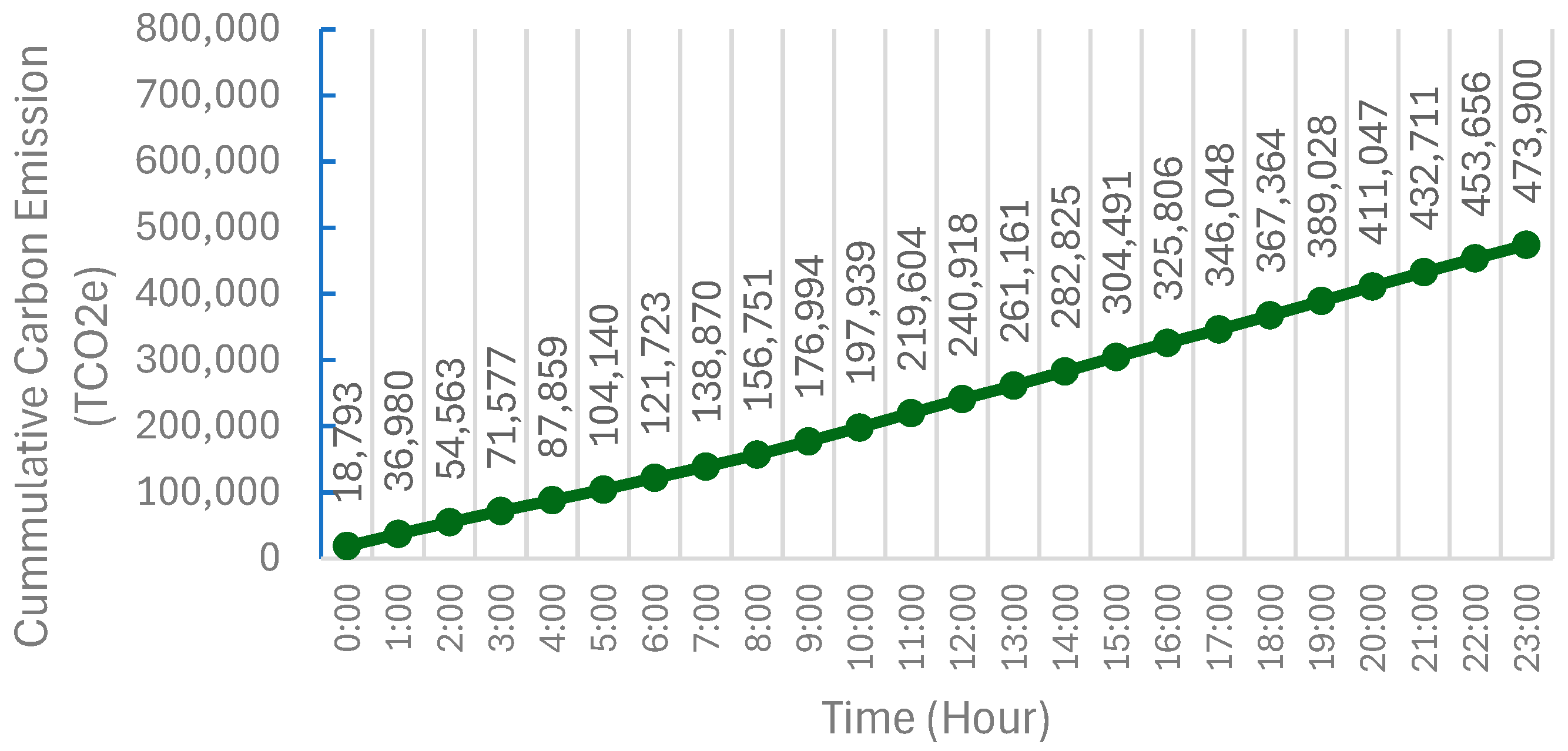
| Total carbon emission production | TCO2e | 478,900 | 473,900 | 468,900 | 463,900 |
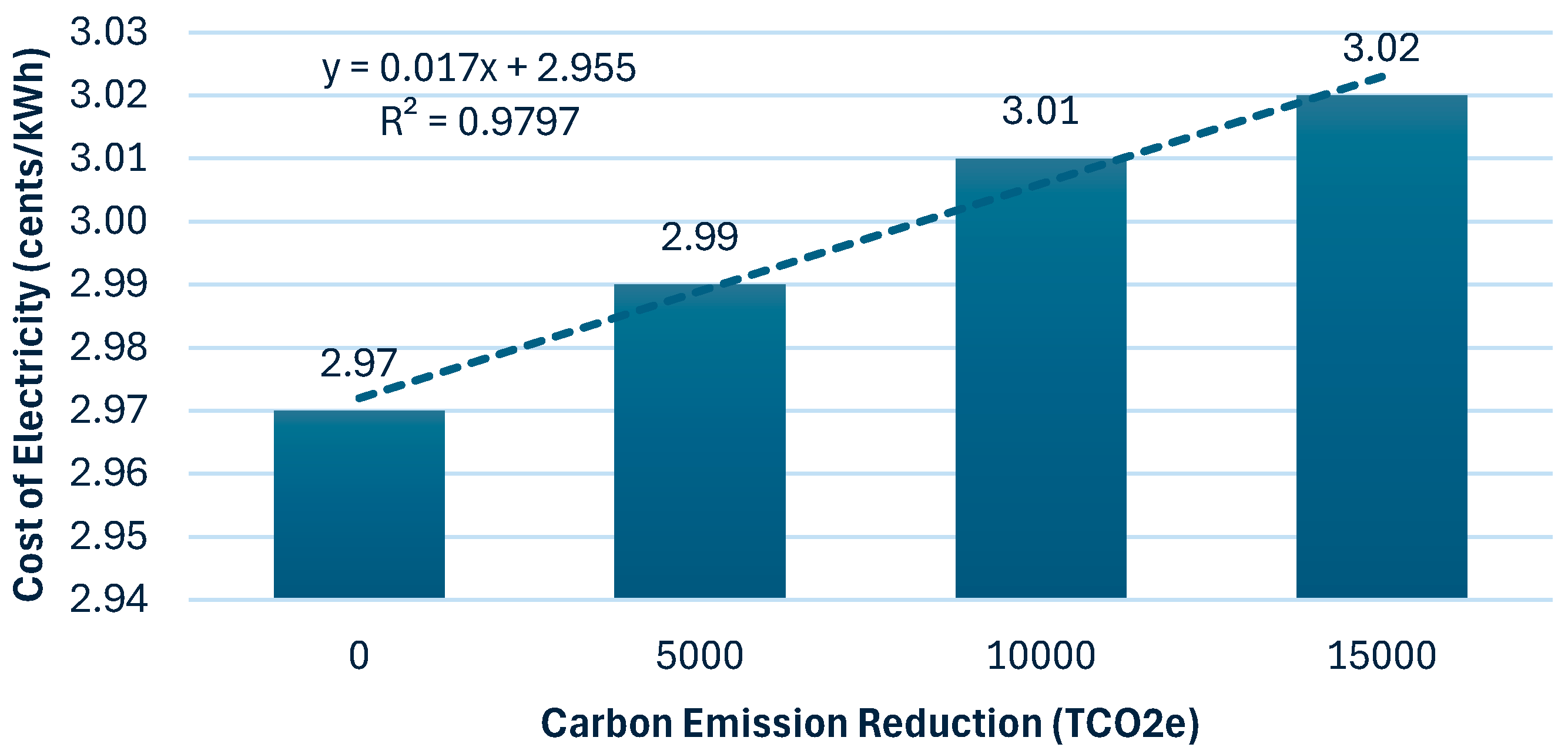
| Carbon emission reduction | TCO2e | 0 | 5000 | 10,000 | 15,000 |
| Cost of electricity | cents/kWh | 2.97 | 2.99 | 3.01 | 3.02 |
Disclaimer/Publisher’s Note: The statements, opinions and data contained in all publications are solely those of the individual author(s) and contributor(s) and not of MDPI and/or the editor(s). MDPI and/or the editor(s) disclaim responsibility for any injury to people or property resulting from any ideas, methods, instructions or products referred to in the content. |
© 2024 by the authors. Licensee MDPI, Basel, Switzerland. This article is an open access article distributed under the terms and conditions of the Creative Commons Attribution (CC BY) license (https://creativecommons.org/licenses/by/4.0/).
Share and Cite
Isnandar, S.; Simorangkir, J.F.; Banjar-Nahor, K.M.; Paradongan, H.T.; Hariyanto, N. A Multiparadigm Approach for Generation Dispatch Optimization in a Regulated Electricity Market towards Clean Energy Transition. Energies 2024, 17, 3807. https://doi.org/10.3390/en17153807
Isnandar S, Simorangkir JF, Banjar-Nahor KM, Paradongan HT, Hariyanto N. A Multiparadigm Approach for Generation Dispatch Optimization in a Regulated Electricity Market towards Clean Energy Transition. Energies. 2024; 17(15):3807. https://doi.org/10.3390/en17153807
Chicago/Turabian StyleIsnandar, Suroso, Jonathan F. Simorangkir, Kevin M. Banjar-Nahor, Hendry Timotiyas Paradongan, and Nanang Hariyanto. 2024. "A Multiparadigm Approach for Generation Dispatch Optimization in a Regulated Electricity Market towards Clean Energy Transition" Energies 17, no. 15: 3807. https://doi.org/10.3390/en17153807
APA StyleIsnandar, S., Simorangkir, J. F., Banjar-Nahor, K. M., Paradongan, H. T., & Hariyanto, N. (2024). A Multiparadigm Approach for Generation Dispatch Optimization in a Regulated Electricity Market towards Clean Energy Transition. Energies, 17(15), 3807. https://doi.org/10.3390/en17153807