

Study of a Numerical Integral Interpolation Method for Electromagnetic Transient Simulations

Abstract
:1. Introduction
- (1)
- L-stable, to effectively eliminate oscillations;
- (2)
- Variable step size, to handle switching events at any time;
- (3)
- High computational accuracy, at least secondary-order, during interpolation;
- (4)
- Consistent equivalent impedance, and the conductivity matrix does not need to re-triangulated;
- (5)
- It is better to construct it on the CDA scheme to minimize modifications of EMT-type tools.
2. Interpolation in CDA and Its Defects
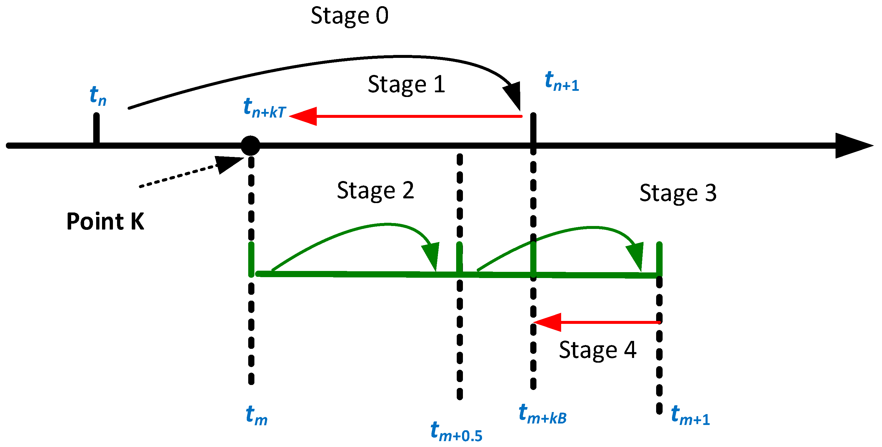
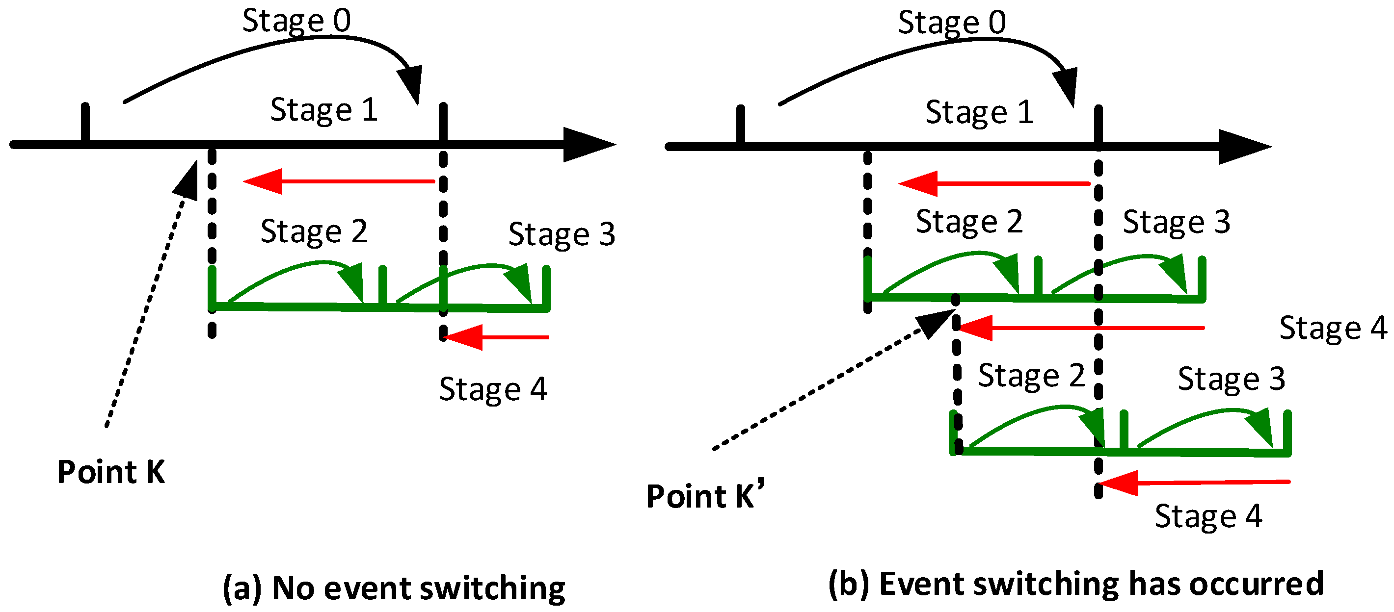
2.1. Switching Interpolation Architecture
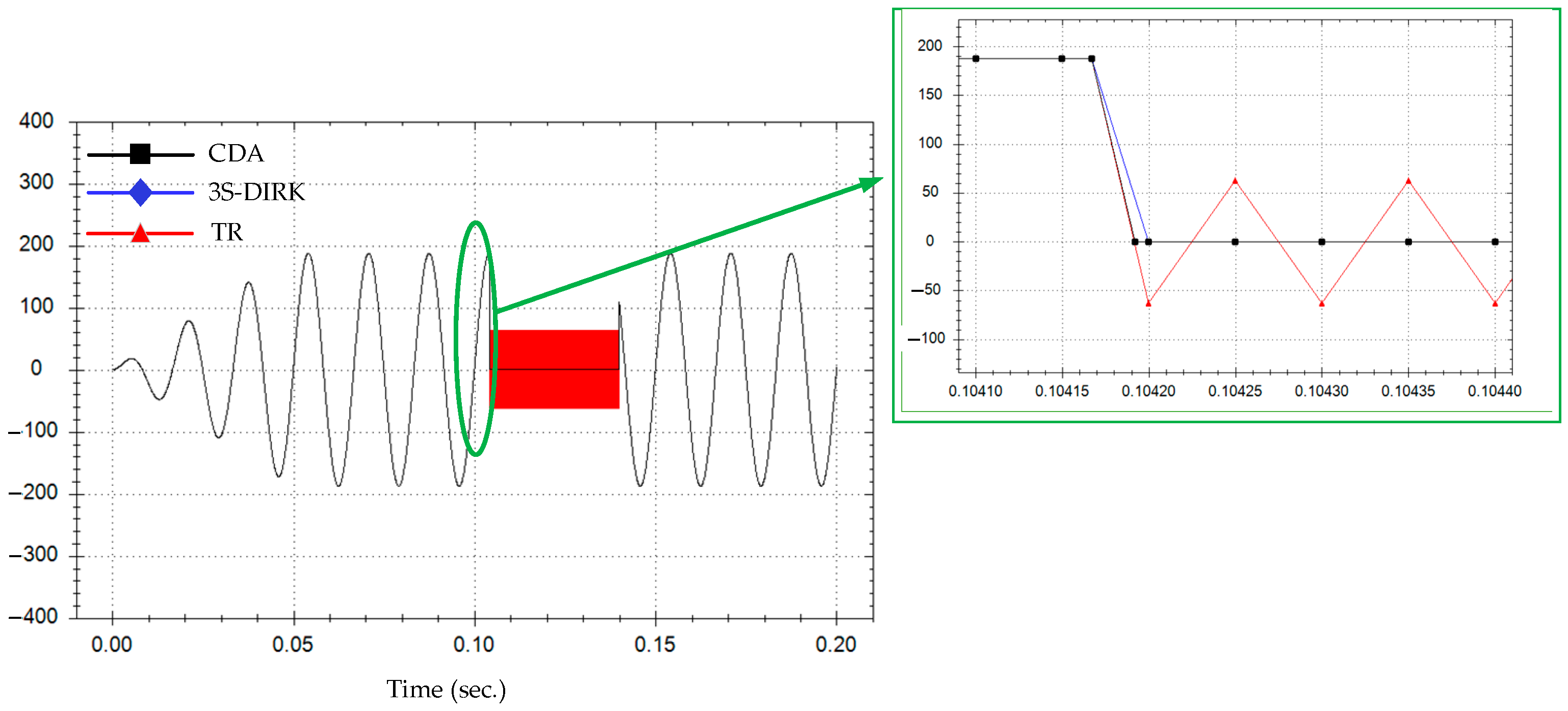
2.2. Linear Interpolation after TR Method
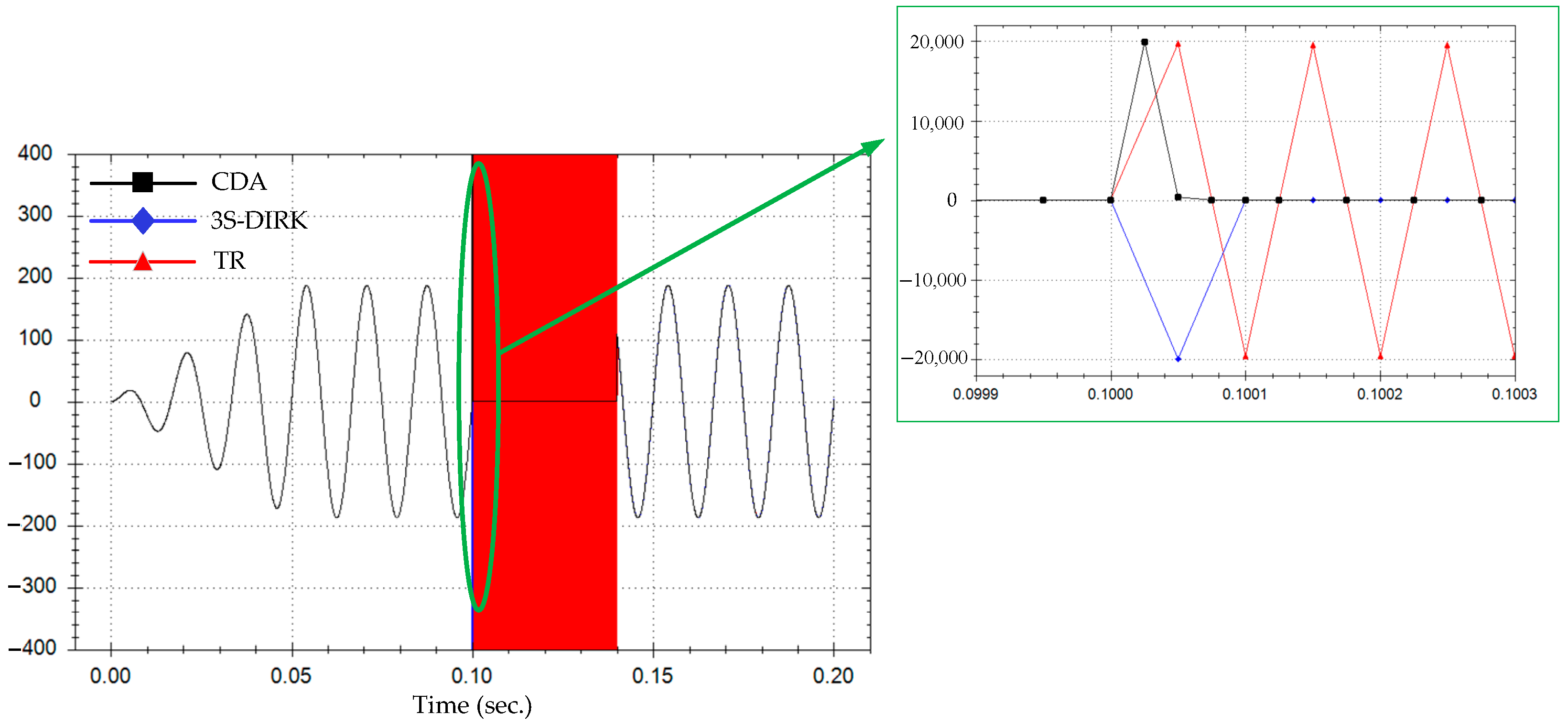
2.3. Linear Interpolation after BE Method
2.4. Error Analysis of CDA Scheme
3. 3S-DIRK-Based Integral Interpolation Scheme
3.1. 3S-DIRK
- Diagonally implicit RK formula (DIRK): This enables a separate computation for each stage, without the need to generate a large matrix, which has the advantage of being a multistep method.
- Singly diagonally implicit Runge–Kutta formula (SDIRK): The diagonal elements of the algorithm meeting this characteristic are identical, i.e., all the elements of are identical. When solving this special case of the DIRK algorithm, the Jacobi matrix is guaranteed to remain unchanged at each computational stage, which reduces the computational load of matrix decomposition.
- First-same-as-last formula (FSAL): In this formula, and , which means that the first stage of a step is the same as the last stage from the end of the previous step. This condition ensures that when solving rigid problems, order reduction will not occur in the algorithm [34].
3.2. TR-3S-DIRK in Interpolation Process
3.3. BE2-3S-DIRK in Synchronous Process
- The variable step size can be used for interpolation synchronization;
- The computational accuracy is improved to the second order, while the first-order error brought by the BE algorithm is corrected;
- It satisfies L-stability, which can eliminate the numerical oscillation in the computation.
4. Application of 3S-DIRK in EMT Program
4.1. Application of 3S-DIRK in DAEs
4.2. Linear Inductors
4.3. Linear Capacitors
5. Case Study
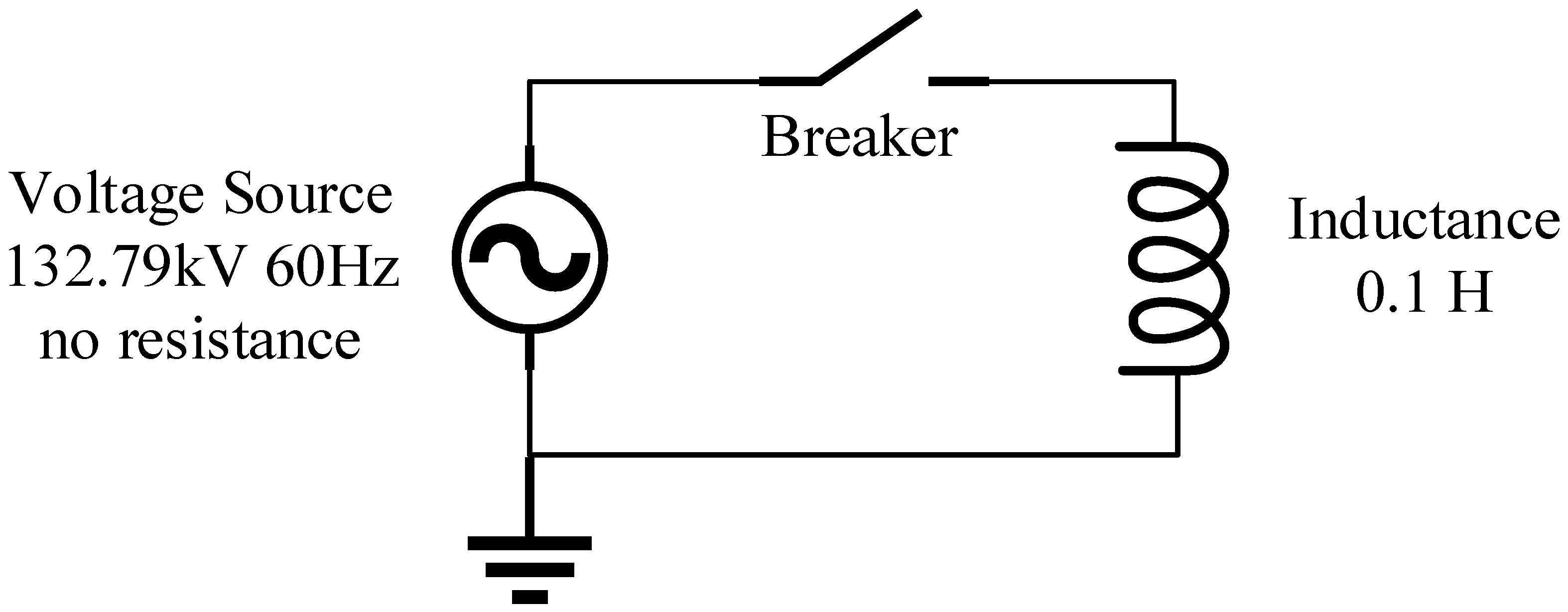
5.1. Case A: Series R-L Circuit
5.1.1. Case A1: Breaker of Half-Controlled Type
5.1.2. Case A2: Breaker of Full-Controlled Type
5.2. Case B: AC/DC Hybrid Power Systems
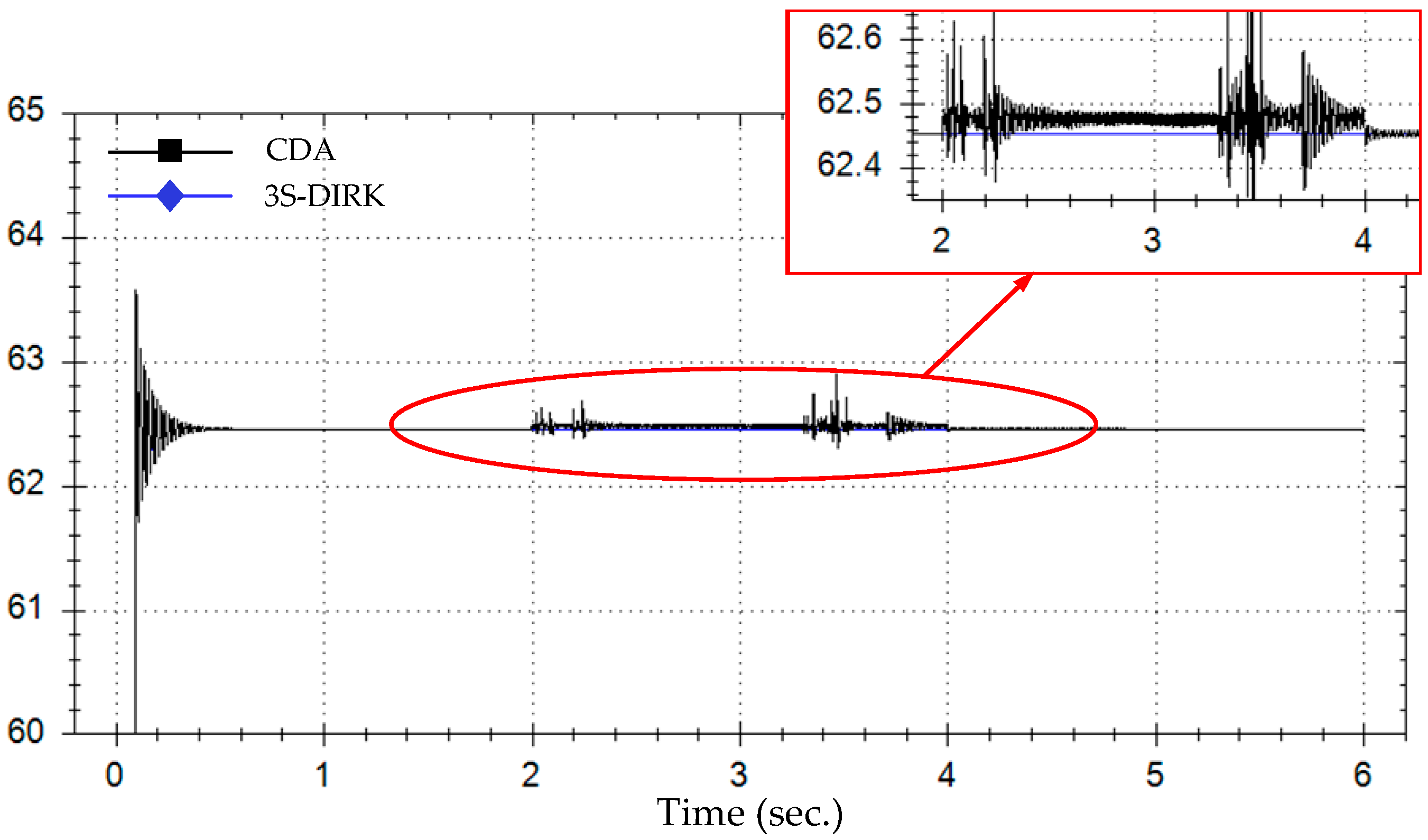
5.2.1. Case B1: Impact of the BE Algorithm
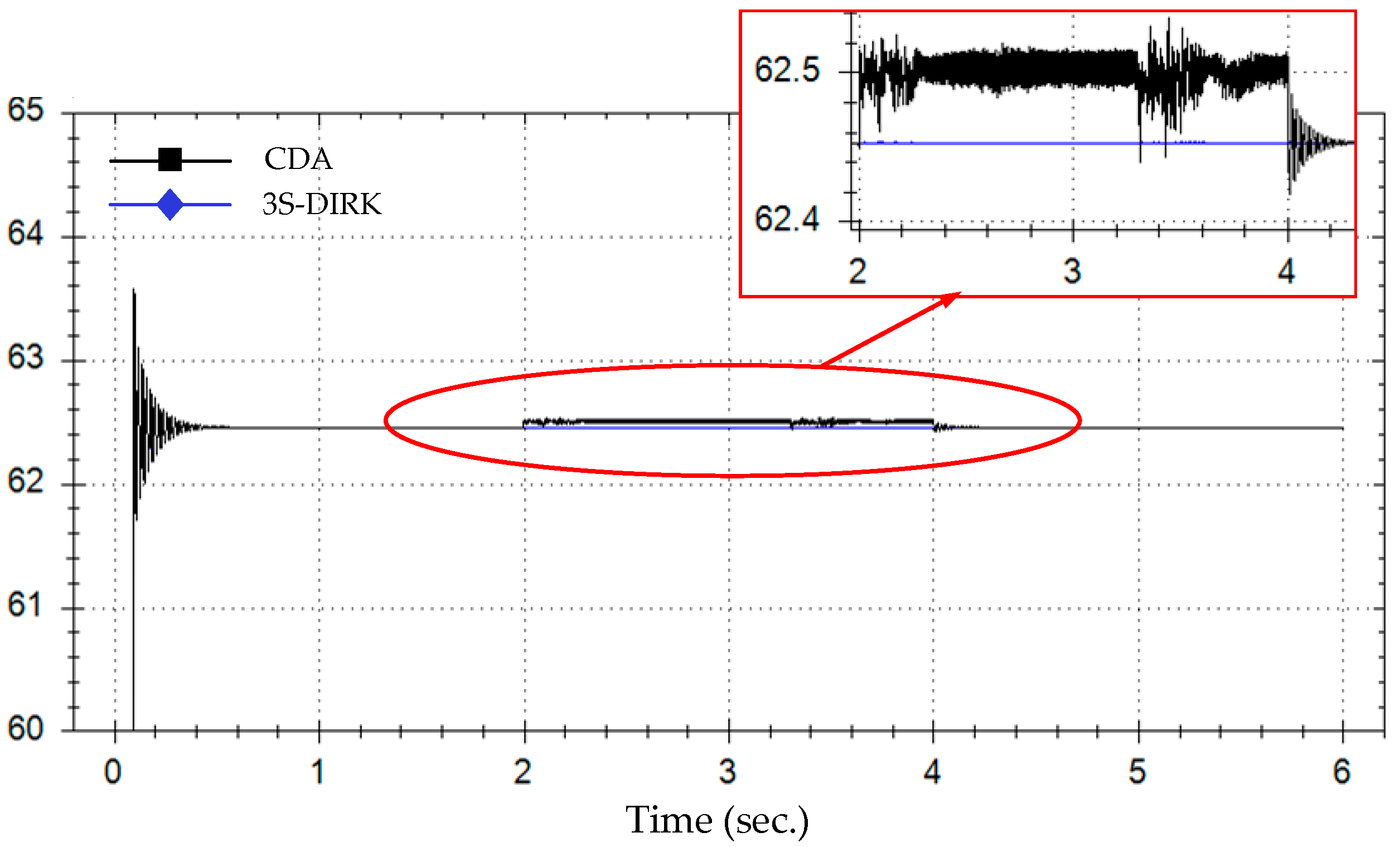
5.2.2. Case B2: Impact of Interpolation
5.2.3. Case B3: Impact of the Number of Computations Using the BE Algorithm
5.2.4. Case B4: Impact of the Simulation Step
6. Conclusions
Author Contributions
Funding
Data Availability Statement
Conflicts of Interest
Nomenclature
| Abbreviations | |
| EMT | Electromagnetic transient |
| RK | Runge–Kutta |
| DIRK | Diagonally implicit RK formula |
| SDIRK | Singly diagonally implicit Runge–Kutta formula |
| FSAL | First-same-as-last formula |
| 3S-DIRK | Three-stage diagonally implicit Runge–Kutta |
| 2S-DIRK | Two-stage diagonally implicit Runge–Kutta |
| TR | Trapezoidal rule |
| BE | Backward Euler |
| TR-3S-DIRK | Three-stage diagonally implicit Runge–Kutta methods combined with trapezoidal rule |
| BE2-3S-DIRK | Three-stage diagonally implicit Runge–Kutta methods combined with backward Euler twice |
| DAEs | Differential–algebraic equations |
| ODEs | Ordinary differential equations |
| TR-BDF2 | Trapezoidal method with the second-order backward difference formula |
| LCC-HVDC | Line-commutated converter-based high-voltage direct current |
| IGBT | Insulated-gate bipolar transistor |
| CDA | Critical damping adjustment |
| Variables | |
| f(t,y) | Function of the differential equation, representing the derivative of y with respect to t |
| tn, tn+1 | Time at the n-th and n+1-th time step as shown in Figure 1 |
| yn, yn+1 | Value at the n-th and n+1-th time step, respectively |
| kT, kB | Interpolation coefficients in Stage 1 and Stage 4 as in Figure 1 |
| h | Step size |
| New step size | |
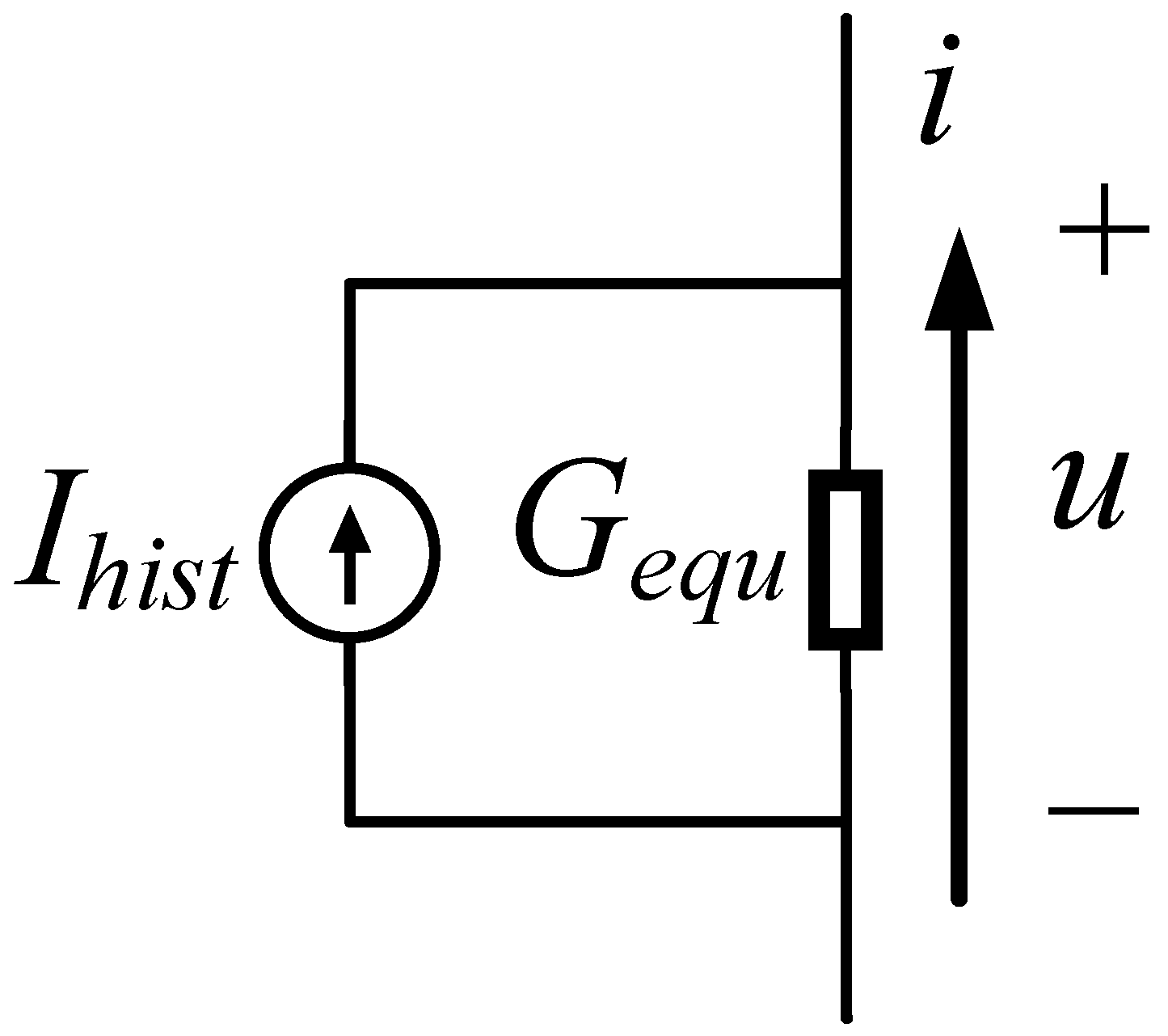
| Gequ | Equivalent admittance in equivalent circuit |
| Ihist | History current in equivalent circuit |
| u | Instantaneous voltage |
| i | Instantaneous current |
| L | Inductance of inductor |
| C | Capacitance of capacitor |
| Voltage phase angle | |
| Current phase angle | |
| R | Resistance |
| ω | Angular frequency |
| c, b | Vector of s size as in Equation (4) |
| A, C | Matrix of size s x s as in Equation (4) |
Appendix A. Error Calculations of BE Method and Interpolation Algorithm
Appendix A.1. Error in Single-Phase Inductor

| TR | BE | Interpolation (k = 0.5) | |
|---|---|---|---|
| Formula | |||
| Magnitude | |||
| Angle |
Appendix A.2. Error in Three-Phase Inductor
| TR | BE | Interpolation (k = 0.5) | |
|---|---|---|---|
| Formula | |||
| Active power | |||
| Reactive power |
Appendix A.3. Error in Three-Phase Capacitor
| TR | BE | Interpolation (k = 0.5) | |
|---|---|---|---|
| Formula | |||
| Active power | |||
| Reactive power |
Appendix B. Derivation Process of 3S-DIRK of Linear Inductor and Capacitor
Appendix B.1. Linear Inductor
Appendix B.2. Linear Capacitors
References
- Mahseredjian, J.; Dinavahi, V.; Martinez, J.A. Simulation tools for electromagnetic transients in power systems: Overview and challenges. IEEE Trans. Power Del. 2009, 24, 1657–1669. [Google Scholar] [CrossRef]
- Ming, Y.; Yongming, Z.; Ziqian, Z. Review of electromagnetic transient simulation algorithms for power system. Elect. Meas. Instrum. 2022, 59, 10–19. [Google Scholar]
- Tanaka, Y.; Baba, Y. Study of a numerical integration method using the compact scheme for electromagnetic transient simulations. Electr. Power Syst. Res. 2023, 223, 109666. [Google Scholar] [CrossRef]
- Subedi, S.; Rauniyar, M.; Ishaq, S.; Hansen, T.M.; Tonkoski, R.; Shirazi, M.; Wies, R.; Cicilio, P. Review of methods to accelerate electromagnetic transient simulation of power systems. IEEE Access 2021, 9, 89714–89731. [Google Scholar] [CrossRef]
- Gear, W. Simultaneous numerical solution of differential-algebraic equations. IEEE Trans. Circuit Theory 1971, 18, 89–95. [Google Scholar] [CrossRef]
- Butcher, J.C. Stability of implicity runge-kutta methods. In Numerical Methods for Ordinary Differential Equations, 2nd ed.; John Wiley & Sons Ltd.: New York, NY, USA, 2008; pp. 230–258. [Google Scholar]
- Tant, J.; Driesen, J. On the numerical accuracy of electromagnetic transient simulation with power electronics. IEEE Trans. Power Deliv. 2018, 33, 2492–2501. [Google Scholar] [CrossRef]
- Dommel, H.W. Digital computer solution of electromagnetic transients in single- and multiphase networks. IEEE Trans. Power Appar. Syst. 1969, 88, 734–741. [Google Scholar] [CrossRef]
- Pordanjani, S.R.; Mahseredjian, J.; Naïdjate, M.; Bracikowski, N.; Fratila, M.; Rezaei-Zare, A. Electromagnetic modeling of inductors in EMT-type software by three circuit-based methods. Electr. Power Syst. Res. 2022, 211, 108304. [Google Scholar] [CrossRef]
- Wen, H.C.; Ruehli, A.; Brennan, P. The modified nodal approach to network analysis. IEEE Trans. Circuits Syst. 1975, 22, 504–509. [Google Scholar]
- Ametani, A. Electromagnetic transients program: History and future. IEEJ Trans. Electr. Electron. Eng. 2021, 16, 1150–1158. [Google Scholar] [CrossRef]
- Marti, J.R.; Lin, J. Suppression of numerical oscillations in the EMTP. IEEE Power Eng. Rev. 1989, 9, 71–72. [Google Scholar] [CrossRef]
- Alvarado, F.L.; Lasseter, R.H.; Sanchez, J.J. Testing of trapezoidal integration with damping for the solution of power transient problems. IEEE Trans. Power Appar. Syst. 1983, 102, 3783–3790. [Google Scholar] [CrossRef]
- Noda, T.; Takenaka, K.; Inoue, T. Numerical integration by the 2-stage diagonally implicit Runge-Kutta method for electromagnetic transient simulations. IEEE Trans. Power Deliv. 2009, 24, 390–399. [Google Scholar] [CrossRef]
- Noda, T.; Kikuma, T.; Yonezawa, R. Supplementary techniques for 2S-DIRK-based EMT simulations. Electr. Power Syst. Res. 2014, 115, 87–93. [Google Scholar] [CrossRef]
- Olaniyan, A.S.; Bakre, O.F.; Akanbi, M.A. A 2-stage implicit Runge-Kutta method based on heronian mean for solving ordinary differential equations. Pure Appl. Math. J. 2020, 9, 84–90. [Google Scholar] [CrossRef]
- Watson, N.R.; Irwin, G.D. Comparison of root-matching techniques for electromagnetic transient simulation. IEEE Trans. Power Deliv. 2000, 15, 629–634. [Google Scholar] [CrossRef]
- Ye, J.; Xie, J.; Wang, Y.; Zhang, L.; Li, B.; Lv, J.; Li, K.; Jin, S.; Xu, Y.; Ma, W. Electromagnetic transient simulation algorithm for nonlinear elements based on rosenbrock numerical integration method. IEEE Access 2024, 12, 66981–66992. [Google Scholar] [CrossRef]
- Cibik, A.; Eroglu, F.G.; Kaya, S. Analysis of second order time filtered backward Euler method for MHD equations. J. Sci. Comput. 2020, 82, 38. [Google Scholar] [CrossRef]
- Lin, J.; Marti, J.R. Implementation of the CDA procedure in the EMTP. IEEE Trans. Power Systems 1990, 5, 394–402. [Google Scholar]
- Kui, W.; Ying, S. Modeling and simulation of nonlinear component algorithm. Power Syst. Clean Energy 2010, 26, 34–37. [Google Scholar]
- Zou, M.; Mahseredjian, J.; Delourme, B.; Joos, G. On interpolation and reinitialization in the simulation of transients in power electronic systems. In Proceedings of the 14th Power Systems Computation Conference (PSCC 2002), Sevilla, Spain, 24–28 June 2002. [Google Scholar]
- Kuffel, P.; Kent, K.; Irwin, G. The implementation and effectiveness of linear interpolation within digital simulation. Int. J. Electr. Power Energy Syst. 1997, 19, 221–227. [Google Scholar] [CrossRef]
- Strunz, K.; Linares, L.; Marti, J.R.; Huet, O.; Lombard, X. Efficient and accurate representation of asynchronous network structure changing phenomena in digital real time simulators. IEEE Trans. Power Syst. 2000, 15, 586–592. [Google Scholar] [CrossRef]
- Strunz, K. Flexible numerical integration for efficient representation of switching in real time electromagnetic transients simulation. IEEE Trans. Power Deliv. 2004, 19, 1276–1283. [Google Scholar] [CrossRef]
- Nzale, W.; Mahseredjian, J.; Fu, X.; Kocar, I.; Dufour, C. Improving Numerical Accuracy in Time-Domain Simulation for Power Electronics Circuits. IEEE Open Access J. Power Energy 2021, 8, 157–165. [Google Scholar] [CrossRef]
- Li, P.; Meng, Z.; Fu, X.; Yu, H.; Wang, C. Interpolation for power electronic circuit simulation revisited with matrix exponential and dense outputs. Electr. Power Syst. Res. 2020, 189, 106714. [Google Scholar] [CrossRef]
- Wang, C.; Fu, X.; Li, P.; Wu, J.; Wang, L. Multiscale Simulation of Power System Transients Based on the Matrix Exponential Function. IEEE Trans. Power Syst. 2017, 32, 1913–1926. [Google Scholar] [CrossRef]
- Kennedy, C.A.; Carpenter, M.H. Diagonally Implicit Runge-Kutta Methods for Ordinary Differential Equations. A Review; National Aeronautics and Space Administration: Washington, DC, USA, 2016. [Google Scholar]
- Kennedy, C.A.; Carpenter, M.H. Diagonally implicit Runge–Kutta methods for stiff ODEs. Appl. Numer. Math. 2019, 146, 221–244. [Google Scholar] [CrossRef]
- da Silva, C.C.; Lessig, C. Variational symplectic diagonally implicit Runge-Kutta methods for isospectral systems. BIT Numer. Math. 2022, 62, 1823–1840. [Google Scholar] [CrossRef]
- Kamiński, M.; Corigliano, A. Numerical solution of the Duffing equation with random coefficients. Meccanica 2015, 50, 1841–1853. [Google Scholar] [CrossRef]
- Butcher, J.C. Coefficients for the study of Runge-Kutta integration processes. J. Aust. Math. Soc. 1963, 3, 185–201. [Google Scholar] [CrossRef]
- Prothero, A. Robinson, Stability and accuracy of one-step methods for solving stiff systems of ordinary differential equations. Math. Comp. 1974, 28, 145–162. [Google Scholar] [CrossRef]
- Oni, O.E.; Davidson, I.E.; Mbangula, K.N. A review of LCC-HVDC and VSC-HVDC technologies and applications. In Proceedings of the 2016 IEEE 16th International Conference on Environment and Electrical Engineering (EEEIC), Florence, Italy, 7–10 June 2016; IEEE: New York City, NY, USA, 2016; pp. 1–7. [Google Scholar]

| Error (MW) | CDA | 3S-DIRK |
|---|---|---|
| Case B1 | 0.0404 | 0.0002 |
| Case B2 | 0.4454 | 0.0003 |
| Case B3 | 0.0831 | 0.0005 |
| Case B4 | 0.1454 | 0.0032 |
Disclaimer/Publisher’s Note: The statements, opinions and data contained in all publications are solely those of the individual author(s) and contributor(s) and not of MDPI and/or the editor(s). MDPI and/or the editor(s) disclaim responsibility for any injury to people or property resulting from any ideas, methods, instructions or products referred to in the content. |
© 2024 by the authors. Licensee MDPI, Basel, Switzerland. This article is an open access article distributed under the terms and conditions of the Creative Commons Attribution (CC BY) license (https://creativecommons.org/licenses/by/4.0/).
Share and Cite
Sun, K.; Chen, K.; Cen, H.; Tan, F.; Ye, X. Study of a Numerical Integral Interpolation Method for Electromagnetic Transient Simulations. Energies 2024, 17, 3837. https://doi.org/10.3390/en17153837
Sun K, Chen K, Cen H, Tan F, Ye X. Study of a Numerical Integral Interpolation Method for Electromagnetic Transient Simulations. Energies. 2024; 17(15):3837. https://doi.org/10.3390/en17153837
Chicago/Turabian StyleSun, Kaiyuan, Kun Chen, Haifeng Cen, Fucheng Tan, and Xiaohui Ye. 2024. "Study of a Numerical Integral Interpolation Method for Electromagnetic Transient Simulations" Energies 17, no. 15: 3837. https://doi.org/10.3390/en17153837