An Improved MGM (1, n) Model for Predicting Urban Electricity Consumption

Abstract

The MGM (1, n) model has the characteristics of less data required, simple modeling, and high prediction accuracy. It has been successfully applied to short-term forecasting across various economic, social, and technological domains, yielding promising outcomes. There is insufficient attention paid to the interpolation coefficient of the model. The interpolation coefficients determine the extent of model fitting, which, in turn, impacts its prediction accuracy. This study made some improvements to the interpolation coefficients and proposed an improved MGM (1, n) model. IMGM (1, n) model and MGM (1, n) model were employed to compare the performance of the improved MGM (1, n) model. Upon a series of comparisons and analyses, it was concluded that the improved MGM (1, n) model has higher fitting and prediction accuracy than the other two forecasting methods. The method was used to forecast the short-term electricity consumption of Linfen City. The findings revealed that by 2030, the electricity demand in Linfen City is projected to be 563.7 billion kWh.

1. Introduction

Energy security is a guarantee of the normal operation of the urban economy and society. As the economy undergoes transformation and gradual implementation of China’s carbon emission policy, the proportion of electricity demand in the urban energy structure is set to increase. Linfen City is located in the southern part of Shanxi Province, China. The city’s economic development is excessively reliant on resource-intensive industries such as the coal industry and the steel industry. The massive consumption of coal has resulted in severe air pollution and excessive CO₂ emissions. To protect the environment and promote sustainable economic development, during the 13th five-year plan period, Shanxi Province has committed to no further expansion of coal-fired power capacity. The growing power demand poses a huge challenge to the safe operation and power supply. Under these challenging circumstances, ensuring both power security and a transition to new economic growth models poses a formidable task for Linfen City. Furthermore, the construction of an urban power system requires a significant amount of time and is highly capital-intensive. Therefore, conducting scientific power demand analysis and forecasting offers practical guidance for the development of urban energy systems.

Electricity demand forecasting is a crucial element in power planning. If the forecasted demand is less than the actual demand, it will result in reduced power supply and power outages. Conversely, if the forecasted demand exceeds the actual demand, it will result in power waste. Given the numerous urban electricity users and the extensive data they produce, collecting electricity usage data from different departments is challenging. This makes urban electricity demand forecasting particularly complex. As a significant area in power systems, energy consumption has been attracting considerable research in recent decades. The literature on electricity demand could be classified into two aspects. The first is electricity demand models. The forecasting models include neural network models, intelligent data mining models, regression models, hybrid prediction models, grey forecasting models, and so on. Neural network models and intelligent data mining models require the quantification of large amounts of historical data to establish predictive models. These models have significant advantages in processing large amounts of nonlinear data and predicting the energy demand of complex systems [1,2,3,4,5]. The regression model takes electricity demand as the independent variable, and its influencing factors as the dependent variable. It establishes a linear function between electricity demand and influencing factors to predict the total electricity demand [6,7,8,9]. The grey prediction model is a mathematical model that predicts electricity demand or supply based on a small amount of data [10,11,12,13,14,15]. The hybrid prediction model integrates the strengths of various prediction models, offering high prediction accuracy for energy demand [16,17,18]. The second is the influencing factors of electricity demand. The factors that affect electricity demand include economic development level, population size, per capita GDP, industrial structure, technological level, urbanization level, industrialization level, and so on. Tapio decoupling model, wavelet analysis, regression analysis, and so on are the main analysis methods [7,19,20]. In addition, as the logarithmic mean Divisia index (LMDI) method has better performance in theoretical basis, operability, and result presentation, it is widely applied to analyze the impact of various factors on electricity demand in different regions [21,22,23,24].

In light of the above literature, energy consumption is one of the vital energy security problems that requires quantitative analysis of its influencing factors and development trends. To forecast energy consumption, an improved MGM (1, n) model is proposed. The multivariate grey prediction model, commonly referred to as MGM (1, n), is specifically designed to tackle data prediction challenges within incomplete information systems. The model employs accumulation techniques to formulate a differential equation, which, combined with methodologies like the least squares method and time response functions, effectively uncovers inherent patterns within multivariable time series. This, in turn, enables precise predictions of future trends. The numeral “1” in the model signifies the presence of a single differential equation, while “n” denotes the inclusion of n variables, making it well-suited for addressing time series prediction problems influenced by multiple factors [25]. During the last several decades, many types of research have been conducted on the MGM (1, n) model trying to improve the precision of forecasting. Wang presents the multivariable non-equidistance method to forecast the teenage growth level in China [26]. Based on the patterns of first-order generated sequences, Xiong et al. developed an IMGM (1, n) model that exhibits superior prediction accuracy by employing exponential functions to reconstruct the background values of MGM (1, n) [27]. Chen et al. apply a nonlinear optimization model in the bottomless foundation pit supporting structure [28]. Xiong et al. found that the non-homogeneous exponential method could fit the accumulated sequences of the MGM (1, n) model [29]. Wu and Zhang adjusted the weight of the data to improve the fitting and prediction accuracy of the accumulated sequences of the MGM (1, n) model [30]. Ma et al. integrated the MGM (1, n) model with kernel techniques to develop a predictive model for complex nonlinear time series [31]. Zeng improved the prediction accuracy of the MGM (1, n) model by reconstructing background values [32]. However, for the MGM (1, n) model, the background value is calculated in terms of the interpolation coefficient γ = 0.5. It is inaccurate when the interpolation coefficient is set as a constant. Few studies have researched the interpolation coefficient to improve the predictive precision of the model. This article combines the particle swarm optimization and fitness function to optimize the interpolation coefficients of the model, thereby improving the prediction and fitting accuracy of the model. The results show that the improved MGM (1, n) model has a higher fitting and prediction accuracy than the IMGM (1, n) model and the MGM (1, n) model. The improved MGM (1, n) is employed to forecast the electricity consumption of Linfen City and the LMDI method is applied to analyze the impact of different factors on energy consumption.

2. Data and Methods

2.1. Data Source

This article collected annual data on gross domestic production, the secondary sector, primary and tertiary industries, permanent residents, and electricity consumption in different industries, for 2010–2022 from the Linfen City Statistical Yearbook and Linfen City Statistical Bulletin.

2.2. Logarithmic Mean Divisia Index (LMDI) Method

2.2.1. The Index Decomposition Method

Yoichi Kaya proposed the Kaya model at the IPCC seminar in 1989, and the LMDI method was developed based on the IDE model. The model is widely used in research on environmental and energy issues.

In this paper, the method is shown in Equations (1)–(7).

$$E=E_d+E_r$$

(1)

$$E_d={\sum }_{i=1}^3{E}_i={\sum }_{i=1}^3{\displaystyle \frac{E_i}{G_i}}\times {\displaystyle \frac{G_i}{G}}\times G$$

(2)

$$E_d={\sum }_{i=1}^3{T}_i\times S_i\times G$$

(3)

$$E_r={\displaystyle \frac{E_r}{G}}\times {\displaystyle \frac{G}{P}}\times P$$

(4)

$$E_r=Q\times I\times P$$

(5)

$$E_d^t-E_d^0={\sum }_{i=1}^3{T}_i^t\times S_i^t\times G^t-{\sum }_{i=1}^3{T}_i^0\times S_i^0\times G^0=∆E_T+∆E_S+∆E_G$$

(6)

$$E_r^t-E_r^0=Q^t\times I^t\times P^t-Q^0\times I^0\times P^0=∆E_Q+∆E_I+∆E_P$$

(7)

This paper studies the electricity consumption of Linfen City. $E$ represents the total electricity demand; $E_d$ and $E_r$ represent industrial and residential electricity consumption, respectively; $E_i$ represents the electricity demand of different industries; $G$ represents the gross domestic product of Lingfen City; $G_i$ represents the output value of different industries; and $P$ is the number of resident populations at the end of the year in Linfen City. Among the factors affecting power consumption, $T_i$ is the electricity demand per unit output value of different industries, representing the technological level, and $S_i$ is the industrial structure. $G$ is the economic scale effect, $Q$ is the electricity consumption per unit output value, $I$ represent the regional per capita gross domestic product (GNP), and $P$ represents the population scale effect. $∆E_T$, $∆E_S$, $∆E_G$, $∆E_Q$, $∆E_I$, and $∆E_P$ represent the contribution value of different influencing factors on electricity consumption.

2.2.2. The Improved MGM (1, n) Model

MGM (1, n) is derived from the GM (1, 1) model, but it is not a linear combination of the GM (1, 1) model. It is a multivariable grey forecasting model. For the MGM (1, n) model, the interpolation coefficient γ = shengbei0.5 reduces the fitting accuracy of the model, resulting in low prediction accuracy. Therefore, it is necessary to optimize the interpolation coefficient to improve the fitting accuracy and prediction accuracy of the model. In this paper, $n$ parameters were inserted into the MGM (1, n) model to optimize the interpolation coefficient of this model. Furthermore, this paper combines the particle swarm optimization algorithm and fitness function to solve $n$ parameters. Figure 1 shows the methodological diagram of the MGM (1, n) model. The procedures of the improved MGM (1, n) could be deduced as follows.

Given the initial multivariate time series $X^0$, which is shown in Equation (8)

$$X^0=\left\{X_1^{\left(0\right)},X_2^{\left(0\right)},\dots ,X_n^{\left(0\right)}\right\}$$

(8)

where $X_k^{\left(0\right)}=\left\{x_k^{\left(0\right)}\left(1\right),x_k^{\left(0\right)}\left(2\right),\dots ,x_k^{\left(0\right)}\left(m\right)\right\}$, $x_k^{\left(0\right)}\left(i\right)$ is the $i$th value of $X_j^{\left(0\right)}$, $k=1,2,\dots ,n$.

The first-order cumulative value of different indicators is shown in Equation (9)

$$X^{\left(1\right)}=\left\{X_1^{\left(1\right)},X_2^{\left(1\right)},\dots ,X_n^{\left(1\right)}\right\}$$

(9)

where $X_k^{\left(1\right)}=\left\{x_k^{\left(1\right)}\left(1\right),x_k^{\left(1\right)}\left(2\right),\dots ,x_k^{\left(1\right)}\left(m\right)\right\}$, $x_k^{\left(1\right)}\left(i\right)=\sum _{j=1}^i{x}_k^{\left(0\right)}\left(j\right)$, $i=1,2,\dots ,m$, $k=\mathrm{1,2},\dots ,n$.

The generated sequence of $X^{\left(1\right)}$ is shown in Equation (10)

$$Z_k^{\left(1\right)}=\left\{z_k^{\left(1\right)}\left(2\right),z_k^{\left(1\right)}\left(3\right),\dots ,z_k^{\left(1\right)}\left(m\right)\right\}$$

(10)

in which, $z_k^{\left(1\right)}\left(j\right)={\displaystyle \frac{1}{2}}{x}_k^{\left(1\right)}\left(j\right)+{(1-{\displaystyle \frac{1}{2}})x}_k^{\left(1\right)}\left(j-1\right),j=2,3,\dots ,m$.

The MGM (1, n) model could be written as Equation (11)

$${\displaystyle \frac{d{X}^{\left(1\right)}\left(t\right)}{dt}}=A{X}^{\left(1\right)}\left(t\right)+B$$

(11)

where $A={\left(a_{ij}\right)}_{n\times n}$, ${B=(b_1,b_2,\dots ,b_n)}^T$, $X^{\left(1\right)}\left(k\right)={\left\{x_1^{\left(1\right)}\left(k\right),x_2^{\left(1\right)}\left(k\right),\dots ,x_n^{\left(1\right)}\left(k\right)\right\}}^T$.

The discretization of Equation (11) is shown in Equation (12)

$$\begin{gathered} x_j^0\left(k\right)={\sum }_{l=1}^n{a}_{jl}{z}_l^{\left(1\right)}\left(k\right)+b_j \\ j=\mathrm{1,2},\dots ,n, k=\mathrm{2,3},\dots ,m \end{gathered}$$

(12)

in which, $A$ and $B$ are parameter matrices to be estimated. The solution of parameters in Equation (12) is shown in Equation (13)

$$\left({\widehat{a}}_1,{\widehat{a}}_2,\dots ,{\widehat{a}}_n\right)={\left(P^{T}P\right)}^{-1}{P}^T\left(Q_1,Q_2,\dots ,Q_n\right)$$

(13)

where ${\widehat{a}}_i={\left\{{\widehat{a}}_{i1},{\widehat{a}}_{i2},\dots ,{\widehat{a}}_{in},{\widehat{b}}_i\right\}}^T$, $Q_i={\left\{x_i^{\left(0\right)}\left(2\right),x_i^{\left(0\right)}\left(3\right),\dots ,x_i^{\left(0\right)}\left(m\right)\right\}}^T$,$i=\mathrm{1,2},\dots ,n$. $A={\left({\widehat{a}}_{ij}\right)}_{n\times n}$, $\mathrm{B}=({\widehat{b}}_1,{\widehat{b}}_2,\dots ,{\widehat{b}}_n)$ and

$$P=\left[\begin{array}{ccc}\begin{array}{cc}{z}_1^{\left(1\right)}\left(2\right)& z_2^{\left(1\right)}\left(2\right)\end{array}& \dots & \begin{array}{cc}{z}_n^{\left(1\right)}\left(2\right)& 1\end{array}\\ \begin{array}{cc}{z}_1^{\left(1\right)}\left(3\right)& z_2^{\left(1\right)}\left(3\right)\end{array}& \dots & \begin{array}{cc}{z}_n^{\left(1\right)}\left(3\right)& 1\end{array}\\ \begin{array}{cc}\begin{array}{c}⋮\\ z_1^{\left(1\right)}\left(m\right)\end{array}& \begin{array}{c}⋮\\ z_2^{\left(1\right)}\left(m\right)\end{array}\end{array}& \begin{array}{c}\ddots \\ \dots \end{array}& \begin{array}{c}\begin{array}{cc}⋮& ⋮\end{array}\\ \begin{array}{cc}{z}_n^{\left(1\right)}\left(m\right)& 1\end{array}\end{array}\end{array}\right].$$

The response sequence of Equation (11) is shown in Equation (14)

$${\widehat{X}}^{\left(1\right)}\left(k\right)=e^{A\left(k-1\right)}\left(X^{\left(1\right)}\left(1\right)+A^{-1}B\right)-A^{-1}B$$

(14)

The predicted values based on the original data sequence can be obtained by performing a decrement operation on Equation (14), which is shown in Equation (15)

$${\widehat{X}}^{\left(0\right)}\left(k\right)={\widehat{X}}^{\left(1\right)}\left(k\right)-{\widehat{X}}^{\left(1\right)}\left(k-1\right)$$

(15)

where $k=\mathrm{2,3},\dots ,m$, ${\widehat{X}}^{\left(0\right)}\left(k\right)=\left\{{\widehat{x}}_k^{\left(0\right)}\left(1\right),{\widehat{x}}_k^{\left(0\right)}\left(2\right),\dots ,{\widehat{x}}_k^{\left(0\right)}\left(n\right)\right\}$.

For the MGM (1, n) model, it is inaccurate to solve the background value $z_k^{\left(1\right)}\left(j\right), j=2, 3, \dots , m$. To optimize the model, the grey variable $\widehat{P}$ will supersede the values $P$ to estimate the grey differential parameter matrix $A$ and $B$, which is shown in Equation (16).

$$\widehat{P}=P=\left[\begin{array}{ccc}\begin{array}{cc}{\widehat{z}}_1^{\left(1\right)}\left(2\right)& {\widehat{z}}_2^{\left(1\right)}\left(2\right)\end{array}& \dots & \begin{array}{cc}{\widehat{z}}_n^{\left(1\right)}\left(2\right)& 1\end{array}\\ \begin{array}{cc}{\widehat{z}}_1^{\left(1\right)}\left(3\right)& {\widehat{z}}_2^{\left(1\right)}\left(3\right)\end{array}& \dots & \begin{array}{cc}{\widehat{z}}_n^{\left(1\right)}\left(3\right)& 1\end{array}\\ \begin{array}{cc}\begin{array}{c}⋮\\ {\widehat{z}}_1^{\left(1\right)}\left(m\right)\end{array}& \begin{array}{c}⋮\\ {\widehat{z}}_2^{\left(1\right)}\left(m\right)\end{array}\end{array}& \begin{array}{c}\ddots \\ \dots \end{array}& \begin{array}{c}\begin{array}{cc}⋮& ⋮\end{array}\\ \begin{array}{cc}{\widehat{z}}_n^{\left(1\right)}\left(m\right)& 1\end{array}\end{array}\end{array}\right]$$

(16)

${\widehat{z}}_i^{\left(1\right)}\left(j\right)={\lambda }_i{x}_i^{\left(1\right)}\left(j\right)+{(1-{\lambda }_i)x}_i^{\left(1\right)}\left(j-1\right)$, $i=\mathrm{1,2},\dots ,n.j=\mathrm{2,3},\dots ,m$.

If ${\lambda }_i=1/2,(i=1, 2,\dots ,n)$, the improved model is degenerate to the MGM (1, n) model. Particle swarm optimization was adopted to search for the optimal solutions of the interpolation coefficient ${\lambda }_{i }(i=\mathrm{1,2}, \dots ,n)$ in the model, and then, the parameter matrix $A$ and $B$ was calculated.

2.2.3. Assessment of the Improved MGM (1, n) Model Forecasting Precision

The paper uses mean absolute percentage error (MAPE) to measure the prediction accuracy of the improved MGM (1, n) model [26,27,28]. Generally, the lower MAPE means better fitness between prediction values and actual values. The fitness function of the improved MGM (1, n) model is shown in Equation (17).

$$\mathrm{M}\mathrm{A}\mathrm{P}\mathrm{E}={\displaystyle \frac{1}{k}}{\sum }_{i=1}^k{\displaystyle \frac{\left|{\widehat{x}}_i^{\left(0\right)}-x_i^{\left(0\right)}\right|}{x_i^{\left(0\right)}}}\times 100\mathrm{\%}$$

(17)

where ${\widehat{x}}_i^{\left(0\right)}$ and $x_i^{\left(0\right)}$ are the fitting value and actual value, respectively, and $k$ is the number of time series.

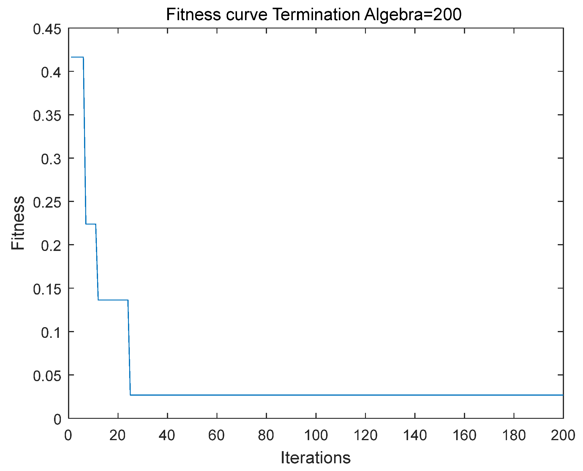
2.2.4. Particle Swarm Optimization

Kennedy and Eberhart inspired the foraging behavior patterns of birds and proposed the particle swarm optimization (PSO) algorithm [33]. Compared with other algorithms, the PSO algorithm is simple to program and has a fast convergence speed and advantages in solving dispersion problems. Therefore, this article used the PSO to calculate interpolation coefficients.

The velocity and particle iteration in this paper are defined as Equations (18) and (19).

$$v_{ij}^{k+1}=\omega v_{ij}^k+c_1{r}_1(p_{ij}^k-x_{ij}^k)+c_2{r}_2(g_{ij}^k-x_{ij}^k)$$

(18)

$$x_{ij}^{k+1}=x_{ij}^k+v_{ij}^k, (j=\mathrm{1,2},\cdots ,40)$$

(19)

The inertia weight $\omega$ is 1; $c_1$ and $c_2$ are acceleration factors; $r_1\in [0, 1]$ and $r_2\in [0, 1]$ are random numbers.

2.2.5. Validation of the Improved MGM (1, n) Model

Xiong et al. proved that IMGM (1, n) model had better performance than the MGM (1, n) model. To compare the advantage of the improved MGM (1, n) model, the data sequences $\mathrm{A}=\{8.64, 11.42, 13.54, 16.04, 19.02, 22.55, 26.72, 31.67, 37.55\}$ (Data sequence A) and $\mathrm{B}=\{9.66, 16.53, 18.64, 21.02, 23.69, 26.72, 30.12, 33.97, 38.29\}$ (Data sequence B) [27] were chosen as examples. For these data sequences, the first seven data were used for in-sample data to evaluate the simulation precision, while the other data would be used as out-of-date to evaluate the prediction performance. Here, the number of iterations and the population size are 200 and 20, respectively. The inertia weight $\omega$ is 1; the values of acceleration data are 0.9 and 0.9, respectively. Figure 2 shows the fitness cure of the improved MGM (1, 2). The results show that when the number of iterations reaches 20, the fitness function reaches its minimum value and the iteration stops. The IMGM (1, n) model and MGM (1, n) model were employed to compare the effectiveness of the improved MGM (1, n) model. The MAPEs and root-mean-square errors (RMSE) for in-sample and out-sample of these models for data sequences A and B are compared in

Table 1. The simulation precision of different models.

k	MGM (1, 2)		IMGM (1, 2)		Improved MGM (1, 2)
(1–7)	A	B	A	B	A	B
MAPE (%)	0.284	0.163	0.044	0.078	0.020	0.018

,

Table 2. Actual and forecasting values of MGM (1, 2), IMGM (1, 2), and improved MGM (1, 2) models.

k	Actual Value		MGM (1, 2)		IMGM (1, 2)		Improved MGM (1, 2)
8	31.67	33.97	31.54	33.86	31.66	33.99	31.67	33.95
9	37.55	38.29	37.36	38.17	37.52	38.38	37.53	38.27

and

Table 3. The prediction accuracy of different models.

k	MGM (1, 2)		IMGM (1, 2)		Improved MGM (1, 2)
8	0.411	0.324	0.032	0.059	0.012	0.060
9	0.506	0.313	0.080	0.235	0.049	0.046
MAPE (%)	0.459	0.319	0.056	0.147	0.031	0.053
RMSE	0.2055	0.1151	0.736	0.0652	0.0652	0.02

.

Table 1 reveals that the MAPEs of the IMGM (1, 2) model are 0.056% and 0.147, while the MAPEs of the improved MGM (1, 2) model for data sequences A and B are 0.02% and 0.018%, respectively. The results show that the improved MGM (1, 2) has a better fitting precision than the IMGM (1, 2) model and MGM (1, 2) model.

Table 3 shows the out-of-sample MAPEs. Per Table 2, the MAPEs of the IMGM (1, 2) model are 0.056% and 0.147% for data sequences A and B, respectively. The MAPEs of improved MGM (1, 2) models are 0.031% and 0.053% for data sequences A and B, respectively. Table 3 shows that the root-mean-square errors (RMSE) for the IMGM (1, 2) model and for the improved MGM (1, 2) models are 0.0652 and 0.02 for data sequences A and B, respectively. The values are all smaller than those of the MGM (1, 2) model and IMGM (1, 2) model. A variance test for the predicted values of datasets A and B indicates a value close to 0. The results indicate that the MAPEs for the improved MGM (1, 2) model were lower than for the IMGM (1, 2) and MGM (1, 2) models. This means that optimizing the interpolation parameters ${\lambda }_i (i=\mathrm{1,2})$ can optimize the fitting and prediction accuracy of the model. From the characteristics of these two indicators, the MGM model is suitable for predicting situations where multiple indicator variables are monotonically increasing but not suitable for situations where multiple indicator variables are fluctuating.

3. Empirical Results and Discussion

This article uses the LMDI method and the improved MGM (1, n) model to analyze and predict the power demand in Linfen City. The data from 2010 to 2022 were used to establish the forecasting model.

3.1. The Driving Factors of Electricity Demand in Linfen City

3.1.1. The Driving Factors of Industrial Electricity Consumption

Table 4. The influencing factors of industrial electricity demand in Linfen City from 2010 to 2022.

Year	$∆{\mathit{E}}_{\mathit{d}}$	$∆{\mathit{E}}_{\mathit{T}}$	$∆{\mathit{E}}_{\mathit{S}}$	$∆{\mathit{E}}_{\mathit{G}}$
2011	53,199.74	−132,894	43,317.66	142,775.7
2012	258,306.5	−27,275.4	33,601.71	251,980.1
2013	402,640.2	66,553.8	−17,913.8	354,000.2
2014	515,845.8	98,037.6	−65,516.7	483,324.8
2015	369,863.1	97,469.4	−12,5161	397,554.5
2016	423,062.3	118,228.1	−15,6176	461,010.7
2017	256,254.5	−35,982.1	−15,6070	448,307.2
2018	318,246.8	60,838.6	−19,4715	452,123.7
2019	506,871.5	112,777.7	−21,6961	611,054.5
2020	845,671.5	192,952.4	−23,6792	889,511.4
2021	1,083,334	−246,456	−65,114.9	1,394,905
2022	968,506.8	−586,773	64,350.83	1,490,928

shows the decomposition of the effects of factors influencing industrial electricity demand in Linfen City from 2010 to 2022. Overall, the demand for industrial electricity in Linfen City has shown a growing trend over the past 12 years. Among them, the economic scale effect dominates the impact on electricity consumption and shows a positive effect. Technological innovation and industrial restructuring have a restraining effect on electricity consumption. This indicates that technological progress and industrial restructuring can improve electricity efficiency. Due to the excessive dependence on heavy industry in Linfen City, the slow transformation, and upgrading of industries, as well as the lack of technological innovation, the impact of these two factors on power consumption is limited. As the economic scale continues to expand, the industrial electricity consumption in Linfen City is expected to grow.

3.1.2. The Driving Factor of Residential Electricity Consumption

Table 5. The influencing factors of residential electricity demand in Linfen City from 2010 to 2022.

Year	$∆{\mathit{E}}_{\mathit{r}}$	$∆{\mathit{E}}_{\mathit{Q}}$	$∆{\mathit{E}}_{\mathit{I}}$	$∆{\mathit{E}}_{\mathit{P}}$
2011	−9969.59	−9969.59	33,115.4	−1295.82
2012	445.0893	445.0893	39,827.92	−2775.01
2013	4926.278	4926.278	43,482.36	−4286.64
2014	17,195.26	17,195.26	43,876.43	−5689.68
2015	23,690.13	23,690.13	38,292.49	−6877.62
2016	34,352.55	34,352.55	44,045.56	−8306.12
2017	24,946.75	24,946.75	72,485.09	−9847.84
2018	32,565.05	32,565.05	91,675.15	−12,336.2
2019	30,257.12	30,257.12	106,881	−14,154.1
2020	38,849.57	38,849.57	120,250.5	−16,116
2021	15,108.46	15,108.46	179,440.9	−20,241.3
2022	12,891.09	12,891.09	228,620.9	−22,203.9

shows the decomposition of the effects of factors influencing residential electricity demand in Linfen City from 2010 to 2022. It can be seen that residential electricity demand was increasing year by year. The technology level and GNP were the main factors affecting the growth of residential electricity demand. The decrease in population size has to some extent inhibited the growth of residential electricity demand, but compared with the other two factors, its impact intensity is relatively weak. This implies that as GNP rises and technology advances, residential electricity consumption will persistently expand.

Per capita GDP, consumption level, and electricity consumption are closely interrelated. As per capita GDP rises, so does electricity consumption. Concurrently, as residents’ disposable income grows and living standards improve, their consumption patterns evolve, directly advancing the adoption of power-intensive products like electric vehicles and smart home devices, thereby substantially boosting electricity demand. Consequently, sustained economic growth continuously fuels the rise in electricity demand. Furthermore, as China’s oil and natural gas prices climb, the appeal of electricity as an alternative fuel grows.

3.2. Forecasting Results

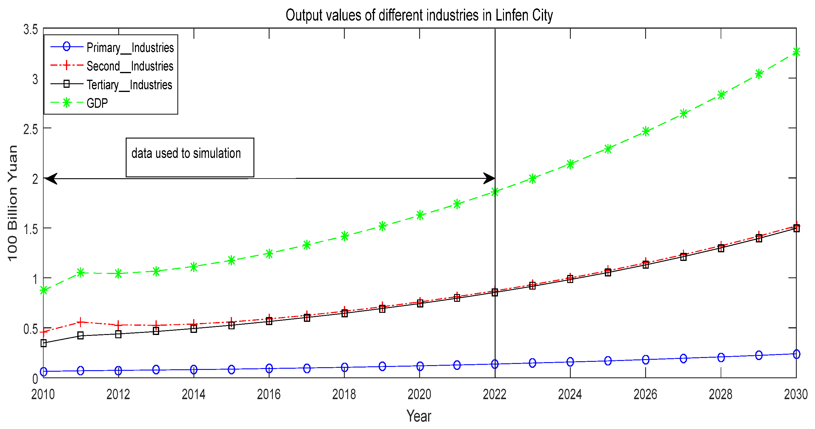
3.2.1. The Forecasting Results of GDP

Taking into account factors such as technological advancement, economic size, policy changes, and the overall GDP of the nation, we discovered that the electricity demand in Linfen City is expected to experience further growth in the future. By integrating the model’s features with the economic development trends and power consumption factors in Linfen City, the improved MGM (1, n) model was employed to forecast both the city’s GDP and its overall power consumption. The forecasting results and simulation data of different industries in Linfen City are shown in

Table 6. Forecasting results of GDP, the primary, secondary, and tertiary industries of Linfen City (CNY 100 billion).

Year	Primary Industry	Secondary Industry	Tertiary Industries	GDP
2023	0.148056	0.932828	0.916491	1.997375
2024	0.158663	0.999766	0.982936	2.141365
2025	0.170074	1.071757	1.054226	2.296056
2026	0.182338	1.149116	1.130707	2.462161
2027	0.195512	1.232199	1.212752	2.640464
2028	0.209658	1.321395	1.300762	2.831814
2029	0.224841	1.417126	1.395167	3.037135
2030	0.241135	1.519854	1.496431	3.25742

and Figure 3. The interpolation coefficients of the simulation model are 0.8032, 0.8920, and 0.6983, respectively. The GDP is estimated at CNY 325.74 billion in 2030. The primary, secondary, and tertiary industries in Linfen City are CNY 24.1 billion, CNY 152 billion, and CNY 149.6 billion, respectively (see Figure 1).

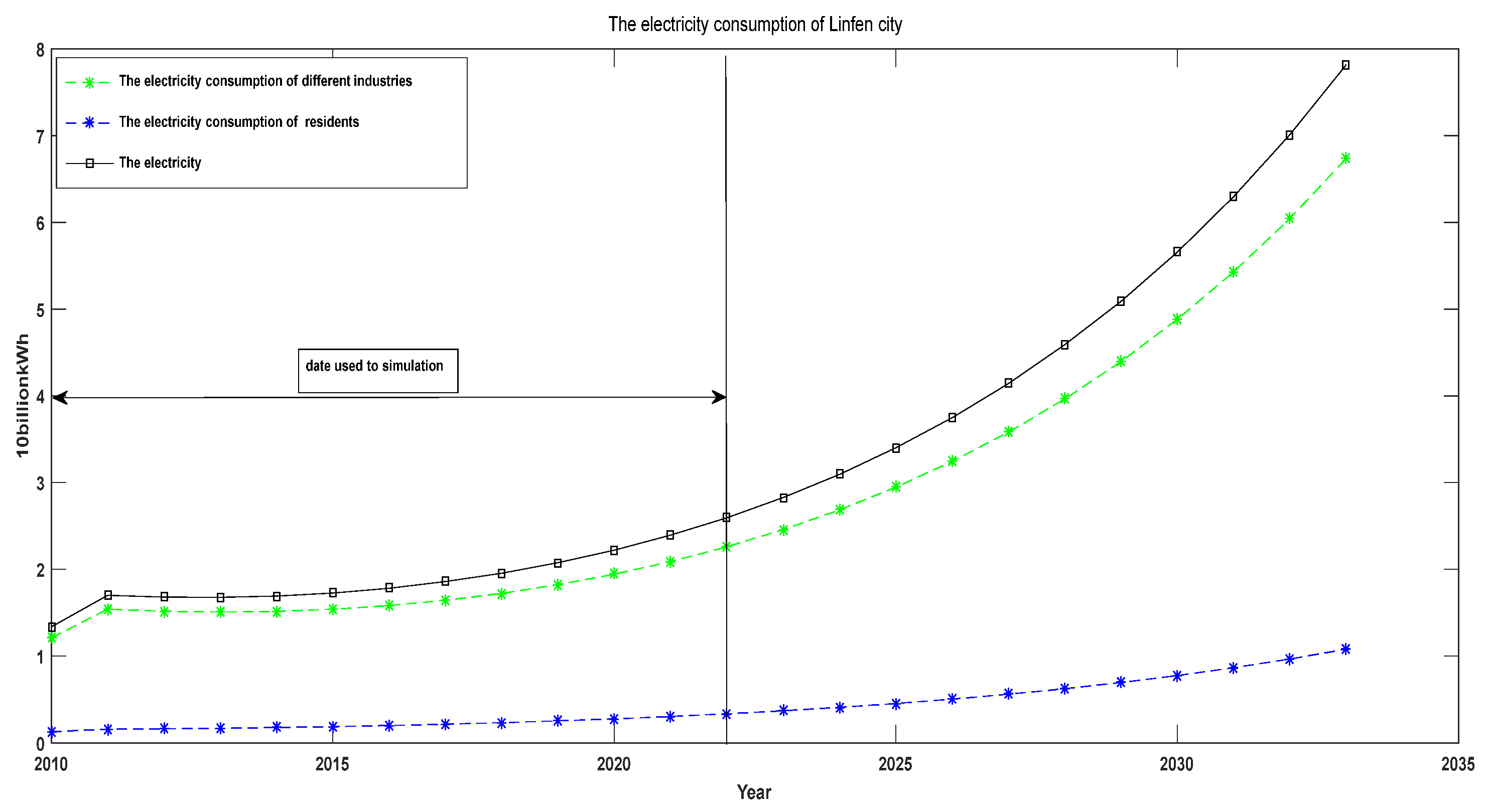
3.2.2. Prediction of Electricity Consumption in Linfen City

The forecasting results and simulation data of electricity consumption of Linfen City are shown in

Table 7. Prediction of electricity consumption in Linfen City.

Year	${\mathit{E}}_{\mathit{I}}$ (100 Billion kWh)	${\mathit{E}}_{\mathit{r}}$ (100 Billion kWh)	$\mathit{E}$ (100 Billion kWh)
2023	2.450	0.368	2.818
2024	2.678	0.408	3.086
2025	2.939	0.452	3.391
2026	3.236	0.5020	3.738
2027	3.572	0.558	4.13
2028	3.953	0.621	4.574
2029	4.382	0.692	5.074
2030	4.866	0.771	5.637

and Figure 4. The interpolation coefficients of the simulation model are 0.4735 and 0.4626. According to Table 6, by 2030, the residential electricity demand and industrial electricity demand of Linfen City are expected to go up to 77.1 billion kWh and, 486.7 billion kWh, respectively. This means that ensuring the safety of electric energy in Linfen City without increasing coal-fired power is an urgent problem to be solved.

4. Conclusions

In this article, we examine the driving factors and development trends of power consumption in Linfen City. The LMDI method was used to factorize the driving factors of power consumption. The results showed that the economic scale was firmly correlated to the industrial electricity demand. The technological level and GDP promoted industrial electricity consumption. This also illustrates a significant reliance of Linfen’s economy on coal-based industry, coupled with the sluggish pace of economic transformation and development. The technology level and GNP were the main factors promoting the growth of residential electricity demand. This implies that with the continued growth of GDP and the development of technology, social demand for electricity will increase in the future.

The improved MGM (1, n) model is used to predict the time series of GDP and electricity consumption for multiple indicators. The forecasting results show that by 2030, the GDP of Linfen City will be expected to pass CNY 325.74 billion, and the residential electricity demand and industrial electricity demand are expected to go up to 77.1 billion kWh and 486.7 billion kWh, respectively. Under the constraints of carbon peaking and carbon neutrality, ensuring the safety of electric energy in Linfen City while not increasing coal power is an urgent problem to be solved. However, Linfen City possesses abundant untapped clean energy resources, including hydropower, wind power, solar energy, and biomass energy. Currently in Linfen City, a significant amount of plant straw goes unprocessed, with much of it piled on farmland or directly burned, which can result in air pollution or an increase in pests, diseases, and grass infestations the following year. By harnessing the potential of straw to generate electricity, such issues can be mitigated. To resolve the contradiction between economic development and carbon dioxide emissions, the government needs to increase investments in clean energy infrastructure and develop clean power sources such as wind power, solar power, and biomass energy generation. At the same time, Linfen City should accelerate industrial transformation and adjust its industrial structure. Thus, the efficiency of power utilization will be improved and the output per unit power consumption will be increased. Compared with single-variable prediction models, the improved MGM (1, n) model can be used for multivariate time series prediction, generally applicable to cases with a limited number of variables. When there are too many variables with varying characteristics, this can increase the model’s complexity and affect its feasibility. In the next step, we will explore the relationship between the model and the variables.

References

1. Somu, N.; Raman, G.; Ramamritham, K. A deep learning framework for building energy consumption forecast. TERI Inf. Dig. Energy Environ. 2021, 1, 20. [Google Scholar] [CrossRef]
2. Juan, M.; Vikram, P.; Bidisha, G. A spiking neural network based wind power forecasting model for neuromorphic devices. Energies 2022, 15, 7256. [Google Scholar] [CrossRef]
3. Wen, M.; Yu, Z.C.; Li, W.Y.; Luo, S.C.; Zhong, Y.; Chen, C.Q. Short-term load forecasting based on feature mining and deep learning of big data of user electricity consumption. AIP Adv. 2023, 13, 125315. [Google Scholar] [CrossRef]
4. Eskandar, E.M.; Alammal, H.; Almadany, W. What prophet says about electrical consumption—Forecasting techniques for big temporal data. IET Conf. Proc. 2020, 2020, 543–548. [Google Scholar]
5. Amalou, I.; Mouhni, N.; Abdali, A. Multivariate time series prediction by RNN architectures for energy consumption forecasting. Energy Rep. 2022, 8, 1084–1091. [Google Scholar] [CrossRef]
6. Chen, H.Y.; Le, C.H.; Huang, B.M. Electricity consumption forecasting of buildings using hierarchical ANFIS and GRA. In Proceedings of the 2019 International Conference on Machine Learning and Cybernetics (ICMLC), Kobe, Japan, 7–10 July 2019. [Google Scholar]
7. Wen, L.; Song, Q. The forecasting model research of rural energy transformation in Henan Province based on STIRPAT model. Environ. Sci. Pollut. Res. Int. 2022, 29, 75550–75565. [Google Scholar] [CrossRef] [PubMed]
8. Nadja, K.; Michael, S.S.; David, J.N. Deep distributional time series models and the probabilistic forecasting of intraday electricity prices. J. Appl. Econom. 2023, 38, 493–511. [Google Scholar]
9. Zhan, L.P.; Gu, Y. Research on multi-scenario intelligent forecasting model of china’s electric power consumption driven by policy. IOP Conf. Ser. Earth Environ. Sci. 2019, 332, 042020. [Google Scholar] [CrossRef]
10. Zhao, H.; Guo, S. An optimized grey model for annual power load forecasting. Energy 2016, 107, 272–286. [Google Scholar] [CrossRef]
11. Wang, Z.X. A predictive analysis of clean energy consumption, economic growth and environmental regulation in China using an optimized grey dynamic model. Comput. Econ. 2015, 46, 437–453. [Google Scholar] [CrossRef]
12. Wang, Z.X.; Hao, P. An improved grey multivariable model for predicting industrial energy consumption in China. Appl. Math. Model. 2016, 40, 5745–5758. [Google Scholar] [CrossRef]
13. Wang, Z.X.; Li, Q.; Pei, L.L. Grey forecasting method of quarterly hydropower production in China based on a data grouping approach. Appl. Math. Model. 2017, 51, 302–316. [Google Scholar] [CrossRef]
14. Lee, Y.S.; Tong, L.I. Forecasting energy consumption using a grey model improved by incorporating genetic programming. Energy Convers. Manag. 2011, 52, 147–152. [Google Scholar] [CrossRef]
15. Wang, Z.X.; Ye, D.J. Forecasting Chinese carbon emissions from fossil energy consumption using non-linear grey multivariable models. J. Clean. Prod. 2017, 142, 600–612. [Google Scholar] [CrossRef]
16. Feng, Z.X.; Zhang, M.Q.; Wei, N.; Zhao, J.T.; Zhang, T.L.; He, X. An office building energy consumption forecasting model with dynamically combined residual error correction based on the optimal model. Energy Rep. 2022, 8, 12442–12455. [Google Scholar] [CrossRef]
17. Mehrnoosh, T.; Sattar, H.; Reza, S.M.; Shahaboddin, S.; Amir, M. A hybrid clustering and classication technique for forecasting short-term energy consumption. Environ. Prog. Sustain. Energy 2018, 38, 66–76. [Google Scholar]
18. Succetti, F.; Luzio, F.D.; Ceschini, A.; Rosato, A.; Araneo, R.; Panella, M. Multivariate prediction of energy time series by autoencoded LSTM networks. In Proceedings of the 2021 IEEE International Conference on Environment and Electrical Engineering and 2021 IEEE Industrial and Commercial Power Systems Europe (EEEIC/I&CPS Europe), Bari, Italy, 7–10 September 2021. [Google Scholar]
19. Magazzino, C.; Mutascu, M.; Mele, M.; Sarkodie, S.A. Energy consumption and economic growth in Italy: A wavelet analysis. Energy Rep. 2021, 7, 1520–1528. [Google Scholar] [CrossRef]
20. Chen, M.Y. Decoupling of energy consumption from economic growth in BRICS in the context of novel coronavirus pneumonia based on tapio decoupling index. Basic Clin. Pharmacol. Toxicol. 2020, 127, 238. [Google Scholar]
21. Kong, L.; Mu, X.; Hu, G. A decomposing analysis of productive and residential energy consumption in Beijing. Energy 2021, 226, 120413. [Google Scholar]
22. Liu, X.; Zhou, D.; Zhou, P.; Wang, Q. Factors driving energy consumption in China: A joint decomposition approach. J. Clean. Prod. 2018, 172, 724–734. [Google Scholar] [CrossRef]
23. Rocío, R.C.; Colinet, M.J. Are labor productivity and residential living standards drivers of the energy consumption changes? Energy Econ. 2018, 74, 746–756. [Google Scholar]
24. Ge, Y.H.; Yuan, R. Exploring decoupling relationship between ICT investments and energy consumption in China’s provinces: Factors and policy implications. Energy 2024, 286, 129506. [Google Scholar] [CrossRef]
25. Wang, W.X.; Zhang, W.; Cui, H.R.; Liu, B. Application of grey multi-variable model MGM (1, n) in the R & D investment forecast. RD Manag. 2006, 18, 92–96. [Google Scholar]
26. Wang, F.X. Multivariable non-equidistance MGM (1, m) model and its application. Syst. Eng. Electron. 2007, 29, 389–390. [Google Scholar]
27. Xiong, P.P.; Dang, Y.G.; Wang, Z.X. Optimization of background value in MGM (1, m) model. Control Decis. 2011, 26, 806–815. [Google Scholar]
28. Chen, C.P.; Liu, F.X.; Xu, Z.D. The research on optimized multi-variable grey model and its application. Math. Pract. Theory 2016, 46, 199–205. [Google Scholar]
29. Xiong, P.P.; Dang, Y.G.; Shu, H. Research on characteristics of MGM (1, m) model. Control Decis. 2012, 26, 389–393. [Google Scholar]
30. Wu, L.; Zhang, Z. Grey multivariable convolution model with new information priority accumulation. Appl. Math. Model. 2018, 62, 595–604. [Google Scholar] [CrossRef]
31. Ma, X.; Hu, Y.S.; Liu, Z.B. A novel kernel regularized nonhomogeneous grey model and its applications. Commun. Nonlinear Sci. Numer. Simul. 2017, 48, 51–62. [Google Scholar] [CrossRef]
32. Zeng, L. Analysing the high-tech industry with a multivariable grey forecasting model based on fractional order accumulation. Kybernetes 2018, 48, 1158–1174. [Google Scholar] [CrossRef]
33. Kenndy, J.; Eberhart, R.C. Particle swarm optimization. In Proceedings of the IEEE International Conference on Neural Networks, Perth, Australia, 27 November–1 December 1995; Volume 4, pp. 1942–1948. [Google Scholar]
Figure 1. The methodological diagram of the MGM (1, n) model.
Energies 17 03872 g001
Figure 2. The fitness cure of the improved MGM (1, 2).
Energies 17 03872 g002
Figure 3. Scatter diagram output values of different industries in Linfen City (2010–2030).
Energies 17 03872 g003
Figure 4. Scatter diagram of different electricity demand (2010–2030).
Energies 17 03872 g004