
Thermal Analysis of Parabolic and Fresnel Linear Solar Collectors Using Compressed Gases as Heat Transfer Fluid in CSP Plants

 ,
,  ,
,
Abstract
1. Introduction
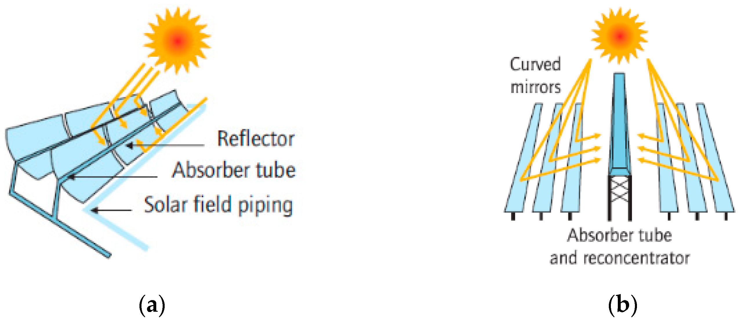
2. Parabolic Trough Collectors Modelling
2.1. Optical Model
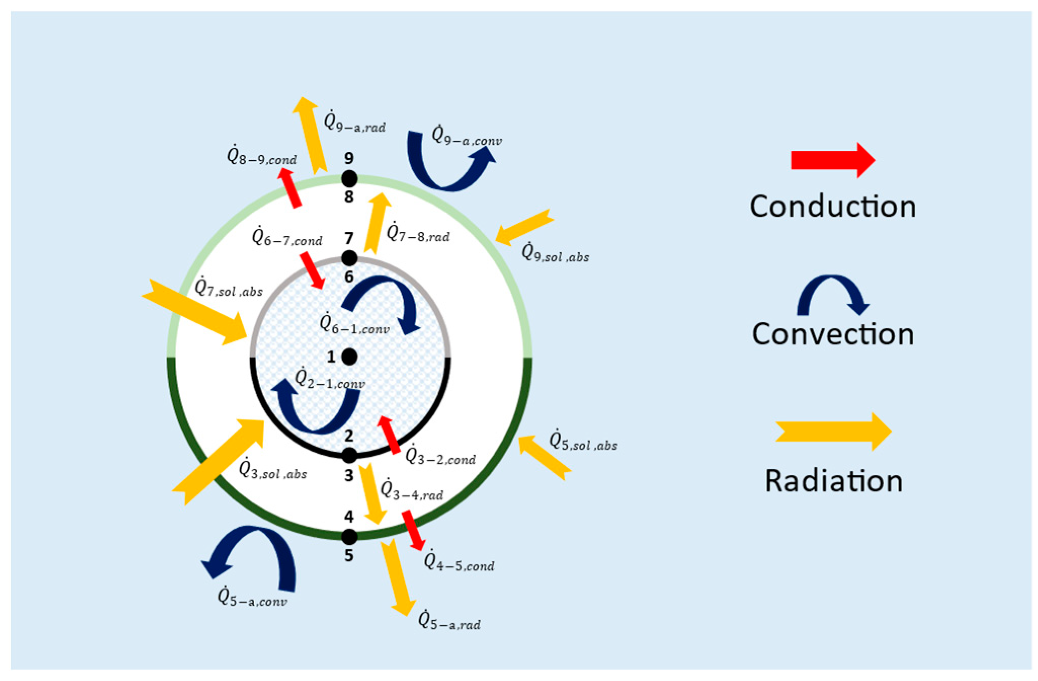
2.2. Thermal Model
- Conservation of mass:
- First law of thermodynamics:
- Conservation of mechanical energy: ;
- Convection heat transfer from inner surfaces of the absorber tube to the HTF, according to Newton’s law of cooling: , with
- (a)
- Computation of the convective heat transfer coefficient between the lower part of the glass envelope and the external environment in non-windy cases
- (b)
- Computation of the convective heat transfer coefficient between the upper part of the glass envelope and the external environment in non-windy cases
- (a)
- Computation of the convective heat transfer coefficient between the lower part of the glass envelope and the external environment in windy cases
- (b)
- Computation of the convective heat transfer coefficient between the upper part of the glass envelope and the external environment in windy cases
3. Linear Fresnel Collector Modelling
3.1. Optical Model
- Reducing the absorber’s radiation intensity based on the glass’ overall transmittance.
- Introducing a volumetric source within the glass, representing overall absorbance and mirroring the receiver’s angular radiation distribution.
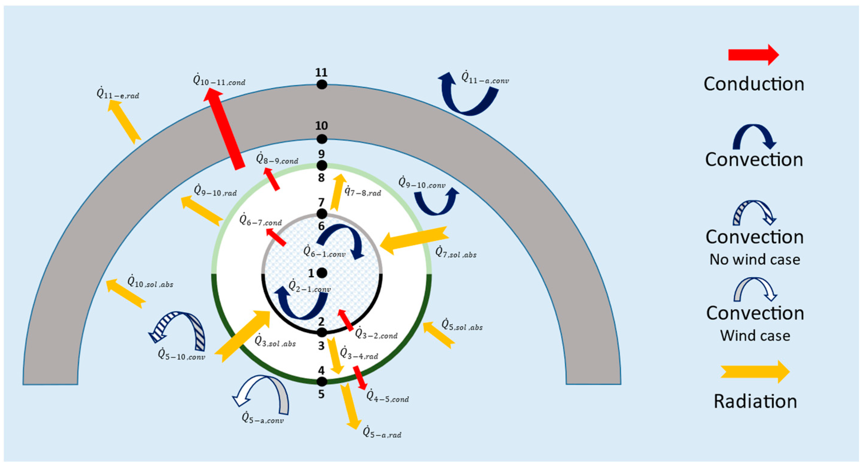
3.2. Thermal Model
- (a)
- Computation of the convective heat transfer coefficient between the lower part of the glass envelope and the external environment in non-windy cases
- (b)
- Computation of the convective heat transfer coefficient between the upper part of the glass envelope and the external environment in non-windy cases
- (c)
- Computation of the convective heat transfer coefficient between the CPC back casing and the external environment in non-windy cases
- (a)
- Computation of the convective heat transfer coefficient between the lower part of the glass envelope and the external environment in windy cases
- (b)
- Computation of the convective heat transfer coefficient between the upper part of the glass envelope and the external environment in windy cases
- (c)
- Computation of the convective heat transfer coefficient between the CPC back casing and the external environment in windy cases
4. Parabolic Trough Models Application for Thermal Performance Evaluation
4.1. Optical Model Results
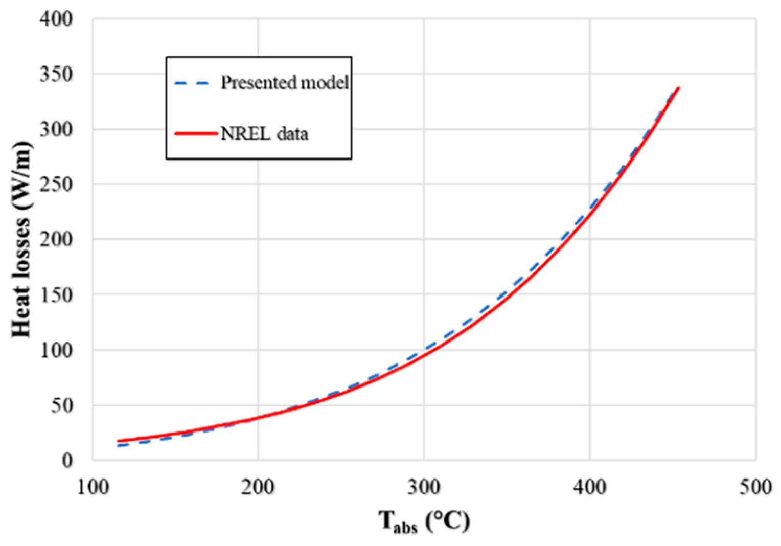
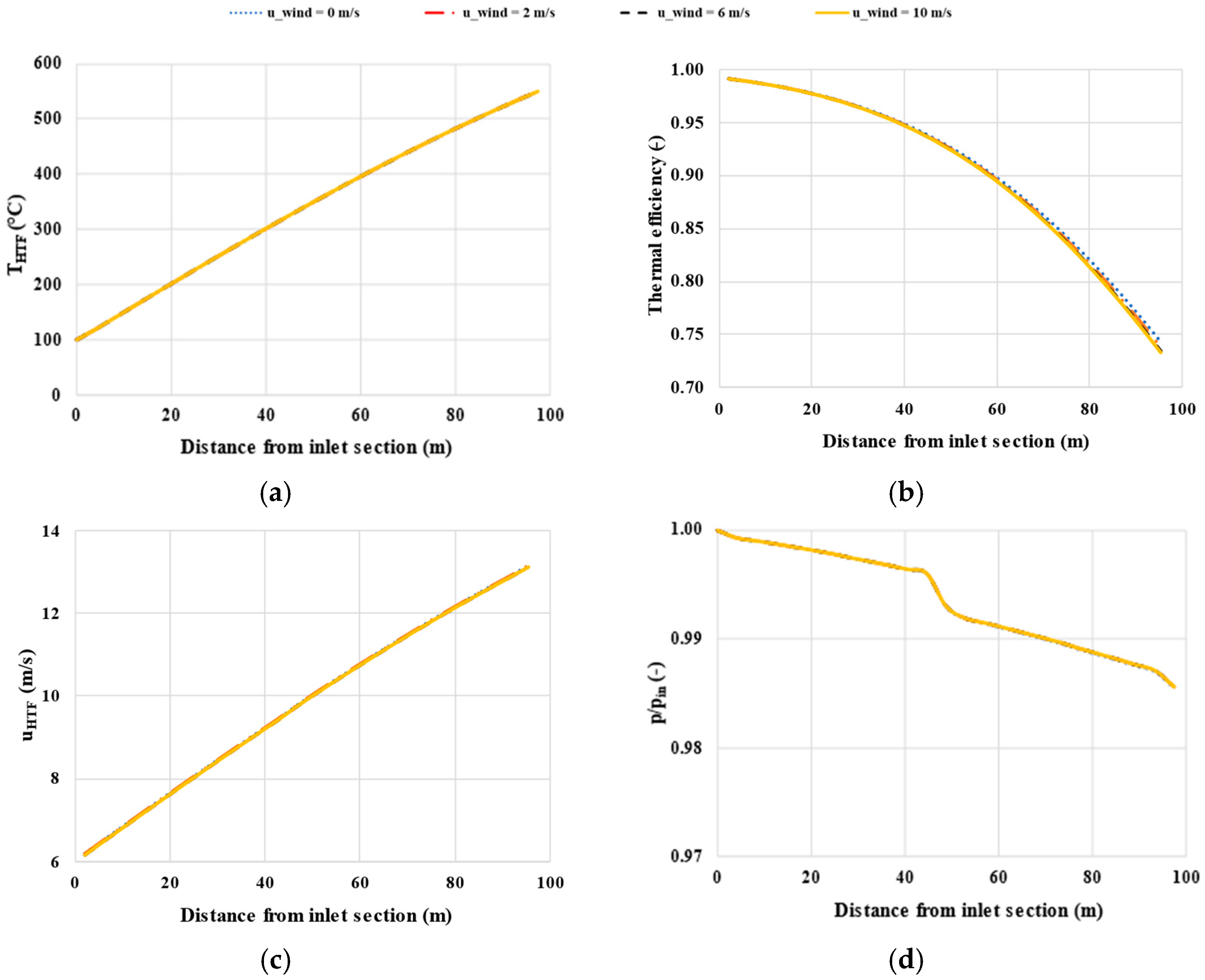
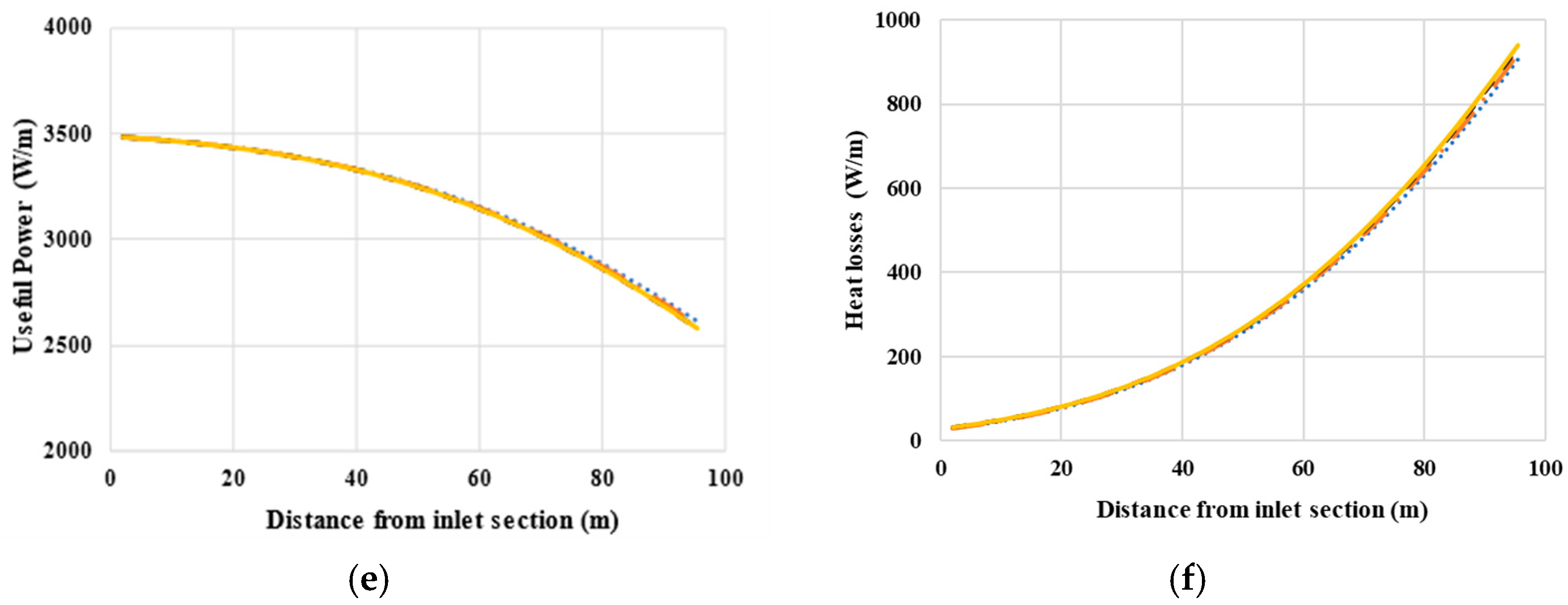
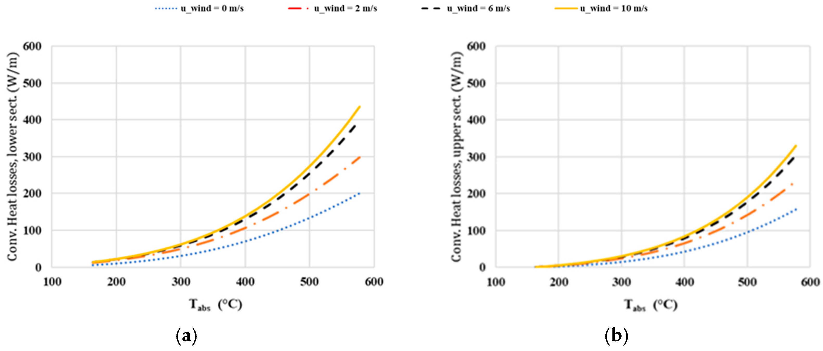
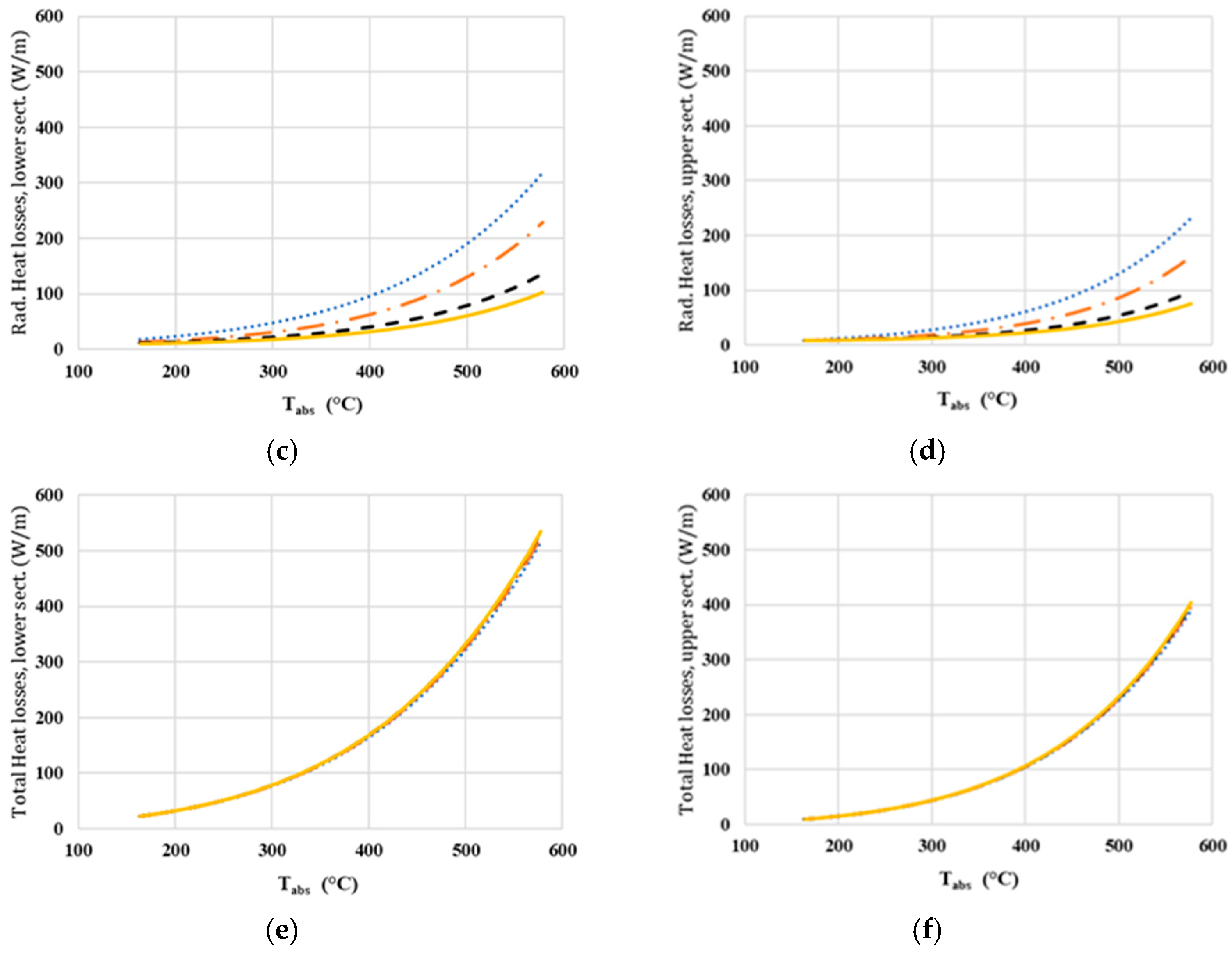
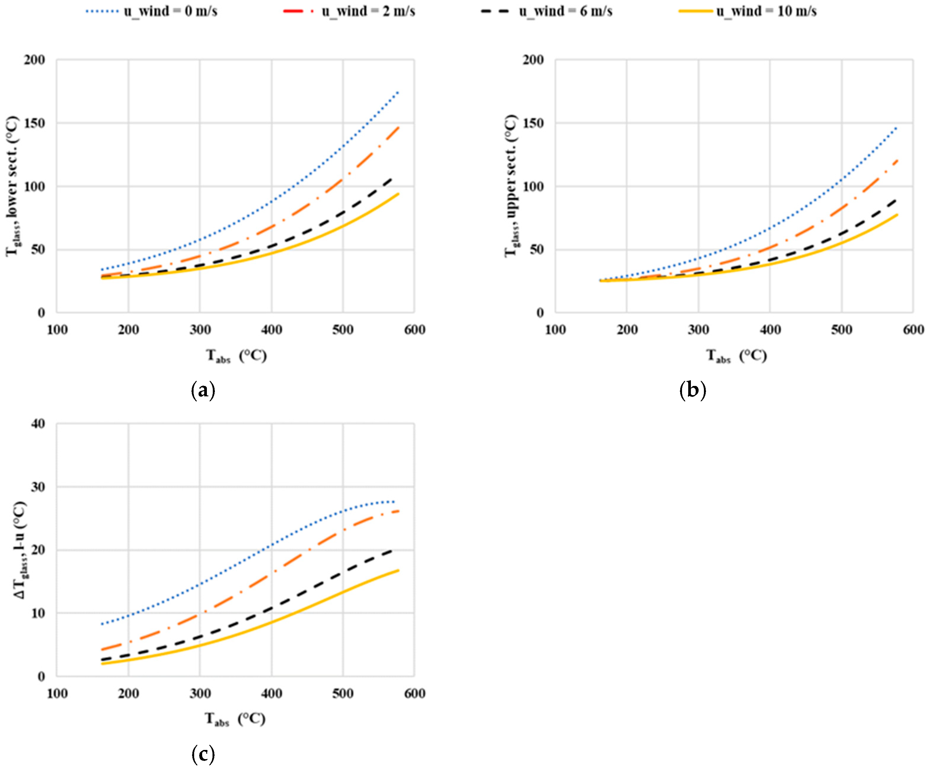
4.2. Thermal Model Results
- Glass Temperature Gradient: The difference between the lower and upper zone glass temperatures obviously defines the temperature gradient across the glass envelope (Figure 8c). This gradient steadily increases throughout the temperature operating range of the receiver tube and becomes more significant as wind speed decreases.
5. Linear Fresnel Model’s Application for Thermal Performance Evaluation
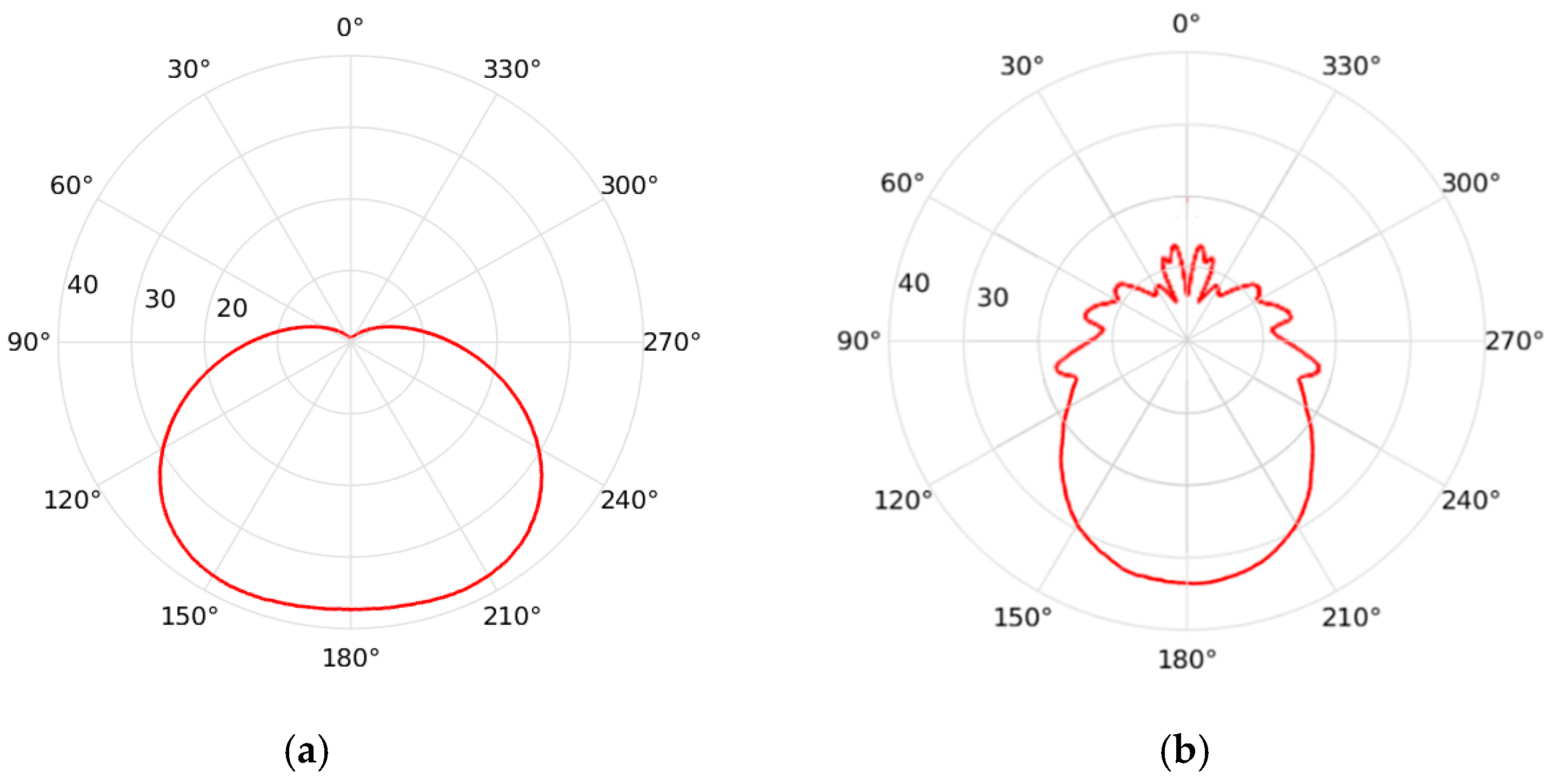
5.1. Optical Model Results
- Longitudinal incidence: 30° (along the collector axis);
- Transversal incidence: 0° (representing solar noon);
- Error standard deviation: 0.2°.
- Glass absorption: 0.054%
- Secondary reflector absorption: 3.69%
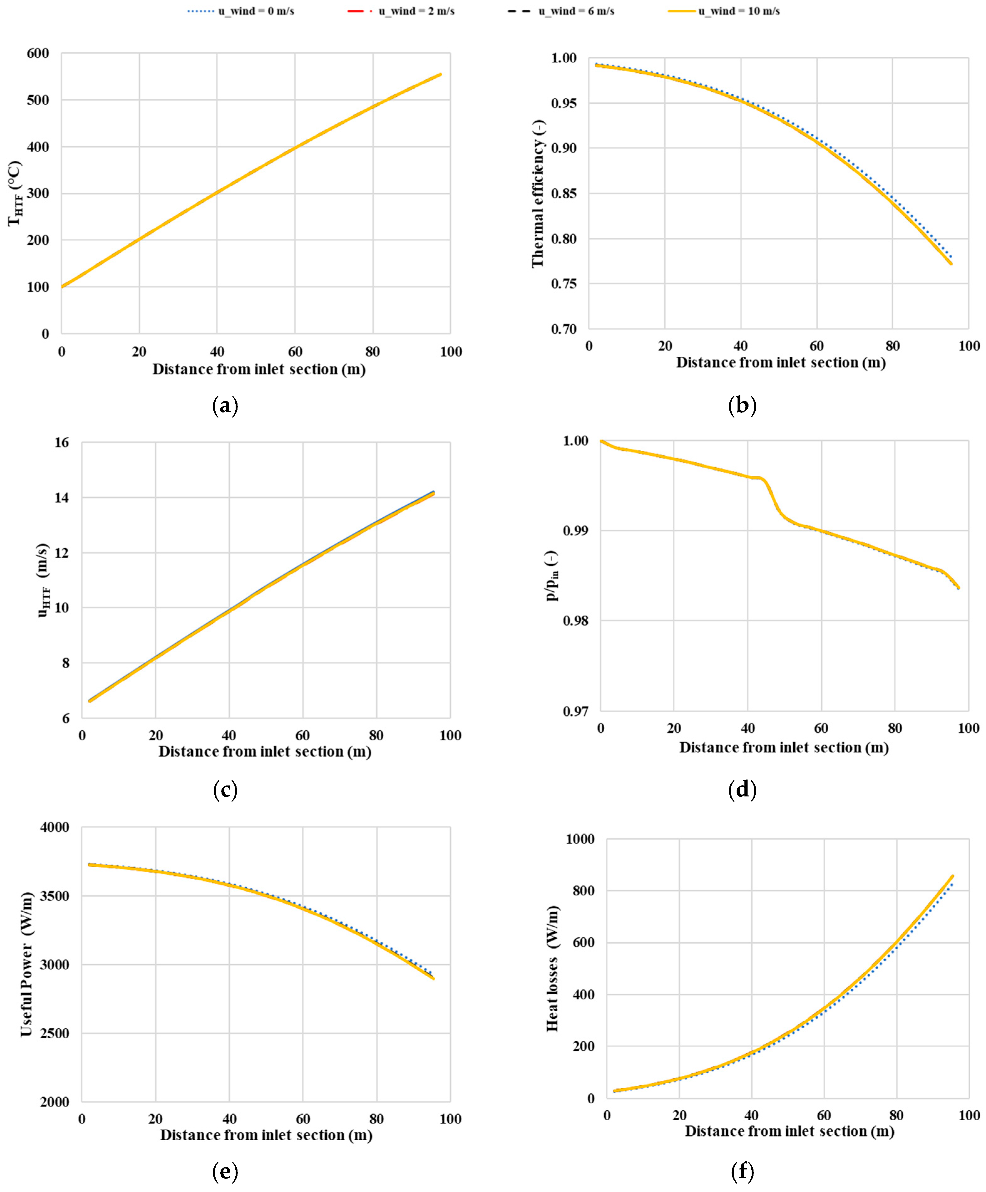
5.2. Thermal Model Results
6. Discussion
7. Conclusions
Author Contributions
Funding
Data Availability Statement
Conflicts of Interest
Nomenclature
| Abbreviations | |
| CSP | Concentrated Solar Power |
| HTF | heat transfer fluid |
| LFR | Linear Fresnel receiver |
| PT | Parabolic Trough |
| Symbols | |
| specific heat (W kg−1 K−1) | |
| diameter (m) | |
| kinetic energy (W) | |
| heat transfer coefficient (W m−2 K−1) | |
| enthalpy (W) | |
| thermal conductivity (W m−1 K−1) | |
| characteristic length (m) | |
| Nusselt number | |
| pressure (Pa) | |
| Prandtl number | |
| thermal power (W) | |
| useful power absorbed by HTF (W) | |
| heat losses to environment (W) | |
| radius (m) | |
| Rayleigh number | |
| Reynolds number | |
| Temperature (K) | |
| fluid velocity (m s−1); | |
| specific volume (m3 kg−1) | |
| Greek symbols | |
| thermal expansion coefficient (°C−1) | |
| ρ | density (kg m−3) |
| dynamic viscosity (Pa s) | |
| Subscripts and superscripts | |
| 1 | heat transfer fluid |
| 2 | absorber tube inner surface, lower half |
| 3 | absorber tube outer surface, lower half |
| 4 | glass envelope tube inner surface, lower half |
| 5 | glass envelope tube outer surface, lower half |
| 6 | absorber tube inner surface, upper half |
| 7 | absorber tube outer surface, upper half |
| 8 | glass envelope tube inner surface, upper half |
| 9 | glass envelope tube outer surface, upper half |
| 10 | secondary reflector inner surface |
| 11 | secondary reflector outer surface |
| a | external environment |
| abs | absorber tube |
| cond | conductive |
| conv | convective |
| eq | equivalent |
| HTF | heat transfer fluid |
| i | inner surface |
| in | collector inlet element |
| l | lower sector |
| o | outer surface |
| out | collector outlet element |
| rad | radiative |
| sol,abs | absorbed solar radiation |
| t | thermal |
| u | upper sector |
References
- Cabeza, L.F.; Galindo, E.; Prieto, C.; Barraneche, C.; Fernández, A.I. Key performance indicators in thermal energy storage: Survey and assessment. Renew. Energy 2015, 83, 820–827. [Google Scholar] [CrossRef]
- IEA. Technology Roadmap: Solar Thermal Electricity, 2014th ed.; International Energy Agency: Paris, France, 2014. [Google Scholar]
- Esposito, S.; D’Angelo, A.; Antonaia, A.; Castaldo, A.; Ferrara, M.; Addonizio, M.L.; Guglielmo, A. Optimization procedure and fabrication of highly efficient and thermally stable solar coating for receiver operating at high temperature. Sol. Energy Mater. Sol. Cells 2016, 157, 429–437. [Google Scholar] [CrossRef]
- Falchetta, M.; Gambarotta, A.; Vaja, I.; Cucumo, M.; Manfredi, C. Modelling and Simulation of the Thermo and Fluid Dynamics of the “Archimede Project” Solar Power Station. Renew. Energy Process. Syst. 2006, 3, 1499–1506. [Google Scholar]
- Giaconia, A.; Iaquaniello, G.; Metwally, A.A.; Caputo, G.; Balog, I. Experimental demonstration and analysis of a CSP plant with molten salt heat transfer fluid in parabolic troughs. Sol. Energy 2020, 211, 622–632. [Google Scholar] [CrossRef]
- Liberatore, R.; Giaconia, A.; Petroni, G.; Caputo, G.; Felici, C.; Giovannini, E.; Giorgetti, M.; Branke, R.; Mueller, R.; Karl, M.; et al. Analysis of a procedure for direct charging and melting of solar salts in a 14 MWh thermal energy storage tank. AIP Conf. Proc. 2019, 2126, 200024. [Google Scholar]
- Grena, R.; Tarquini, P. Solar linear Fresnel collector using molten nitrates as heat transfer fluid. Energy 2011, 36, 1048–1056. [Google Scholar] [CrossRef]
- Falchetta, M.; Mazzei, D.; Russo, V.; Campanella, V.A.; Floridia, V.; Schiavo, B.; Venezia, L.; Brunatto, C.; Orlando, R. The Partanna project: A first of a kind plant based on molten salts in LFR collectors. AIP Conf. Proc. 2020, 2303, 040001. [Google Scholar]
- Concentrating Solar Power Projects|NREL. Available online: https://solarpaces.nrel.gov/ (accessed on 12 June 2024).
- Fernandez-Garcia, A.; Zarza, E.; Valenzuela, L.; Perez, M. Parabolic-trough Solar Collectors and Their Applications. Renew. Sustain. Energy Rev. 2010, 14, 1695–1721. [Google Scholar] [CrossRef]
- Benoit, H.; Spreafico, L.; Gauthier, D.; Flamant, G. Review of Heat Transfer Fluids in Tube-Receivers Used in Concentrating Solar Thermal Systems: Properties and Heat Transfer Coefficients. Renew. Sust. Energy Rev. 2016, 55, 298–315. [Google Scholar] [CrossRef]
- Krishna, Y.; Faizal, M.; Saidur, R.; Ng, K.C.; Aslfattahi, N. State-of-the-art Heat Transfer fluids for Parabolic Trough Collector. Int. J. Heat Mass Transf. 2020, 152, 119541. [Google Scholar] [CrossRef]
- Muñoz-Anton, J.; Biencinto, M.; Zarza, E.; Díez, L.E. Theoretical basis and experimental facility for parabolic trough collectors at high temperature using gas as heat transfer fluid. Appl. Energy 2014, 135, 373–381. [Google Scholar] [CrossRef]
- IEA. Technology Roadmap: Concentrating Solar Power, 2010th ed.; International Energy Agency: Paris, France, 2010. [Google Scholar]
- Grena, R. Optical simulation of a parabolic solar trough collector. Int. J. Sust. Energy 2010, 29, 19–36. [Google Scholar] [CrossRef]
- Forristall, R. Heat Transfer Analysis and Modeling of a Parabolic Trough Solar Receiver Implemented in Engineering Equation Solver; Technical report-OSTI ID: 15004820; U.S. Department of Energy, Office of Scientific and Technical Information: Oak Ridge, TN, USA, 2003. [Google Scholar]
- Churchill, S.W.; Chu, H.H.S. Correlating equations for laminar and turbulent free convection from a horizontal cylinder. Int. J. Heat Mass Transf. 1975, 18, 1049–1053. [Google Scholar] [CrossRef]
- Zukauskas, A. Heat transfer from tubes in cross flow. Adv. Heat Transf. 1972, 8, 93–160. [Google Scholar]
- Raithby, G.D.; Hollands, K.G.T. A general method of obtaining approximate solutions to laminar and turbulent free convection problems. Adv. Heat Transf. 1975, 11, 265–315. [Google Scholar]
- Montes, M.J.; Barbero, R.; Abbas, R.; Rovira, A. Performance model and thermal comparison of different alternatives for the Fresnel single-tube receiver. Appl. Therm. Eng. 2016, 104, 162–175. [Google Scholar] [CrossRef]
- Reddy, K.S.; Shanmugapriya, B.; Sundararajan, T. Estimation of heat losses due to wind effects from linear parabolic secondary reflector—Receiver of solar LFR module. Energy 2018, 150, 410–433. [Google Scholar] [CrossRef]
- Reddy, K.S.; Shanmugapriya, B.; Sundararajan, T. Heat loss investigation of 125kWth solar LFR pilot plant with parabolic secondary evacuated receiver for performance improvement. Int. J. Therm. Sci. 2018, 125, 324–341. [Google Scholar] [CrossRef]
- Balaji, S.; Reddy, K.S.; Sundararajan, T. Performance investigation of linear evacuated absorber of 2-stage solar Linear Fresnel Reflector module under non-uniform flux distribution. Int. J. Low-Carbon Technol. 2018, 13, 92–101. [Google Scholar]
- Hilpert, R. Wärmeabgabe von geheizten Drähten und Rohren im Luftstrom. Forsch. Gebiet Ingenieurw. 1933, 4, 215–224. [Google Scholar] [CrossRef]
- Burkholder, F.W.; Kutscher, C.F. Heat-Loss Testing of Solel’s UVAC3 Parabolic Trough Receiver; Technical report NREL/TP-550-42394; National Renewable Energy Laboratory (NREL): Golden, CO, USA, 2008. [Google Scholar]
- Soltigua. 1 MWe CSP-ORC Pilot Plant, Solar Field Process Description; Report No.: S-F14ET001-M-B-A-2602-C; Soltigua SRL: Gambettola, Italy, 2015. [Google Scholar]


| Parameter | Unit | Value |
|---|---|---|
| Length of steel tube/absorber tube | m | 4.06 |
| Length of passive stubs mounted at the end of the manifold | m | 0.64 |
| Length of passive stubs mounted at the end of the triples of pipes | m | 0.155 |
| Length passive stubs mounted on the central area of the collector | m | 0.68 |
| Equivalent length of manifold connections to fixed piping | m | 7 |
| Equivalent length of the return pipe | m | 21 |
| Number of pipes making up a collector | m | 12 |
| Number of collectors making up the loop | - | 2 |
| Absorber tube outer diameter | m | 0.070 |
| Absorber tube thickness | m | 0.003 |
| Glass cover tube diameter | m | 0.125 |
| Glass cover tube thickness | m | 0.003 |
| Mirror reflectivity | - | 0.92 |
| Glass overall transmissivity (normal incidence) | - | 0.96 |
| Glass extinction coefficient | - | 0.000625 |
| Cermet absorbance | - | 0.95 |
| DNI (Direct Normal Irradiance) | W/m2 | 800 |
| Ambient temperature | °C | 25 |
| Ambient pressure | bar | 1 |
| Inlet temperature | °C | 225 |
| Inlet pressure | bar | 30 |
| Mass flow | kg/s | 0.93 |
| Cermet max temperature | °C | 600 |
| Loop length | m | 100 |
| Parameter | Unit | Value |
|---|---|---|
| Collector width | m | 5.9 |
| Collector focal length | m | 1.81 |
| Spacing between mirrors | m | 1.2 |
| Parameter | Unit | Value |
|---|---|---|
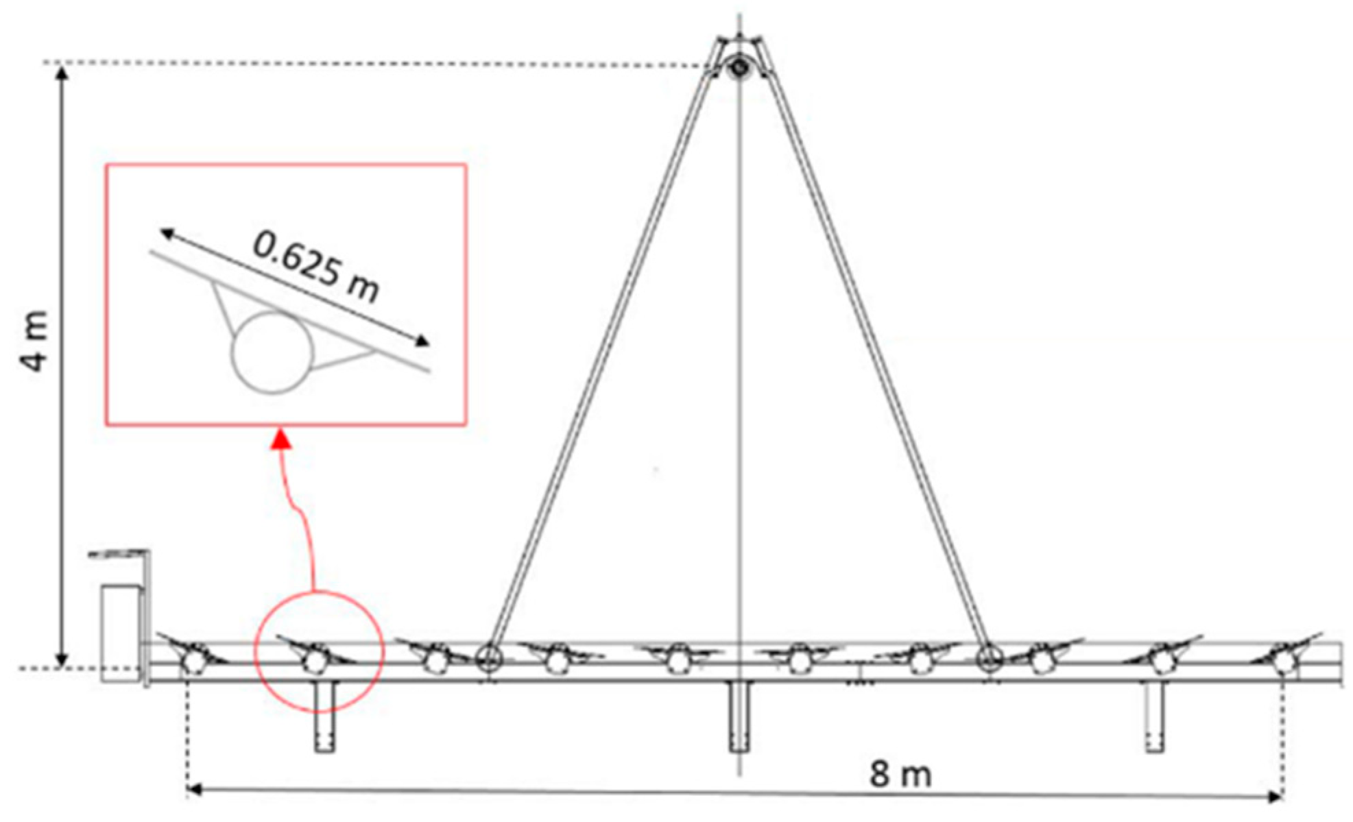
| Number of mirrors | - | 10 |
| Mirror width | m | 0.625 |
| Spacing factor between mirrors | m | 1.2 |
| Receiver height | m | 4 |
| Mirror focal length | m | 4.617 |
| CPC opening width | m | 0.29 |
| CPC opening height | m | 3.9375 |
| CPC height | m | 0.145 |
| Longer base of the insulating trapezium | m | 0.353 |
| Shorter base of the insulating trapezium | m | 0.18 |
| Height of the insulating trapezium | m | 0.1765 |
| Collector | Useful Power (kWth) | Heat Losses (kWth) | Thermal Efficiency (-) |
|---|---|---|---|
| PT | 310 | 32.8 | 0.904 |
| LFR | 335 | 30.6 | 0.916 |
Disclaimer/Publisher’s Note: The statements, opinions and data contained in all publications are solely those of the individual author(s) and contributor(s) and not of MDPI and/or the editor(s). MDPI and/or the editor(s) disclaim responsibility for any injury to people or property resulting from any ideas, methods, instructions or products referred to in the content. |
© 2024 by the authors. Licensee MDPI, Basel, Switzerland. This article is an open access article distributed under the terms and conditions of the Creative Commons Attribution (CC BY) license (https://creativecommons.org/licenses/by/4.0/).
Share and Cite
Grena, R.; Lanchi, M.; Frangella, M.; Ferraro, V.; Marinelli, V.; D’Auria, M. Thermal Analysis of Parabolic and Fresnel Linear Solar Collectors Using Compressed Gases as Heat Transfer Fluid in CSP Plants. Energies 2024, 17, 3880. https://doi.org/10.3390/en17163880
Grena R, Lanchi M, Frangella M, Ferraro V, Marinelli V, D’Auria M. Thermal Analysis of Parabolic and Fresnel Linear Solar Collectors Using Compressed Gases as Heat Transfer Fluid in CSP Plants. Energies. 2024; 17(16):3880. https://doi.org/10.3390/en17163880
Chicago/Turabian StyleGrena, Roberto, Michela Lanchi, Marco Frangella, Vittorio Ferraro, Valerio Marinelli, and Marco D’Auria. 2024. "Thermal Analysis of Parabolic and Fresnel Linear Solar Collectors Using Compressed Gases as Heat Transfer Fluid in CSP Plants" Energies 17, no. 16: 3880. https://doi.org/10.3390/en17163880
APA StyleGrena, R., Lanchi, M., Frangella, M., Ferraro, V., Marinelli, V., & D’Auria, M. (2024). Thermal Analysis of Parabolic and Fresnel Linear Solar Collectors Using Compressed Gases as Heat Transfer Fluid in CSP Plants. Energies, 17(16), 3880. https://doi.org/10.3390/en17163880