Article

Research into the Fast Calculation Method of Single-Phase Transformer Magnetic Field Based on CNN-LSTM

1
Electric Power Research Institute of Yunnan Power Grid Corporation, Kunming 650217, China
2
China Southern Power Grid Yunnan Power Grid Co., Ltd., Kunming 650217, China
3
Laboratory of Power Transmission Equipment Technology, Chongqing University, Shapingba District, Chongqing 400044, China
*
Author to whom correspondence should be addressed.
Energies 2024, 17(16), 3913; https://doi.org/10.3390/en17163913
Submission received: 12 May 2024 / Revised: 19 July 2024 / Accepted: 25 July 2024 / Published: 8 August 2024
(This article belongs to the Special Issue Electrical Engineering, High Voltage and Insulation Technology)

Abstract

:
Magnetic field is one of the basic data for constructing a transformer digital twin. The finite element transient simulation takes a long time and cannot meet the real-time requirements of a digital twin. According to the nonlinear characteristics of the core and the timing characteristics of the magnetic field, this paper proposes a fast calculation method of the spatial magnetic field of the transformer, considering the nonlinear characteristics of the core. Firstly, based on the geometric and electrical parameters of the single-phase double-winding test transformer, the corresponding finite element simulation model is built. Secondly, the key parameters of the finite element model are parametrically scanned to obtain the nonlinear working condition data set of the test transformer. Finally, a deep learning network integrating a convolutional neural network (CNN) and a long short-term memory network (LSTM) is built to train the mapping relationship between winding voltage, current, and the spatial magnetic field so as to realize the rapid calculation of the transformer magnetic field. The results show that the calculation time of the deep learning model is greatly shortened compared with the finite element model, and the model calculation results are consistent with the experimental measurement results.

1. Introduction

A digital twin is an important way to build the digitalization of electric power equipment and systems [1,2]. Transformers are one of the most significant pieces of equipment in power systems; building the digital twin of a transformer is an important task for the digitalization of power systems at the equipment level [3], which can achieve the real-time perception and prediction of transformer operation status and provide real-time data for state evaluation and rapid decision making.
The magnetic field distribution of a transformer is one of the key physical fields that determine its performance and operating status. The distribution of the leakage magnetic field during the normal operation of transformers has symmetry, and the characteristic quantities of winding leakage magnetic field distribution can be used to study the early faults of transformer [4]. Moreover, the online monitoring of transformer winding deformation and the determination of deformation type can also be achieved through magnetic field measurement [5]. The main magnetic flux can reflect the operating status of the transformer core. Grasping the distribution of the main magnetic flux can support the optimization of the design of the shape and size of the core [6], reduce magnetic flux loss, and improve the efficiency and technical economy of the transformer [7].
At present, the main methods for obtaining transformer magnetic fields can be divided into sensor measurement, finite element simulation, and algorithm inversion. Sensor measurement is mainly based on principles such as magnetic flux gates, electromagnetic induction coils, and the Hall effect to measure AC or DC magnetic fields [8]. However, magnetic field sensors have limitations including low sensitivity, high cost, and inflexibility in measurement positions [9], which can only obtain the magnetic field value of the measurement point rather than the distribution of the entire magnetic field. Finite element calculation can describe the complex magnetic field distribution characteristics inside transformers. The simulation results using mature commercial software such as ANSYS, Ansoft, COMSOL, and so on, which have high consistency with actual measurement results, and their accuracy has been verified by actual measurements and theoretical analysis [10]. However, power transformers are bulky, structurally complex, and have multi-scale characteristics in their internal components, resulting in finite element simulation taking hours [11], and with some 3D simulations taking days [12], making it difficult to meet the requirements of real-time measurement distribution and fast and efficient digital twins.
In recent years, with the increase in data, machine learning (ML) methods have been used to analyze data, find patterns, and make predictions. ANSYS developed a fast simulation module for multiple physical fields [13], which can train and obtain various transformer magnetic field reduction modules based on Twin Builder [14]. The latest version released by the COMSOL company has added a data-driven proxy model that provides strong support for digital twin models [15]. The research on deep learning algorithms in the field of transformers mainly focuses on magnetic field and temperature calculations [16,17,18]. For example, based on deep belief networks (DBNs) and transformer leakage magnetic field information, the fault type of transformers can be quickly identified [19]. Early faults can be quickly identified and located in windings based on the difference between the leakage magnetic field information output by the multi-state analytical model and the physically measured information [20]. A Support Vector Machine (SVM) [5] can be used to achieve the accurate classification of transformer winding deformation and to determine the deformation severity. The intrinsic orthogonal decomposition (POD) method and a deep neural network (DNN) can be used to accelerate finite element simulation. Deep neural networks (DL) can be used to predict the field distribution in electromagnetic devices [21]. The naive Bayesian algorithm can be used to evaluate the magnetic and electric fields for predicting electrostatic discharge [22]. The fast calculation of physical fields can be achieved based on U-net networks [23]. The above accelerated calculation and prediction methods can be used for the fast calculation of magnetic fields, but the nonlinearity of ferromagnetic materials and the differential distribution characteristics of spatial magnetic fields have been ignored in the research.
In summary, the above magnetic field calculation of transformers mainly considers the working conditions of the iron core working in the linear region. However, in actual operation, common disturbances such as power frequency overvoltage, DC bias, and excitation inrush current will increase the excitation current and saturate the iron core, causing the transformer to work in the nonlinear region. Changes in the internal magnetic field distribution characteristics of the transformer will cause the performance of existing fast calculation methods to deteriorate. For specific nonlinear operating conditions, the magnetic field distribution can usually only be obtained through finite element simulation with hourly counts, and it is difficult to meet the requirements of the calculation speed of building digital twins. Therefore, it is necessary to build a spatial magnetic field fast calculation model that takes into account the nonlinear characteristics of the iron core to meet the fast and accurate needs of digital twin research in the transformer equipment layer.
This paper proposes an accelerated computing model for the dual-branch training of a CNN-LSTM network to address the nonlinearity of transformer cores and the distribution characteristics of magnetic fields [24,25]. Firstly, the hysteresis model parameters of the single-phase dual-winding transformer are obtained through experiments, and then a finite element simulation model of the experimental transformer is established by combining other relevant parameters. Based on the finite element simulation model, parameterized scanning is performed to obtain a multi-operating condition data set of the experimental transformer, providing data support for the training of deep learning models. Finally, a CNN-LSTM deep learning network is trained based on the data set to achieve the fast calculation of the spatial magnetic field of transformers from hour level to second level, supporting the construction of digital twin models for transformers and the near-real-time visualization of spatial magnetic fields.

2. Construction and Verification of Finite Element Model for Single-Phase Transformer

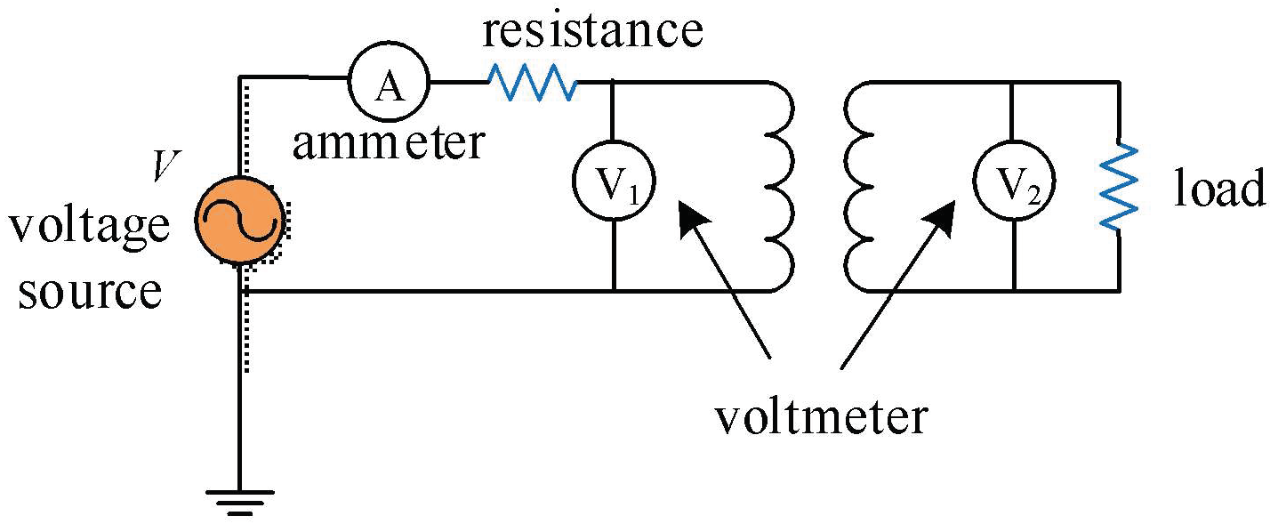
2.1. Single-Phase Transformer Test Platform and J-A Model Parameter Extraction

In order to achieve the synchronous measurement of transformer winding voltage, current, and spatial magnetic field, a magnetic field measurement test platform for a single-phase dual-winding transformer with a capacity of 50 VA was built in the laboratory. The instruments and equipment involved in the test are shown in Figure 1.
An arbitrary waveform generator combined with a power amplifier is used as power source excitation and is connected to the primary side of the transformer, with the secondary side unloaded. The voltage probe measures the voltage on the primary and secondary side, the current probe measures the current on the primary side, and the Gaussian meter measures the leakage flux in space. The measurement signal is collected simultaneously through a multi-channel high-speed acquisition card, and the waveform is displayed in real-time on the display screen. During the experiment, by adjusting the signal amplitude and bias of the arbitrary waveform generator to change its output waveform, the operating conditions of the transformer can be changed. The Hall probe of the Gaussian meter can be fixed at any position to measure the magnetic field at a spatial point. With the collaborative work of these instruments and collection systems, the real-time monitoring and recording of the voltage, current, and magnetic field data of transformers under different working conditions can be achieved, providing reliable data for the subsequent research and analysis of the magnetic field characteristics of single-phase transformer cores working in the nonlinear region.
By gradually increasing the output voltage amplitude of the arbitrary waveform generator, the data of transformers with iron cores operating at different saturation levels can be obtained. In order to establish a finite element simulation model that is consistent with the experimental transformer and analyze more operating conditions through finite element simulation, it is necessary to obtain the hysteresis model parameters of the iron core. This article uses the Jiles Atheron hysteresis model (J-A model) to describe the hysteresis effect of the iron core. By processing the experimental data under the saturation condition of the iron core, the BH curve of the test transformer can be obtained. The comparison between the BH curve of the transformer solved using the Particle Swarm Optimization (PSO) algorithm and the experimental BH curve is shown in Figure 2. The calculated J-A model parameters are shown in Table 1.

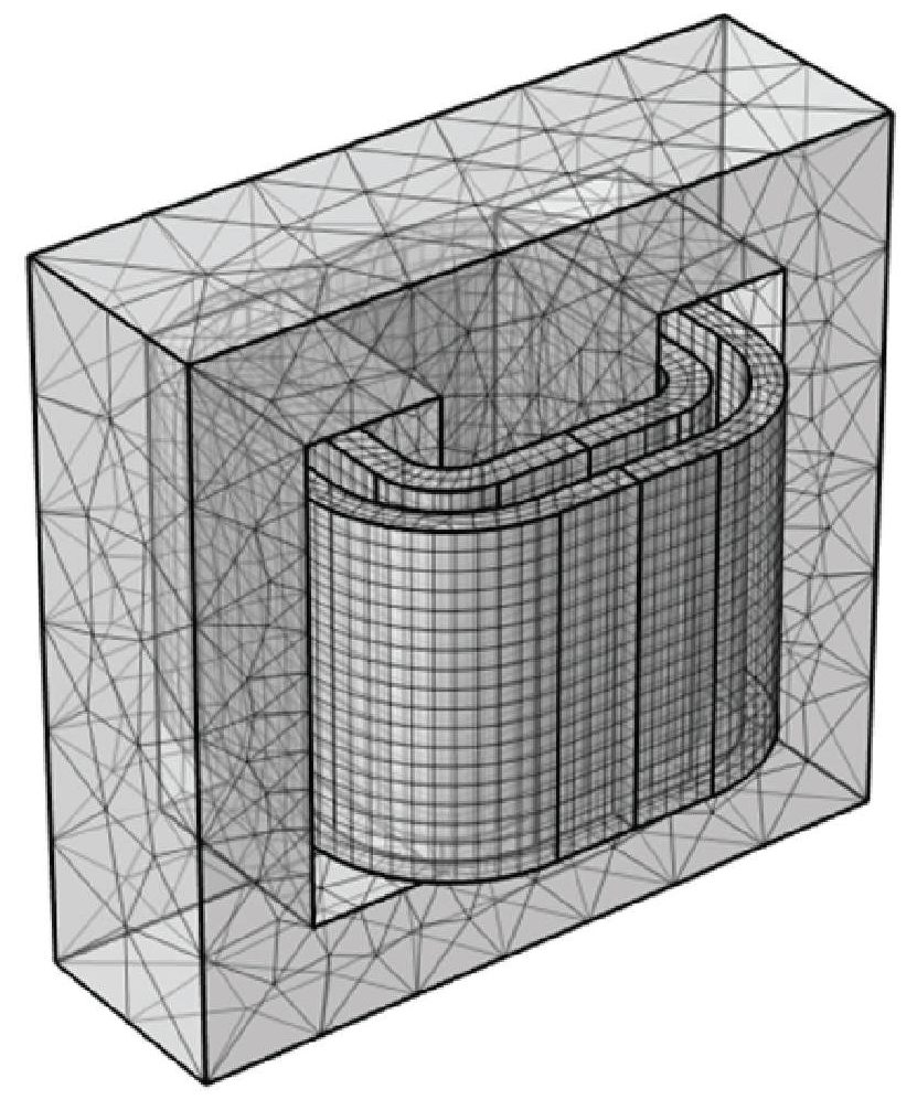
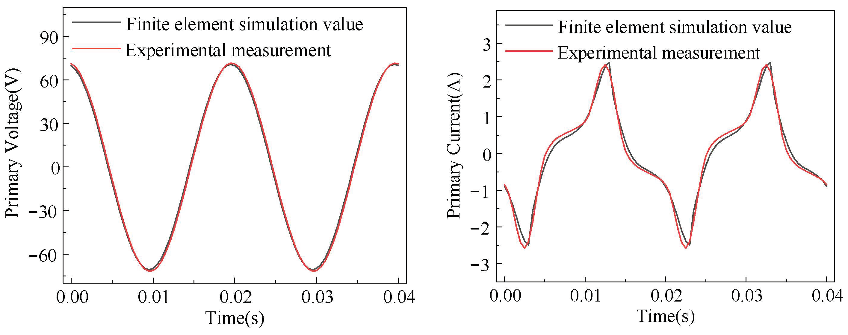
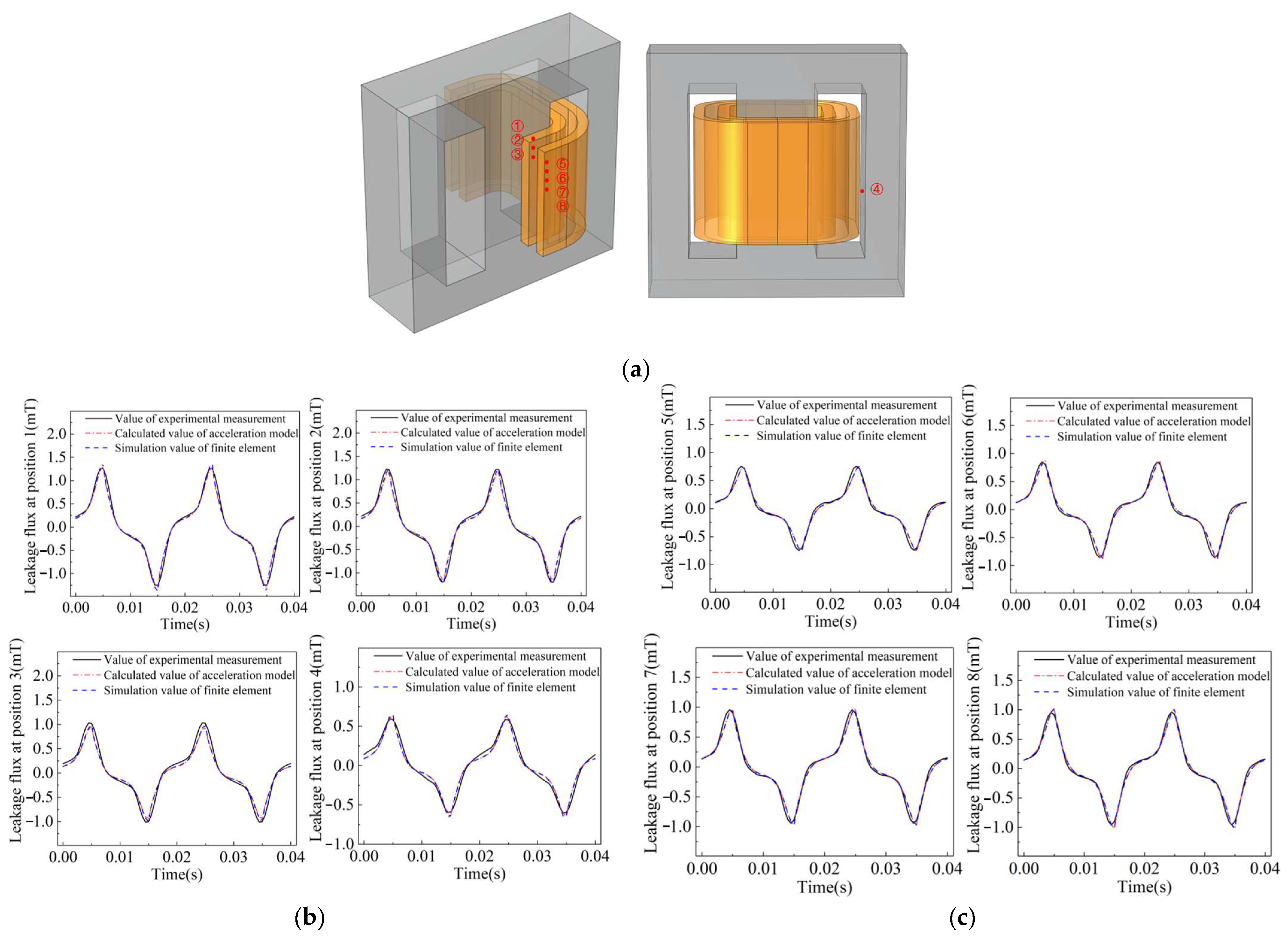
2.2. Construction and Verification of Finite Element Model for Single-Phase Transformer

The geometric and electrical parameters of the test transformer are shown in Table 2.
In order to reduce the computational complexity of the finite element simulation, some factors are ignored based on the symmetry of the transformer, and the finite element model is simplified as follows [26]:
  • Neglecting the influence of structural components such as iron core pull plates and upper and lower clamps on transformers;
  • Neglecting the gaps between transformer winding pads, pressure plates, support bars, and wire cakes;
  • Ignoring the iron-core-laminated structure does not affect calculation accuracy and can reduce computational complexity; therefore, it is considered as a whole for modeling and analysis.
A 3D finite element simulation model of the experimental transformer is established based on the parameters in Table 1 and Table 2, as shown in Figure 3.
An external circuit is built as an external excitation for joint simulation. The external circuit connection is shown in Figure 4, and the expression for the power supply voltage is:
V = 2 U N h sin ( 100 π t + φ )
In this formula, UNh is the effective value of the AC power supply voltage and φ is its initial phase angle.
As shown in Figure 5, the comparison between the voltage and current curves of the primary winding obtained from experiments and simulations at rated voltage verifies the accuracy of the finite element model.
By configuring a transient solver to solve the spatial magnetic field and setting the simulation duration and step size, the magnetic field solution of the test transformer can be completed. Based on this model, changing the parameters can obtain multi-condition finite element simulation data.

3. Sample Data Construction for the Fast Calculation Model of Magnetic Fields

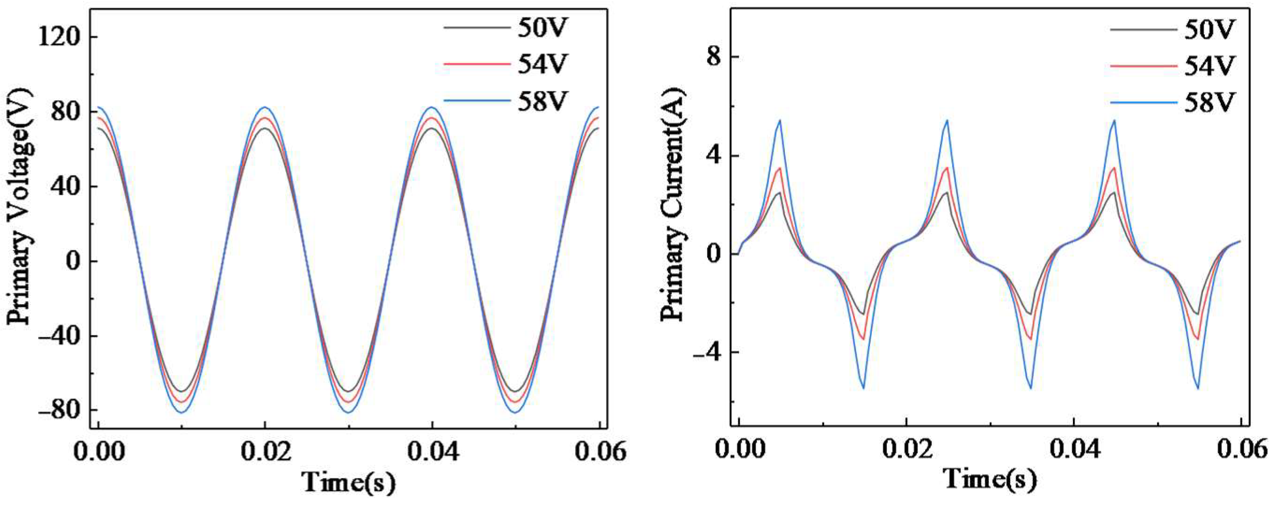
3.1. Multi-Condition Simulation of Single-Phase Transformers

In power grid fault emergencies, transformers may withstand the effect of overvoltage. For example, in the event of a line fault and the action of a single-sided circuit breaker, the reverse power supply of distributed power sources can cause overvoltage at the neutral point of the connected transformer, leading to the saturation of the transformer magnetic circuit and putting it in a nonlinear working state. The transformer is affected by direct current during operation, and the excitation current is superimposed with a DC component. At this time, the iron core is in a saturated abnormal working state, which affects the performance and losses of the transformer. After the transformer is put into operation or the transformer experiences a brief power outage, the instantaneous increase in excitation current leads to magnetic circuit saturation, resulting in transient nonlinear effects that may have a significant impact on the magnetic field distribution and electrical characteristics of the transformer. Therefore, finite element simulation calculations were conducted for these three working conditions.
Considering the insulation and safety performance of transformers, as well as laboratory safety operation regulations, the maximum voltage for the safe operation of test transformers should not exceed 1.1 to 1.2 times the rated voltage of the transformers. Therefore, based on the finite element simulation of transformers under normal operating conditions, the amplitude value Un of the excitation power supply is parameterized and scanned from the rated voltage of 1.0 p.u. (50 V) to 1.3 p.u. (65 V) with a scanning step of 0.02 p.u., and 16 nonlinear magnetic field simulation results of power frequency overvoltage can be obtained. The amplitude of the no-load current of the test transformer is about 2.5 A. When the average current value in one cycle of the test is around 1.35 A, the majority of the current waveform is already above 0 A. Therefore, when parameterizing the DC bias condition based on the finite element simulation of the transformer under normal operating conditions, a current bias Id is added to the excitation power supply for parameterization scanning from 0 A to 2 A, with a scanning step of 0.1 A. The magnetic field simulation results under 20 DC bias conditions can be obtained. In theory, 0° closing is the most severe operating condition for excitation inrush current, while 90° closing is the phenomenon of no excitation inrush current. Therefore, when conducting the parameterized scanning of excitation inrush current conditions based on the finite element simulation of transformers under normal operating conditions, the closing angle of the excitation source is measured. φ is scanned from 0° to 90° with a scanning step of 5°, and magnetic field simulation results under 18 excitation inrush current conditions are obtained.
Based on the supercomputing platform, the finite element simulation results of the magnetic field under the 90 working conditions shown in Table 3 are calculated. The data derived from the simulation results can be used as a source of data for deep learning network training. Below are some simulation results. For power frequency overvoltage conditions, when the power supply increases the voltage beyond the nominal voltage at equal intervals, the transformer core saturates and operates in the nonlinear region. The higher the voltage, the more the corresponding current amplitude increases. For DC bias working conditions, when the average current within a cycle is about the same as the rated current, the waveform will show serious deviation, and the difference in voltage is not significant at this time. For the excitation inrush current condition, there is a significant difference in the first peak value of the excitation current when the initial phase angle of the sine power supply is connected to the circuit changes. When the initial phase angle is 90°, there is no excitation inrush current phenomenon. It can be seen in Figure 6, Figure 7 and Figure 8 that the simulation results conform to the principle analysis and actual objective laws, and can serve as a data source for studying the operating characteristics of experimental transformers.

3.2. Sample Data Construction

Considering that voltage and current are fundamental physical quantities during transformer operation and are easily measurable data, using these two physical quantities as model inputs is practically feasible. Exporting finite element simulation results can be used to construct a data set for training deep learning networks, which includes the time series data U and I of winding port voltage and current, spatial coordinates X, Y, Z, and matrix D, and corresponding magnetic field time series data B, where magnetic field data B can be any direction component or modulus of x, y, or z. A time series matrix for port input voltage and current is constructed as follows:
[ U ,   I ] = [ u 1 , 1 u 2 , 1 u k , 1 i 1 , 1 i 2 , 1 i k , 1 u 1 , 2 u 2 , 2 u k , 2 i 1 , 2 i 2 , 2 i k , 2 u 1 , t u 2 , t u k , t i 1 , t i 2 , t i k , t ]
In this formula, ui, ii (i = 1, 2, …, k) represent the winding voltage and current, k represents the number of windings, and t represents the length of the sequence data.
Considering the significant difference between the main magnetic flux and leakage magnetic flux in space, the spatial region is divided into two parts and a field point matrix is constructed:
D = [ D Z D L ] = [ x Z 1 y Z 1 z Z 1 x Z m y Z m z Z m x L 1 y L 1 z L 1 x L n y L n z L n ]
The magnetic flux density corresponding to the field point as the main flux BZ and leakage flux BL is derived, and the field matrix is constructed:
B = [ B Z B L ] = [ b Z 1 , 1 b Z 1 , 2 b Z 1 , t b Z m , 1 b Z m , 2 b Z m , t b L 1 , 1 b L 1 , 2 b L 1 , t b L n , 1 b L n , 2 b L n , t ]
In this formula, m and n, respectively, represent the number of corresponding coordinate points derived from the main magnetic flux and leakage magnetic flux.

3.3. Data Preprocessing

In the data set constructed in the previous section, time series matrices U and I are used as input data Xraw, and spatial flux matrices BZ and BL are used as output data Yraw.
X raw = [ U ,   I ] = [ x 1 ,   x 2 ,   ,   x t - 1 ,   x t ] T
Y raw = B i = [ y 1 , y 2 , , y t 1 , y t ]   ( i = Z   or   L )
For actual data measured using probes or sensors, the on-site environment may cause random interference. To weaken the impact of noise in the measurement data, median filtering is used to filter the data, as shown in Equation (7). Through filtering, isolated noise points can be eliminated, resulting in data close to the original value.
c i = M e d { d i v , , d i , , d i + v } , i N , v = m 1 2
In this formula, ci is the i-th data point in the filtered sequence data, di is the i-th data point in the prefiltered sequence data, and m is the length of the filtered window.
In order to eliminate the training weight bias caused by the order of magnitude of the features in each dimension, we make it easier for the model to learn the relationships between features, and improve the training effectiveness and generalization performance of the model. This article uses the zero score normalization method to preprocess the raw data. Xraw and Yraw are, respectively, calculated using Equations (8) and (9) to obtain XZ and YZ.
x z = x μ 1 σ 1
y z = y μ 2 σ 2
In this formula, xz and yz are the normalized values, while x and y are the original voltage, current, and magnetic field values, μ1 and μ2, respectively, represent the mean of the input and output sample data; σ1 and σ2, respectively, represent the standard deviation of the input and output sample data.
To ensure that there are sufficient data for learning during the model training process, as well as sufficient data to validate the performance of the model and evaluate its generalization ability on unseen data, the total data sets XZ and YZ are divided into a training set [Xtrain, Ytrain], a testing set [Xtest, Ytest], and a validation set [Xval, Yval] in a 7:2:1 ratio.

4. Training of CNN-LSTM Magnetic Field Fast Calculation Model

This simulation is based on the Python language implementation of the PyTorch framework, with hardware platform settings as follows: (1) CPU: Intel i5-10400 2.90 GHz; (2) GPU:NVIDIA GeForce GTX 1080 Ti 11 G; (3) RAM:16 GB.

4.1. Construction of CNN-LSTM Network Model

For single-phase dual-winding transformers, k = 2 in Equation (2), m = 1291 in Equation (4), and n = 17,202. Each finite element simulation result exports 0.04 s of data (with a time interval of 0.5 ms) for a total of 81 time steps. Based on the parameterized scanning results, t = 11,097 in the input and output matrices.
Based on the voltage and current of the transformer winding, the magnetic field value of the space is quickly calculated. Due to the nonlinear characteristics of the transformer core, the voltage, current, and spatial magnetic field are nonlinear correspondences. Therefore, the CNN network is selected. The three physical quantities have a back-to-back dependence in time. Therefore, the LSTM network is selected. Considering the significant differences in the distribution of main and leakage magnetic flux, this section constructed a dual-branch deep learning model using the CNN and LSTM. The training network structure is shown in Figure 9. The size of the input data set is 11,097 × 4, the size of the output data set is 11,097 × 18,493, and the input characteristic quantity is the voltage and current of the primary and secondary side windings. The training set contains 7768 data points, and the test set contains 2219 data points. The training set is used for model learning and parameter adjustment, and the test set is used to verify the performance of the model, thus ensuring the generalization ability and robustness of the model. The normalized voltage and current matrix XZ is input into the training branches of the main flux and leakage flux, respectively. At the same time, it is mapped to high-dimensional spatial features through a CNN network. The output matrix of the CNN is transformed and directly input into the LSTM network to extract its temporal dependencies. Finally, it is separated by a fully connected layer, decoded, and linearly mapped to output spatial main flux and leakage flux Y1 and Y2. The two results are concatenated to obtain the complete calculation result of the accelerated simulation model. The specific methods are as follows.
The input voltage and current matrix Xraw defined in Equation (5) is normalized by Equation (8) to obtain the input matrix XZ. As shown in Equation (10), the data xt−1 at time t−1 of XZ is convolved to extract features. The convolved outputs are weighted and biased separately, and the sum is added to obtain ut. Then, the output xt of the fully connected layer is obtained through the activation function ReLU.
x t = f ( w t x t 1 + b t )
In this formula, f represents the activation function, wt is the weight coefficient, and bt is the bias.
The output xt of CNN and the hidden state ht−1 of the LSTM network at time t−1 are used as inputs for the LSTM network at time t. The LSTM processing input data includes three steps. Firstly, there is the forget gate, where the input data is weighted and biased before activating the function σ to obtain the forgotten information ft, expressed in Equation (11), where the output of the activation function is any value between [0, 1].
f t = σ ( w f [ h t 1 , x t ] + b f )
Next is the input gate, where the input data is calculated using new weighted biases and then passed through a separate activation function σ and tanh layer to obtain the intermediate input it and intermediate cell state C t ˜ . The calculation formula is as follows:
i t = σ ( W i [ h t 1 , x t ] + b i )
C t ˜ = tanh ( W c [ h t 1 , x t ] + b c )
In this formula, Wi and Wc respectively correspond to ht−1 and xt to the weight matrix of the input gate activation function σ and tanh, where bi and bc are the corresponding biases.
The forgetting information ft is multiplied by the corresponding element of the cell state Ct−1 at time t−1, and the intermediate input it is multiplied by the corresponding element of the intermediate cell state C t ˜ . After adding the two, the cell state Ct at time t is obtained. The calculation formula is as follows:
C t = f t C t 1 + i t C t ˜
In this formula, is the Hadamard product operator, which represents the operation of multiplying the corresponding elements of two matrices.
Finally, the output gate is used, and after the input is subjected to another weighted bias calculation, the output information ot of the output gate is obtained via the activation function σ, and the expression is calculated as in Equation (15). The cell state Ct at time t is processed by the tanh layer and multiplied by the corresponding element ot to obtain the output ht of the hidden layer at time t. The calculation formula is shown in Equation (16).
o t = σ ( W o [ h t 1 , x t ] + b o )
h t = o t tanh ( C t )
In this formula, Wo is the weight of ht−1 and xt to the output gate activation function σ, and bo is the corresponding bias.
The structural parameters of the CNN-LSTM are determined based on the network structure and data characteristics, as shown in Table 4.

4.2. Training of CNN-LSTM Network Model

This study uses mean absolute error (MAE), mean square error (MSE), and R-Square (R2) as evaluation indicators to evaluate the accuracy of the model. The expressions for each indicator are as follows:
MAE = 1 n i = 1 n | y ^ i y i |
MSE = 1 n i = 1 n ( y ^ i y i ) 2
R 2 = 1 i = 1 n ( y i y ^ i ) 2 i = 1 n ( y i y ¯ ) 2
In the formula, n is the number of samples in the test set derived from finite element simulation, y ^ i is the i-th value calculated by the model, y i is the i-th true value of the test set, which is the finite element calculation value, and y ¯ is the average of the i-th finite element calculation value of the test set.
Batch size refers to the number of samples used during each iteration of training. A larger batch size can accelerate the training process, but it will occupy more memory. The learning rate is a hyperparameter used to control the step size or speed of model parameter updates. A higher learning rate can lead to unstable training processes and may not converge. The optimizer is an algorithm used to adjust model parameters to minimize the loss function, which affects the convergence speed and performance of the model. Therefore, the selection of batch size, learning rate, and optimizer affects the convergence time and computational efficiency of deep learning networks. During network training, three parameters are tested with different values, and the mean square error is used as the loss function during the training process. By comparing the loss functions, the batch size and learning rate were determined to be 64 and 0.01, respectively. When using the optimizer Adam, the loss function value was minimized, which means the error was minimized.
Based on the MSE, the loss function diagram is drawn, as is shown in Figure 10. In the first 500 iterations, the loss value rapidly decreases, and after 2000 iterations, it tends to stabilize, with the loss value stabilizing at around 0.01. The trained model takes approximately 0.04 s to calculate a single output time, achieving a fast calculation effect.

4.3. LSTM/CNN/MLP Network Comparison

The grid search method is used to obtain the optimal hyperparameter combination of different networks. The proposed model is compared with the calculation indexes of the LSTM, CNN, and multi-layer perceptron (MLP). The performance is shown in Figure 11. The MSE of the proposed model is the smallest, and R2 is the closest to 1. Therefore, the CNN-LSTM model proposed in this paper has a better comprehensive effect.
Under the condition that the learning rate, the iteration period, and the optimizer are fixed, the scale of the training data set is adjusted by changing the scanning step size. Five cases are set, as shown in Table 5. Δu, ΔI, and Δφ are the parametric scanning step sizes of power frequency overvoltage, DC bias, and inrush current finite element simulation, respectively. The larger the step size, the smaller the data set size.
For the transformer model in this paper, different deep learning networks are used to train the goodness of fit R2 of different data set sizes. As shown in Figure 12, in the case of more data (such as Table 5 number 1), the R2 values of all networks are above 0.9, and different networks have a different sensitivity to the change of data set size. In the case of small data set size, this method still has certain advantages. Taking R2 above 0.95 as the requirement of network calculation accuracy, parametric scanning according to the step size number 2 in Table 5 can meet the requirements. Transformers of different sizes only affect the number of points in the magnetic field data, and the same step size configuration can be used to construct the data set.

5. Comparison and Verification of Fast Calculation Models for Magnetic Fields

5.1. Methodology

The construction steps of the fast calculation model of magnetic fields are as follows:
(1) Construction of the finite element model: After obtaining the geometric parameters and electrical parameters of the transformer, the geometric model is established in the finite element simulation software according to the parameters. The external circuit excitation is set, the transient solver is configured, and the finite element simulation model of the three-dimensional magnetic field of the transformer under normal working conditions is output.
(2) Parameterized scanning of the supercomputing platform to obtain data: Based on the finite element simulation model in the previous step, the voltage amplitude, DC component, and closing phase angle set by the external circuit in the model are parameterized by the supercomputing platform to obtain a large number of simulation results under nonlinear conditions. The time series winding voltage and current are derived as the input data set and the magnetic field point cloud data as the target data set.
(3) Accelerate the training of the calculation model: The data set in the previous step is preprocessed and divided as the data basis for accelerating the training of the calculation model. The dual-branch training network is constructed by combining the CNN and LSTM to determine the appropriate number of iterations, batch data size, learning rate, and other network hyperparameters. The mapping relationship between the main and leakage flux and the voltage and current is trained, and the model file containing the network parameters is output.
(4) Application of the accelerated calculation model: The model file output is called from the previous step, the spatial magnetic field output corresponding to the specified winding voltage and current input is calculated, and the error between the output value of the model and the finite element calculation value or the measured value on the time and space scale are compared.

5.2. Comparison Validation

When constructing the sample data, the data set is divided into a training set, a testing set, and a validation set. In the previous section, a single-phase transformer magnetic field acceleration calculation model was trained based on the training set sample learning. In this section, the trained magnetic field fast calculation model file is called, the space point magnetic field data corresponding to the input data in the verification set are output, and the magnetic field value output by the magnetic field acceleration calculation model is compared with the magnetic field value measured in the test and the results of the finite element simulation. The finite element simulation results are the label samples in the test set, so as to further analyze and verify the accuracy of the output results of the magnetic field acceleration calculation model.
In the experiment, the radial and axial components of the magnetic field at multiple points were measured. The magnetic field data from 8 measurement points, as shown in Figure 13a, were compared with the output values of the acceleration calculation model and finite element simulation values. Among them, the radial magnetic field components were compared between the measurement points near the side column and between the windings, numbered ①–④. The axial magnetic field components were compared between the measurement points parallel to the winding core column on the outer side of the winding and four measurement points on the winding axis, numbered ⑤–⑧. The variation curves over time and the measured waveforms were compared, as shown in Figure 13b,c. The root mean square errors of positions ①–④ were 0.0822 mT, 0.1038 mT, and 0.0979 mT, respectively. The ratio of T and 0.0514 mT to the peak value is within 10%. The root mean square errors of positions ⑤–⑧ are 0.0496 mT, 0.0468 mT, 0.0538 mT, and 0.0500 T, respectively, and the ratio to the peak value is within 5%. The results indicate that the fit of the three curves is high for different positions and directional components, and the overall error of the axial component of the magnetic field is smaller than that of the radial component.

6. Conclusions

This paper proposes a fast calculation model for transformer spatial magnetic fields based on finite element simulation and the CNN-LSTM. The model designs a dual output structure based on the difference between the main and leakage magnetic fluxes, and extracts the mapping relationship between voltage and current and spatial magnetic field based on CNN multi-layer mapping encoding. Then, the bidirectional LSTM is used to extract the temporal dependence relationship between the electric field and magnetic field. Finally, after decoding, the linear mapping outputs the spatial main and leakage magnetic fluxes calculated by the model. Through matrix fusion, the complete spatial magnetic field can be obtained. Through simulation analysis, algorithm comparison, and experimental verification, the following conclusions have been drawn:
  • This model designs a dual-branch spatial dynamic magnetic field fast calculation model based on the CNN-LSTM, which divides the spatial magnetic field solving task into two subproblems, avoiding the fitting bias caused by the difference in main and leakage magnetic flux, and has certain interpretability and accuracy.
  • This model is based on a multi-condition finite element simulation that takes into account the nonlinear characteristics of the iron core, with a focus on learning and mapping the behavior of the nonlinear effects of the iron core on magnetic field distribution, in order to achieve a more efficient and accurate fast calculation of magnetic field distribution within the framework of digital twins.
  • The calculated output time of the trained model at a single time step is about 0.04 s, which greatly shortens the time compared to finite element simulation. The calculated values of the model showed good consistency with the experimental measurements at different locations and time periods.

Author Contributions

The authors gratefully acknowledge the contributions as following: X.Z. performed the experiments; Q.P. wrote the manuscript; D.Z. analyzed the data; Z.H. wrote the code; R.G. and D.C. read and edited the manuscript. All authors have read and agreed to the published version of the manuscript.

Funding

This research was funded by Electric Power Research Institute of Yunnan Power Grid Co., Ltd. Finite Element-Based Computational Modeling of Physical Quantities of Transformers and Disconnectors with Training Database Construction (YNKJXM20220008).

Data Availability Statement

All data generated or used during the study are reasonably available from the corresponding author.

Acknowledgments

Project Supported by Electric Power Research Institute of Yunnan Power Grid Co., Ltd. Finite Element-Based Computational Modeling of Physical Quantities of Transformers and Disconnectors with Training Database Construction (YNKJXM20220008).

Conflicts of Interest

The authors declare no conflicts of interest.

References

  1. Arraño-Vargas, F.; Konstantinou, G. Modular Design and Real-Time Simulators toward Power System Digital Twins Implementation. IEEE Trans. Ind. Inform. 2023, 19, 52–61. [Google Scholar] [CrossRef]
  2. Yang, F.; Hao, H.; Wang, P.; Jiang, H.; Xia, Y.; Luo, A.; Liao, R. Development status of multi-physical field numerical calculation for power equipment. High Volt. Eng. 2023, 49, 2348–2364. [Google Scholar]
  3. Moutis, P.; Alizadeh-Mousavi, O. Digital Twin of Distribution Power Transformer for Real-Time Monitoring of Medium Voltage From Low Voltage Measurements. IEEE Trans. Power Deliv. 2021, 36, 1952–1963. [Google Scholar] [CrossRef]
  4. Deng, X.; Zhu, H.; Yan, K.; Zhang, Z.; Liu, S. Research on transformer magnetic balance protection based on optical fiber leakage magnetic field measurement. Trans. China Electrotech. Soc. 2024, 39, 628–642. [Google Scholar]
  5. Zhou, Y.; Wang, X. Online monitoring method of transformer winding deformation based on magnetic field measurement. Electr. Meas. Instrum. 2017, 54, 58–63+87. [Google Scholar]
  6. Zhang, C.; Zhou, L.; Li, W.; Gao, S.; Wang, D. Calculation method of energy-saving coil core loss considering boundary flux density classification. High Volt. Eng. 2023, 49, 3940–3948. [Google Scholar]
  7. Stulov, A.; Tikhonov, A.; Snitko, I. Fundamentals of Artificial Intelligence in Power Transformers Smart Design. In Proceedings of the 2020 International Ural Conference On Electrical Power Engineering (UralCon), Chelyabinsk, Russia, 22–24 September 2020. [Google Scholar]
  8. Pan, Q.; Ma, W.; Zhao, Z.; Kang, J. Development and application of magnetic field measurement methods. Trans. China Electrotech. Soc. 2005, 3, 7–13. [Google Scholar]
  9. Wan, B. Research on the Detection Method of Electromagnetic Wave Magnetic Field Component at the Joint of Transformer Partial Discharge Oil Tank. Master’s Thesis, North China Electric Power University (Beijing), Beijing, China, 2023. [Google Scholar]
  10. Taher, A.; Sudhoff, S.; Pekarek, S. Calculation of a Tape-Wound Transformer Leakage Inductance Using the MEC Model. IEEE Trans. Energy Convers. 2015, 30, 541–549. [Google Scholar] [CrossRef]
  11. Zhao, Y.; Dai, Y.; Zhuang, J.; Cai, G.; Chen, Z.; Liu, X. Optimization method of insulation material performance parameters of medium frequency transformer based on thermo-solid coupling. Trans. China Electrotech. Soc. 2023, 38, 1051–1063. [Google Scholar]
  12. Yan, C.; Hao, Z.; Zhang, B.; Zheng, T. Modeling and Simulation of Deformation Rupture of Power Transformer Tank. Trans. China Electrotech. Soc. 2016, 31, 180–187. [Google Scholar]
  13. ANSYS. Ansys Twin Builder. Available online: https://www.ansys.com/zh-cn/products/digital-twin/ansys-twin-builder (accessed on 10 May 2024).
  14. Zhang, C.; Liu, D.; Gao, C.; Liu, Y.; Liu, G. Three-dimensional magnetic field reduction model and loss analysis of 110 kV oil-immersed transformer based on Twin Builder. High Volt. Eng. 2024, 50, 941–951. [Google Scholar]
  15. COMSOL. COMSOL Multiphysics®6.2 Release Highlights. Available online: https://cn.comsol.com/release/6.2 (accessed on 10 May 2024).
  16. Liu, Y.; Li, Y.; Li, H.; Fan, X. Local hot spot detection of transformer winding based on Brillouin optical time domain peak edge analysis. Trans. China Electrotech. Soc. 2024, 39, 3486–3498. [Google Scholar]
  17. Taheri, A.A.; Abdali, A.; Rabiee, A. A Novel Model for Thermal Behavior Prediction of Oil-Immersed Distribution Transformers With Consideration of Solar Radiation. IEEE Trans. Power Deliv. 2019, 34, 1634–1646. [Google Scholar] [CrossRef]
  18. Liu, G.; Hao, S.; Hu, W.; Liu, Y.; Li, L. Calculation method of transient temperature rise of oil-immersed transformer winding based on SCAS time matching algorithm. Trans. China Electrotech. Soc. 2024, 1–14. [Google Scholar]
  19. Deng, X.; Wu, W.; Yang, M.; Zhu, H. Research on transformer winding deformation diagnosis based on leakage magnetic field and deep belief network. Transformer 2021, 58, 42–48. [Google Scholar]
  20. Deng, X.; Yan, K.; Zhu, H.; Zhang, Z. Early fault protection based on transformer winding circuit-leakage magnetic field multi-state analytical model. Grid Technol. 2023, 47, 3808–3821. [Google Scholar]
  21. Khan, A.; Ghorbanian, V. Lowther. Deep Learning for Magnetic Field Estimation. IEEE Trans. Magn. 2019, 55, 7202304. [Google Scholar] [CrossRef]
  22. Fotis, G.; Vita, V.; Ekonomou, L. Machine Learning Techniques for the Prediction of the Magnetic and Electric Field of Electrostatic Discharges. Electronics 2022, 11, 1858. [Google Scholar] [CrossRef]
  23. Zhang, Y.; Zhao, Z.; Xu, B.; Sun, H.; Huang, X. Research on fast calculation method of electromagnetic field based on U-net convolutional neural network. Trans. China Electrotech. Soc. 2024, 39, 2730–2742. [Google Scholar]
  24. Li, P.; Hu, G. Transformer fault diagnosis method based on data-enhanced one-dimensional improved convolutional neural network. Grid Technol. 2023, 47, 2957–2967. [Google Scholar]
  25. Fan, Z.; Du, J. Prediction of dissolved gas volume fraction in transformer oil based on correlation variational mode decomposition and CNN-LSTM. High Volt. Eng. 2024, 50, 263–273. [Google Scholar]
  26. Pan, C.; An, J.; Liu, C.; Cai, G.; Sun, Z.; Luo, Y. Multi-field coupling analysis and suppression of noise characteristics of transformer bias effect. Trans. China Electrotech. Soc. 2023, 38, 5077–5088. [Google Scholar]
Figure 1. Test platform.
Energies 17 03913 g001
Figure 2. Parameter identification of J-A model.
Energies 17 03913 g002
Figure 3. Test transformer for finite element simulation model.
Energies 17 03913 g003
Figure 4. External circuit connection chart.
Energies 17 03913 g004
Figure 5. Comparison of voltage and current curves between test and simulation.
Energies 17 03913 g005
Figure 6. Finite element simulation results (power frequency overvoltage).
Energies 17 03913 g006
Figure 7. Finite element simulation results (DC bias).
Energies 17 03913 g007
Figure 8. Finite element simulation results (inrush current).
Energies 17 03913 g008aEnergies 17 03913 g008b
Figure 9. Structure of CNN-LSTM network.
Energies 17 03913 g009
Figure 10. Training and testing loss function curve.
Energies 17 03913 g010
Figure 11. Comparison curve of calculation indexes of different algorithms.
Energies 17 03913 g011
Figure 12. Curve of the R2 of different networks with the size of the data sets.
Energies 17 03913 g012
Figure 13. The comparison curve between the calculated and actual measured value of magnetic flux leakage: (a) Location of magnetic field measurement points. (b) Radial magnetic field measurement value and acceleration simulation calculation value. (c) Axial magnetic field measurement value and acceleration simulation calculation value.
Energies 17 03913 g013
Table 1. Parameters of J-A model.
ParametersValue
Saturation intensity Ms (A/m)1.2166 × 106
Nailing loss k (A/m)68.626
Reversibility of magnetization c0.0307
Interdomain coupling α3.027 × 10⁻⁴
Domain wall density a (A/m)134.7
Table 2. Test-transformer-related parameters.
ParametersValueParametersValue
Nominal capacity/VA50Turns ratio55:55
Nominal voltage/V50Iron core materialDQ151-φ0.35
Width of center leg/mm60Window height/mm124
Iron core thickness/mm60Window width/mm36
Width of sideward leg/mm30Winding height/mm90
Table 3. Summary of simulation conditions in the database.
Working ConditionLoad SituationParameterized ScanningNumber of Operating Conditions (Group)
Power frequency overvoltageSecondary side unloadUN: 1.0–1.3 p.u.
Scanning step size 0.02 p.u.
16
Secondary side load16
DC biasSecondary side unloadIs: 2 A–50 A,
Scanning step size 2 A
20
Secondary side load20
Inrush currentSecondary side unloadφ: 0°–120°, Scanning step size 5°18
Total operating conditions90
Table 4. CNN-LSTM training structure parameter table of spatial magnetic flux.
Training Layer TypeParameter StructureTraining Layer TypeParameter Structure
Convolutional layer weights(32, 1, 3)LSTM layer bias2(256)
Convolutional bias(32)Fully connected layer 1 weight(1291, 1024)
LSTM layer weight 1(256, 32)Fully connected layer 1 bias(1291)
LSTM layer weight 2(256, 64)Fully connected layer 2 weight(17,202, 1024)
LSTM layer bias 1(256)Fully connected layer 2 bias(17,202)
Table 5. Different data set sizes.
Number12345
Δu/p.u.0.020.040.060.080.1
ΔI/A246810
Δφ510152025
Disclaimer/Publisher’s Note: The statements, opinions and data contained in all publications are solely those of the individual author(s) and contributor(s) and not of MDPI and/or the editor(s). MDPI and/or the editor(s) disclaim responsibility for any injury to people or property resulting from any ideas, methods, instructions or products referred to in the content.

