Abstract
This paper presents a fast focusing inversion algorithm of magnetic data based on the conjugate gradient method, which can be used to describe the underground target geologic body efficiently and clearly. The proposed method realizes an effect similar to matrix compression by changing the computation order, calculating the inner product of vectors and equivalent expansion of expressions. Model tests show that this strategy successfully reduces the computation time of a single iteration of the conjugate gradient method, so the three-dimensional magnetic data inversion is realized under a certain number of iterations. In this paper, the detailed calculation steps of the proposed inversion method are given, and the effectiveness and high efficiency of the proposed fast focusing inversion method are verified by three theoretical model tests and a set of measured data. Finally, the fast focus inversion algorithm is applied to the magnetic data of Gonghe Basin, Qinghai Province, to describe the spatial distribution range of deep hot dry rock, which provides a direction for the continuous exploration of geothermal resources in this area.
1. Introduction
The magnetic method is one of the commonly used geophysical methods. Magnetic exploration is used to detect the target of underground addresses by studying the magnetic anomaly of different degrees caused by magnetic differences. The magnetic exploration method [1] plays an important role in ore exploration and oil and gas exploration. For example, for metal minerals, magnetic exploration methods can be used to directly search for ore (such as chromite, magnetite, etc.) according to their high magnetic characteristics. In the geological exploration of oil and gas fields and coal fields, most sedimentary rocks are almost non-magnetic, while underlying igneous rocks and bedrock are usually weakly magnetic. The depth of the bedrock is determined by magnetic exploration, and thus the thickness of the sediment is determined. Because basement relief can produce tectonic relief in overlying sedimentary rocks, which is conducive to oil and gas accumulation, the determination of bedrock relief can provide useful data and guidance for oil and gas exploration.
Magnetic data inversion refers to the quantitative calculation of magnetic distribution in underground space using either linear or nonlinear algorithms. This calculation helps to obtain the shape, burial depth and magnetic susceptibility distribution information of the anomalous body, which provides an essential reference for the subsequent geological interpretation. Nonlinear methods, such as genetic algorithms, Monte Carlo algorithms, and simulated annealing algorithms [2,3], are effective in reducing the possibility of falling into local extreme situations during the search process, but they usually have a significant computational problem when dealing with small data. On the other hand, linear inversion methods, including the conjugate gradient method, fastest descent method, damped least square method, Newton method, and others, are more mature and widely used after decades of development [4,5,6].
In 1975, Green [7] utilized the Backus–Gilbert method and incorporated prior geological information into the inversion process to accomplish two-dimensional linear gravity inversion. Tikhonov and Arsenin [8] utilized the regularization technique to constrain the physical property parameters, incorporating a minimum norm constraint to ensure a stable solution for potential field data inversion. In the process of inversion, due to the “skin effect”, the inversion results of field data tend to the surface, which makes it difficult to reflect the real physical property distribution of the body. Li and Oldenburg [9] incorporated the model weighting matrix into the objective function of gravity inversion, effectively addressing the “skin effect” issue. This inversion theory has good stability, but it is prone to a “trailing phenomenon” at the bottom of the anomalic body, and the horizontal and depth resolution are not high; that is, the inversion results diverge and do not focus.
For the problem of relatively divergent inversion results, Last and Kubik [10] first introduced the model minimum volume constraint in gravity inversion in 1983, and they obtained the inversion effect with clear boundaries and focused parameter distribution. This constraint method is essentially approximated to the L0 norm constraint of the model. Since then, the method based on minimum volume constraint has been widely used in geophysical inversion, and on this basis, a variety of high-resolution inversion methods have been developed. In 1999, Portniaguine and Zhdanov [11] built upon this idea and introduced the minimum gradient support function as part of the compact inversion process. This method, known as focusing inversion, generates anomalous body distributions with sharp boundaries. In 2002, Portniaguine and Zhdanov [12] proposed to use the reweighted conjugate gradient algorithm to solve the focusing inversion results in the weighted density parameter space. In 2004, Zhdanov et al. [13] applied the focused inversion method to the inversion calculation of gravity and gravity gradient data. In 2009, Zhdanov [14] derived a new focusing inversion formula and applied it to gravity data inversion. Focusing inversion technology can restore gravity or magnetic anomaly objects with clear boundaries, which plays an important role in current potential field data inversion methods.
The three-dimensional focusing inversion of magnetic data is a technique that can provide valuable information about the distribution of magnetic susceptibility in the Earth’s subsurface. This information can be used as a reference for future geological studies. Due to the significance of focusing inversion in potential field data processing, this paper establishes a magnetic data target inversion function based on the focusing constraint. The conjugate gradient method can solve linear equations efficiently and quickly, and it has been widely applied in geophysical inversion, such as seismic tomography, magnetotelluric inversion, and resistivity imaging [15]. This method has several advantages, such as requiring less memory, being suitable for large-scale calculation, having fast convergence, and being stable [15]. Therefore, this paper uses the conjugate gradient method to solve the magnetic data inversion problem.
With the improvement of acquisition accuracy and exploration ability, it is more and more important to use a high-precision magnetic survey for the fine interpretation of geological targets. However, when the amount of data increases significantly, the conjugate gradient algorithm will face problems of large memory consumption and long computation time during the iterative solution process [4,16,17,18,19,20,21]. To achieve large data inversion, it is crucial to use more efficient optimization techniques [22,23,24,25] or compression methods [26,27,28]. This paper proposes a conjugate gradient optimization algorithm to solve the problem of low computational efficiency when the amount of data increases. The main objective is to reduce the use of computer memory, improve operation efficiency, and achieve fast inversion by avoiding storing and processing large matrices in the iterative process.
The method proposed in this paper is applied to the Qiabuqia area in Gonghe, Qinghai Province, so as to provide a reference for the detection of hot dry rock. Firstly, the geological background of Gonghe area in Qinghai Province and the research status of hot dry rock detection are introduced. Secondly, in the theoretical part, the calculation process of the fast focusing inversion algorithm is introduced in detail. Next, the inversion efficiency of the proposed algorithm is verified through three sets of theoretical model tests in the data testing part, and then the algorithm is applied to the republican ground magnetic data to describe the distribution range of hot dry rock. Finally, in the discussion section, the time advantage of the fast algorithm and the reference information provided by the actual data inversion results for the detection of hot dry rocks are analyzed.
2. Geological Setting
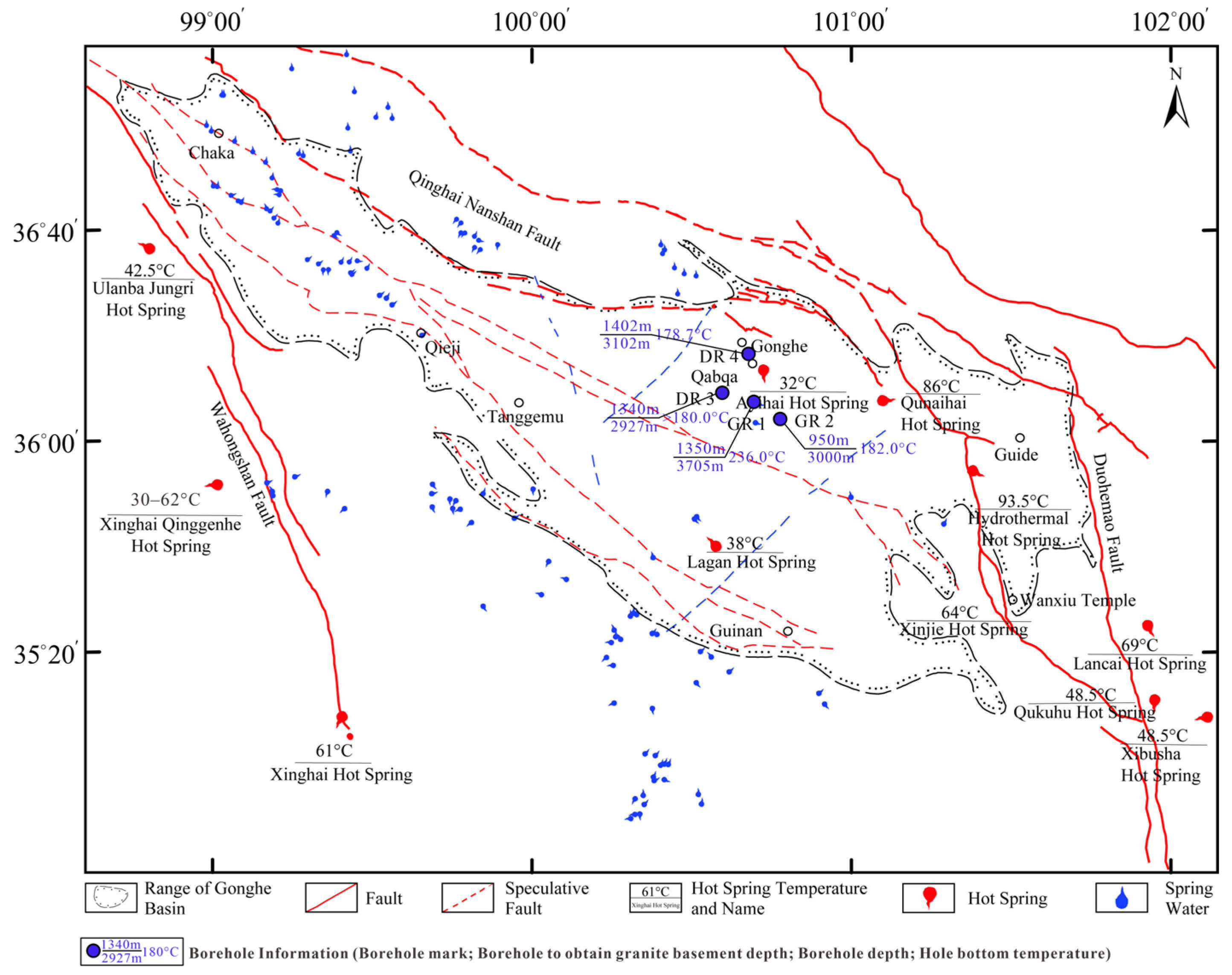
The Qiabuqia area in Gonghe, Qinghai Province (Figure 1) is a significant region in China with promising potential for the exploration and development of hot dry rock geothermal resources. Situated in the northeastern region of the Qinghai–Tibet Plateau, commonly referred to as the “roof of the world”, this area is characterized by a rhomboid-shaped fault basin that formed during the Cenozoic period. To the north of the basin, the Zongwulong Mountain–Qinghai Nanshan fault zone connects it with the Qilian orogenic belt. To the south, it borders the Songpan–Ganzi block via the Animaqing suture zone. The Duohemao Fault on the eastern side overlooks the Wahongshan Fault on the western side [29,30].
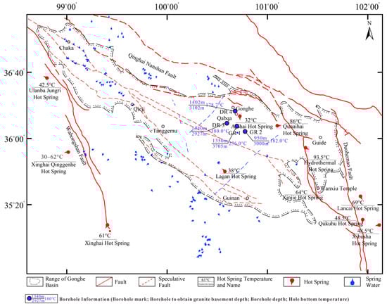
Figure 1.
Distribution of main faults, boreholes and hot springs in Gonghe Basin and its surrounding areas (revised from Feng et al. [31]).
In terms of tectonic evolution, the Gonghe Basin has gone through two stages: rift depression from the Early Paleozoic to the Late Paleozoic and intracontinental tectonic evolution since the Mesozoic [32]. The Indosinian period marked a critical juncture in the tectonic evolution of the Gonghe Basin, characterized by the westward subduction of the Gonghe Valley, which ultimately closed beneath the Qaidam block [33]. Concurrently, the basin experienced intense magmatic intrusion, resulting in the exposure of numerous intrusive rocks in the surrounding regions. The current tectonic framework was ultimately established by the superimposition of the western basin’s uplift during the Yanshanian epoch and the differential uplift of the northeastern margin of the Qinghai–Tibet Plateau during the Himalayan epoch [34].
The heat flow within the basin is notably high, and the average geothermal gradient of the basement granite exceeds 5 °C/100 m, resulting in distinct thermal anomalies. According to early geophysical data, the Gonghe Basin comprises five secondary tectonic units: Tanggemu Depression, Guide Depression, Guinan Depression, Qijia Uplift, and Yellow River Uplift [35]. The Qiabuqia geothermal region is situated at the transitional slope between the Tanggemu Depression and the Yellow River Uplift. The geothermal energy in this region is of the conductive type, with its heat source originating from deep within the earth. The temperature profiles from the wells exhibit linear characteristics [36].
Within and around the basin, there are six hot springs with temperatures exceeding 60 °C with the highest reaching 93.5 °C at Zhacangsi Hot Springs. These hot springs are densely distributed along the fault zone [30]. There are two types of geothermal resources in basins: fault structure and sedimentary basin. The former is mostly located near the fault zone at the edge of the basin and transfers heat through thermal convection, while the latter is generally located inside the basin and transfers heat through thermal conduction [29,35].
Table 1 presents the fundamental characteristics of the thermal anomaly hot dry rock temperature measurement borehole as documented by Zhang et al. [37] in the Gonghe Qiabuqia area. Their findings indicate that boreholes DR3, DR4, and GR1 in the Chabcha area all exhibit subsurface temperatures exceeding 150 °C at depths around 2700 m. In 2017, China [38] successfully drilled a high-temperature hot dry rock mass with a temperature of 236 °C at a depth of 3705 m underground in the area, providing further evidence for the exceptional abundance of geothermal resources in the Gonghe Basin.

Table 1.
Basic information of borehole for temperature measurement of hot dry rock in thermal anomaly area of Chabcha area (revised from Zhang et al. [37]).
The relationship between rock magnetism and temperature is complicated, but the general trend is that the magnetic susceptibility increases with increasing temperature. Therefore, regions where hot dry rocks occur usually exhibit relatively high magnetic characteristics. Xue et al. [30] investigated the geophysical characteristics of the subsurface hot dry rock mass in the Gonghe Basin by integrating gravity, magnetic, and electrical exploration results with physical property parameters in the area, employing both forward and inverse analysis methods. Their research findings indicate that the hot dry rock mass exhibits characteristics of low density, high resistance, and medium-weakness magnetism, which are geophysical indicators for hot dry rock exploration.
Zhang et al. [39] conducted an analysis of the magnetic parameters for 505 rock samples collected from the orogenic belt surrounding the Gonghe Basin. Their findings indicate that rocks of varying ages and lithologies exhibit distinct magnetic properties: (1) in Proterozoic strata, the rock magnetism is predominantly within the range of (14.2–25.4) × 10−5 SI, indicating relatively weak magnetic properties; (2) IndoChiese granite is widely distributed with a magnetic susceptibility value ranging from (0.3–2500) × 10−5 SI and varying magnetic strength; (3) the shallow metamorphic sedimentary strata widely distributed around the Gonghe Basin exhibit a magnetic susceptibility ranging (18.3–31.7) × 10−5 SI and possess weak magnetic properties, whereas the remaining formation rocks display either weakly magnetic or non-magnetic characteristics. The magnetic anomalies associated with paleoproterozoic metamorphic rocks and pre-Indochinese granites are concentrated in the Qilian orogenic belt to the northeast of the Gonghe Basin. Anomalies related to alteration zones and mineralization are primarily distributed in the Nanshan area of Qinghai province, which is located to the northwest of the Gonghe Basin. Magnetic anomalies resulting from IndoChinese concealed medium acid granites are widely spread throughout the Gonghe Basin. Through drilling verification, it has been confirmed that the Qiabuqia hidden IndoChinese intermediate acidic granite body with high magnetic anomaly characteristics has been confirmed to be a hidden dry hot rock mass. Consequently, buried IndoChinese magnetic medium acid granites within the Gonghe Basin can be considered as potential exploration targets for hot dry rocks.
Therefore, through magnetic data inversion, this paper predicts the distribution area of underground hot dry rock in Gonghe area according to the high magnetic characteristics.
3. Magnetic Data Inversion Theory
3.1. Optimization of the Magnetic Data Inversion Results
Magnetic inversion is a method used to determine the underground structure and magnetic properties of anomalous bodies based on magnetic data obtained on the observation surface. The mathematical equation represented by the linear inversion problem is shown in Formula (1):
where is the observed data vector, is the parameter vector of the model to be found, and is the forward sensitivity matrix. M represents the dimension of the observed data vector, and N represents the dimension of the model parameter vector, which is usually M << N.
The solution of Formula (1) is usually translated into the Tikhonov regularization optimal problem shown in Formula (2):
where is the regularization parameter, is the actual observed magnetic data, and is the prior model. is a data weighting matrix [10] used to improve the magnetic data affected by ambient noise. is a depth-weighted matrix [10], which is used to improve the depth resolution of magnetic data inversion results. is a focusing operator matrix [8,11] used to produce a compact model result. , , and are diagonal matrices, and their definitions are given in Formulas (3)–(5):
This paper adopts the reweighting algorithm [10] to solve the problem in Formula (2), which is specifically shown in Formulas (6)–(9):
where is the weighted domain sensitivity matrix, is the weighted domain model parameter vector, and is the weighted domain observed data vector.
3.2. Traditional Conjugate Gradient Algorithm for Magnetic Data Based on Focusing Constraints
The conjugate gradient method is a method between the fastest descent method and Newton method. It not only overcomes the slow convergence of the fastest descent method but also avoids the disadvantages of the Newton method, which need to store and calculate the Hesse matrix and its inverse. The conjugate gradient method is one of the most useful methods to solve large linear equations, which can obtain the desired solution with a certain number of iterations only by using the first derivative information [40].
The conjugate gradient method is employed to determine the optimal solution of Formula (6). The first derivative of the objective function with respect to the model weighting parameter is given in Formulas (10)–(12):
To update the regularization parameter , an adaptive method [10] is applied. The calculation rule of α with respect to the iteration number k is given in Formula (13):
Because the magnetic susceptibility of rocks in the Earth’s crust is often within a specific range and region, the latter can be further reduced according to the known geological conditions. Therefore, setting the maximum and minimum values of the physical property parameters as the upper and lower limits is a very simple and effective method. In this paper, the inversion parameters are controlled in a more reasonable range by Formula (14).
In summary, the traditional magnetic data inversion algorithm based on focusing constraints is shown in Algorithm 1.
| Algorithm 1 The traditional magnetic data focusing inversion algorithm |
| Start: k = 0; m0 = 0.001; ; f0 = Rm0 − r; d0 = f0 |
| Repeat |
| k = k + 1 |
| If is sufficiently small, then exit loop |
| End repeat |
3.3. Magnetic Data Acceleration Conjugate Gradient Algorithm Based on Focusing Constraints
The conjugate gradient method has a fast convergence rate, so it is difficult to compress the number of iterations to achieve the purpose of fast calculation. In this paper, the idea of fast calculation is to reduce the calculation time of each iteration so as to realize the fast inversion of magnetic data. The core process of the conjugate gradient method in one iteration calculation is as follows: (1) calculate the first derivative; (2) calculate the search direction; and (3) calculate the search step size. Therefore, the essence of reducing the time of each iteration is to improve the time efficiency of the above three processes:
- (a).
- Improvements to the calculation efficiency of the first derivative: From Formulas (10)–(12), it is evident that the first derivative comprises three components, the first of which is derived by multiplying the three variables , and . The product of these three variables is two calculation orders: or . The essence of the first order of computation is that the computer first obtains the large matrix and then multiplies the matrix with the long vector . The essence of the second order is that the computer first obtains the short vector , and then performs matrix multiplication with the small matrix . Note that the terms “large matrix”, “small matrix”, “long vector”, and “short vector” are relative terms. In this paper, the time cost of calculating the first derivative of the two computing sequences is tested: under the grid background of 32 × 32 × 16, the time of calculating the first derivative of the former is about 5.35 s, and the time of calculating the first derivative of the latter is about 0.14 s. The experiment shows that the order of calculation obviously has an important effect on the speed of derivative calculation. The traditional method is to use the first calculation order; this paper suggests to use the second calculation order when dealing with large-scale data.
- (b).
- Improvements to search direction computing efficiency: When calculating the search direction of the conjugate gradient method, three long vectors , and need to be stored in advance. The function of is to give the inner product value of the gradient in the previous iteration when calculating the current iteration. However, this is entirely unnecessary. This paper proposes pre-calculating the inner product of the gradient vector obtained from each iteration and passing the resulting gradient inner product value to the next iteration instead of the gradient vector. In this way, only two long vectors and can be stored in each iteration, thus reducing the memory consumption of the computer and improving the operation and storage efficiency.
- (c).
- Improvements to search step size calculation efficiency: When calculating the search step size in the traditional conjugate gradient method, the denominator part needs to use a large matrix of stored in advance. However, the computer consumes too much memory to store large matrices, so this article does not recommend storing large matrices in advance. In this paper, it is suggested that the denominator is partially equivalent to be expanded into a linear combination of a small matrix and vector in order to avoid the situation of storing a large matrix of in the calculation process. This practice can reduce the memory consumption, thus improving the computing efficiency of the computer. The improved calculation details are given in Formula (15):
By changing the calculation order, inner product prediction and equivalent expansion, the memory consumption of the first-order derivative, search direction and search step length of each iteration is reduced, so as to reduce the calculation time of each iteration and realize fast magnetic data inversion. The improved algorithm is shown in Algorithm 2.
| Algorithm 2 Fast focusing inversion algorithm for magnetic data |
| Start: k = 0; m0 = 0.001; ; ; d0 = f0 |
| Repeat |
| k = k + 1 |
| If is sufficiently small, then exit loop |
| End repeat |
4. Data Testing
4.1. Synthetic Data Testing
Three classical magnetic anomaly models are established to demonstrate the high efficiency of the fast focusing inversion algorithm. (1) Model I: two magnetic anomaly prismatic models with relative depth; (2) Model II: a magnetic susceptibility model of an inclined plate; (3) Model III: a combination model of multiple magnetic anomaly prisms. The same coordinate system is used for all three models, with the X-axis pointing north, the Y-axis pointing east, and the Z-axis pointing down. The magnetic anomaly data of Model I and Model II were measured on a 32 × 32 grid in the x and y directions, and the magnetic anomaly data of Model III were measured on a 40 × 40 grid in the x and y directions. The sampling interval of the three models was 100 m. To make the simulation data more authentic, 2% Gaussian random noise is added to the synthesized magnetic anomaly data. The background field intensity of each model is 50,000 nT, and the degree of polarization of the background field varies from model to model.
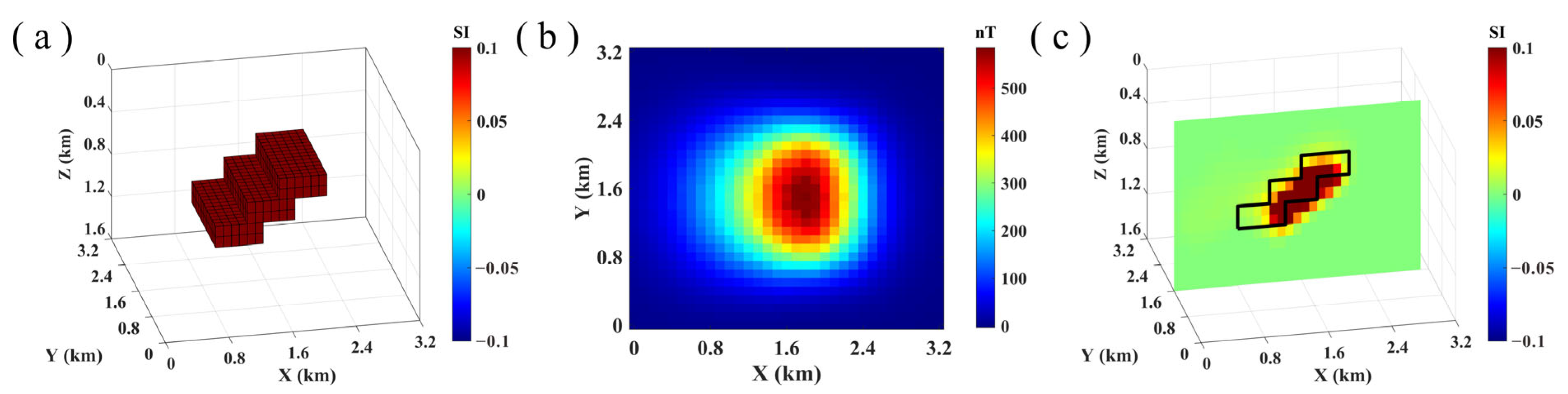
Figure 2a shows a three-dimensional view of Model I, which is composed of two magnetic anomaly prisms with a relative burial depth of 0.5 km × 1 km × 0.4 km, which both have a remanent magnetic susceptibility of 0.1 SI. The buried depth at the top of the shallow prisms is 0.4 km. The depth at the top of the deep prism is 0.6 km. The background field intensity is 50,000 nT, with an inclination (I) and declination (D) of 90° and 0°, respectively. Figure 2b shows the noise observation data of the model at the surface. The fast algorithm and traditional algorithm are used to invert the simulation data with noise. The inversion parameters were set as follows: the maximum depth of inversion is 1.6 km, and the model network used is composed of 0.1 km × 0.1 km × 0.1 km cubic units, so the number of units in the model grid is 32 × 32 × 16. The magnetic susceptibility constraint range is [0 0.1] SI; the upper limit for the number of iterations is set to k = 100; and the cutoff error is set to . Inversion stops after 51 iterations. The total iteration time of the fast algorithm is 3.63 s, so the single iteration time is 0.07 s. The full iteration time of the traditional algorithm is 283.51 s, and the single iteration time is 5.56 s. The depth cross-section was taken at y = 1.6 km to show the inversion results of Model I, as shown in Figure 2c. In the latter, the black border represents the actual boundary of the model body established, and it can be seen that the inversion results indeed show the position of the model.
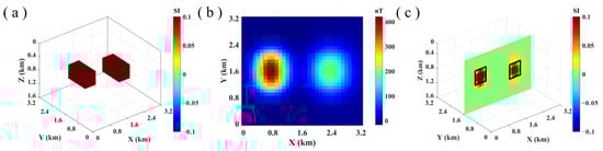
Figure 2.
(a) Model I. (b) Model I data with noise. (c) Inversion results along y = 1.6 km.
Model II represents an inclined plate’s three-dimensional magnetic susceptibility model, as shown in Figure 3a. The direction of the plate is from y1 = 0.8 km to y2 = 2.2 km. It has an upward trend from x1 = 0.8 km to x2 = 2.2 km with a north–south direction. The top depth of the board is 0.8 km. The remanent magnetic susceptibility in the plate is uniformly distributed and equal to 0.1 SI. The background field intensity is 50,000 nT, and its inclination (I) and declination (D) are 50° and 10°, respectively. Figure 3b displays the noise observation data of the model at the surface. The data in Figure 3b were inverted using the acceleration and traditional algorithms, and the inversion parameters were the same as those applied in Model I. The inversion process stops after 71 iterations. The total iteration time of the fast algorithm is 4.98 s, and the single iteration time is 0.07 s. The full iteration time of the traditional algorithm is 400.05 s, and the single iteration time is 5.63 s. To display the inversion results of Model II, the cross-section is taken at y = 1.6 km, as shown in Figure 3c. The black border represents the established actual boundary of the model body. The magnetic susceptibility distribution obtained by inversion is concentrated in the plate’s real position, providing reliable tilt information.

Figure 3.
(a) Model II. (b) Model II data with noise. (c) Inversion results along y = 1.6 km.
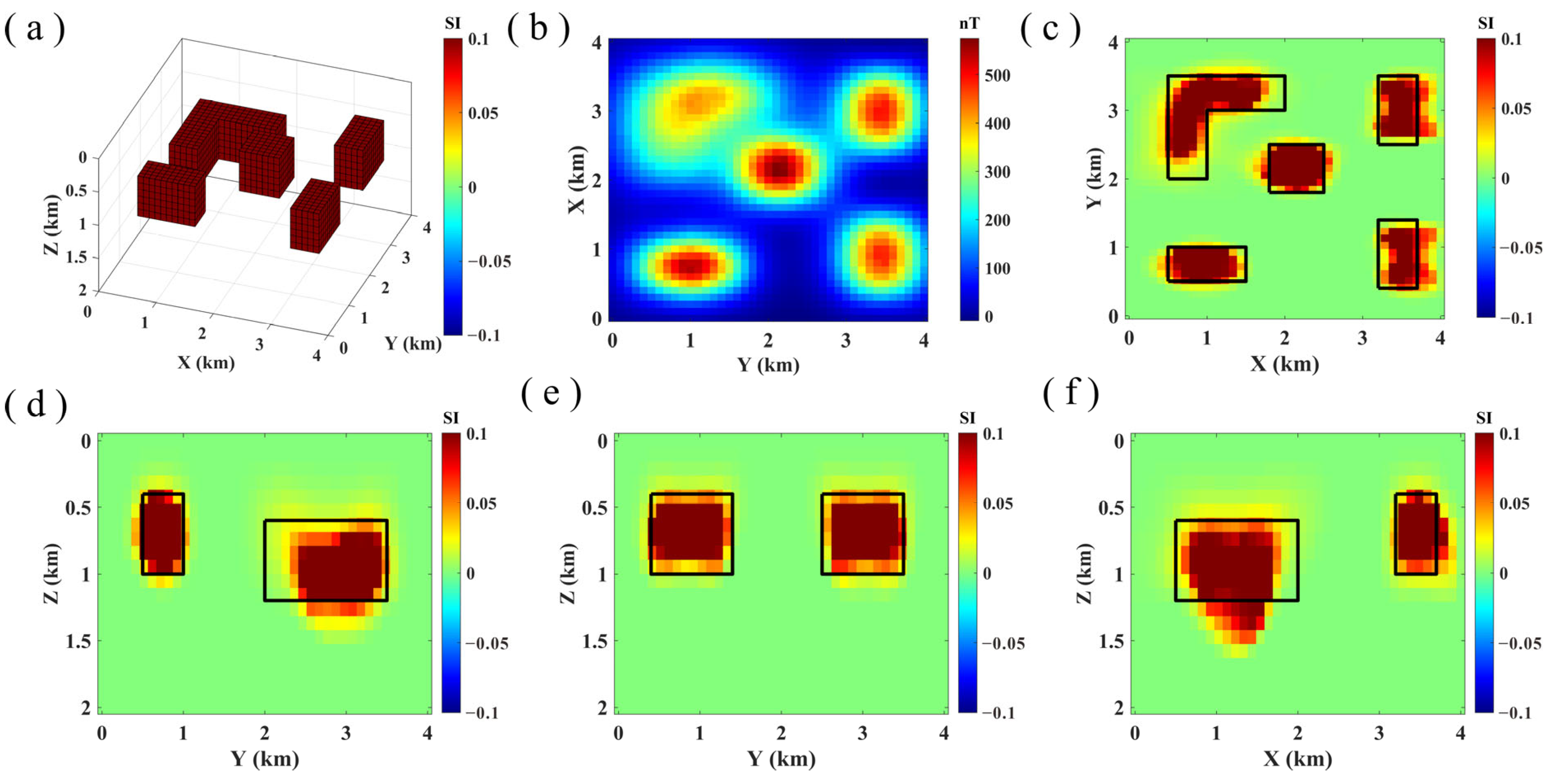
The three-dimensional view of Model III is given by Figure 4a, which is a combined model of multiple magnetic anomaly prisms to further test the inversion performance of the algorithm in complex cases. Model III has a total of six prisms, two of which are put together to form an L-shaped object. The specific parameters of the six prisms are shown in Table 2. The remanent susceptibility of all prisms is evenly distributed and is equal to 0.1 SI. The background field intensity is 50,000 nT, I = 60°, D = −10°. Figure 4b depicts the noise observation data of the model at the surface. The acceleration algorithm and traditional algorithm were used to invert the data in Figure 3b, and the inversion parameters were set as follows: maximum depth of inversion is 2.0 km, and the model network used is composed of 0.1 km × 0.1 km × 0.1 km cubic units, so the number of units of the model grid is 40 × 40 × 20. The magnetic susceptibility constraint range is [0 0.1] SI; the upper limit for the number of iterations is set to k = 200; the cut-off error is set to . The inversion process stops after 188 iterations. The total and single iteration time of the acceleration algorithm is 39.77 s and 0.21 s, respectively. The total and single iteration time of the traditional algorithm is 7711.46 s and 41.02 s, respectively. Three deep cross-sections and one cross-section are performed (Figure 4c–f), and the true boundary of the model body is represented by a black border. The results reveal that the distribution of magnetic susceptibility is in good agreement with the black box given.

Figure 4.
(a) Model III. (b) Model III data with noise. (c) Inversion results along z = 0.8 km. (d) Inversion results along x = 0.8 km. (e) Inversion results along x = 3.5 km. (f) Inversion results along y = 3.2 km.
Table 2.
Parameters of Model III.
After conducting the three sets of experiments, it is evident that the acceleration algorithm proposed in this paper produces reliable magnetic data inversion results and is more efficient compared to the traditional algorithm. Specifically, when the data scale of inversion is 32 × 32 × 16, the acceleration algorithm takes around 0.07 s for a single iteration, while the traditional algorithm takes around 5.6 s for a single iteration, and the acceleration ratio is 80 times. When the data scale of inversion is expanded to 40 × 40 × 20, the single iteration time of the accelerated and the traditional algorithm is around 0.2 s and 40 s, respectively, and the acceleration ratio is about 200 times.
4.2. Real Data Testing
The ground magnetic data of Gonghe Basin used in this paper were collected by the Institute of Geological Survey of Jilin University in 2016. Due to the small measurement range of surface magnetic survey data, the main geological targets for 3D physical property inversion based on the separated magnetic data are the cover layer and heat reservoir. There are developed geothermal wells in the central and eastern regions of the survey area, and proven thermal storage in the central and western regions, but the connectivity of the thermal storage is unknown. The main purpose of magnetic inversion is to study the distribution and connectivity of the two heat reservoirs and provide information for further development.
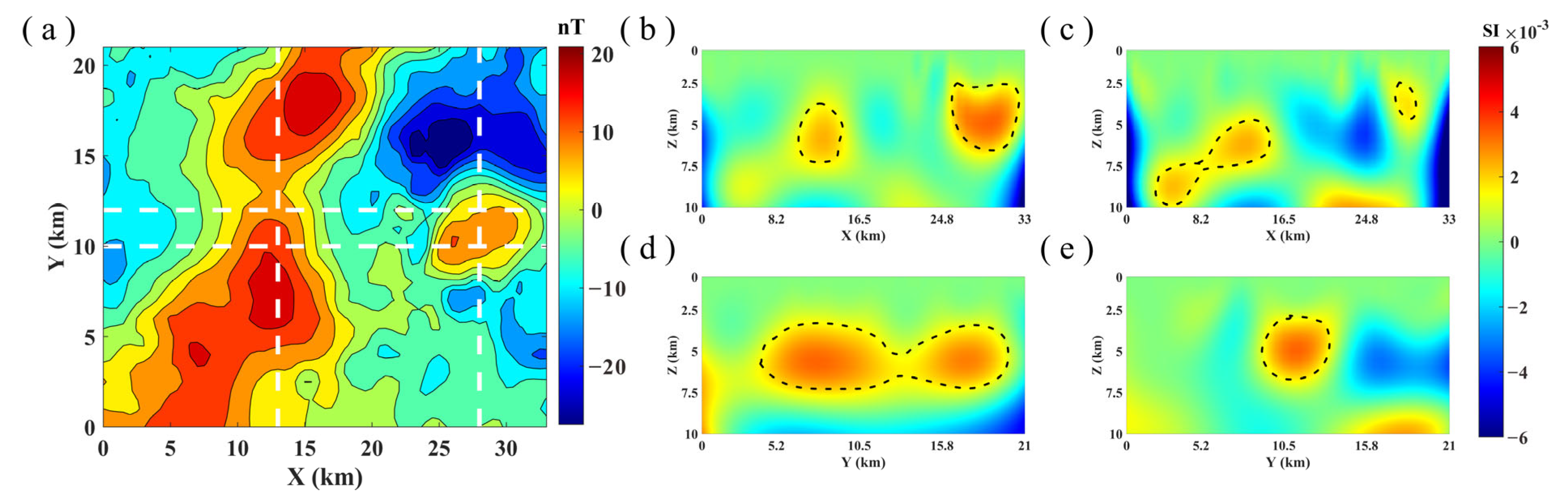
After technical processing such as early daily variation correction, normal field correction, polarization, and anomaly separation, the local magnetic anomaly data of the ground in the Qiabuqia area of the Gonghe Basin are shown in Figure 5a, and the entire measurement area is 33 km × 21 km. The inversion depth was set to 10 km, and the underground space of the data acquisition area is divided into 40 × 40 × 20 structural cube units with the size of each unit being 825 m × 525 m × 500 m. This paper chooses the four important cross-sections that show focusing inversion results of magnetic susceptibility distribution, as shown in Figure 5b–e. In Figure 5, the white dashed line marks the surface locations of the four cross-sections, and the black dashed line delineates the possible distribution of heat storage. According to the three-dimensional inversion results of magnetic data, there are obvious weak magnetic, high magnetic and low magnetic layers in the measurement area. The shallow weak magnetic layer is abnormally small, which corresponds to the relatively low magnetic characteristics of the cap layer to the reservoir. The heat storage in the middle layer shows high magnetic characteristics, while the deep surrounding rock shows low magnetic characteristics. The connectivity of the heat storage is excellent, and the conditions of the cover layer are also good.
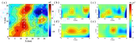
Figure 5.
(a) Gonghe ground magnetic data. (b) Inversion results along y = 10 km. (c) Inversion results along y = 13 km. (d) Inversion results along x = 12 km. (e) Inversion results along x = 28 km (the white dashed lines indicate the positions of the four slices, while the black dashed lines mark potential locations for delineated hot dry rocks).
According to the three-dimensional inversion results of magnetic data, the hot dry rock reservoir area shows high magnetic characteristics, with a depth of 2.5~7 km, which is in good correspondence with the known drilling data such as GR1 and GR2 in Qiabuqia town in the central and eastern part of the survey area. The inversion results also show that the subsurface high magnetic anomalies are mainly distributed in the eastern and western regions, and the thermal reservoirs in the central and western regions have good spatial connectivity with the hot dry rock reservoirs in the central and eastern regions. Among them, the mideast high magnetic anomaly is small in scale and shallower in burial. The high magnetic anomalies in the midwest are larger in scale and buried relatively deep. The midwest regions are the next areas to focus on exploration and detailed investigation.
5. Discussions
5.1. Computational Time Advantage Analysis
In the synthetic data test part, the performance of the fast focusing inversion algorithm is demonstrated by three sets of models, and the results show that the algorithm can obtain reliable magnetic data inversion results. The model tests of the three groups all recorded the time cost of the fast algorithm and the traditional algorithm in processing the same magnetic data, and it can be seen that the fast focusing inversion algorithm is more efficient and practical than the traditional algorithm.
In order to better highlight the time efficiency of the fast algorithm, this paper uses the magnetic data obtained from the synthetic model III for three-dimensional magnetic susceptibility inversion with grid numbers of 20 × 20 × 20, 40 × 40 × 20, 50 × 50 × 20, 80 × 80 × 20. In Table 3, the single iteration time of inversion for the two algorithms under different scale data is recorded. According to the records in Table 3, it can be seen that on the same computer, the traditional algorithm can no longer calculate the grid number after 50 × 50 × 20, but the fast algorithm still realizes the efficient magnetic data inversion.
Table 3.
Comparison of calculation time of single iteration for Model III with different grid numbers.
5.2. Analysis of Inversion Results and Location of Hot Dry Rock Target Area
According to the three-dimensional inversion results of local magnetic anomalies in the Gonghe Qiabuqia area, there are obvious weak magnetic, high magnetic and low magnetic structures in the measurement area. Among them, the weak magnetic part is a shallow layer from near the surface to a depth of about 3 km underground, corresponding to the Quaternary loose or weak diagenetic strata. The quaternary sedimentary layer corresponding to the weak magnetosphere has the characteristics of discontinuous distribution and obvious thickness change in the section, showing a trend of thinning from west to east on the whole, and it is the thermal insulation layer of heat storage. The central high-magnetic part is distributed in the stratum with a thickness of about 4 km, which is the main area for the distribution of hot dry rocks, and the overall distribution shows the characteristics of deep burial in the west and shallow burial in the east. A large continuous low magnetic section corresponds to the bottom granite basement. Since the temperature change is mainly manifested as the demagnetization of magnetic minerals and negative magnetic or weak magnetic anomalies, it is speculated that the extensive low magnetic characteristics of granite basement may be related to the demagnetization of magnetic minerals caused by deep thermal factors.
Table 4 shows the statistical information of hot dry rock exploration boreholes distributed in the middle of the eastern part of the survey area. It can be seen from the table that the four boreholes explored high-temperature granite at depths of 2.5–3.7 km. On the other hand, the inversion results of this paper show that hot dry rocks with high magnetic properties are mainly distributed in the middle east and western regions with subsurface depths of about 2.5–7 km. Three cross-sections with borehole information are selected to further prove the validity of the inversion results. According to the magnetic susceptibility inversion results in Figure 6a–c, it is analyzed that the underground heat storage area is within the range of 2.5–6 km. This prediction is consistent with the drilling exploration results presented in Table 4, suggesting that this paper provides practical and effective reference for inferring the thermal storage location based on the inversion results of magnetic data. Simultaneously, taking into account the inversion results depicted in Figure 5, it can be inferred that there may exist hot dry rocks at a depth of 4–8 km in the western region. Therefore, this paper suggests that the next area of focus for exploration and detailed investigation should be the western region.
Table 4.
Hot dry rock exploration borehole statistics in Chabucia area, Gonghe Basin (revised from Zhang et al. [38]).
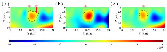
Figure 6.
(a) The inversion result of the slice containing GR1 and DR4 indicates that x = 26 km. (b) The inversion result of the slice containing GR2 indicates that x = 30 km. (c) The inversion result of the slice containing DR3 indicates that x = 24 km (the solid red lines in the figure indicate the location and length of the corresponding holes, while the black dashed lines mark potential locations for delineated hot dry rocks).
6. Conclusions
This paper presents a fast 3D inversion algorithm for magnetic data based on the focusing constraint. This method can successfully reduce the time consumption of the conjugate gradient method in one iteration by changing the calculation order, calculating the inner product of the gradient vector and equivalent expansion. Therefore, in the case of the same number of iterations, the fast algorithm brings considerable time benefits compared with the traditional algorithm. In the data test, satisfactory 3D magnetic susceptibility distribution imaging results are obtained. Through a comparative analysis of calculation time, it can be seen that the new algorithm is fast, efficient and expandable. The calculation time of the fast algorithm in one iteration is usually 50 times faster than that of the traditional algorithm, so the new algorithm is efficient and practical in large-scale magnetic data inversion.
Author Contributions
Conceptualization, W.D. and H.J.; methodology; writing—review and editing, N.J. and Y.L.; result interpretation; project administration, H.J. and W.Z.; writing—review and editing; supervision, Z.Z. and S.Z.; project administration. All authors have read and agreed to the published version of the manuscript.
Funding
This research was funded by a grant from the Ph.D. Programs Foundation of Ministry of Gan Dong College (No. 122000801) and Science Foundation of Jiang-Xi Educational Committee (No. 191612).
Data Availability Statement
The original contributions presented in the study are included in the article, further inquiries can be directed to the corresponding author.
Conflicts of Interest
The authors declare no conflicts of interest.
References
- Nabighian, M.N.; Hansen, R.O.; Lafehr, T.R.; Li, Y.; Peirce, J.W.; Phillips, J.D.; Ruder, M.E. The historical development of the magnetic method in exploration. Geophysics 2005, 70, 33ND–61ND. [Google Scholar] [CrossRef]
- Boschetti, F.; Dentith, M.; List, R. Inversion of potential field data by genetic algorithms. Geophys. Prospect. 1997, 45, 461–478. [Google Scholar] [CrossRef]
- Guan, Z.-N.; Hou, J.-S.; Huang, L.-P.; Yao, C.-L. Inversion of gravity and magnetic anomalies using pseduo-BP neural network method and its application. Chin. J. Geophys. 1998, 41, 242–251. [Google Scholar]
- Pilkington, M. 3-D magnetic imaging using conjugate gradients. Geophysics 1997, 62, 1132–1142. [Google Scholar] [CrossRef]
- Li, Y.; Melo, A.; Martinez, C.; Sun, J. Geology differentiation: A new frontier in quantitative geophysical interpretation in mineral exploration. Lead. Edge 2019, 38, 60–66. [Google Scholar] [CrossRef]
- Zhdanov, M.S.; Alfouzan, F.; Cox, L.H.; Alotaibi, A.M.; Alyousif, M.M.; Sunwall, D.; Endo, M. Large-Scale 3D Modeling and Inversion of Multiphysics Airborne Geophysical Data: A Case Study from the Arabian Shield, Saudi Arabia. Minerals 2018, 8, 271. [Google Scholar] [CrossRef]
- Green, W.R. Inversion of Gravity Profiles by Use of a Backus-Gilbert Approach. Geophysics 1975, 40, 763–772. [Google Scholar] [CrossRef]
- Tikhonov, A.N.; Arsenin, V.Y. Solusions of Ill-Posed Problems; John Wiley and Sons, Inc.: Hoboken, NJ, USA, 1977. [Google Scholar]
- Li, Y.; Oldenburg, D.W. 3-D inversion of gravity data. Geophysics 1998, 63, 109–119. [Google Scholar] [CrossRef]
- Last, B.J.; Kubik, K. Compact gravity inversion. Geophysics 1983, 48, 713–721. [Google Scholar] [CrossRef]
- Portniaguine, O.; Zhdanov, M.S. Focusing geophysical inversion images. Geophysics 1999, 64, 874–887. [Google Scholar] [CrossRef]
- Portniaguine, O.; Zhdanov, M.S. 3-D magnetic inversion with data compression and image focusing. Geophysics 2002, 67, 1532–1541. [Google Scholar] [CrossRef]
- Zhdanov, M.S.; Ellis, R.; Mukherjee, S. Three-dimensional regularized focusing inversion of gravity gradient tensor component data. Geophysics 2004, 69, 925–937. [Google Scholar] [CrossRef]
- Zhdanov, M.S. New advances in regulariaed inversion of gravity and electromagnetic data. Geophys. Prospect. 2009, 57, 463–478. [Google Scholar] [CrossRef]
- Liu, T.Y. New Method for Data Processing of Potential Field Exploration; Science Press: Beijing, China, 2007; pp. 88–113. [Google Scholar]
- Canning, F.X.; School, J.F. Diagonal preconditioners for the EFIE using a wavelet basis. IEEE Trans. Antennas Propag. 1996, 44, 1239–1246. [Google Scholar] [CrossRef]
- Chen, R.S.; Yung, E.K.N.; Chan, C.H.; Wang, D.X.; Fang, D.G. Application of the SSOR preconditioned CG algorithm to the vector fem for 3D full-wave analysis of electromagnetic-field boundary-value problems. IEEE Trans. Microw. Theory Tech. 2002, 50, 1165–1172. [Google Scholar] [CrossRef]
- Moorkamp, M.; Jegen, M.; Roberts, A.; Hobbs, R. Massively parallel forward modeling of scalar and tensor gravimetry data. Comput. Geosci. 2010, 36, 680–686. [Google Scholar] [CrossRef]
- Cuma, M.; Zhdanov, M.S. Massively parallel regularized 3D inversion of potential fields on CPUs and GPUs. Comput. Geosci. 2014, 62, 80–87. [Google Scholar] [CrossRef]
- Hou, Z.L.; Wei, X.H.; Huang, D.N.; Sun, X. Full tensor gravity gradiometry data inversion: Performance Geophysics analysis of parallel computing algorithms. Appl. Geophys. 2015, 12, 292–302. [Google Scholar] [CrossRef]
- Wang, T.H.; Huang, D.N.; Ma, G.Q.; Meng, Z.H.; Li, Y. Improved preconditioned conjugate gradient algorithm and application in 3D inversion of gravity-gradiometry data. Appl. Geophys. 2017, 14, 301–313. [Google Scholar] [CrossRef]
- Hou, Z.L.; Wei, J.K.; Mao, T.X.; Zheng, Y.J.; Ding, Y.C. 3D inversion of vertical gravity gradient with multiple graphics processing units based on matrix compression. Geophysics 2022, 87, 67–80. [Google Scholar] [CrossRef]
- Zhou, S.; Jia, H.F.; Lin, T.; Zeng, Z.F.; Yu, P.; Jiao, J. An accelerated algorithm for 3D inversion of gravity data based on improved conjugate gradient method. Appl. Sci. 2022, 13, 10265. [Google Scholar] [CrossRef]
- Qin, P.B.; Huang, D.N.; Yuan, Y.; Geng, M.X.; Liu, J. Integrated gravity and gravity gradient 3D inversion using the non-linear conjugate gradient. J. Appl. Geophys. 2016, 126, 52–73. [Google Scholar] [CrossRef]
- Cuma, M.; Zhdanov, M.S. Large-scale 3D inversion of potential field data. Geophys. Prospect. 2012, 60, 1186–1199. [Google Scholar] [CrossRef]
- Meng, Z.H.; Xu, X.C.; Huang, D.N. Three-dimensional gravity inversion based on sparse recovery iteration using approximate zero norm. Appl. Geophys. 2019, 15, 524–535. [Google Scholar] [CrossRef]
- Martin, R.; Monteiller, V.; Komatitsch, D.; Perrouty, S.; Jessell, M.; Bonvalot, S.; Lindsay, M. Gravity inversion using wavelet-based compression on parallel hybrid CPU/GPU systems: Application to southwest Ghana. Geophys. J. Int. 2013, 195, 1594–1619. [Google Scholar] [CrossRef]
- Sun, S.Y.; Yin, C.C.; Gao, X.H.; Liu, Y.H.; Ren, X.Y. Gravity compressed sensing forward modeling and multiscale gravity inversion based on wavelet transform. Appl. Geophys. 2018, 15, 342–352. [Google Scholar] [CrossRef]
- Sun, Z.X.; Li, B.X.; Wang, Z.L. Exploration of the possibility of hot dry rock occurring in the Qinghai Gonghe Basin. Hydrogeol. Eng. Geol. 2011, 38, 119–124. (In Chinese) [Google Scholar]
- Xue, J.Q.; Gan, B.; Li, B.X. Geological-geophysical characteristics of enhanced geothermal systems (Hot Dry Rocks) in Gonghe-Guige Basin. Geophys. Geochem. Explor. 2013, 37, 34–41. (In Chinese) [Google Scholar]
- Feng, Y.F.; Zhang, X.X.; Zhang, B.; Liu, J.T.; Wang, Y.G.; Jia, D.L.; Hao, L.H.; Kong, Z.Y. The geothermal formation mechanism in the Gonghe Basin: Discussion and analysis from the geological background. China Geol. 2018, 1, 331–345. [Google Scholar] [CrossRef]
- Chen, P.; Zhou, Y.-L.; Jian, Q.-H.; Wang, Z.; Da, L. Zircon U-Pb dating and geochemistry of clastic sedimentary rocks in the Gonghe-Huashixia Area, Qinghai Province and their geological implications. Earth Sci. Front. 2009, 16, 161–174. (In Chinese) [Google Scholar]
- Zhang, G.W.; Guo, A.L.; Yao, A.P. Western Qinling-Songpan continental tectonic node in China’s continental tectonics. Earth Sci. Front. 2004, 11, 23–32. (In Chinese) [Google Scholar]
- Li, R.B.; Pei, X.Z.; Yang, S.H.; Wang, W.F.; Wei, L.Y.; Sun, Y.; Li, F.; Liu, M.N.; Zhao, C.C.; Li, Z.C.; et al. LA-ICP-MS Zircon age of metamorphism rocks in the Rouqigang Area of western Gonghe basin: Maxinum depositional ages of protoliths and provenance feature. Acta Geol. Sin. 2016, 90, 93–114. (In Chinese) [Google Scholar]
- Zhao, Z. The exploitation and characteristics of the thermal reservior of the Qiabuqia geothermal field in the Qinghai Gonghe basin. Ground Water 2013, 35, 8–10. (In Chinese) [Google Scholar]
- Wenping, X.; Rui, L.; Shengsheng, Z.; Jinshou, Z.; Piaoluo, Y.; Shanshan, Z. Progress in hot dry rock exploration and a discussion on development tectnology in the Gonghe Basin of Qinghai. Pet. Drill. Tech. 2020, 48, 77–84. [Google Scholar]
- Zhang, C.; Zhang, S.; Li, S.; Jia, X.; Jiang, G.; Gao, P.; Wang, Y.; Hu, S. Geothermal characteristics of the Qiabuqia geothermal area in the Gonghe Basin, northeastern Tibetan Plateau. Chin. J. Geophys. 2018, 61, 4545–4557. [Google Scholar]
- Senqi, Z.H.N.; Weide, Y.A.; Dunpeng, L.I.; Xiaofeng, J.I.; Shengsheng, Z.H.N.; Shengtao, L.I.; Lei, F.U.; Haidong, W.U.; Zhaofa, Z.E.G.; Zhiwei, L.I.; et al. Characteristics of geothermal geology of the Qiabuqia HDR in Gonghe Basin, Qinghai Province. Geol. China 2018, 45, 1087–1102. [Google Scholar]
- Zhang, S.Q.; Fu, L.; Zhang, Y.; Song, J.; Wang, F.C.; Huang, J.H.; Jia, X.F.; Li, S.T.; Zhang, L.Y.; Feng, Q.; et al. Delineation of hot dry rock exploration target area in the Gonghe Basin based on high-precision aeromagnetic data. Nat. Gas Ind. 2020, 40, 156–169. [Google Scholar]
- Scales, J.A. Tomographic inversion via the conjugate gradient methods. Geophysics 1987, 52, 179–185. [Google Scholar] [CrossRef]


Disclaimer/Publisher’s Note: The statements, opinions and data contained in all publications are solely those of the individual author(s) and contributor(s) and not of MDPI and/or the editor(s). MDPI and/or the editor(s) disclaim responsibility for any injury to people or property resulting from any ideas, methods, instructions or products referred to in the content. |
© 2024 by the authors. Licensee MDPI, Basel, Switzerland. This article is an open access article distributed under the terms and conditions of the Creative Commons Attribution (CC BY) license (https://creativecommons.org/licenses/by/4.0/).