Abstract
Chiller fault diagnosis plays a crucial role in optimizing energy efficiency within heating, ventilation, and air conditioning (HVAC) systems. The non-stationary nature of chiller fault data presents a significant challenge, as conventional methodologies often fail to adequately capture the relationships between non-stationary variables. To address this limitation and enhance diagnostic accuracy, this paper proposes an improved graph deviation network for chiller fault diagnosis by integrating the sparse cointegration analysis and the convolutional block attention mechanism. First, in order to obtain sparse fault features in non-stationary operation, this paper adopts the sparse cointegration analysis method (SCA). Further, to augment the diagnosis accuracy, this paper proposes the improved graph deviation network (IGDN) to classify fault datasets, which is a combination of the output of a graph deviation network (GDN) with a convolutional block attention mechanism (CBAM). This novel architecture enables sequential evaluation of attention maps along independent temporal and spatial dimensions, followed by element-wise multiplication with input features for adaptive feature optimization. Finally, detailed experiments and comparisons are performed. Comparative analyses reveal that SCA outperforms alternative feature extraction algorithms in addressing the non-stationary characteristics of chiller systems. Furthermore, the IGDN exhibits superior fault diagnosis accuracy across various fault severity levels.
1. Introduction
Heating, ventilation, and air conditioning (HVAC) systems represent a significant proportion of energy consumption in both commercial and residential buildings [1,2]. In the United States, HVAC systems account for approximately 50% of total building energy usage, while in countries with hot and humid climates, such as Singapore, this figure escalates to 60% [3]. The chiller, a critical component of HVAC systems, plays a pivotal role in determining overall operational efficiency [4]. Therefore, diagnosing chiller faults is essential for energy savings, enhancing chiller equipment efficiency and improving building comfort [5].
Contemporary fault diagnosis methodologies can be broadly categorized into two primary approaches: model-based and data-driven. Model-based techniques have been successfully implemented across various domains, including active fault diagnosis in reconfigurable battery systems [6], robotic systems [7], cross-building energy systems [8] and lithium-ion batteries [9]. However, chiller data have significant non-linear as well as dynamic characteristics and these model-based approaches have been hampered in diagnosis accuracy. Most recent fault diagnosis is realized through the data-driven method. Prominent data-driven HVAC fault diagnosis techniques encompass principal component analysis (PCA) [10,11], neural networks [12,13,14], Bayesian classifiers [15] and extreme learning machines [16].
A time series is classified as non-stationary when its statistical properties, such as mean and variance, fluctuate over time [17]. While many data-driven methods for chiller fault diagnosis assume stationarity, the reality is that chiller data exhibit non-stationary behavior. This non-stationarity complicates the differentiation between normal operational changes and genuine dynamic anomalies, thereby significantly impacting fault diagnosis accuracy. So, the non-stationary property is the main factor leading to poor fault diagnosis accuracy. How to describe the relationship between non-stationary variables and isolate the fault variables during chiller non-stationary processes is a challenging problem, but this area has received limited research attention.
Recently, Zhao et al. [18] applied the sparse reconstruction strategy to industrial non-stationary data, and it was well applied in the Tennessee Eastman process (TEP) fault diagnosis process. Their approach initially employs cointegration analysis (CA) to establish a model describing the long-run equilibrium relationship between non-stationary variables. Subsequently, to extract fault variables from the non-stationary process, they implement the least absolute shrinkage and selection operators (LASSO) strategy. Building upon these insights, this paper proposes a sparse cointegration analysis (SCA) method to elucidate the relationships between non-stationary chiller variables and isolate primary fault features, thereby enhancing fault diagnosis accuracy.
However, the propagation of unresolved faults among variables during chiller operation presents additional complexities [19]. The more the fault variables are isolated, the greater the correlation between them becomes, which hampers the accurate identification of faults using the SCA method. Currently, graph neural network (GNN) based methods are achieving good results in dealing with correlated variables. In the realm of fault diagnosis, it has been successfully applied to complex industrial process fault diagnosis [20], smart grid fault diagnosis [21] and chiller fault diagnosis [22]. Based on GNN, Fan et al. [22] proposed a graph generation method to convert table-constructed operational data into correlation graphs. These graphs enable the application of graph convolution, which in turn provides valuable insights for chiller fault classification. Otherwise, few studies have explored the value of GNN in building equipment diagnosis of faults. The primary challenge in applying GNN to chiller diagnosis lies in the significant behavioral differences between the various parameters. For example, one variable represents the outlet water temperature, while another represents the inlet oil pressure and so on. However, a typical GNN uses the same model parameters to model each node, which diminishes the interpretability of the features by the GNN.
Deng et al. introduced a novel graph deviation network (GDN) model [23] that effectively mitigates the adverse effects associated with GNN. By using embedding vectors, the GDN flexibly captures the unique features of each variable and learns to predict their future behaviors. This allows deviation to be identified and explained. Based on the above considerations, this paper further improves the traditional GDN model for data classification so that it shows good performance over other networks. GDN establishes a graph structure for the correlation variables by embedding vectors and applying it to chiller fault diagnosis, which perfectly models the relationship between different types of fault variables and successfully realizes fault classification.
However, in the early stages of fault generation, when the features of each fault are not prominent, the GDN-based fault diagnosis methods assume that all data are equally important in all cases. This approach fails to account for the necessity of attributing heightened attention to data that exert a more significant influence on classification outcomes. Consequently, this oversight inadvertently complicates the modeling process and adversely impacts the performance of the constructed model. Researchers have found that attention mechanism-based approaches offer significant efficiency improvements. The attention mechanism endows neural network models with the capability to selectively focus on distinct data subsets under varying circumstances, thereby facilitating rational and effective data utilization. Attention mechanism-based approaches have demonstrated considerable success in the domain of fault diagnosis. For example, Li et al. [24] applied a multi-head attention mechanism for mechanical system fault diagnosis. Li et al. [25] proposed an attention-based transfer model for fault diagnosis. Fahim et al. [26] integrated a self-attention mechanism with a convolutional neural network to detect transmission line faults. These studies underscore the potential of incorporating an attention mechanism to significantly enhance the accuracy of chiller diagnosis.
In pursuit of improved fault diagnosis accuracy and reduced computational complexity, the convolutional block attention mechanism (CBAM) [27] has gained wide attention in recent years for its lightweight and easy model insertion advantages. CBAM enables sequential evaluation of attention maps along two independent dimensions (temporal and spatial), followed by element-wise multiplication with input features for optimization. In the realm of fault diagnosis, Zhang et al. [28] proposed a convolutional neural network based bearing fault diagnosis method incorporating an attention mechanism. Wu et al. [29] proposed 1DCNN-BiLSTM with CBAM for aircraft engine fault diagnosis. Qin et al. [30] proposed a rolling bearing fault diagnosis method based on CBAM_ResNet and ACON activation function. Inspired by these advancements, we posit that the integration of CBAM into our GDN model will yield an improved GDN (IGDN) with enhanced overall performance for chiller fault diagnosis.
In summary, this paper proposes an improved graph deviation network for chiller fault diagnosis by integrating the sparse cointegration analysis and the convolutional block attention mechanism (SCA-IGDN) for rapid and accurate diagnosis of chiller faults in non-stationary data environments. The primary contributions and novelties of this research are as follows:
- (1)
- To describe the long-term equilibrium relationship between the non-stationary variables of the chiller and to obtain the sparse fault variables under non-stationary faults, this paper adopts the SCA method. The SCA method first extracts the non-stationary variables to build a cointegration model for them through CA in order to elucidate the long-run equilibrium relationship between different variables. Then, LASSO regression is further applied to separate the fault variables under a non-stationary faulty operation process, i.e., separation and sparsity of features are achieved;
- (2)
- To address the issue of decreasing fault diagnosis accuracy caused by the correlation between fault variables, this paper further improves the GDN based on the fault features extracted by SCA. Firstly, the GDN classifier embeds vectors of the low-dimensional variables extracted from SCA to flexibly capture the unique features of each variable. Furthermore, the cosine similarity is computed on the embedded vectors, and the most relevant vectors are selected to build the inter-variable correlation graph structure. And finally, the message propagation is used to derive the deviation of each variable from its neighbors;
- (3)
- To further augment the chiller’s fault diagnosis accuracy, we incorporated CBAM, based on the attention mechanism, into the improved GDN. This integration allowed for the application of variable attention levels to different fault data within the graph structure. CBAM processes the data by pooling operations as well as pays attention to the temporal and spatial dimensions, respectively, without adding almost any network overhead. At last, CBAM feeds its output to the fully-connected layers for fault diagnosis and classification, which strengthens the attention to the data and improves the ability of chiller fault diagnosis;
- (4)
- This paper conducted comprehensive experiments and comparative analyses using the RP-1043 dataset from the ASHRAE program. The results demonstrate the superior ability of the SCA method in handling non-stationary chiller data and the excellent fault diagnosis performance of the proposed SCA-IGDN method, compared to alternative feature extraction and neural network algorithms.
The remainder of this paper is structured as follows: Section 2 provides a detailed overview of the chiller system, typical seven faults and a primer on the CA methodology. Section 3 details the application of the SCA method to chiller data. Section 4 details the IGDN model for chiller fault diagnosis. Section 5 gives the SCA-IGDN-based fault diagnosis strategy flow. Section 6 comprises detailed experimental analyses and Section 7 concludes the paper with final remarks and future research directions.
2. Chiller Analysis and Cointegration Analysis (CA) Methodology Primer
2.1. Introduction to Chiller
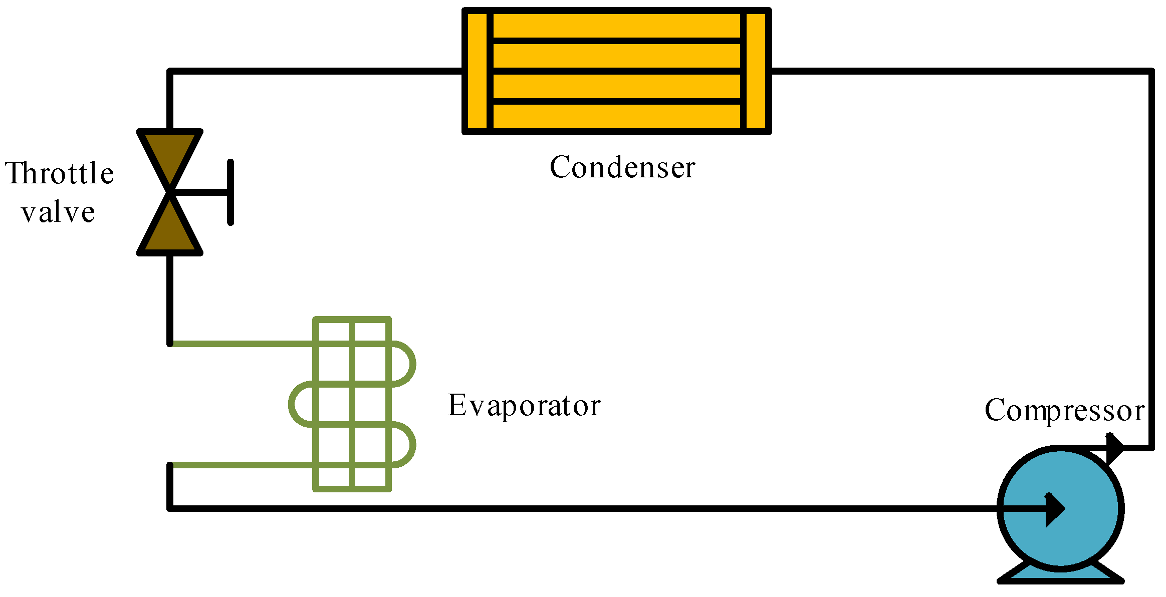
A chiller is a device used to provide cooling and is widely used in air conditioning systems, industrial refrigeration and data center cooling. Its main function is to remove heat through a refrigeration cycle and release it to the external environment through the cooling water system. The chiller typically includes key components such as a compressor, condenser, evaporator and expansion valve. The operation mechanism of the chiller based on the vapor compression refrigeration cycle is shown in Figure 1, which consists of four main steps: Initially, the compressor changes the refrigerant into a vapor with high pressure and high temperature. Next, in the condenser, the refrigerant undergoes condensation into a high-pressure liquid through heat exchange with cooling water. The expansion valve then facilitates the transition of the high-pressure liquid refrigerant into a low-pressure, low-temperature mixture of liquid and gas. Finally, the low-pressure, low-temperature refrigerant absorbs heat from the cooling water or air in the evaporator, thereby completing the cooling process. This is how chillers use refrigerant to cool their surroundings.

Figure 1.
The flow of refrigerant through the chiller [31].
2.2. The Introduction of Chiller’s Faults
There are a variety of faults that may be encountered during chiller operation. Understanding these typical fault patterns can aid in timely maintenance and repair, thereby preventing greater equipment damage and operational interruptions.
Chiller’s fault patterns are shown in Table 1. Poor water quality leads to scale buildup and reduced condenser exchange efficiency produces condenser fouling (CF). Non-condensable gases in the refrigerant (NC) result in the degradation of the refrigerant quality. Various factors can cause different faults. For example, the quantity of refrigerant surpassing the standard value can lead to refrigerant overcharge (RO), while an excess of lubricant can result in excess oil (EO). A refrigerant charge below the standard value will lead to a refrigerant leak (RL). Another example is that improper pump selection, abnormal valve adjustment, or clogged pipes can result in reduced condenser water flow (FWC). This can also lead to reduced evaporator water flow (FEW).

Table 1.
The seven fault patterns and their four fault severity levels.
To summarize, the chiller will produce a variety of faults in actual operation and long-term operation in a faulty state will lead to abnormal system operation, resulting in overload or inefficient operation. As a result, the fault may go undetected for an extended period, leading to increased maintenance costs and production downtime. Moreover, it is not difficult to see from the above arguments that chiller fault problems are related to each other. Xia et al. [19] emphasized the gradual increase in the severity of faults during operation, which suggests that the fault variables have correlation characteristics over time. Therefore, timely and accurate diagnosis of faults is critical.
2.3. Non-Stationary of Chiller Data
Chiller fault diagnosis is a common classification issue. Current studies generally utilize data-driven solutions to tackle this issue. Most of the chiller data are non-stationary, which can reduce the accuracy of classification results. The main reasons for non-stationary chiller data include the following.
- Changes in operating conditions. The chiller operates under different load conditions, resulting in changes in system parameters such as temperature, pressure and flow rate over time, showing non-stationary;
- Influence of external environment. Factors such as variations in external temperature and humidity impact the chiller’s operating status, further exacerbating the non-stationary nature of the data;
- Progressive development of faults. Faults may have a small effect in the initial stage, but the severity of the faults gradually increases over time, leading to non-stationary characteristics of the parameter variations.
In conclusion, a chiller in actual normal operation will have a variety of situation changes, which leads to non-stationary data. Therefore, in the context of fault diagnosis, it is crucial to extract key fault features from dynamic, time-varying, non-stationary data to effectively address the data’s non-stationary characteristics.
2.4. The Basic CA Algorithm
In order to elucidate the long-run equilibrium relationship between the non-stationary variables, this paper used the CA method.
If a non-stationary time series becomes stationary after being differenced d times, it is referred to as being integrated of order d, denoted as . Engel and Granger [32] showed that if a group of non-stationary time series maintains a long-run equilibrium relationship, it can be represented as , where N is the count of non-stationary time series, and U is the count of samples. The data from one sample point are taken and recorded as there exists a vector ; these non-stationary series can be described as
where is the sequence of residuals.
The purpose of CA is to solve for the cointegrating vector . A vector autoregressive (VAR) model was used by Zhao et al. [33] to find the cointegration vector and apply it to a collection of non-stationary variables, given the chiller dataset where N is the count of chiller non-stationary time series, and M is the count of chiller samples. Data from a single sample point are collected and noted as .
The VAR model of can be described as
where is the matrix of coefficients, is the vector of white noise distributed as , is a constant, and p is the order of the VAR model.
The vector error correction (VEC) model is derived by subtracting from both sides of Equation (2).
where ,
Two full rank matrices, and , are obtained by decomposing where . This transformation converts Equations (3) and (4).
The residual sequence is derived in accordance with Equation (4):
According to Zhao et al. [18], the eigenvalue equation can be solved to determine the maximum likelihood estimates of .
where
The coefficients and can be estimated by OLS. The N features are obtained from Equation (6) denoted as . The cointegration vector of the chiller is encapsulated within . The Johansen test yields R cointegrating vectors, from which the cointegration vector matrix can be derived. contains information on the characteristics between the variables and the idea of computing residuals will also be used for subsequent sparse processes.
3. The Suggested Sparse Cointegration Analysis (SCA)
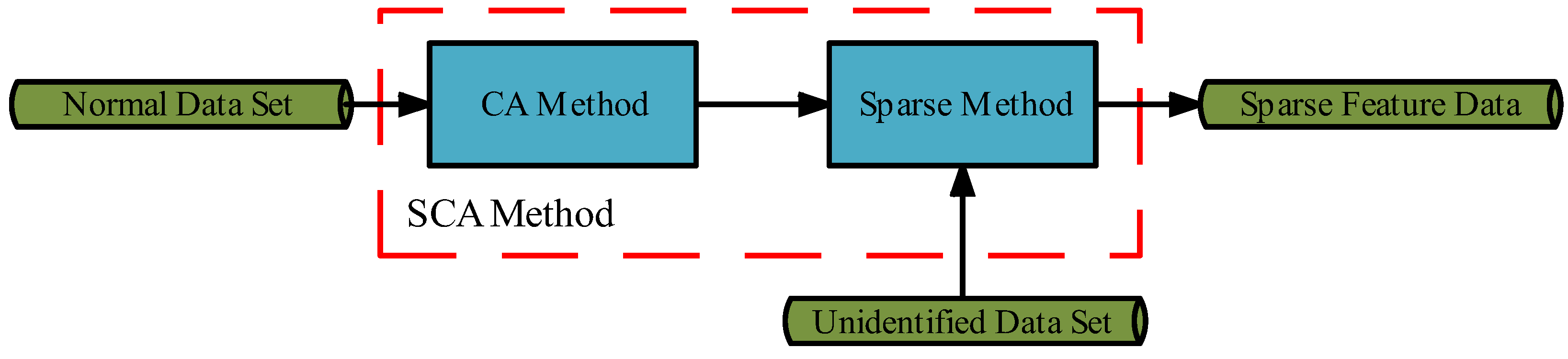
In fault data, not all variables contribute to the fault. Although feature extraction is possible using the CA method, it is not possible to obtain the determining sparse features. Therefore, based on the extracted features in Section 2.4, this paper proposes the SCA method to sparse the feature. As in Figure 2, the SCA method first constructs a cointegration model using the non-stationary dataset obtained by the Augmented Dickey-Fuller (ADF) test [34] strategy. Secondly SCA uses the LASSO method for isolation of the variables in the fault samples to obtain sparse features. The SCA method is described in detail below:
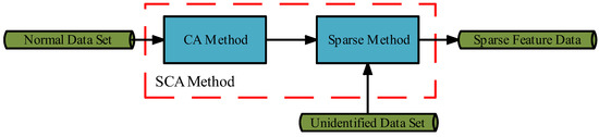
Figure 2.
The process of the SCA method.
A new vector of fault samples to be recognized, , can be factored as follows.
where is the fault-free component, is the standard orthogonal matrix containing the direction of the fault, contains information about the fault magnitude, denotes the fault magnitude, so is the fault component.
Given that not all variables are related to the fault, the process of selecting fault variables can be formulated as the following optimization problem:
where , denote L1 paradigms and is a constant, , where is the chiller data mentioned in Section 2.4. In Equation (8), represents the fault-free component, is denoted as residuals after the removal of fault variables.
Equation (8)’s optimization can be framed as a LASSO regression problem, which relies on the principles of the regression model.
Perform the Cholesky decomposition on
where is the lower triangular matrix.
Then, Equation (8) becomes:
Let , , then Equation (11) solves the LASSO regression problem. This constitutes the problem of variable selection grounded in sparse cointegration.
As stated in Equation (11), the regression coefficient is contingent upon the value of . As increases, more variables are identified as problematic, resulting in more non-zero elements in . Conversely, if is significantly low, many of the coefficients in may be set to zero.
Therefore, in this paper, the coordinate descent method is used to solve the LASSO regression problem, and the regression coefficients can be accurately estimated by addressing the following optimization problem:
where is the loss function of the LASSO regression, k is the number of iterations and Equation (12) is the case of solving for the minimum.
Transform Equations (12) and (13)
According to Equation (13), in order to obtain the optimal , we need to find , which is . Let . Let the canonical representation of column be as follows:
and then obtain
Let , then update the regression coefficients to
Finally, Equation (11) was calculated again based on the resulting . The model was repeatedly fitted for 100 different values of λ, and a 10-fold cross-validation was performed using the cross-validation function to choose the optimal penalty parameter λ. The output of the final algorithm is , i.e., sparse features.
Our main sparse fault variable steps are as follows:
- (1)
- No variables were filtered, and a LASSO regression model was constructed for each fault sample point;
- (2)
- A 10-fold cross-validation is performed using the cross-validation function to select the optimal penalty parameter λ;
- (3)
- Calculate using the optimal λ, i.e., sparse the main features from the LASSO method. Here, since it is solving the smallest solution of Equation (11) it means that it can obtain all the sparse fault features, which is very effective in solving the problem of message propagation between fault variables.
4. An Improved Graph Deviation Network (IGDN) Is Proposed
To address the issue of high correlation among different fault variables in the chiller and to further augment the model’s fault diagnosis capability, this paper adopts the SCA method to extract the features and then further proposes IGDN to classify the fault datasets. The traditional GDN assumes that all data are equally important after graph propagation, which invariably increases the difficulty of the modeling task. To address this issue, the GDN is improved by incorporating CBAM to increase attention on the data, and IGDN is finally proposed.
4.1. Graph Deviation Network (GDN)
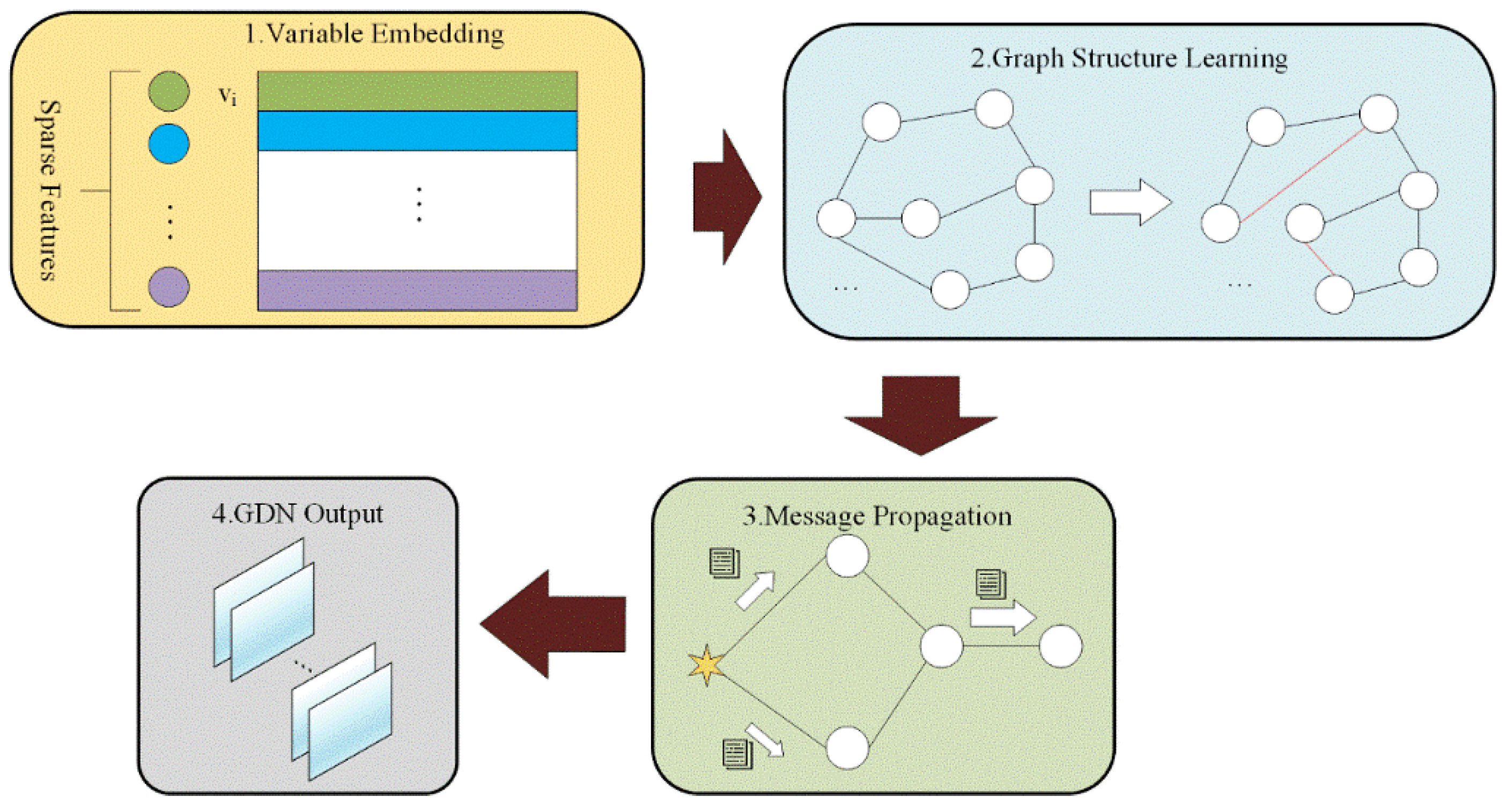
Over time, there is some correlation of features based on SCA after isolating. GDN flexibly captures the unique features of each variable and performs initial processing on the data. In order to flexibly represent the correlation between each different feature, an embedding vector is introduced for each variable to represent its features according to Figure 3:
where is the learnable embedding vector parameter, N is the number of variables, d is the embedding vector dimension, and the ith row of the matrix represents the embedding vector of variable i, i.e., .

Figure 3.
Overview of the GDN framework.
These embedding vectors are initially set randomly and then trained alongside the rest of the model.
To represent the relationship between fault variables, in the absence of a priori information, the candidate relationship for variable i is the set of all variables other than itself :
We compute the similarity between node i’s embedding vector and the embeddings of its candidates .
According to Equation (19), the graph structure of the obtained sparse features is constructed as.
where denotes a directed edge that exists from variable i to variable j, TopK is the index of the top K values in similarity , and K can depend on the number of sparse features.
Aji = 𝟙{j∈TopK ({eki:k∈Ci})}
That is, the GDN first computes the normalized dot product between the embedding vectors of each sparse variable and the candidate relations and index of the K normalized dot product are selected from the top. Based on this index, a graph structure is built up, which will be used for model post-processing.
For the sparse features obtained from SCA, i.e., the features in , retain their original data and set the data of the remaining features to zero. These are combined and denoted .
At moment t, a sliding window of size w is defined to process and the model input are obtained.
The output of the model is the data after processing each moment, denoted as .
In order to capture the relationship between the variables, message propagation is performed based on the information about the graph structure features of the learned nodes and the propagation representation is formulated as follows:
where is denoted as the set of node neighbors obtained from the learned graph. is the trainable weight matrix that is applied to the shared linear transformation at each variable. The coefficients are calculated as follows:
where denotes the concatenation, thus concatenates the vector and the corresponding transformed feature . is a vector of coefficients.
The coefficients are computed using , which functions as a non-linear activation mechanism. This weight-initialized activation function mitigates the problem of vanishing gradients. Compared to the function, solves the neuron death problem of while inheriting the advantages of the function. After calculating the coefficients , the GDN uses the function to normalize the coefficients.
is element-wise multiplied with the corresponding embedding vector to obtain :
where denotes element-wise multiply.
The above is dimensionally transformed and denoted as , which is used as input to the subsequent CBAM for further feature attention.
4.2. Convolutional Block Attention Mechanism (CBAM)
To augment the chiller fault diagnosis model’s ability to dynamically focus on fault data and improve its analysis accuracy, the CBAM is incorporated into the GDN model, forming a fault data attention mechanism.
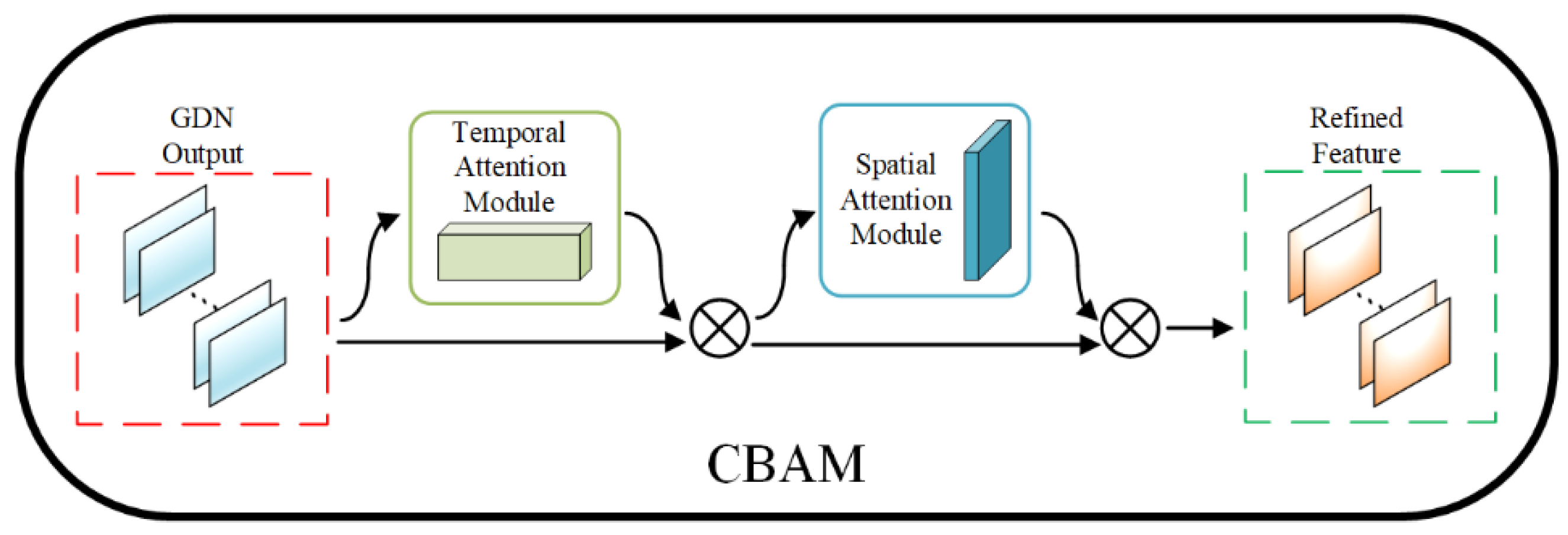
CBAM has the ability to reduce redundant information in feature optimization by paying attention to the data twice to capture extremely subtle correlations within the data. Figure 4 shows the overall process of CBAM.
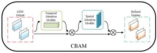
Figure 4.
The overview of CBAM [27].
As shown in Figure 4, the output of the given GDN, i.e., the intermediate feature data , is used as the input to CBAM. Where C denotes the number of variables, and H × W represents GDN preliminary processed data.
Temporal attention significantly enhances the network’s representation by integrating both average and maximum pooling features. These operations, referred to as and , are denoted as the average pooled features and maximum pooled features, respectively. These two descriptors are then processed through a multi-layer perceptron (MLP) with shared weights to generate two feature maps. The hidden layer activation size is set to , and r is the decay ratio. Finally, the temporal attention map is computed by element-by-element summation with a sigmoid function. The temporal attention is computed as:
where denotes the sigmoid function, ,.
The output of the temporal attention module is , which serves as the input to the spatial attention module.
Spatial attention was performed after temporal attention. It generates two two-dimensional feature maps by performing averaging and maximum pooling operations on the temporal dimension of the input feature maps of the chiller: and . These two feature maps are then processed through a convolutional layer to obtain the final spatial attention map using a sigmoid function.
where denotes the sigmoid function, denotes a convolution operation with a filter size of 7 × 7.
The final CBAM output is .
Given the GDN processed data, CBAM computes complementary attention through two attention modules, temporal and spatial, focusing on “what” and “where”, respectively. Eventually, the two modules are sequentially sorted, and temporal attention is prioritized for computation. Finally, the results of CBAM processing all variable data are fed into the fully connected layers to successfully achieve high-accuracy classification.
5. Proposed SCA-IGDN Based on Chiller Fault Diagnosis Method
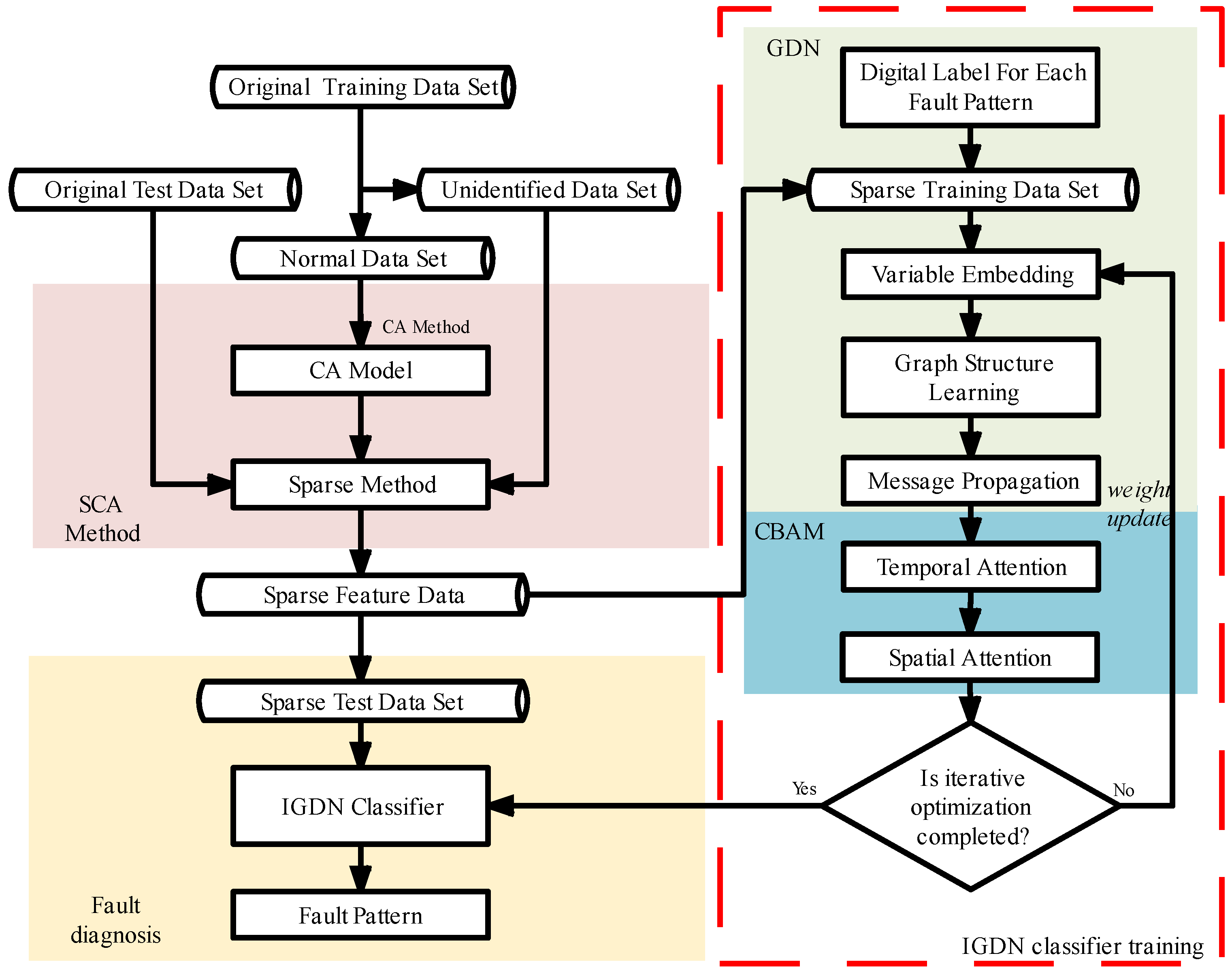
This section synthesizes the content of Section 3 and Section 4 and proposes the SCA-IGDN method. The flowchart of the chiller fault diagnosis strategy, utilizing the SCA-IGDN method, is presented in Figure 5, which includes five main steps: the SCA obtaining sparse features, the GDN building graph structure, the CBAM increasing focus on data, the IGDN classifier training model and fault diagnosis. Specifically, the steps to achieve this are as follows:

Figure 5.
The strategy flow of the SCA-IGDN-based chiller fault diagnosis method.
- (1)
- SCA obtains sparse features. In the original training dataset, the chiller data mostly reflect non-stationary characteristics, and most of the existing methods assume the chiller data to be stationary, which cannot accurately identify the normal operation changes from the real dynamic anomalies. For this reason, the SCA method is proposed to extract and obtain the features in non-stationary processes. The sparse feature data is used as a new training dataset;
- (2)
- GDN builds graph structures. The sparse feature data based on SCA isolating are fed to the classifier and vectors are embedded for each sparse variable to flexibly capture its unique features. Further, graph structures are created for learning to represent correlations between variables. Finally, the message propagation of the graph gives the deviation of each variable from its neighbors;
- (3)
- CBAM increases the attention to data. The dimensional transformation of the output data from the GDN is followed by the application of CBAM. This process applies attention to both the temporal and spatial dimensions of the feature data, identifying the key features that influence various faults. Finally, the output of the CBAM is fed into the fully connected layers for training;
- (4)
- Complete the training of the IGDN classifier. These include sparse training datasets after isolating, and the corresponding labels are fed into the IGDN classifier for training. The application of training data is optimized by constantly updating the weights of each parameter, which leads to accurate recognition of different data until the training is halted upon reaching a specified number of iterations;
- (5)
- Fault diagnosis is realized by the IGDN classifier. Sparse fault data are utilized as a sparse test dataset. The sparse test dataset is fed into the trained IGDN classifier to diagnose chiller fault patterns.
6. Experiment and Comparison
6.1. Description of the Chiller Dataset
The dataset in this paper, derived from the ASHRAE 1043 project [31], originates from an experiment on a 90 ton chiller operating with R134a refrigerant, collecting data on 64 process variables at 10 s intervals.
The fault diagnosis capability of the proposed SCA-IGDN method is thoroughly validated in this paper utilizing 16 chiller process variables, which are listed in Table 2 based on the research of the ASHRAE 1043 project.
Table 2.
The description of the selected process variables.
Seven distinct fault patterns are included in the dataset, each represented by different abbreviations, as detailed in Table 1. In order to simulate the non-stationary nature of the data and to describe the long-term equilibrium relationship between the different variables, each fault datum was randomly and continuously sampled. To thoroughly evaluate the performance of the proposed SCA-IGDN method, the original dataset is divided into four distinct subsets: Level 1, Level 2, Level 3 and Level 4, each representing different severity levels. The four subsets range in severity from minor to severe, with each subset including seven typical fault data and a set of normal operation data. Table 1 provides the details of the seven typical fault patterns across different severity levels, along with their abbreviations.
The CA model is built by applying 1000 data under normal operation, the normal dataset in Figure 5. Six hundred data under normal operation and 600 data for each fault pattern under each level are selected for the training of each experimental classifier. Two hundred data under normal operation and 200 data for each fault pattern under each level are selected to serve as the test dataset for every model. Finally, four sets of datasets (corresponding to the four levels) are built up for detailed experiments. The symbol “Normal” denotes the data representing normal operation.
6.2. Fault Diagnosis Performance Evaluation Index
Two classical evaluation metrics are employed to effectively evaluate and compare the effectiveness of the diagnostic models. Recall (R) and precision (P) are used to independently assess the different models. These metrics are detailed in Table 3.
Table 3.
Evaluation index confusion matrix.
Performance metrics R and P are used for binary classification. Each fault pattern is treated as a positive example, with others considered negative. These metrics can be directly applied to data corresponding to any fault pattern. To assess the overall effectiveness of the model across each severity level, the recall and accuracy at each level are averaged to obtain the average recall and the average accuracy .
6.3. Parameters Setting
For fault variable extraction, CA is calculated to obtain B(16 × 4). The LASSO regression penalty parameters in this paper are selected by the coordinate descent method adaptive optimization.
Regarding the parameter settings of IGDN, the sliding window value was set to 5 steps of 1. The TopK was chosen to be from 2 to 4 (selected according to the different severity levels) as the sparse variables have been acquired. Dropout is set to be 0.2, and 64-dimensional embedding vectors are applied. The convolution kernel of CBAM is set to be 7, and 80 hidden neurons are used in the output layer. 20% of the IGDN training dataset is taken out as a validation dataset, and Adam [35] optimizer is applied to optimize the parameters.
6.4. The Analysis of Information Propagation between Fault Variables in CF at Different Fault Severity Levels
Propagation of faults across variables leads to increased correlation between them. In this Section, Level 1 and Level 4 datasets will be used to demonstrate the phenomenon of correlation between fault variables in chiller. Further evidence of the feasibility of applying the graph structure.
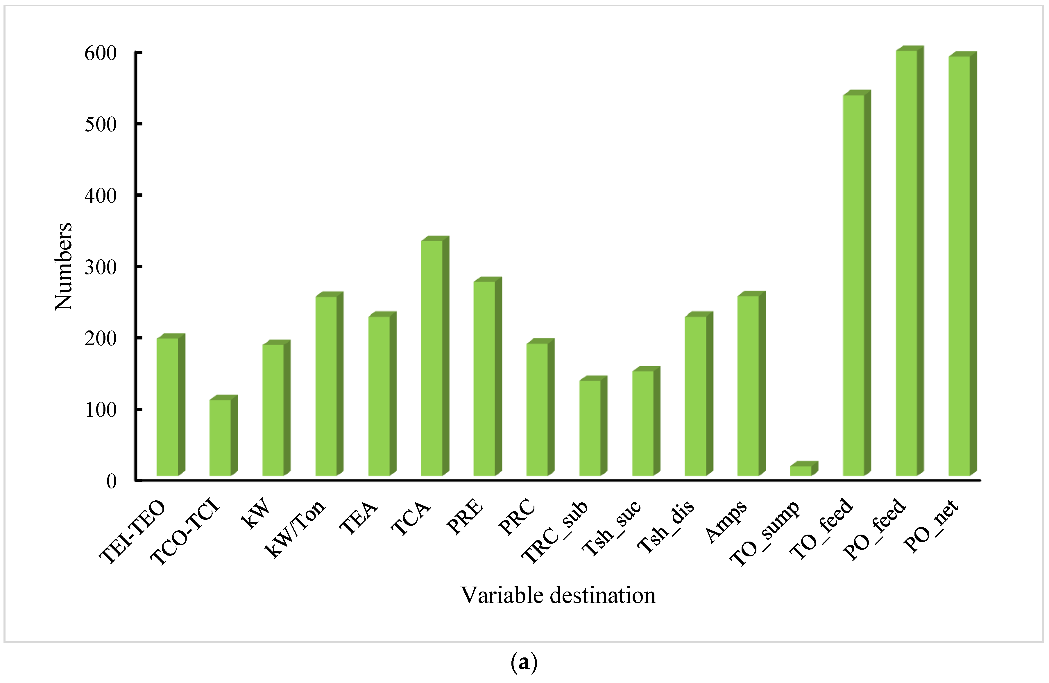
Figure 6a,b shows the bar charts of the frequency of each fault variable being selected in Level 1 and Level 4 obtained using the SCA method, respectively. The variable names are represented on the horizontal axis, and the vertical axis shows the frequency of each variable’s selection. It can be seen that the three main fault variables, TO_feed, PO_feed and PO_net, represent the occurrence of CF in Level 1 and Level 4. In Figure 6b, there is a significant increase in the number of filters for the TCA variable compared to (a) due to the elevation of fault severity level. Meanwhile, there is a small increase in the number of variables TEI-TEO, TCO-TCI and TEA filtered in relation to the temperature parameters, which represents the propagation of faults across variables. Further evidence of the feasibility of the IGDN classifier is proposed after the SCA process.
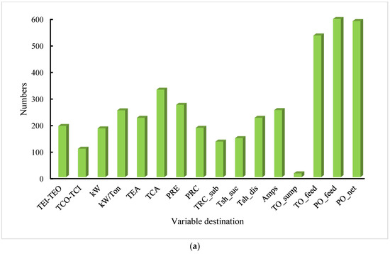
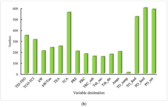
Figure 6.
Selection frequency for each variable at Level 1 and Level 4 was obtained using the SCA method. (a) Selection frequency for each variable at Level 1. (b) Selection frequency for each variable at Level 4.
6.5. Comparison of the Performance of Different Models
6.5.1. Performance Comparison of Fault Variable Extraction
The proposed SCA method’s superior performance in extracting fault variables is thoroughly demonstrated through a comparison with principal component analysis (PCA). The unprocessed original data are initially fed into the IGDN and recorded as the first model. Similarly, the PCA based on the IGDN model, denoted as PCA-IGDN, is constructed by combining the established PCA method with the IGDN classifier. Finally, the adopted SCA method is combined with the IGDN classifier proposed in this paper, denoted as SCA-IGDN. Level 2 dataset is selected to evaluate the effectiveness of IGDN, PCA-IGDN and SCA-IGDN. In this way, the SCA method can be analyzed in fault diagnosis ability.
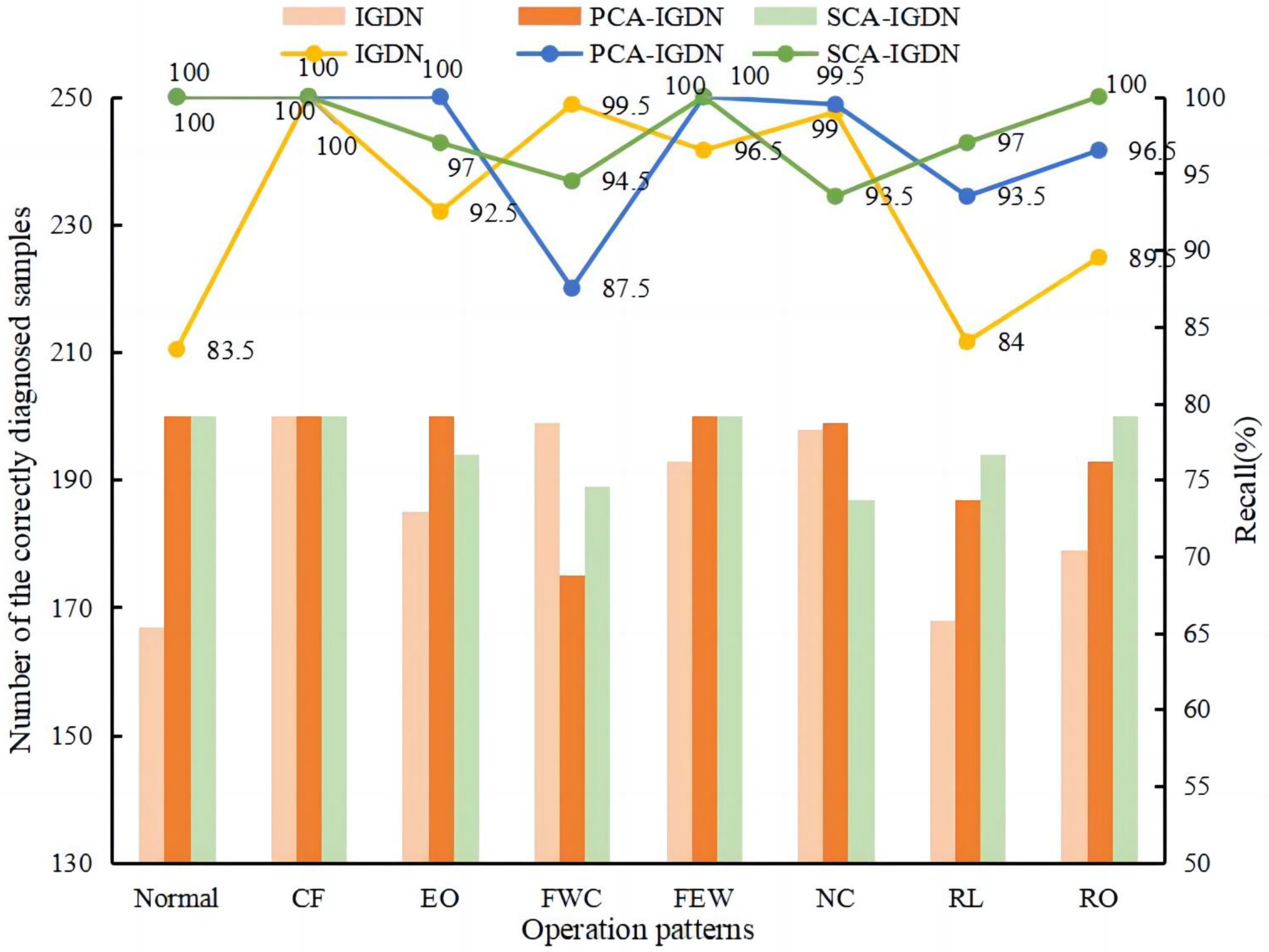
Figure 7 illustrates the diagnostic outcomes of the three models for the different operation patterns. The chiller operation patterns are depicted on the horizontal axis. The left vertical axis displays the number of correctly classified samples, whereas the right vertical axis represents the recall for chiller fault diagnosis. From the figure, it is evident that the proposed SCA-IGDN model performs well in terms of recall compared to both the IGDN and PCA-IGDN models when diagnosing faults across all eight operation patterns of the chiller. Compared to the results shown in Figure 7 and analyzed in Table 4, the SCA-IGDN model has the highest recall for Normal, CF, FEW, RL and RO operation patterns. Moreover, the most notable enhancement in recall was observed in the three operation patterns: Normal, RL, and RO. Meanwhile, in the RL classification, the recall of the SCA-IGDN model is enhanced by 3.5% compared to the IGDN model and by 9.5% over the PCA-IGDN model.
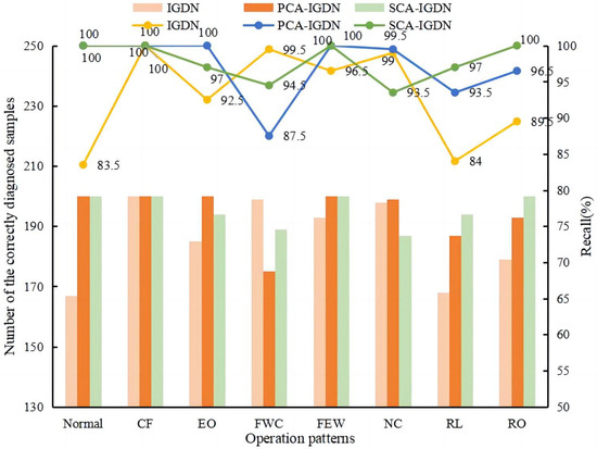
Figure 7.
Comparison results of the IGDN, PCA-IGDN and SCA-IGDN models using the Level 2 dataset.
Table 4.
Performance comparison of the IGDN, PCA-IGDN and SCA-IGDN models utilizing the Level 2 dataset.
In summary, compared with the PCA, the SCA method in fault diagnosis has a very bright performance in the extraction of fault variables, and it has a better fault diagnosis performance. This is because the SCA method notices fault variables in non-stationary processes and extracts them.
6.5.2. Performance Comparison of Classifier Capabilities
To assess the fault diagnosis performance of IGDN, a comparison is made with GDN and long short-term memory (LSTM) classifiers. For a fair comparison, the sparse features obtained after SCA are fed to the GDN, LSTM and IGDN classifiers, respectively. The three classifiers are denoted as SCA-GDN, SCA-LSTM and SCA-IGDN. In the experiments, the validity of SCA-GDN, SCA-LSTM and SCA-IGDN continued to be evaluated by using the Level 2 dataset.
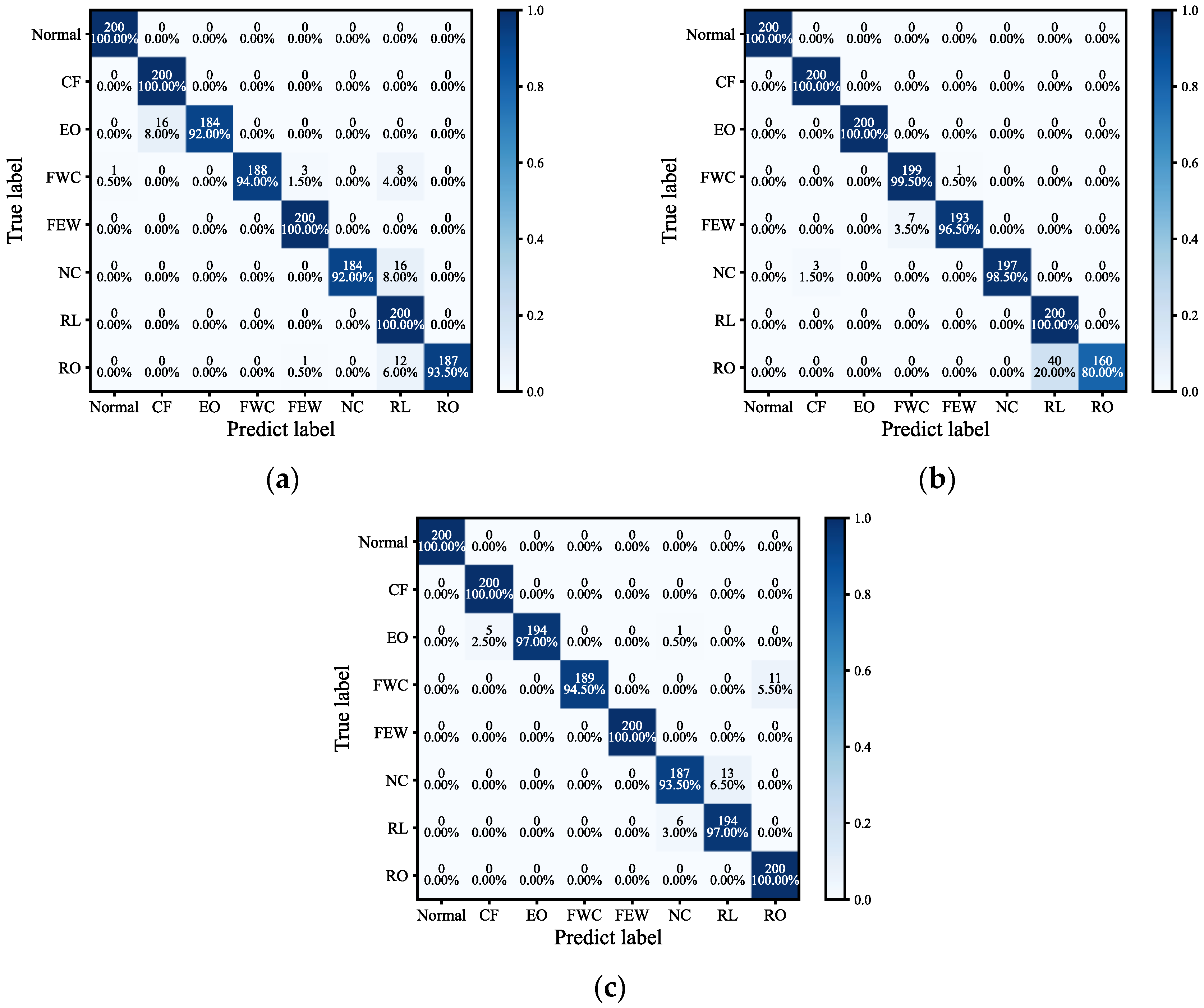
Figure 8 presents the confusion matrix of the outcomes of the fault diagnosis for the three classifiers. According to Figure 8, the blue squares represent the number of samples allocated for fault diagnosis. The percentile represents the percentage of diagnostic classifications in the eight actual operation patterns. Comparing Figure 8a,c, the fault diagnosis R-value of the SCA-IGDN model is better than the SCA-GDN model. In addition, according to Figure 8b, the SCA-LSTM model has a low R-value for RO, while the SCAI-GDN model significantly improves the R-value for fault diagnosis.
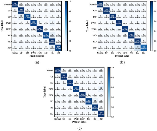
Figure 8.
Diagnosis results of the GDN, SCA-LSTM and SCA-IGDN models using the Level 2 dataset. (a) SCA-GDN; (b) SCA-LSTM; (c) SCA-IGDN.
Table 5 calculates the R-value and p-value of SCA-GDN, SCA-LSTM and SCA-IGDN. The R-value and p-value of the three models at Level 2 are derived from the confusion matrix of Figure 8. According to Table 5, the R-value and p-value of the SCA-IGDN model are higher than those of the SCA-GDN model and the SCA-LSTM model at Level 2. In addition, the SCA-IGDN model has a more significant improvement in the p-value among the fault diagnosis of RL, which is 8.97% and 10.39% higher compared to the SCA-GDN and SCA-LSTM models, respectively. Furthermore, the comparison between IGDN and LSTM shows that IGDN has superior performance in dealing with the correlation problem between variables. In summary, the IGDN classifier yields the optimal R-value and p-value when the SCA method is used, which demonstrates that the IGDN classifier proposed in this paper exhibits excellent fault diagnosis performance.
Table 5.
Performance comparison of the SCA-GDN, SCA-LSTM and SCA-IGDN models utilizing the Level 2 dataset.
6.6. Analysis of Model Diagnostic Capabilities for Different Fault Severity Levels
In order to verify that the proposed SCA-IGDN model exhibits superior performance under different fault severity levels, this section analyzes and compares GDN, LSTM, PCA-GDN and SCA-IGDN in detail.
6.6.1. Comparison of Severity Level 1
Faults at Level 1 occur earlier compared to other fault severity levels, resulting in less obvious faults. Therefore, a larger gap in fault diagnostic performance between the different models, which will be reflected in the p-value and R-value for the different operation patterns. Overall, the SCA-IGDN demonstrates an excellent ability to recognize subtle fault variables in the early stages.
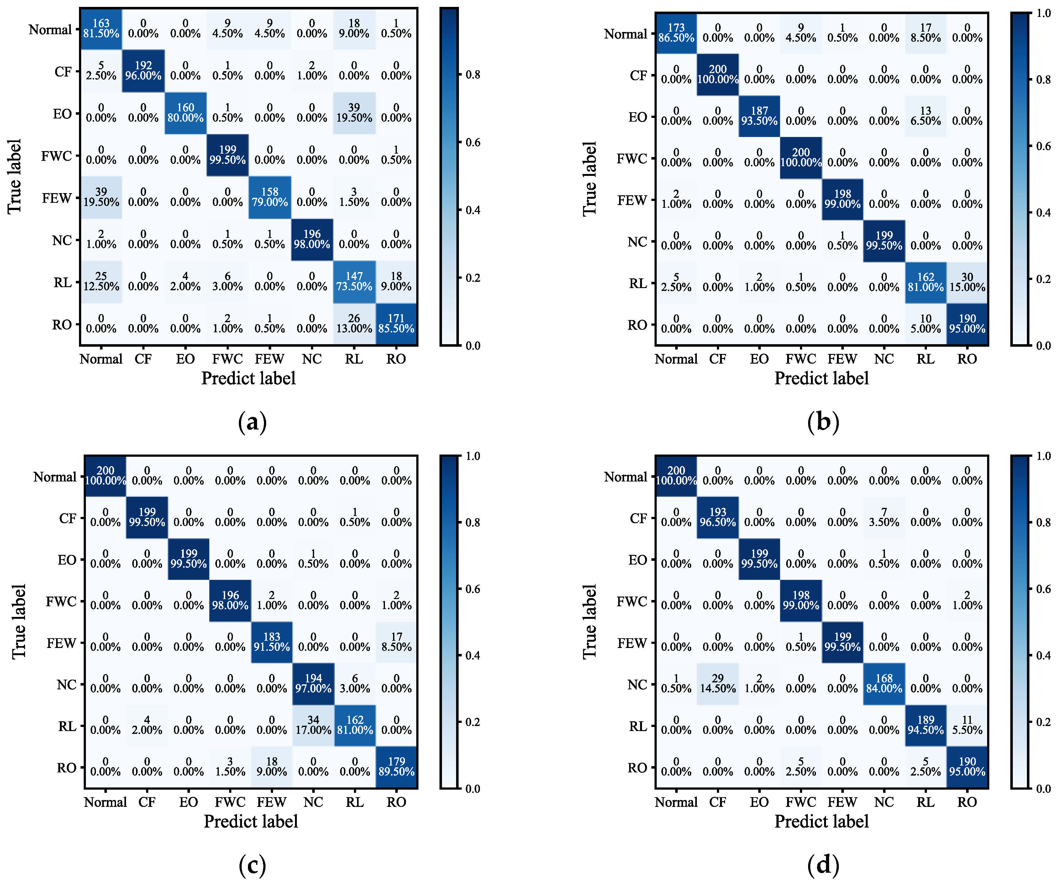
The confusion matrix displaying the fault diagnosis outcomes at Level 1 for the four models is presented in Figure 9. The figure reveals that the GDN, LSTM, and PCA-GDN models exhibit lower accuracy in the last two rows of Figure 9a–c. This misclassification suggests that a significant portion of RO and RL samples are erroneously identified as other fault patterns by these models. Moreover, Figure 9a,b displays a significantly higher count of misdetections compared to Figure 9c,d, indicating a greater tendency for fault samples to be erroneously categorized as different fault patterns. Among the four models, the SCA-IGDN model exhibits the highest classification accuracy.
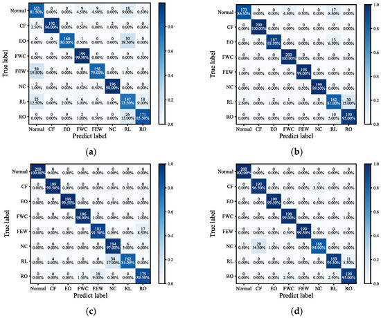
Figure 9.
Diagnosis results of the GDN, LSTM, PCA-GDN and SCA-IGDN models using the Level 1 dataset. (a) GDN; (b) LSTM; (c) PCA-GDN; (d) SCA-IGDN.
For further comparison, Table 6 lists the p-value and R-value of GDN, LSTM, PCA-GDN and SCA-IGDN based on Figure 9 calculation. Table 6 demonstrates that the SCA-IGDN model achieves the highest average p-value and R-value across different operation pattern datasets. Consequently, the experiments depicted in Figure 9 and the data provided in Table 6 substantiate that the proposed SCA-IGDN model demonstrates superior fault diagnosis performance compared to the GDN, LSTM, and PCA-GDN models.
Table 6.
The R-value and p-value across various fault patterns are depicted for all four models.
6.6.2. Overall Comparison of the Four Levels
In order to further compare the superiority of the SCA-IGDN model, this section compares the fault diagnosis results of the four fault severity levels in general and calculates the average R-value and p-value of the GDN, LSTM, PCA-GDN and SCA-IGDN for each of the four fault levels. Table 7 represents the average R-value and p-value of fault diagnosis for GDN, LSTM, PCA-GDN and SCA-IGDN under four fault severity levels, as well as the obtained and . It can be seen from Table 7 that the and of SCA-IGDN are higher than those of GDN, LSTM and PCA-GDN, i.e., the SCA-IGDN model shows its superiority in general.
Table 7.
Average R-value and p-value for the four models evaluated at various fault severity levels.
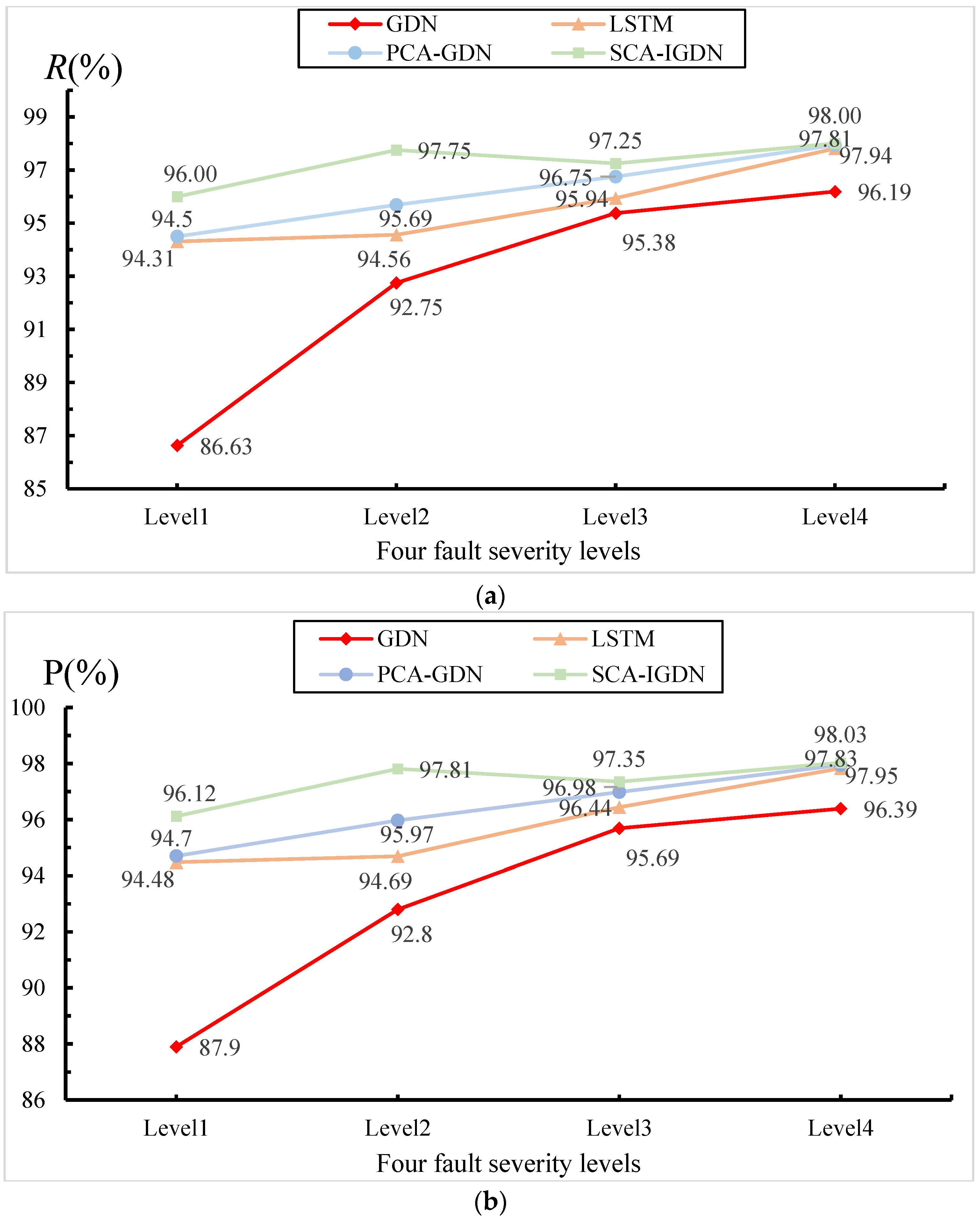
The average R-value and p-value of fault diagnosis under four fault severity levels for each model are plotted below according to Table 7. Figure 10a,b, the horizontal axis represents the four fault severity levels, and the vertical axis represents the R-value and p-value for each fault severity level, respectively. Figure 10 illustrates that the SCA-IGDN model exhibits superior R-value and p-value metrics across all four fault severity levels. In addition, among the four models for diagnosis, the SCA-IGDN model showed the most significant improvement in diagnostic performance for Level 1. In terms of R-value, the SCA-IGDN model improved by 9.37% compared to the GDN model, 1.69% compared to the LSTM model and 1.50% compared to the PCA-GDN model. In terms of p-value, the SCA-IGDN model improved by 8.22% compared to the GDN model, 1.64% compared to the LSTM model and 1.42% compared to the PCA-GDN model. This indicates that the SCA-IGDN model can accurately diagnose the faults at the early stages of their occurrence.
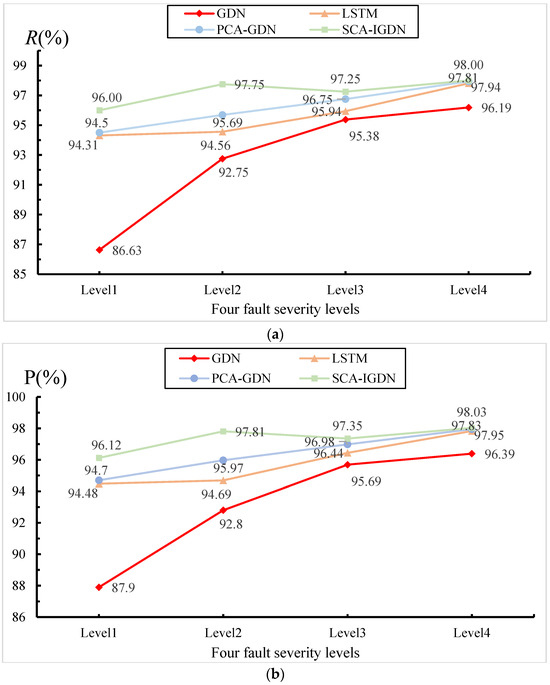
Figure 10.
The average for the R-value and p-value of the four models for different fault severity levels. (a) The average for the R-value of the four models for different fault severity levels; (b) The average for the p-value of the four models for different fault severity levels.
7. Conclusions
This study presents the SCA-IGDN method, a novel approach designed to enhance chiller fault diagnosis performance in non-stationary data environments. The SCA-IGDN method employs the developed SCA method, while the IGDN model is proposed in order to augment the diagnosis accuracy. SCA-IGDN demonstrates the capability to accurately extract sparse non-stationary features and derive fault decision features without relying on historical fault data. The feasibility and efficacy of SCA-IGDN are established through comprehensive comparative analyses against multiple models.
The primary contributions of this research are three-fold. Firstly, we capture the long-run equilibrium relationships between non-stationary variables and obtain sparse features. Secondly, a graph structure is created for the sparse correlation features. Finally, to increase the diagnosis accuracy, CBAM is incorporated into the GDN classifier to increase the attention to the data. On the ASHRAE 1043 dataset, by overall comparison with GDN, LSTM, and PCA-GDN methods, it is verified that the proposed SCA-IGDN method embodies excellent performance in chiller fault diagnosis based on non-stationary data. Specifically, the comparison with IGDN and PCA-IGDN demonstrates that the SCA method of the proposed SCA-IGDN model exhibits superior results in dealing with non-stationary data. In addition, compared with SCA-GDN and SCA-LSTM, it is demonstrated that the IGDN model exhibits superior performance in dealing with correlation features as well as enhancing data attention. To further demonstrate the feasibility of the proposed classifier after the SCA process, the paper concludes with detailed experiments on the propagation of faults across variable problems. The results reveal significant improvements in diagnostic R-value and p-value using the SCA-IGDN-based fault diagnosis method, thereby substantiating its accuracy.
It is noteworthy that the applicability of the proposed SCA-IGDN method extends beyond chiller fault diagnosis to other non-stationary operating systems, highlighting its versatility and potential for broader implementation. However, future research should focus on further reducing the computational complexity of the SCA-IGDN method to facilitate its practical application in real-world scenarios.
In addition, in the actual operation of the chiller, multiple faults may occur at the same time. Conventional fault diagnosis cannot recognize multiple faults. In future research, for this problem, advanced deep learning models can be utilized to capture the correlation features among different faults from complex high latitude data to achieve multiple fault diagnosis.
Author Contributions
Conceptualization, B.S.; Investigation, B.S., D.L. and H.Z.; Software, B.S. and D.L.; Methodology, D.L. and H.Z.; Project administration, H.Z.; Supervision, H.Z.; Funding acquisition, H.Z. All authors have read and agreed to the published version of the manuscript.
Funding
This research is partially funded by the Youth Innovation Technology Project of Higher School in Shandong Province (No. 2022KJ204), the National Natural Science Foundation of China (62003191) and the Natural Science Foundation of Shandong Province (ZR2020QF072). The APC was funded by (No. 2022KJ204).
Data Availability Statement
Our data is unavailable due to privacy or ethical restrictions.
Conflicts of Interest
The authors declare no conflict of interest.
References
- Shen, C.; Zhang, H.; Meng, S.; Li, C. Augmented data driven self-attention deep learning method for imbalanced fault diagnosis of the HVAC chiller. Eng. Appl. Artif. Intell. 2023, 117, 105540. [Google Scholar] [CrossRef]
- Li, G.; Xiong, J.; Tang, R.; Sun, S.; Wang, C. In-situ sensor calibration for building HVAC systems with limited information using general regression improved Bayesian inference. Build. Environ. 2023, 234, 110161. [Google Scholar] [CrossRef]
- Chen, T.; An, Y.; Heng, C.K. A review of building-integrated photovoltaics in Singapore: Status, barriers, and prospects. Sustainability 2022, 14, 10160. [Google Scholar] [CrossRef]
- Li, G.; Chen, L.; Liu, J.; Fang, X. Comparative study on deep transfer learning strategies for cross-system and cross-operation-condition building energy systems fault diagnosis. Energy 2023, 263, 125943. [Google Scholar] [CrossRef]
- Zhu, X.; Chen, K.; Anduv, B.; Jin, X.; Du, Z. Transfer learning based methodology for migration and application of fault detection and diagnosis between building chillers for improving energy efficiency. Build. Environ. 2021, 200, 107957. [Google Scholar] [CrossRef]
- Schmid, M.; Gebauer, E.; Hanzl, C.; Endisch, C. Active model-based fault diagnosis in reconfigurable battery systems. IEEE Trans. Power Electron. 2020, 36, 2584–2597. [Google Scholar] [CrossRef]
- Hasan, A.; Tahavori, M.; Midtiby, H.S. Model-based fault diagnosis algorithms for robotic systems. IEEE Access 2023, 11, 2250–2258. [Google Scholar] [CrossRef]
- Chen, L.; Li, G.; Liu, J.; Liu, L.; Zhang, C.; Gao, J.; Xu, C.; Fang, X.; Yao, Z. Fault diagnosis for cross-building energy systems based on transfer learning and model interpretation. J. Build. Eng. 2024, 91, 109424. [Google Scholar] [CrossRef]
- Xu, Y.; Ge, X.; Guo, R.; Shen, W. Recent Advances in Model-Based Fault Diagnosis for Lithium-Ion Batteries: A Comprehensive Review. arXiv 2024, arXiv:2401.16682. [Google Scholar]
- Zhou, Z.; Chen, H.; Li, G.; Zhong, H.; Zhang, M.; Wu, J. Data-driven fault diagnosis for residential variable refrigerant flow system on imbalanced data environments. Int. J. Refrig. 2021, 125, 34–43. [Google Scholar] [CrossRef]
- Gao, Y.; Han, H.; Lu, H.; Jiang, S.; Zhang, Y.; Luo, M. Knowledge mining for chiller faults based on explanation of data-driven diagnosis. Appl. Therm. Eng. 2022, 205, 118032. [Google Scholar] [CrossRef]
- Yang, W.; Zhang, H.; Lim, J.B. Fault Diagnosis of the Chiller Under Imbalanced Data Environment via Combining an Improved GAN and the Random Forest Algorithm. In Proceedings of the 2023 China Automation Congress (CAC), Chongqing, China, 17–19 November 2023; pp. 7390–7395. [Google Scholar]
- Shahnazari, H.; Mhaskar, P.; House, J.M.; Salsbury, T.I. Modeling and fault diagnosis design for HVAC systems using recurrent neural networks. Comput. Chem. Eng. 2019, 126, 189–203. [Google Scholar] [CrossRef]
- Li, G.; Wang, L.; Shen, L.; Chen, L.; Cheng, H.; Xu, C.; Li, F. Interpretation of convolutional neural network-based building HVAC fault diagnosis model using improved layer-wise relevance propagation. Energy Build. 2023, 286, 112949. [Google Scholar] [CrossRef]
- Li, T.; Zhao, Y.; Zhang, C.; Luo, J.; Zhang, X. A knowledge-guided and data-driven method for building HVAC systems fault diagnosis. Build. Environ. 2021, 198, 107850. [Google Scholar] [CrossRef]
- Zhang, H.; Yang, W.; Yi, W.; Lim, J.B.; An, Z.; Li, C. Imbalanced data based fault diagnosis of the chiller via integrating a new resampling technique with an improved ensemble extreme learning machine. J. Build. Eng. 2023, 70, 106338. [Google Scholar] [CrossRef]
- e Silva, P.C.L.; Junior, C.A.S.; Alves, M.A.; Silva, R.; Cohen, M.W.; Guimarães, F.G. Forecasting in non-stationary environments with fuzzy time series. Appl. Soft Comput. 2020, 97, 106825. [Google Scholar] [CrossRef]
- Sun, H.; Zhang, S.; Zhao, C.; Gao, F. A sparse reconstruction strategy for online fault diagnosis in nonstationary processes with no a priori fault information. Ind. Eng. Chem. Res. 2017, 56, 6993–7008. [Google Scholar] [CrossRef]
- Xia, Y.; Zhao, J.; Ding, Q.; Jiang, A. Incipient chiller fault diagnosis using an optimized least squares support vector machine with gravitational search algorithm. Front. Energy Res. 2021, 9, 755649. [Google Scholar] [CrossRef]
- Chen, D.; Liu, R.; Hu, Q.; Ding, S.X. Interaction-aware graph neural networks for fault diagnosis of complex industrial processes. IEEE Trans. Neural Netw. Learn. Syst. 2021, 34, 6015–6028. [Google Scholar] [CrossRef]
- Nguyen BL, H.; Vu, T.V.; Nguyen, T.T.; Panwar, M.; Hovsapian, R. Spatial-temporal recurrent graph neural networks for fault diagnostics in power distribution systems. IEEE Access 2023, 11, 46039–46050. [Google Scholar] [CrossRef]
- Fan, C.; Lin, Y.; Piscitelli, M.S.; Chiosa, R.; Wang, H.; Capozzoli, A.; Ma, Y. Leveraging graph convolutional networks for semi-supervised fault diagnosis of HVAC systems in data-scarce contexts. Build. Simul. 2023, 16, 1499–1517. [Google Scholar] [CrossRef]
- Deng, A.; Hooi, B. Graph neural network-based anomaly detection in multivariate time series. In Proceedings of the AAAI Conference on Artificial Intelligence, virtually, 20–27 February 2021; Volume 35, pp. 4027–4035. [Google Scholar]
- Li, Z.; Fan, R.; Tu, J.; Ma, J.; Ai, J.; Dong, Y. TDANet: A Novel Temporal Denoise Convolutional Neural Network with Attention for Fault Diagnosis. arXiv 2024, arXiv:2403.19943. [Google Scholar]
- Li, P. A Multi-scale Attention-Based Transfer Model for Cross-bearing Fault Diagnosis. Int. J. Comput. Intell. Syst. 2024, 17, 42. [Google Scholar] [CrossRef]
- Fahim, S.R.; Sarker, Y.; Sarker, S.K.; Sheikh, R.I.; Das, S.K. Self attention convolutional neural network with time series imaging based feature extraction for transmission line fault detection and classification. Electr. Power Syst. Res. 2020, 187, 106437. [Google Scholar] [CrossRef]
- Woo, S.; Park, J.; Lee, J.Y.; Kweon, I.S. Cbam: Convolutional block attention module. In Proceedings of the European Conference on Computer Vision (ECCV), Munich, Germany, 8–14 September 2018; pp. 3–19. [Google Scholar]
- Zhang, Q.; Wei, X.; Wang, Y.; Hou, C. Convolutional Neural Network with Attention Mechanism and Visual Vibration Signal Analysis for Bearing Fault Diagnosis. Sensors 2024, 24, 1831. [Google Scholar] [CrossRef] [PubMed]
- Wu, J.; Kong, L.; Kang, S.; Zuo, H.; Yang, Y.; Cheng, Z. Aircraft Engine Fault Diagnosis Model Based on 1DCNN-BiLSTM with CBAM. Sensors 2024, 24, 780. [Google Scholar] [CrossRef] [PubMed]
- Qin, H.; Pan, J.; Li, J.; Huang, F. Fault diagnosis method of rolling bearing based on CBAM_ResNet and ACON activation function. Appl. Sci. 2023, 13, 7593. [Google Scholar] [CrossRef]
- Braun, J.E.; Comstock, M.C. Development of Analysis Tools for the Evaluation of Fault Detection and Diagnostics for Chillers. Deliverable for ASHRAE Research Project. 1999. Available online: https://store.accuristech.com/ashrae/standards/rp-1043-fault-detection-and-diagnostic-fdd-requirements-and-evaluation-tools-for-chillers?product_id=1716217 (accessed on 10 August 2024).
- Engle, R.F.; Granger, C.W.J. Co-integration and error correction: Representation, estimation, and testing. Econom. J. Econom. Soc. 1987, 55, 251–276. [Google Scholar] [CrossRef]
- Yu, W.; Zhao, C.; Huang, B. Recursive cointegration analytics for adaptive monitoring of nonstationary industrial processes with both static and dynamic variations. J. Process Control. 2020, 92, 319–332. [Google Scholar] [CrossRef]
- Ajewole, K.P.; Adejuwon, S.O.; Jemilohun, V.G. Test for stationarity on inflation rates in Nigeria using augmented dickey fuller test and Phillips-persons test. J. Math. 2020, 16, 11–14. [Google Scholar]
- Reyad, M.; Sarhan, A.M.; Arafa, M. A modified Adam algorithm for deep neural network optimization. Neural Comput. Appl. 2023, 35, 17095–17112. [Google Scholar] [CrossRef]

Disclaimer/Publisher’s Note: The statements, opinions and data contained in all publications are solely those of the individual author(s) and contributor(s) and not of MDPI and/or the editor(s). MDPI and/or the editor(s) disclaim responsibility for any injury to people or property resulting from any ideas, methods, instructions or products referred to in the content. |
© 2024 by the authors. Licensee MDPI, Basel, Switzerland. This article is an open access article distributed under the terms and conditions of the Creative Commons Attribution (CC BY) license (https://creativecommons.org/licenses/by/4.0/).