Abstract
Biomass supply chain (BSC) activities have caused social and environmental disruptions, such as climate change, energy security issues, high energy demand, and job opportunities, especially in rural areas. Moreover, different economic problems have arisen globally in recent years (e.g., the high costs of BSC logistics and the inefficiency of generating bioenergy from low-energy-density biomass). As a result, numerous researchers in this field have focused on modeling and optimizing sustainable BSC. To this end, this study aims to develop a multi-objective mathematical model by addressing three sustainability pillars (economic cost, environmental emission, and job creation) and three decision levels (i.e., strategic (location of facilities), tactical (type of transportation and routing), and operational (vehicle planning). A palm oil BSC case study was selected in the context of Malaysia in which two advanced evolutionary algorithms, i.e., non-dominated sorting genetic algorithm II (NSGA-II) and Multiple Objective Particle Swarm Optimization (MOPSO), were implemented. The study results showed that the highest amounts of profit obtained from the proposed supply chain (SC) design were equal to $13,500 million and $7000 million for two selected examples with maximum emissions. A better target value was achieved in the extended example when 40% profit was reduced, and the minimum emissions from production and transportation in the BSC were attained. In addition, the results demonstrate that more Pareto solutions can be obtained using the NSGA-II algorithm. Finally, the technique for order of preference by similarity to the ideal solution (TOPSIS) was adopted to balance the optimum design points obtained from the optimization algorithm solutions through two-objective problems. The results indicated that MOPSO worked more efficiently than NSGA-II, although the NSGA-II algorithm succeeded in generating more Pareto solutions.
1. Introduction
Energy consumption has considerably increased due to the widespread use of technology in daily life and the increase in the global population [1]. The use of energy is still increasing, and fossil fuels are the main energy source. It has been predicted that these fossil resources will be used up in approximately 100 years [2]. Burning fossil fuels has increased the concentration of CO2 in the atmosphere, which has directly affected global warming [3]. Scholars have referred to the negative environmental impacts of fossil fuels and have stated that such resources are limited and not sustainable for generating energy [4]. Recently, researchers studying energy supply have focused on sustainable energy sources [5]. One alternative that several studies have proposed is to substitute fossil fuels with biomass [6].
The development of the forest sector is hardly surprising, given the increase in global demand for forestry goods over the past few decades. The global forest sector generates an estimated USD 1,600,000 million in revenue annually, or 2–3% of the GDP. Nevertheless, the current state of the economy, alterations in climate, energy, and environmental regulation and sharp shifts in demand have all contributed to the industry’s growth [5]. A combination never seen in the contemporary history of the global economy, COVID-19 in late 2019 and early 2020 caused a global recession, a worldwide health crisis, and uncertainty that is still evolving with new virus variations at the time of publishing [5]. Cycles of investment in the sector and consumer demand are stopped by the uncertainty the virus brings to society. Due to travel restrictions, the reduced mobility of labor, commodities, and services has impacted the mix of energy sources, resulting in a significant decrease in the usage of fossil fuels and a decrease in the industry’s need for electricity [5].
Many countries have recently joined a movement to utilize biomass instead of fossil fuels to produce energy. According to the active proponents of this movement, biomass is the best substitute for fossil fuels, and the most important reason is its renewability as a source of energy. Biomass can generate power in various fields, from small-scale heating of stores to large-scale production of power or combined heat and power (CHP) for public places [6]. Numerous countries, such as the United States, Malaysia, and several European countries, have recently attempted to develop innovative biomass production technologies and procedures for their commercialization [7]. All these attempts and efforts have been made to reduce human dependence on fossil fuels by replacing them with biomass fuels. Biomass can be obtained from oil crops and materials like sugar and animal manure derived from plants [8].
The biomass sector is important to the social and economic growth of many nations because it affects and involves certain communities and regions [9]. The sustainability approach is a crucial idea that needs to be considered when designing supply chains. Its three primary components are the social, environmental, and economic aspects [9]. This research aims to maximize profits, minimize environmental pollutants, maximize employment, and minimize unemployment by assessing all three aspects of supply chain management in the forest business [9]. Therefore, researchers and industry must search for solutions to overcome difficulties in planning a sustainable biomass supply chain (BSC). Tactical, operational, and strategic levels can be considered when planning BSCs. Regarding strategic planning, researchers have proposed several mathematical programming models. Previous studies have also suggested many tactical models for designing supply chains (SCs) that consider decisions related to medium-term production planning, logistics management, and inventory control. However, operational-level models are mostly used for short-term tasks, such as transportation scheduling and routing. Zahraee et al. [10] conducted a comprehensive literature review on this topic. They found that the mixed-integer linear programming (MILP) technique is most frequently applied to BSC problems to minimize cost. Most of the studies reviewed in the literature concentrated on developing separate operational, tactical, and strategic optimization models. To date, no study has tried to integrate different models.
Sustainable BSC is another important area where economic, environmental, and social objectives must be considered simultaneously. The economic aspect involves the maximization of profits using biofuel SCs. GHG emissions resulting from the delivery of raw materials from supply sources, pretreatment facilities, bio-refinery plants, and demand zones are the topics of environmental sustainability. From a social perspective, sustainability means maximizing social benefits through a specified investment threshold. Previous studies often focused on generating either biomass or biofuel separately. The aim of environmental optimization is to minimize three variables: (1) GHG emission volumes [11], (2) environmental footprints [12,13], and (3) overall environmental factors based on the lifecycle assessment approach [14]. Only a few studies have integrated social criteria for optimizing biofuel and bioenergy SCs. The locations of biofuel and bioenergy plants that consume residual biomass are often in remote areas; thus, building such plants can motivate community development by creating many new jobs [15]. Therefore, labor force employment can have a significant social impact on novel biofuel and bioenergy projects [10].
Generally, optimization techniques and algorithms deliver either exact or approximate solutions. The exact solutions can be found using commercial solvers and exact solution algorithms. However, these methods cannot handle complex optimization problems. BSC models lack multi-objective and multi-period techniques. The most well-known meta-heuristic algorithm in BSC optimization is the Genetic algorithm (GA). A special optimization algorithm applies natural evolution methods, like heredity and mutation, to approximate solutions and optimizations [10]. Other promising approaches for solving complex optimization problems include evolutionary algorithms such as relaxation methods, decomposition, and meta-heuristics. Likewise, optimization methods have already been applied successfully in industrial logistics but are yet to be used in biomass optimization. Some examples of those algorithms are multi-objective metaheuristics and simulation-based optimization, such as non-dominated sorting genetic algorithm II (NSGA-II) and multi-objective particle swarm optimization algorithm (MOPSO) [10].
This study aims to implement the NSGA-II and MOPSO approaches to biomass supply optimization, considering the three sustainability pillars. Specifically, this study develops a multi-objective mathematical model with the following goals:
- To minimize logistics and transportation costs (the economic pillar)
- To minimize environmental emissions from transportation and production (the environmental pillar)
- To promote job creation (the social pillar)
Eventually, a multi-criteria decision technique to find preferences by similarity to the ideal solution (TOPSIS) was applied to determine the trade-off of the optimum design points obtained through optimization algorithm solutions with two-objective problems. The novel model developed in this paper will be tested in Malaysia’s palm oil biomass industry. It is to be noted that Malaysia is the second largest supplier of palm oil biomass in the world [16].
The remainder of this paper is structured as follows. Section 2 reviews previous studies on BSC and optimization methods. The same section also discusses pertinent BSC optimization techniques and sustainability pillars in BSC design and planning, encompassing tactical, operational, and strategic decision levels. The research design and methodology are discussed in Section 3. Section 4 discusses the creation of a multi-objective mathematical optimization model to maximize profit and reduce BSC emissions. Section 4 also presents the model’s application to the palm oil biomass industry and discusses the findings. The final section includes recommendations for more research and the study’s conclusions, contributions, and limitations.
2. Review of the Literature
The objective function, decision variables, and constraints are three factors that play significant roles in mathematical programming techniques. The above factors should be considered to optimize the values of the objective function and decision variables and address any remaining limitations [17]. Considering the variables above, various mathematical programming models have been proposed in the literature, such as linear programming (LP), nonlinear programming (NLP), mixed integer nonlinear programming (MILNP), and mixed integer linear programming (MILP) methods.
2.1. Importance of Advanced Optimization and Artificial Intelligence Algorithms
An evolutionary objective optimization algorithm is an efficient approach to solving multi-objective optimization problems. It uses an evolutionary strategy to generate candidate solutions [18]. Evolutionary algorithms have been used in different sectors, such as truck scheduling [19], emergency evacuation planning [20], berth scheduling problems [21], shipment planning [22], and ambulance routing in disaster response [23]. The existing decomposition-based evolutionary many-objective optimization algorithm optimizes all subproblems using the same strategy.
Different features can lead to various problems. The sub-issues can be classified as single-objective problems. Specific subproblems have unique characteristics [24]. For specific issues, different types of algorithms work differently. For example, most algorithms that solve unimodal problems can converge quickly. The search phase of the algorithm affects the effectiveness and precision of the outcomes in multi-modal situations. To attain a reasonable level of performance for specific problems, the algorithm must modify its optimization method [25].
Gonela [26] developed a mathematical model for biomass SC that considers total cost and carbon emission goals. The study’s conclusions showed that combining coal and biomass to generate power is a viable, sustainable development strategy. Sarker, Wu, and Paudel [27] created a single-goal model for gas SC. Their primary goal was to reduce overall expenses by optimizing the facility’s location and material flow. Fattahi, Govindan, and Farhadkhani [28] presented a sustainable BSC optimization model for electricity production using feedstock supply. They also included tactical and strategic decision levels in their two-stage approach. To achieve this, the study’s simulation model produced several realistic situations. Mixed-integer linear programming was created by Durmaz and Bilgen [29] to maximize overall profit and minimize BSC delivery costs. A mixed-integer programming approach was proposed by Cao, Zhang, and Zhou [30] to handle BSC delivery modes and routes. They focused on using a tabu search to create a heuristic algorithm that can efficiently handle the computational complexity of given challenges.
Numerous meta-heuristic algorithms have been presented in previous studies to find workable answers to challenging optimization problems. These algorithms belong to the class of approximate optimization techniques that can be used in various situations and successfully escape local optimums. According to a review of BSC models [10], certain studies, such as one instance of the Binary Honey Bee Foraging (BHBF) algorithm, seven cases of GA, and three cases of Particle Swarm Optimization (PSO), have used meta-heuristic approaches to study the topic. Because the above algorithms are implementation-based, they can offer multiple solutions for each iteration when applied. Recent research has combined exact algorithms with meta-heuristic techniques, such as Tabu Search (TS) and Simulated Annealing (SA) [31]. In Texas, a hybrid meta-heuristic solution has been suggested [31]. They employed simulated annealing-simplex techniques and tabu search to investigate a solution. They then tried to improve the quality of the solution. They demonstrated that meta-heuristic algorithms reduce expenses by 2.48% in 96.57% less time when paired with simulated annealing-simplex and tabu search approaches [31]. It is important to note that, among evolutionary algorithms, GA is the most well-known and practical optimization approach for BSC. This algorithm typically uses methods from natural evolution, like heredity and mutation, to identify approximations of solutions to problems and optimization [32]. Table 1 summarizes several study categories carried out over the past four decades in various countries using meta-heuristic methodologies. Uncertainty, decision-making levels, sustainability, model creation, and objectives are all covered in various studies and case studies.

Table 1.
List of important BSC optimization investigations using metaheuristic methods.
2.2. Multi-Criteria Decision-Making
Multi-Criteria Decision-Making (MCDM) models typically address contradictory characteristics or goals that may surface in decision-making problems. These models are categorized as multi-objective decision-making (MODM) and multi-attribute decision-making (MADM). Out of all options, MADM thinks about picking one. These models typically entail making preferential choices when assessing, ranking, or selecting from the available options while considering several conflicting factors [44]. Researchers are seeking to develop new methods for applying multi-criteria techniques to solve specific problems because the MCDA approach can be applied to any field or practical application where multiple opposing criteria are considered [45]. One study suggested an investment development framework for Iran’s seashores using the Best–Worst Method and the Technique for Order Preference by Similarity to Ideal Solution (TOPSIS) [46].
It can be challenging to select the best MADM strategy for a particular MADM problem [47]. Studies [48,49] have emphasized comparing the methods used during selection. The MADM method most widely used in this domain is TOPSIS [50].
This is due to its simplicity and fundamental idea—that the optimal solution is most distant from the negative ideal solution and most similar to the positive ideal solution. The modified TOPSIS variant was developed through an objective weight elicitation procedure based on entropy. Its justification was that attribute weight is applied differently than in TOPSIS, and subjective weights may not always be useful. TOPSIS can manage qualitative and quantitative criteria concurrently, enabling a more comprehensive assessment of options. For decision-makers who want to clarify their choices, TOPSIS also offers a simple ranking of options based on how far away they are from the ideal solution. The ranking results can be greatly affected by TOPSIS’s sensitivity to the selection of ideal and negative ideal solutions. In addition, it assumes that the weights of the criteria are known and constant, which may not always be the case when decision-makers must make decisions based on a range of criteria. Despite these possible disadvantages, TOPSIS remains an effective tool for decision analysis, especially when criteria are well-defined and decision-makers need a clear, comparative ranking of alternatives [45].
In contrast, MODM models use a mathematical programming model that simultaneously considers several objectives. In this procedure, the objectives may also conflict, and the criteria used to evaluate one objective may differ entirely from those used to evaluate another objective. The objectives within the BSC models may comprise two distinct economic objectives, as demonstrated by Gebreslassie et al. [51], Tong et al. [52], and Mas et al. [53], or they may consist of an environmental goal and an economic goal, as demonstrated by Marufuzzaman et al. [54], Wang et al. [55], and Yue et al. [56], or they may consist of a combination of social and economic goals [41], or a combination of the three dimensions of environmental, economic, and social, as demonstrated by Ayoub et al. [35], Roni et al. [57], and Cambero and Sowlati [58]. The results unequivocally show that, when it comes to MCDM models specifically created for BSCs, most cases have focused on economic and environmental aspects, with very few studies (just 11 out of 30 papers, or 33.3%) covering every aspect of sustainability. After examining the MCDM models, we discovered that only seven papers (23.3%) used stochastic programming models to address the uncertainty problem, while 20 papers (57.14%) considered multiple periods. For example, they proposed an overall framework for simplifying Multi-Objective Optimization (MOO) models [59]. This framework, which addresses sustainability issues in BSCs, combines MADM methods and MOO optimization techniques.SCs that attempt to enhance their quality in terms of sustainability have some common characteristics, such as increasing demand, concentrating on energy efficiency, and minimizing costs. At present, several different businesses, including SCs, are aware that they have to incorporate sustainability into their decision-making processes, particularly at the strategic level [60]. SCs are expected to operate more responsibly from environmental and social perspectives [60]. Firms and organizations are now responsible for any impacts exerted by their SC activities on the environment and society. Manufacturers’ definition of sustainability is influenced by pressure from local communities, non-governmental organizations, governmental bodies, and even consumers [61]. Sustainability should be defined in the decision-making process when considering a biofuel SC to either maximize profits or minimize costs [62].
As seen in Table 2, only a little research has been conducted on integrating the social, economic, and environmental goals while optimizing BSCs for producing bio-energy and bio-products through multi-objective optimization (MOO) approaches. According to Zahraee et al. [10], from 2009 to 2017, the number of articles on economic, environmental, and social aspects through their modeling processes has been roughly fixed. However, a surge was observed in the 2018 numbers, which continued to rise well in 2019. This indicates an increasing interest in BSC design and optimization research, particularly regarding sustainability factors. However, only a few publications in the last decade consider all three sustainability parameters simultaneously. However, in recent years, there has been an increase in studies that consider sustainability and social factors in BSC design.
Table 2.
Summary of literature on sustainability pillars’ optimization in BSC.
2.3. Research Gaps and Study Contribution
Research on the optimal sustainable BSC that utilizes various modes of transportation while concurrently integrating the three sustainability pillars and three decision levels is lacking in the literature. Consequently, the following are the novelties offered by this paper:
- This paper presents a mathematical multi-objective optimization model for BSC planning that can be applied to different transportation modes. Further, this study develops a framework to consider the environmental impacts of the distribution of agricultural biomass from a leading global supplier. This study incorporated economic and emissions costs as well as environmental emissions as objectives. The developed model also addresses job creation in BSC as a social factor.
- The model integrates three decision levels in BSC: strategic, tactical, and operational. In this work, the location of facilities (strategic decisions), vehicle routes and types (tactical decisions), and vehicle planning (operational decisions) are addressed in the developed model.
- This work proposes and uses the NSGA-II and MOPSO metaheuristics approaches for the first time to maximize the environmental and economic objectives.
- This research uses a multi-objective model to investigate the effects of supply and demand-related uncertainty variables. It offers guidance in balancing the best possible mass flow, financial gains, emission costs, and environmental emissions.
- The selected case study is a major global provider of biomass. The proposed model is also applicable to various case studies, including supply chains related to food and health.
3. Research Methodology and Case Study
3.1. Multi-Objective Optimization Algorithms
Most real-life optimization problems involve multiple objectives that need to be accomplished, and in many cases, these objectives are conflicting. This problem is generally referred to as multi-objective optimization (MOO). Attempts to solve such problems generally lead to multiple optimal solutions that provide a trade-off among all objectives. Metaheuristic algorithms proposed in the past two decades have improved the conditions in favor of more effective solutions to MOO problems. Four key examples of such algorithms are the Genetic Algorithm (GA) [70], particle swarm optimization (PSO) [71], ant colony optimization [72], and simulated annealing [73]. Even with their high effectiveness in solving MOO problems, the application of these algorithms has faced several obstacles, such as slow convergence speed, premature convergence, complicated algorithmic structures, and the need to tune a number of parameters [74]. As a result, it is critically important for the academic community to develop a metaheuristic algorithm with a simple structure and the ability to escape premature convergence and, concurrently, demonstrate fast convergence speed.
After the problem has been formulated, its difficulty and complexity must be measured. Because exact methods are not applicable to solving large-scale problems of multi-objective MILP, metaheuristic algorithms can be used to find effective solutions to large-scale and real-size problems. Metaheuristic algorithms are of great benefit to users. Among the most crucial aspects of such systems is their capacity to stay out of local optima when seeking workable solutions. Furthermore, these algorithms search for efficient solutions to optimization problems when the difficulty of the problem or the time constraint prevents the application of precise optimization techniques.
When designing a metaheuristic algorithm, two common issues must be considered [75]. First, parameters that strongly influence search effectiveness and efficiency must be calibrated. Tuning the parameter could improve robustness and flexibility; nevertheless, it must be initialized cautiously. In these models, there are no obvious existing priori to be defined for setting parameters; however, obtaining optimized parameter values is greatly dependent on the search time allocated to solve the problem. It should be noted that no set of optimal parameter values can be used for every metaheuristic algorithm. Second, a fair evaluation of the metaheuristic performance is required. Three steps need to be considered in this evaluation:
- Measurement (e.g., gauging the solution’s quality)
- Experimental design (e.g., the factors and instances chosen; the goals of the experiments carried out)
- Reporting (e.g., box plots)
3.2. Optimization Approach
3.2.1. Non-Dominated Sorting Genetic Algorithm-II
Deb et al. [76] introduced the NSGA-II as a powerful engine that can be used to explore decision spaces based on GAs to address MOO challenges. Since its release in 2000, NSGA-II has been used by numerous researchers to address various search and optimization issues. NSGA-II is one of the most popular techniques for creating Pareto borders [77]. The first random population of non-deterministic polynomial time (NP) chromosomes (solutions) size is generated to initiate NSGA II. The population’s objective values are then assessed over several generations using an assessment function. In the following step, The population is sorted using a non-domination sorting form to arrange several Pareto fronts of non-dominated solutions. The population being assessed is divided into groups according to the non-dominant nature of each member. The highest level is indicated by rank 1 in this ranking system, and the second-best level is indicated by rank 2, and so on. Moreover, the individuals with the lowest ranking show the first front, followed by individuals with the second lowest ranking, who show the second front, and so on.
Our testing design project is a prime example of excellence because of the carefully planned testing protocols. The selected tests are appropriate and thorough, guaranteeing that every facet of the design has been thoroughly examined. The design choice has undergone rigorous refinement to the point where it is ready for client delivery, with noticeable improvements in the version. A sorting process is applied to the newly formed population members, and a population with a precise Np size is selected. Two sortings are performed on the solutions in this process: a first sort based on the solutions’ crowding distances (descending order) and a second sort based on ranks (ascending order). The previous procedures were repeated using the new population to develop novel sequential offspring. Until the termination requirement is met, this process is repeated.
In the end, a group of Pareto-optimal, non-dominated solutions is found. For MOO, any solution is optimal. Figure 1 outlines the NSGA II procedure. For a more detailed explanation of the use of NSGA-II, see Deb et al. [76].

Figure 1.
Flowchart of the NSGA-II.
3.2.2. Multi-Objective Particle Swarm Optimization Algorithm
PSO is a widely employed metaheuristic algorithm that is primarily inspired by nature. Many researchers have applied PSO to solving single-objective and MOO problems over the past two decades [78]. PSO was pioneered approximately a decade ago by Kennedy and Eberhart [71] and has been employed in many global and local search strategies and learning and parameter adaptation approaches to enhance performance. These approaches often lead to an increased number of algorithmic steps and user-defined parameters, which has caused PSO to become more complex. It is, in fact, a stochastic, population-based optimization algorithm that imitates the social behaviors of a flock of birds. PSO was initially introduced to solve single-objective optimization problems. Subsequently, numerous scholars have attempted to develop it and apply it to MOO problems [79,80]. Moore [81] was the first to attempt this objective using the Pareto dominance concept to generate the best solutions to guide the search. MOPSO was then developed by Coello and Lechuga [82] using a geography-based approach and external memory to preserve diversity. Subsequently, different researchers developed multiple variants of MOPSO. Many studies have aimed to enhance the choice of optimal global and personal solutions for MOO problems. To find the best global solution from nondominated solutions, the authors of [83] used a roulette wheel selection method. On the other hand, Liu et al. [84] used a tournament niche strategy to determine the best global solution and then revised local optimum solutions using the Pareto dominance concept. Improving the convergence of the global Pareto-optimal front solution in objective space while maintaining sufficient diversity is a major challenge in this field.
Several studies using MOPSO [85,86,87] have focused on this issue. In standard PSO, both the current global best and the individual best are used at iteration . The individual best is employed to augment the diversity in quality solutions; this diversity could be simulated using randomness. Thus, the individual best must be used in cases where the optimization problem is highly nonlinear and multimodal. In comparison to PSO, once MOPSO selects the pBest, the latter randomly selects one of them as the historical best when there is no condition for making a strict comparison to determine which one is best. To choose the , MOPSO selects a leader in the optimal set based on the degree of congestion. To select a leader and update the archive, MOPSO employs an adaptive grid method [78]. Figure 2 shows an implementation flowchart of MOPSO.

Figure 2.
Flowchart of the MOPSO process.
3.3. Operators of Metaheuristic Methods
3.3.1. Mutation Operator
To discover new solution spaces, a mutation operator seeks to diversify the current population relative to the new population. The evolutionary principle of adding diversity to the current population improves the algorithm significantly and enables it to find final solutions with better properties. The mutation operator of a candidate chromosome selects a few randomly selected genes. Subsequently, a predetermined mutation likelihood is used to modify their values.
3.3.2. Generating the First Population
This section highlights the use of operators in metaheuristic methods. Figure 3, Figure 4 and Figure 5 display the graphical representation of the chromosome. There are four types of chromosomes in the developed model.
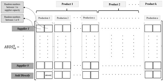
Figure 3.
Visual depiction of the chromosomal for ABDS variation.

Figure 4.
Illustration of the chromosome for the variable ABDA.

Figure 5.
Diagrammatic depiction of the chromosome of the ABDC variable.
3.3.3. Crossover Operators
In addition to creating a new solution space, the crossover operator produces offspring or new solutions between chromosomal pairs that mate. Initially, a random number between 1 and 4 is generated. Next, a chromosome or chromosomes is selected.
In the present study, three distinct crossover operators were considered to mate the chromosomal pairs to prevent permutation. Figure 6 illustrates these processes in a graphical manner, where the chromosome pairs were randomly selected with equal probability.
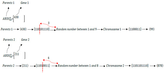
Figure 6.
Crossover representation sample.
3.4. Case Study and Data Collection
Malaysia is a country rich in fossil fuels and renewable energy resources. In terms of fossil resources, Malaysia holds 3.7 million barrels of oil (which accounts for 0.2% of the global share) and 38.5 trillion cubic feet of natural gas (which accounts for 0.6% of the worldwide share) [88]. Among all renewable forms, biomass is the only item that can be substituted for fossil fuels to produce different products, such as energy, materials, and chemicals. Substitution is reasonable; Malaysia’s major oil fields have experienced a significant decline in production capacity, and the country has abundant biomass resources [89].
The primary biomass source in Malaysia is palm oil. The country has 5 million hectares of palm fields, which produce approximately 93 million tons of palm oil [90]. Palm kernel and crude palm oil, which are critical raw materials for obtaining different basic oleochemicals and biodiesel, are generated after harvesting oil palm fruit. The palm oil industry also produces considerable amounts of agricultural waste (biomass), including palm oil trunks and fronds, palm oil mill effluent, empty fruit bunch (EFB), palm kernel shell, and palm mesocarp fiber. Zahraee et al. [89] reported that around 230 kg of EFBs are produced from each ton of processed oil palm fresh fruit bunch.
EFBs are inexpensive biomass resources that can be used to generate various products. The Malaysian government supports the use of biomass to produce value-added products and generate bioenergy through strategies and policies, such as the National Renewable Energy Policy, the National Biomass Strategy 2020, and the “1 Malaysia Biomass Alternative Strategy” [89]. According to the existing literature and commercialization activities, EFB is currently used to generate many different products, including briquette and pellet fuels, biogas, bio-oil, biosyngas, biohydrogen, biocomposite, biocompost, bioethanol, bioresin, activated carbon, and xylose [89]. Providing well-optimized BSC is a key factor in realizing this potential. The generation of oil palm products needs to be considered comprehensively and simultaneously. This study focuses on modeling an optimized SC for EFBs using Peninsular Malaysia as a case study.
The necessary data was gathered from several sources, including three case studies that the authors conducted in Malaysia, which included Johor, Pahang, and Perak, as well as previously published works in the field [89,90,91,92,93,94]. Furthermore, the Malaysian BSC was chosen to analyze its environmental performance due to its strong ties to sustainable development goals. The analyses focused on the intricate relationships between various suppliers, accounting for multiple modes of transportation (such as trucks, trains, and pipelines) and stages of production. Supplier selection is aided by these measurements of emissions produced by raw material supply systems.
3.5. Mathematical Model Development of BSC
Figure 7 illustrates the superstructure developed in this study, including the processing and storage facilities and sequences. The assumption is that each storage point is located within its facility.
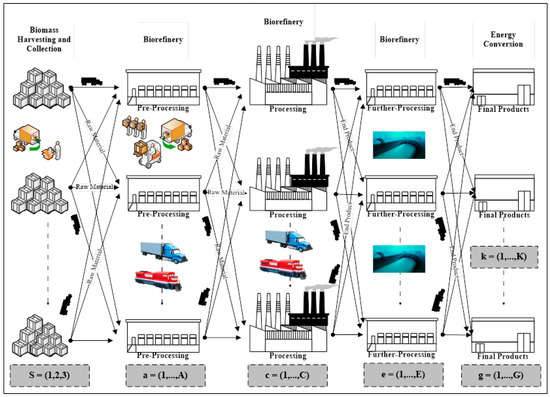
Figure 7.
Schematic view of EFB’s BSC.
Economic, environmental, and social performance is considered when developing the mathematical model of the ideal BSC. The profit realized from product sales is less than the total cost. Therefore, as seen below, the objective function of the optimization model aims to minimize environmental emissions while maximizing overall profit using Equation (1), which is equal to the (income − costs).
Reduce emissions by minimizing total emissions from production and transportation (see Equation (2))
Costs are the total expenses for biomass raw materials, delivery, production, and emissions from delivery and production, and income is the sales of goods. Consequently,
Profit = Total sale − raw material cost − delivery cost − production cost − emission cost from delivery − emission cost from production (see Equation (1)).
The terms mentioned above, such as the production and conversion factors’ CO2 emissions, the transportation process’s CO2 emissions, and the production cost factors’ CO2 emissions, all require information or parameters. The fixed costs, which include the capital costs, and the variable costs, which include the operational costs, are constants for various modes of transportation (such as trucks and trains). To calculate transportation costs, these components are multiplied at the mass flow rate after transportation costs are stated in dollars per tonne. This study considers a truck (distance > 100 km) and a train (distance < 100 km) as the preselected vehicles for solid biomass feedstock. Conversely, pipeline transportation is used for gaseous or liquid products. When producing a single unit of goods, the production cost factor (in US dollars ($)) is calculated, which includes the equipment’s capital and operational expenses. The mass flow rate in the BSC was multiplied by the emission factors for the selected transportation mode.
Production-related CO2 emission parameters were derived from prior research and other life cycle assessments [89]. As a standardized international unit of measurement, the CO2 equivalent (CO2e) was taken into consideration for transportation and manufacturing emission factors. A cost of $40 was allocated for each tonne of CO2e as the cost of the emission treatment [4]. The conversion factor in manufacturing facilities is defined as the raw material flow ratio from the inlet to the outlet. Using Google Maps and prior research, the separations between the two processing plants were measured. It should be mentioned that the cost of biomass raw material is $6 per tonne [84].
Table 3, Table 4, Table 5 and Table 6 provide all formula definitions, parameters, variables, and indexes required for the mathematical model. Equations (1)–(34) define the mathematical model, including goal functions, variable computations, and restrictions.
Table 3.
List of indexes.
Table 4.
List of parameters.
Table 5.
List of variables.
Table 6.
Definitions of formulas.
Model Validation
Mathematical model validation primarily determines how a computer model accurately represents the real world from the perspective of its intended application in a certain situation. This validation was performed by comparing the values predicted by a certain model with those obtained from experiments. At the initial step of the validation process, this study considered a small size of the proposed distribution network containing two suppliers , three production facilities level 1 , two production facilities at level 2 , two production facilities at level 3 , two production facilities at final level with two types of products . As explained earlier, the blending of EFBs was assumed to satisfy the supply requirements of pre-processing facilities. Table 7 presents the parameters and values of the developed model.
Table 7.
List of parameters and values of the GAMS model.
To validate the proposed model, the optimization model was validated in GAMS 36.2.0 using CPLEX 20.1.0.1 as the solver. The solution was then operated on an AMD A10-4600 M APU processor, which consisted of 6 sets, 4 scalars, 8 parameters, 29 single equations, and 29 variables. It took 1.578 s to solve the problem. According to the results given in Table 8, the proposed model was validated. For the given parameters, the minimum cost was found to be $2560 million per year. Table 8 shows the optimal production levels for all products, which used 3 million, 2 million, and 1.8 million tonnes per year of biomass feedstock for three suppliers. The total biomass production at each storage location is 1,690,106 and 2,400,762 tonnes per year.
Table 8.
Results of the GMAS model.
4. Results and Discussion
4.1. Results of NSGA-II and MOPSO
Two distinct examples of a bi-objective sustainable BSC optimization problem were solved using the NSGA-II and MOPSO algorithms, considering the pillars of social, environmental, and economic challenges. Two examples for the chosen case study were conducted to obtain numerous Pareto Solutions (PS). Table 9 displays the index values for each sample.
Table 9.
Index values for two examples.
Two distinct PSs were obtained from the results after the model was run. The PSs for the two environmental and economic goals achieved using NSGA-II and MOPSO are displayed in Figure 8. It is evident that there is a trade-off between environmental and economic goals. The largest amount of emissions is included in the maximum profit, which is equal to $7000 million. Profit decreases by over 40% to achieve the lowest possible environmental emissions. The same scenario occurs for the second example, which includes more BSC facilities. Figure 8 also shows the results of two algorithms: the maximum profit of BSC and the total emissions in each generation of the Pareto solution for the second example. As can be seen, the extended example achieves a better target value. Furthermore, Figure 9 demonstrates that the maximum economic objective is equal to $13,500 million, with the highest emissions. The environmental objective decreased to nearly 50%, thereby achieving 50% less profit. The developed model and proposed algorithms were implemented for four more examples to test the model, as shown in Figure 10.
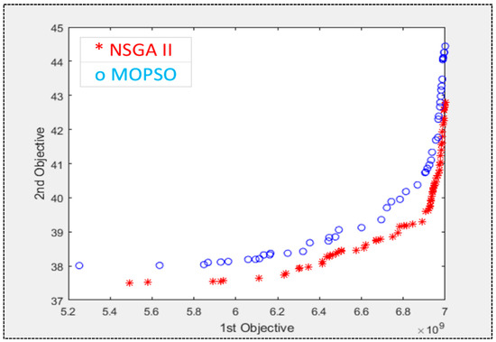
Figure 8.
Pareto Solutions of NSGA-II vs. MOPSO (example 1).
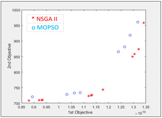
Figure 9.
Pareto solutions of NSGA-II vs. MOPSO (example 2).
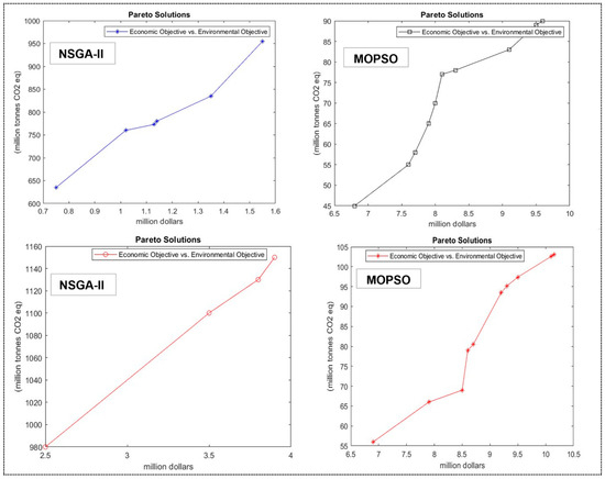
Figure 10.
Pareto solutions of NSGA-II vs. MOPSO.
In addition, five unique responses (each showcasing a particular quality of a solution attained by NSGA-II and MOPSO) were identified and used in the experiments to assess the efficacy of both algorithms. The identified responses are as follows: (1) CPU time; (2) Number of Pareto Solutions (NPS); (3) Mean Ideal Distance (MID); (4) Spacing (S); and (5) Maximum Spread (MS) [58]. The CPU times for the two runs of the NSGA-II results were 697.86 and 2125.90 s, and those for the MOPSO results were 391.76 and 1148.00 s, respectively. The proposed MOPSO algorithm can find a solution in less CPU time, as illustrated in Figure 11.
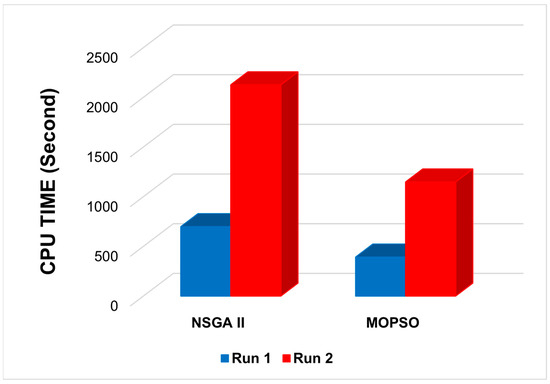
Figure 11.
CPU time of NSGA-II vs. MOSPSO.
In addition, five unique responses (each showcasing a particular quality of a solution attained by NSGA-II and MOPSO) were found and used in the experiments to assess the efficacy of both algorithms. The identified responses are as follows: (1) CPU time; (2) Number of Pareto Solutions (NPS); (3) Mean Ideal Distance (MID); (4) Spacing (S); and (5) Maximum Spread (MS) [58]. The CPU times for the two runs of the NSGA-II results are equal to 697.86 and 2125.90 s, and for MOPSO results, which are 391.76 and 1148.00 s, respectively. The MOPSO algorithm can find a solution in less CPU time, as shown in Figure 11.
According to Figure 12, most of the comparison results demonstrate that the NSGA-II method can find more PS for both examples, equal to 79 and 12, respectively. The proposed MOPSO algorithm generated 44 and 8 NPSs for the same examples.
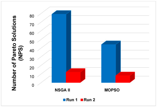
Figure 12.
Number of Pareto solutions in NSGA-II vs. MOSPSO.
Regarding the MID parameter, the NSGA-II method has less MID, for example, run 1, with fewer types of products, production facilities, and transportation modes compared to the same condition solved by the MOPSO algorithm (Figure 13). However, with the highest number of products, manufacturers, and transportation types, MOPSO has a lower and better MID than NSGA-II. In contrast, Figure 14 shows that NSGA-II, with the highest number of indexes, has less S (126,839) than MOPSO (681,860), as shown in Example 2. However, MOPSO delivers better S results—for example, 1.
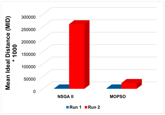
Figure 13.
Mean Ideal Distance for NSGA-II vs. MOSPSO.

Figure 14.
Spacing for NSGA-II vs. MOSPSO.
The MS parameter of the MOPSO algorithm is higher than that of NSGA-II in the second example, as shown in Figure 15. This can prove MOPSO’s aptitude for solving models with higher indexes. For the first case, the MS parameters were 454,540 for MOPSO and 487,960 for NSGA-II. Considering these findings, TOPSIS was used in the following phase to compare the parameters and select the superior algorithm by applying the TOPSIS criteria.

Figure 15.
Maximum Spacing Spread for NSGA-II vs. MOSPSO.
4.2. Implementation of the TOPSIS Method
The two-objective optimization results and TOPSIS are used to identify the optimal trade-off solutions. First, the two-objective optimization problems were solved to examine the optimum output under various variable conditions. This helps find the trade-off optimum design points from the standpoint of all the two objective functions simultaneously. Table 10 and Table 11 show the values and means of the performance parameters for each sample obtained using NSGA-II and MOPSO.
Table 10.
Summary of performance parameters and Mean results for NSGA-II.
Table 11.
Summary of performance parameters and Mean results for MOPSO.
In the next step, TOPSIS is applied to rank the given alternatives of PS obtained from NSGA-II and MOPSO developed by Hwang and Yoon [95]. In general, TOPSIS explores the positive ideal solution () and the negative ideal solution (). Then, it searches the Pareto set to identify the best compromise solution, which is the closest to and the farthest from , based on the objective weights allocated by the decision-maker. One of the most important steps in TOPSIS analysis is determining the. Several approaches can be used to calculate these weights, including the analytical hierarchy process (AHP), RANking COMparison (RANCOM), and direct expert assignment. The advantage of the AHP is that it can systematically derive weights via pairwise comparisons, which captures the relative importance of criteria. On the other hand, it requires careful judgment and consensus among decision-makers, which can be subjective and time-consuming [96]. In contrast, the RANCOM method provides an alternate weight determination method. To reduce subjectivity and bias in weight assignment, RANCOM employs randomization techniques to generate weights using random numbers. This approach is useful when determining the importance of the objective criteria is challenging or when resource limitations or a lack of agreement make traditional approaches like AHP impracticable. Ultimately, the method of choice should fit the particular context and objectives of the decision-making process, striking a balance between the necessity of systematic analysis and the useful factors of solution robustness and weight determination [91]. In this study, the weights were derived from expert knowledge.
In the following, the steps taken by TOPSIS to determine the best compromise solution are briefly described:
- (1)
- Input matrix , where the element is the objective value of the ith alternative (i.e., A is composed of the Pareto solutions).
- (2)
- Calculating the normalized rating according to the Equation (35). The vector normalization method is used in this method. The data processing logic is based on the Euclidean distance (second-order torque), so the vector method (Euclidean norm) is used. The vector method, unlike the simple linear normalization method, is performed as follows:
Equations (36)–(40) are used to calculate the as follows:
- (3)
- Constructing the weighted normalized values using the following Equation (41):
Table 12 summarizes the values for and .
Table 12.
Values of and .
In the next step, Equations (43)–(47) are used to calculate the as follows:
- (4)
- Equations (48) and (49) are used to find and as follows, where stands for a set of benefit attributes; note that larger values indicate better performance—for instance, the amount of production for a factory. signifies a set of cost attributes; remember that smaller values here indicate better performance, for example, the number of employees in a factory.
Table 13 shows the results of and for NSGA-II and MOPSO for two examples.
Table 13.
Values of and for NSGA-II and MOPSO.
- (5)
- Equations (50) and (51) are used to define the distance measure over each criterion to both ideal () and nadir (). Equations (52)–(55) demonstrate the calculations for and for NSGA-II and MOPSO.
- (6)
- In the last step of the calculations, Equation (56) is used to measure relative closeness for each Pareto solution as follows:
Equations (57) and (58) show the value of for NSGA_II and MOPSO as follows:
- (7)
- Finally, the best compromise solution whose relative closeness is the closest to 1 is selected.
According to the results, the MOPSO algorithm is closer to 1, demonstrating the MOPSO’s superiority compared with the NSGA-II algorithm. However, the NSGA-II algorithm could find more PS values when solving the BSC problem.
4.3. Sensitivity Analysis
A sensitivity analysis was performed to assess the uncertainties. Selling price, production cost, and demand were selected for the sensitivity analysis. The changes in these parameters were calculated by classifying them into three scenarios (Table 14). Both the original selling price and production cost factor were increased to 50%, and demand was set until a 10% increase. The first scenario shows that by increasing 10% of the selling price and cost by 2% demand, profit will increase, and the environmental objective will decrease by 15% (Figure 16). However, in the second scenario, profit will be reduced by 0.5%, and environmental objectives will be reduced by 35%. Figure 16 also shows that there should be a 10–30% increase in sales and cost to meet 2–8% demand.
Table 14.
Summary of scenarios.
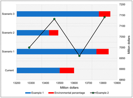
Figure 16.
Sensitivity analysis results.
4.4. Discussion
Assessing the financial viability of using oil palm EFB as a renewable feedstock for the production of materials, chemicals, and energy can be made easier using an ideal BSC. The prerequisite steps that should be taken to achieve the optimum BSC are presented; that is, steps that can be applied to various types of biomass feedstock and products. Three sustainability factors—economic, environmental, and social variables—were incorporated into the suggested model for use in tactical, operational, and strategic decision-making. It also helps determine optimal assignments for transportation modes by classifying processing routes and products according to their states (liquid, solid, or gas). Furthermore, the model considered environmental emissions and emissions costs from transportation and production activities.
Numerous significant trade-off points between objective functions were discovered due to this optimization. Such a MOO of profit and emissions could reveal significant design trade-offs between competing objective functions, which is difficult to find in any other way. The optimization results also consider the trade-off between profit and emissions considering economic and environmental concerns.
Note that the key advantage of the models proposed in this paper is that they can integrate strategic and tactical planning while considering the dynamic nature and operational limitations of SCs. Moreover, the developed models simultaneously considered the three pillars of sustainability. The MOO model presented in this study is the first application of BSCs that has combined simulation modeling and mathematical programming to address the complex problems typically associated with SCs. The developed multi-objective mathematical optimization model is also the first model that simultaneously integrates the economic, environmental, and social sustainability pillars of the BSC. Implementing two main evolutionary algorithms (NSGA-II and MOPSO) using the TOPSIS approach is another significant contribution that has not previously received attention in the BSC-planning literature. The mathematical optimization and simulation components of the proposed models were developed independently in the current paper. In addition, they are applied to similar case studies individually or together. Based on biomass and product types, adaptations to the simulation and optimization models may be needed. However, the general structure of the mathematical and dynamic simulation models is applicable to other cases without limitations. The case studies included substantial amounts of data regarding both bioenergy and biofuel production’s technical and economic aspects. Future research can use these data efficiently and effectively.
According to examples 1 and 2, the maximum profits are $13,500 million and $7000 million, respectively, which includes the most significant emissions. The optimization approach’s outcomes showed. The expanded example reduces 40% in profit to obtain the lowest possible emissions from manufacturing and transportation in BSC, which results in a better goal value. Furthermore, the performance of both methods was evaluated using five performance parameters. In comparison to NSGA-II, the nest CPU time associated with the MOPSO algorithm was 697.86 and 2125.90 s for each sample, respectively. Furthermore, the results demonstrate that compared to the MOPSO algorithm, the NSGA-II algorithm generated more Pareto solutions. Finally, several trade-off optimal design points were identified and subsequently presented using the TOPSIS approach to analyze the optimization algorithm solutions derived from the two objective problems. The outcomes demonstrated that MOPSO was better than NSGA-II; nevertheless, NSGA-II had a greater PS. These engine map points can be used by designers to improve performance.
Nevertheless, the PSO approach and NSGA-II are evolutionary algorithms that can result in nonconvergent, excessively high computational costs and suboptimal solutions. Further research could be conducted in this area to develop generation-algorithm-based multiobjective solution methods that are effective in reducing operating costs and gas emissions, such as the weighted sum technique and the ε-constraint method [97]. Researchers can run extensive simulations using (a Python library for multi-criteria decision-making (PYMCDM) to examine how SPOTIS functions in various weighting scenarios, particularly emphasizing how well it can reduce or eliminate rank reversal effects. In a similar vein, decision-making software platforms are interactive. It offers intuitive user interfaces for sensitivity testing and decision outcome visualization, which can improve the dependability and transparency of comparison studies between SPOTIS and alternative techniques.
In conclusion, incorporating interactive decision-making software and PYMCDM into research would make it easier to thoroughly explore the potential benefits of preventing rank reversal and improving our knowledge of and ability to use SPOTIS in real-world decision-making situations.
5. Conclusions
To take into account the social, environmental, and economic pillars of sustainability, this study simultaneously addresses sustainable BSC optimization. Initially, the economic principle is examined to optimize revenue and reduce the environmental impact of production and transportation within the BSC. To tackle these problems, a single multi-objective mathematical model was created using MATLAB software (R2024a) and evolutionary algorithms—specifically, NSGA-II and MOPSO. The TOPSIS method was proposed and employed as a multi-criteria decision analysis tool to compare, investigate, and rank a set of alternative solutions based on pre-specified criteria between the NSGA-II and MOPSO algorithms. The developed model was tested using two examples for the Malaysian Palm Oil case study. GAMES validated and verified the mathematical model using a simple case study example to compare the results. According to examples 1 and 2, the maximum profits are $13,500 million and $7000 million, respectively, which includes the greatest emissions, the optimization approach’s outcomes show. The expanded example reduces 40% of profits to obtain the lowest possible emissions from manufacturing and transportation in BSC, which results in a better goal value. In addition, five performance parameters were used to evaluate the performance of both algorithms. The nest CPU time is related to the MOPSO algorithm and is equal to 697.86 and 2125.90 s for each example, respectively, compared to NSGA-II. The results also demonstrate that the NSGA-II algorithm produced more Pareto solutions than the MOPSO algorithm. Some trade-off optimum design points were finally specified and presented by applying TOPSIS to the optimization algorithm solutions obtained from the two objective problems. In addition, MOPSO was found to be more successful than NSGA-II, while the latter had a higher PS value. Designers can use the same points on the engine map to improve performance.
Several uncertainty sources, including biomass availability, transportation times, and bulk density, were incorporated into the model proposed in this study. In addition, despite being highly variable in real-life situations, biomass quality attributes (e.g., ash content and moisture content) were assumed to be fixed in this research. This can significantly influence the final results because variations in biomass quality can result in significant financial losses.
The following are some ways in which future research can resolve the uncertainty in other model parameters that were mentioned in this study:
- There is room to account for equipment failure, repair timeframes, biomass quality, product costs, and demand. To do so, it is essential to estimate the probability distribution functions for uncertain parameters and incorporate them into the developed model. This is particularly important when considering seasonality in biomass supply and demand.
- Biomass must be stored and appropriately inventoried to avoid disruption to production processes due to variations in biomass demand and supply. Despite the challenge that uncertainty often creates for the economic viability of forest-based BSCs, most studies on bioenergy and biofuel SC planning have concentrated on deterministic models, and only a few researchers have integrated uncertainties into their models. An important reason for this is the intricacy of commonly used techniques (e.g., stochastic programming) when incorporating uncertainties into modeling. Such methods usually result in designing models requiring considerable computational effort to solve complex problems, such as models incorporating different planning levels.
- Future studies should extend the proposed model by considering the stochastic behavior of the economic, environmental, and social planning associated with BSC. Eventually, the proposed model can be used together with inventory management and technological risks for each processing route in the SC model to estimate performance measures accurately. In addition, future investigations are suggested for advances in the field of sensitivity analysis, providing a new perspective on the simultaneous influence of changes in multiple values on the robustness of the MCDM result.
Author Contributions
Conceptualization, S.M.Z.; Methodology, S.M.Z.; Software, S.M.Z.; Formal analysis, S.M.Z.; Investigation, S.M.Z.; Data curation, S.M.Z.; Writing—original draft, S.M.Z.; Writing—review & editing, N.S. and P.S.; Supervision, N.S. and P.S. All authors have read and agreed to the published version of the manuscript.
Funding
This research received no external funding.
Data Availability Statement
The original contributions presented in the study are included in the article, further inquiries can be directed to the corresponding author.
Conflicts of Interest
The authors declare no conflict of interest.
References
- Zahraee, S.M.; Golroudbary, S.R.; Shiwakoti, N.; Stasinopoulos, P.; Kraslawski, A. Water-energy nexus and greenhouse gas–sulfur oxides embodied emissions of biomass supply and production system: A large scale analysis using combined life cycle and dynamic simulation approach. Energy Convers. Manag. 2020, 220, 113113. [Google Scholar] [CrossRef]
- Zahraee, S.M.; Shiwakoti, N.; Stasinopoulos, P. A review on water-energy-greenhouse gas nexus of the bioenergy supply and production system. Curr. Sustain. Renew. Energy Rep. 2020, 7, 28–39. [Google Scholar] [CrossRef]
- Zahraee, S.M.; Assadi, M.K. Applications and challenges of the palm biomass supply chain in Malaysia. ARPN J. Eng. Appl. Sci. 2017, 12, 5789–5793. [Google Scholar]
- Zahraee, S.M.; Shiwakoti, N.; Stasinopoulos, P. Application of geographical information system and agent-based modeling to estimate particle-gaseous pollutant emissions and transportation cost of woody biomass supply chain. Appl. Energy 2022, 309, 118482. [Google Scholar] [CrossRef]
- Zahraee, S.M.; Shiwakoti, N.; Stasinopoulos, P. Agricultural biomass supply chain resilience: COVID-19 outbreak vs. sustainability compliance, technological change, uncertainties, and policies. Clean. Logist. Supply Chain 2022, 4, 100049. [Google Scholar] [CrossRef]
- Zahraee, S.M.; Shiwakoti, N.; Stasinopoulos, P. Simulation Scenario Analysis of Operational Day to Day Storage System of Biomass Supply Chain for a Power Plant Case Study Based on Logistic Cost and Transportation Emissions. In Proceedings of the 2021 International Conference on Advances in Electrical, Computing, Communication and Sustainable Technologies (ICAECT), Bhilai, India, 19–20 February 2021; pp. 1–8. [Google Scholar]
- Zahraee, S.M.; Golroudbary, S.R.; Shiwakoti, N.; Stasinopoulos, P.; Kraslawski, A. Transportation system analysis of empty fruit bunches biomass supply chain based on delivery cost and greenhouse gas emissions. Procedia Manuf. 2020, 51, 1717–1722. [Google Scholar] [CrossRef]
- An, H.; Wilhelm, W.E.; Searcy, S.W. Biofuel and petroleum-based fuel supply chain research: A literature review. Biomass Bioenergy 2011, 35, 3763–3774. [Google Scholar] [CrossRef]
- Zahraee, S.M. Sustainable Biomass Supply Chain Optimization. Ph.D. Thesis, RMIT University, Melbourne, Australia, 2022. [Google Scholar]
- Zahraee, S.M.; Shiwakoti, N.; Stasinopoulos, P. Biomass supply chain environmental and socio-economic analysis: 40-Years comprehensive review of methods, decision issues, sustainability challenges, and the way forward. Biomass Bioenergy 2020, 142, 105777. [Google Scholar] [CrossRef]
- Giarola, S.; Bezzo, F.; Shah, N. A risk management approach to the economic and environmental strategic design of ethanol supply chains. Biomass Bioenergy 2013, 58, 31–51. [Google Scholar] [CrossRef]
- Bernardi, A.; Giarola, S.; Bezzo, F. Optimizing the economics and the carbon and water footprints of bioethanol supply chains. Biofuels Bioprod. Biorefin. 2012, 6, 656–672. [Google Scholar]
- Čuček, L.; Varbanov, P.S.; Klemeš, J.J.; Kravanja, Z. Total footprints-based multi-criteria optimisation of regional biomass energy supply chains. Energy 2012, 44, 135–145. [Google Scholar] [CrossRef]
- Santibañez-Aguilar, J.E.; Morales-Rodriguez, R.; González-Campos, J.B.; Ponce-Ortega, J.M. Stochastic design of biorefinery supply chains considering economic and environmental objectives. J. Clean. Prod. 2016, 136 Pt B, 224–245. [Google Scholar] [CrossRef]
- Sims, R. Good Practice Guidelines: Bioenergy Project Development & Biomass Supply; IEA Bioenergy: Paris, France, 2007. [Google Scholar]
- Zahraee, S.M.; Golroudbary, S.R.; Shiwakoti, N.; Stasinopoulos, P. Particle-Gaseous pollutant emissions and cost of global biomass supply chain via maritime transportation: Full-scale synergy model. Appl. Energy 2021, 303, 117687. [Google Scholar] [CrossRef]
- Winston, W.L.; Goldberg, J.B. Operations Research: Applications and Algorithms; Duxbury Press Boston: Duxbury, MA, USA, 2004; Volume 3. [Google Scholar]
- Alvarez-Benitez, J.E.; Everson, R.M.; Fieldsend, J.E. A MOPSO algorithm based exclusively on pareto dominance concepts. In Proceedings of the International Conference on Evolutionary Multi-Criterion Optimization, Guanajuato, Mexico, 9–11 March 2005; pp. 459–473. [Google Scholar]
- Dulebenets, M.A. A comprehensive evaluation of weak and strong mutation mechanisms in evolutionary algorithms for truck scheduling at cross-docking terminals. IEEE Access 2018, 6, 65635–65650. [Google Scholar] [CrossRef]
- Dulebenets, M.A.; Pasha, J.; Kavoosi, M.; Abioye, O.F.; Ozguven, E.E.; Moses, R.; Boot, W.R.; Sando, T. Multiobjective optimization model for emergency evacuation planning in geographical locations with vulnerable population groups. J. Manag. Eng. 2020, 36, 04019043. [Google Scholar] [CrossRef]
- Kavoosi, M.; Dulebenets, M.A.; Abioye, O.F.; Pasha, J.; Wang, H.; Chi, H. An augmented self-adaptive parameter control in evolutionary computation: A case study for the berth scheduling problem. Adv. Eng. Inform. 2019, 42, 100972. [Google Scholar] [CrossRef]
- Pasha, J.; Dulebenets, M.A.; Fathollahi-Fard, A.M.; Tian, G.; Lau, Y.-y.; Singh, P.; Liang, B. An integrated optimization method for tactical-level planning in liner shipping with heterogeneous ship fleet and environmental considerations. Adv. Eng. Inform. 2021, 48, 101299. [Google Scholar] [CrossRef]
- Rabbani, M.; Oladzad-Abbasabady, N.; Akbarian-Saravi, N. Ambulance routing in disaster response considering variable patient condition: NSGA-II and MOPSO algorithms. J. Ind. Manag. Optim. 2022, 18, 1035. [Google Scholar] [CrossRef]
- Zhao, C.; Zhou, Y.; Chen, Z. Decomposition-based evolutionary algorithm with automatic estimation to handle many-objective optimization problem. Inf. Sci. 2021, 546, 1030–1046. [Google Scholar] [CrossRef]
- Zhao, H.; Zhang, C. An online-learning-based evolutionary many-objective algorithm. Inf. Sci. 2020, 509, 1–21. [Google Scholar] [CrossRef]
- Gonela, V. Stochastic optimization of hybrid electricity supply chain considering carbon emission schemes. Sustain. Prod. Consum. 2018, 14, 136–151. [Google Scholar] [CrossRef]
- Sarker, B.R.; Wu, B.; Paudel, K.P. Modeling and optimization of a supply chain of renewable biomass and biogas: Processing plant location. Appl. Energy 2019, 239, 343–355. [Google Scholar] [CrossRef]
- Fattahi, M.; Govindan, K.; Farhadkhani, M. Sustainable supply chain planning for biomass-based power generation with environmental risk and supply uncertainty considerations: A real-life case study. Int. J. Prod. Res. 2021, 59, 3084–3108. [Google Scholar] [CrossRef]
- Durmaz, Y.G.; Bilgen, B. Multi-objective optimization of sustainable biomass supply chain network design. Appl. Energy 2020, 272, 115259. [Google Scholar] [CrossRef]
- Cao, J.X.; Zhang, Z.; Zhou, Y. A location-routing problem for biomass supply chains. Comput. Ind. Eng. 2021, 152, 107017. [Google Scholar] [CrossRef]
- Aboytes-Ojeda, M.; Castillo-Villar, K.K.; Roni, M.S. A decomposition approach based on meta-heuristics and exact methods for solving a two-stage stochastic biofuel hub-and-spoke network problem. J. Clean. Prod. 2020, 247, 119176. [Google Scholar] [CrossRef]
- Mitchell, C. Development of decision support systems for bioenergy applications. Biomass Bioenergy 2000, 18, 265–278. [Google Scholar] [CrossRef]
- Venema, H.D.; Calamai, P.H. Bioenergy Systems Planning Using Location–Allocation and Landscape Ecology Design Principles. Ann. Oper. Res. 2003, 123, 241–264. [Google Scholar] [CrossRef]
- Dunnett, A.; Adjiman, C.; Shah, N. Biomass to Heat Supply Chains: Applications of Process Optimization. Process Saf. Environ. Prot. 2007, 85, 419–429. [Google Scholar] [CrossRef]
- Ayoub, N.; Martins, R.; Wang, K.; Seki, H.; Naka, Y. Two levels decision system for efficient planning and implementation of bioenergy production. Energy Convers. Manag. 2007, 48, 709–723. [Google Scholar] [CrossRef]
- Celli, G.; Ghiani, E.; Loddo, M.; Pilo, F.; Pani, S. Optimal location of biogas and biomass generation plants. In Proceedings of the 2008 43rd International Universities Power Engineering Conference, Padova, Italy, 1–4 September 2008; pp. 1–6. [Google Scholar]
- Izquierdo, J.; Minciardi, R.; Montalvo, I.; Robba, M.; Tavera, M. Particle Swarm Optimization for the biomass supply chain strategic planning. In Proceedings of the 4th Biennial Meeting of International Congress on Environmental Modelling and Software: Integrating Sciences and Information Technology for Environmental Assessment and Decision Making, iEMSs 2008, Barcelona, Catalonia, 7–10 July 2008; pp. 1272–1280. [Google Scholar]
- López, P.R.; Galán, S.G.; Reyes, N.R.; Jurado, F. A method for particle swarm optimization and its application in location of biomass power plants. Int. J. Green Energy 2008, 5, 199–211. [Google Scholar] [CrossRef]
- Rentizelas, A.A.; Tatsiopoulos, I.P.; Tolis, A. An optimization model for multi-biomass tri-generation energy supply. Biomass Bioenergy 2009, 33, 223–233. [Google Scholar] [CrossRef]
- Vera, D.; Carabias, J.; Jurado, F.; Ruiz-Reyes, N. A Honey Bee Foraging approach for optimal location of a biomass power plant. Appl. Energy 2010, 87, 2119–2127. [Google Scholar] [CrossRef]
- Han, S.-K.; Murphy, G.E. Solving a woody biomass truck scheduling problem for a transport company in Western Oregon, USA. Biomass Bioenergy 2012, 44, 47–55. [Google Scholar] [CrossRef]
- Singh, A.; Chu, Y.; You, F. Biorefinery Supply Chain Network Design under Competitive Feedstock Markets: An Agent-Based Simulation and Optimization Approach. Ind. Eng. Chem. Res. 2014, 53, 15111–15126. [Google Scholar] [CrossRef]
- Abriyantoro, D.; Dong, J.; Hicks, C.; Singh, S.P. A stochastic optimisation model for biomass outsourcing in the cement manufacturing industry with production planning constraints. Energy 2019, 169, 515–526. [Google Scholar] [CrossRef]
- Wang, J.-J.; Jing, Y.-Y.; Zhang, C.-F.; Zhao, J.-H. Review on multi-criteria decision analysis aid in sustainable energy decision-making. Renew. Sustain. Energy Rev. 2009, 13, 2263–2278. [Google Scholar] [CrossRef]
- Więckowski, J.; Sałabun, W.; Kizielewicz, B.; Bączkiewicz, A.; Shekhovtsov, A.; Paradowski, B.; Wątróbski, J. Recent advances in multi-criteria decision analysis: A comprehensive review of applications and trends. Int. J. Knowl.-Based Intell. Eng. Syst. 2023, 27, 367–393. [Google Scholar] [CrossRef]
- Askarifar, K.; Motaffef, Z.; Aazaami, S. An investment development framework in Iran’s seashores using TOPSIS and best-worst multi-criteria decision making methods. Decis. Sci. Lett. 2018, 7, 55–64. [Google Scholar] [CrossRef]
- Yeh, C.H. A problem-based selection of multi-attribute decision-making methods. Int. Trans. Oper. Res. 2002, 9, 169–181. [Google Scholar] [CrossRef]
- Chakraborty, S.; Yeh, C.-H. A simulation based comparative study of normalization procedures in multiattribute decision making. In Proceedings of the 6th Conference on 6th WSEAS International Conference on Artificial Intelligence, Knowledge Engineering and Data Bases, Corfu Island, Greece, 16–19 February 2007; pp. 102–109. [Google Scholar]
- Chakraborty, S.; Yeh, C.-H. Comparison based group ranking outcome for multiattribute group decisions. In Proceedings of the 2012 UKSim 14th International Conference on Computer Modelling and Simulation, Cambridge, UK, 28–30 March 2012; pp. 324–327. [Google Scholar]
- Hwang, C.; Yoon, K. Multiple Attribute Decision Making: Methods and Applications; Springer: New York, NY, USA, 1981. [Google Scholar]
- Gebreslassie, B.H.; Yao, Y.; You, F. Design under uncertainty of hydrocarbon biorefinery supply chains: Multiobjective stochastic programming models, decomposition algorithm, and a comparison between CVaR and downside risk. AIChE J. 2012, 58, 2155–2179. [Google Scholar] [CrossRef]
- Tong, K.; You, F.; Rong, G. Robust design and operations of hydrocarbon biofuel supply chain integrating with existing petroleum refineries considering unit cost objective. Comput. Chem. Eng. 2014, 68, 128–139. [Google Scholar] [CrossRef]
- Mas, M.D.; Giarola, S.; Zamboni, A.; Bezzo, F. Capacity planning and financial optimization of the bioethanol supply chain under price uncertainty. In Computer Aided Chemical Engineering; Pierucci, S., Ferraris, G.B., Eds.; Elsevier: Amsterdam, The Netherlands, 2010; Volume 28, pp. 97–102. [Google Scholar]
- Marufuzzaman, M.; Ekşioğlu, S.D.; Hernandez, R. Environmentally friendly supply chain planning and design for biodiesel production via wastewater sludge. Transp. Sci. 2014, 48, 555–574. [Google Scholar] [CrossRef]
- Wang, B.; Gebreslassie, B.H.; You, F. Sustainable design and synthesis of hydrocarbon biorefinery via gasification pathway: Integrated life cycle assessment and technoeconomic analysis with multiobjective superstructure optimization. Comput. Chem. Eng. 2013, 52, 55–76. [Google Scholar] [CrossRef]
- Yue, D.; Kim, M.A.; You, F. Design of Sustainable Product Systems and Supply Chains with Life Cycle Optimization Based on Functional Unit: General Modeling Framework, Mixed-Integer Nonlinear Programming Algorithms and Case Study on Hydrocarbon Biofuels. ACS Sustain. Chem. Eng. 2013, 1, 1003–1014. [Google Scholar] [CrossRef]
- Roni, M.S.; Eksioglu, S.D.; Cafferty, K.G.; Jacobson, J.J. A multi-objective, hub-and-spoke model to design and manage biofuel supply chains. Ann. Oper. Res. 2016, 249, 351–380. [Google Scholar] [CrossRef]
- Cambero, C.; Sowlati, T. Incorporating social benefits in multi-objective optimization of forest-based bioenergy and biofuel supply chains. Appl. Energy 2016, 178, 721–735. [Google Scholar] [CrossRef]
- Wheeler, J.; Páez, M.; Guillén-Gosálbez, G.; Mele, F.D. Combining multi-attribute decision-making methods with multi-objective optimization in the design of biomass supply chains. Comput. Chem. Eng. 2018, 113, 11–31. [Google Scholar] [CrossRef]
- Abdallah, T.; Farhat, A.; Diabat, A.; Kennedy, S. Green supply chains with carbon trading and environmental sourcing: Formulation and life cycle assessment. Appl. Math. Model. 2012, 36, 4271–4285. [Google Scholar] [CrossRef]
- Giarola, S.; Shah, N.; Bezzo, F. A comprehensive approach to the design of ethanol supply chains including carbon trading effects. Bioresour. Technol. 2012, 107, 175–185. [Google Scholar] [CrossRef]
- Zhu, Y.; Li, Y.; Huang, G. Planning carbon emission trading for Beijing’s electric power systems under dual uncertainties. Renew. Sustain. Energy Rev. 2013, 23, 113–128. [Google Scholar] [CrossRef]
- You, F.; Tao, L.; Graziano, D.J.; Snyder, S.W. Optimal design of sustainable cellulosic biofuel supply chains: Multiobjective optimization coupled with life cycle assessment and input–output analysis. AIChE J. 2012, 58, 1157–1180. [Google Scholar] [CrossRef]
- Yue, D.; Slivinsky, M.; Sumpter, J.; You, F. Sustainable Design and Operation of Cellulosic Bioelectricity Supply Chain Networks with Life Cycle Economic, Environmental, and Social Optimization. Ind. Eng. Chem. Res. 2014, 53, 4008–4029. [Google Scholar] [CrossRef]
- Bairamzadeh, S.; Pishvaee, M.S.; Saidi-Mehrabad, M. Multiobjective robust possibilistic programming approach to sustainable bioethanol supply chain design under multiple uncertainties. Ind. Eng. Chem. Res. 2015, 55, 237–256. [Google Scholar] [CrossRef]
- Miret, C.; Chazara, P.; Montastruc, L.; Negny, S.; Domenech, S. Design of bioethanol green supply chain: Comparison between first and second generation biomass concerning economic, environmental and social criteria. Comput. Chem. Eng. 2016, 85, 16–35. [Google Scholar] [CrossRef]
- Chávez, M.M.M.; Sarache, W.; Costa, Y. Towards a comprehensive model of a biofuel supply chain optimization from coffee crop residues. Transp. Res. Part E Logist. Transp. Rev. 2018, 116, 136–162. [Google Scholar] [CrossRef]
- Tsao, Y.-C.; Thanh, V.-V.; Lu, J.-C.; Yu, V. Designing sustainable supply chain networks under uncertain environments: Fuzzy multi-objective programming. J. Clean. Prod. 2018, 174, 1550–1565. [Google Scholar] [CrossRef]
- Zahraee, S.M.; Maydanchi, M.; Shiwakoti, N.; Stasinopoulos, P. Global Biomass Supply Chain Resilience Optimization Based on Sustainability Pillars. In SDGs in the Asia and Pacific Region; Leal Filho, W., Ng, T.F., Iyer-Raniga, U., Ng, A., Sharifi, A., Eds.; Springer International Publishing: Cham, Switzerland, 2023; pp. 1–26. [Google Scholar] [CrossRef]
- Holland, J.H. Adaptation in Natural and Artificial Systems: An Introductory Analysis with Applications to Biology, Control, and Artificial Intelligence; MIT Press: Cambridge, MA, USA, 1992. [Google Scholar]
- Kennedy, J.; Eberhart, R. Particle swarm optimization. In Proceedings of the ICNN’95-International Conference on Neural Networks, Perth, WA, Australia, 27 November–1 December 1995; pp. 1942–1948. [Google Scholar]
- Dorigo, M.; Maniezzo, V.; Colorni, A. Ant system: Optimization by a colony of cooperating agents. IEEE Trans. Syst. Man Cybern. Part B 1996, 26, 29–41. [Google Scholar] [CrossRef] [PubMed]
- Kirkpatrick, S.; Gelatt, C.D.; Vecchi, M.P. Optimization by simulated annealing. Science 1983, 220, 671–680. [Google Scholar] [CrossRef]
- Meng, A.-B.; Chen, Y.-C.; Yin, H.; Chen, S.-Z. Crisscross optimization algorithm and its application. Knowl.-Based Syst. 2014, 67, 218–229. [Google Scholar] [CrossRef]
- Talbi, E.-G. Metaheuristics: From Design to Implementation; John Wiley & Sons: Hoboken, NJ, USA, 2009; Volume 74. [Google Scholar]
- Deb, K.; Agrawal, S.; Pratap, A.; Meyarivan, T. A fast elitist non-dominated sorting genetic algorithm for multi-objective optimization: NSGA-II. In Proceedings of the International Conference on Parallel Problem Solving from Nature, Paris, France, 18–20 September 2000; pp. 849–858. [Google Scholar]
- Deb, K. Multi-objective optimisation using evolutionary algorithms: An introduction. In Multi-Objective Evolutionary Optimisation for Product Design and Manufacturing; Springer: Berlin/Heidelberg, Germany, 2011; pp. 3–34. [Google Scholar]
- Yang, X.-S. Nature-inspired optimization algorithms: Challenges and open problems. J. Comput. Sci. 2020, 46, 101104. [Google Scholar] [CrossRef]
- Reyes-Sierra, M.; Coello, C.C. Multi-objective particle swarm optimizers: A survey of the state-of-the-art. Int. J. Comput. Intell. Res. 2006, 2, 287–308. [Google Scholar]
- Sengupta, S.; Basak, S.; Peters, R.A. Particle Swarm Optimization: A survey of historical and recent developments with hybridization perspectives. Mach. Learn. Knowl. Extr. 2019, 1, 157–191. [Google Scholar] [CrossRef]
- Moore, J. Application of Particle Swarm to Multiobjective Optimization; Technical Report; Department of Computec Science and Software Engineering, Anburn University: Auburn, AL, USA, 1999. [Google Scholar]
- Coello, C.C.; Lechuga, M.S. MOPSO: A proposal for multiple objective particle swarm optimization. In Proceedings of the 2002 Congress on Evolutionary Computation. CEC’02 (Cat. No. 02TH8600), Washington, DC, USA, 12–17 May 2002; pp. 1051–1056. [Google Scholar]
- Tripathi, P.K.; Bandyopadhyay, S.; Pal, S.K. Multi-objective particle swarm optimization with time variant inertia and acceleration coefficients. Inf. Sci. 2007, 177, 5033–5049. [Google Scholar] [CrossRef]
- Liu, D.; Tan, K.C.; Huang, S.; Goh, C.K.; Ho, W.K. On solving multiobjective bin packing problems using evolutionary particle swarm optimization. Eur. J. Oper. Res. 2008, 190, 357–382. [Google Scholar] [CrossRef]
- Mirjalili, S.; Hashim, S.Z.M. A new hybrid PSOGSA algorithm for function optimization. In Proceedings of the 2010 International Conference on Computer and Information Application, Washington, DC, USA, 29 June 2010; pp. 374–377. [Google Scholar]
- Beheshti, Z.; Shamsuddin, S.M.H. CAPSO: Centripetal accelerated particle swarm optimization. Inf. Sci. 2014, 258, 54–79. [Google Scholar] [CrossRef]
- Luo, J.; Qi, Y.; Xie, J.; Zhang, X. A hybrid multi-objective PSO–EDA algorithm for reservoir flood control operation. Appl. Soft Comput. 2015, 34, 526–538. [Google Scholar] [CrossRef]
- MPOB. Overview of The Malaysian Oil Palm Industry 2019; MPOB: Selangor, Malaysia, 2020. [Google Scholar]
- Zahraee, S.M.; Golroudbary, S.R.; Shiwakoti, N.; Kraslawski, A.; Stasinopoulos, P. An investigation of the environmental sustainability of palm biomass supply chains via dynamic simulation modeling: A case of Malaysia. J. Clean. Prod. 2019, 237, 117740. [Google Scholar] [CrossRef]
- Ng, R.T.; Ng, D.K. Systematic approach for synthesis of integrated palm oil processing complex. Part 1: Single owner. Ind. Eng. Chem. Res. 2013, 52, 10206–10220. [Google Scholar] [CrossRef]
- Malaysian Palm Oil Board. Biomass Availability for 2016. Available online: http://bepi.mpob.gov.my/index.php/statistics/yield.html (accessed on 7 June 2024).
- Murillo-Alvarado, P.E.; Guillén-Gosálbez, G.; Ponce-Ortega, J.M.; Castro-Montoya, A.J.; Serna-González, M.; Jiménez, L. Multi-objective optimization of the supply chain of biofuels from residues of the tequila industry in Mexico. J. Clean. Prod. 2015, 108 Pt A, 422–441. [Google Scholar] [CrossRef]
- Zhang, Y.; Sun, W.; Wang, H.; Geng, A. Polyhydroxybutyrate production from oil palm empty fruit bunch using Bacillus megaterium R11. Bioresour. Technol. 2013, 147, 307–314. [Google Scholar] [CrossRef] [PubMed]
- Zheng, Y.; Zhao, J.; Xu, F.; Li, Y. Pretreatment of lignocellulosic biomass for enhanced biogas production. Prog. Energy Combust. Sci. 2014, 42, 35–53. [Google Scholar] [CrossRef]
- Hwang, C.-L.; Yoon, K. Methods for multiple attribute decision making. In Multiple Attribute Decision Making; Springer: Berlin/Heidelberg, Germany, 1981; pp. 58–191. [Google Scholar]
- Więckowski, J.; Kizielewicz, B.; Shekhovtsov, A.; Sałabun, W. RANCOM: A novel approach to identifying criteria relevance based on inaccuracy expert judgments. Eng. Appl. Artif. Intell. 2023, 122, 106114. [Google Scholar] [CrossRef]
- Li, Z.; Xu, Y.; Fang, S.; Wang, Y.; Zheng, X. Multiobjective coordinated energy dispatch and voyage scheduling for a multienergy ship microgrid. IEEE Trans. Ind. Appl. 2019, 56, 989–999. [Google Scholar] [CrossRef]
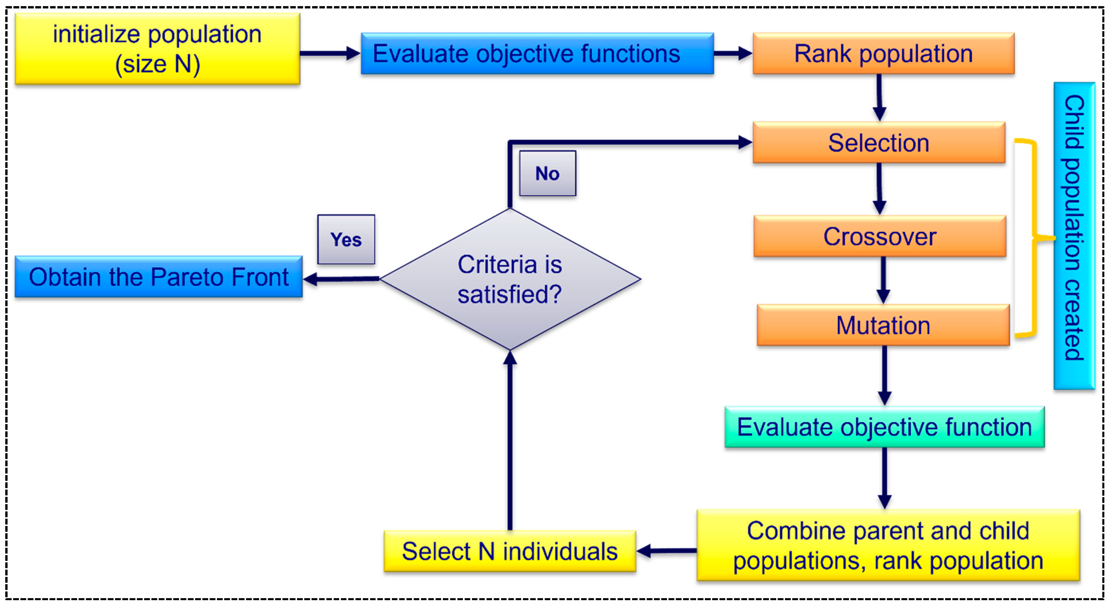
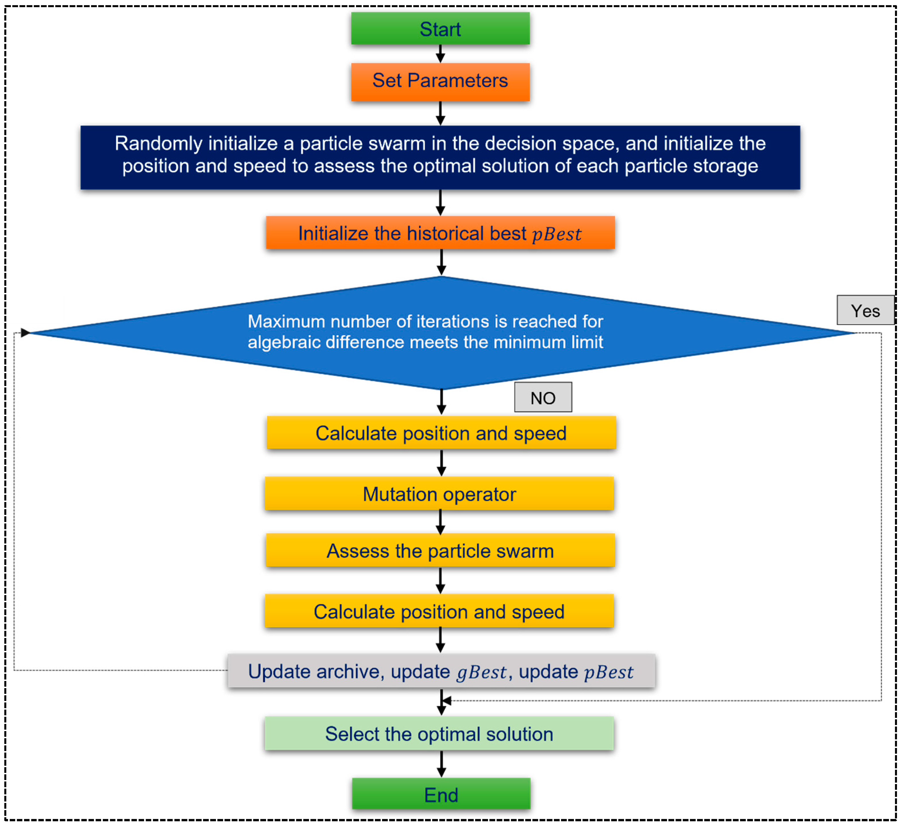
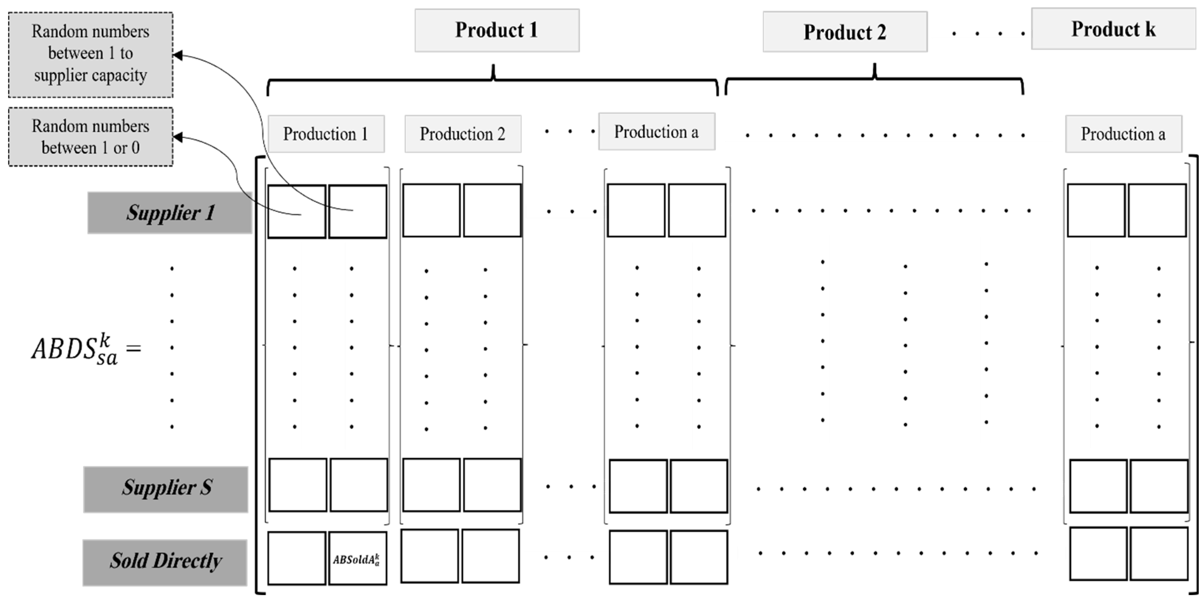
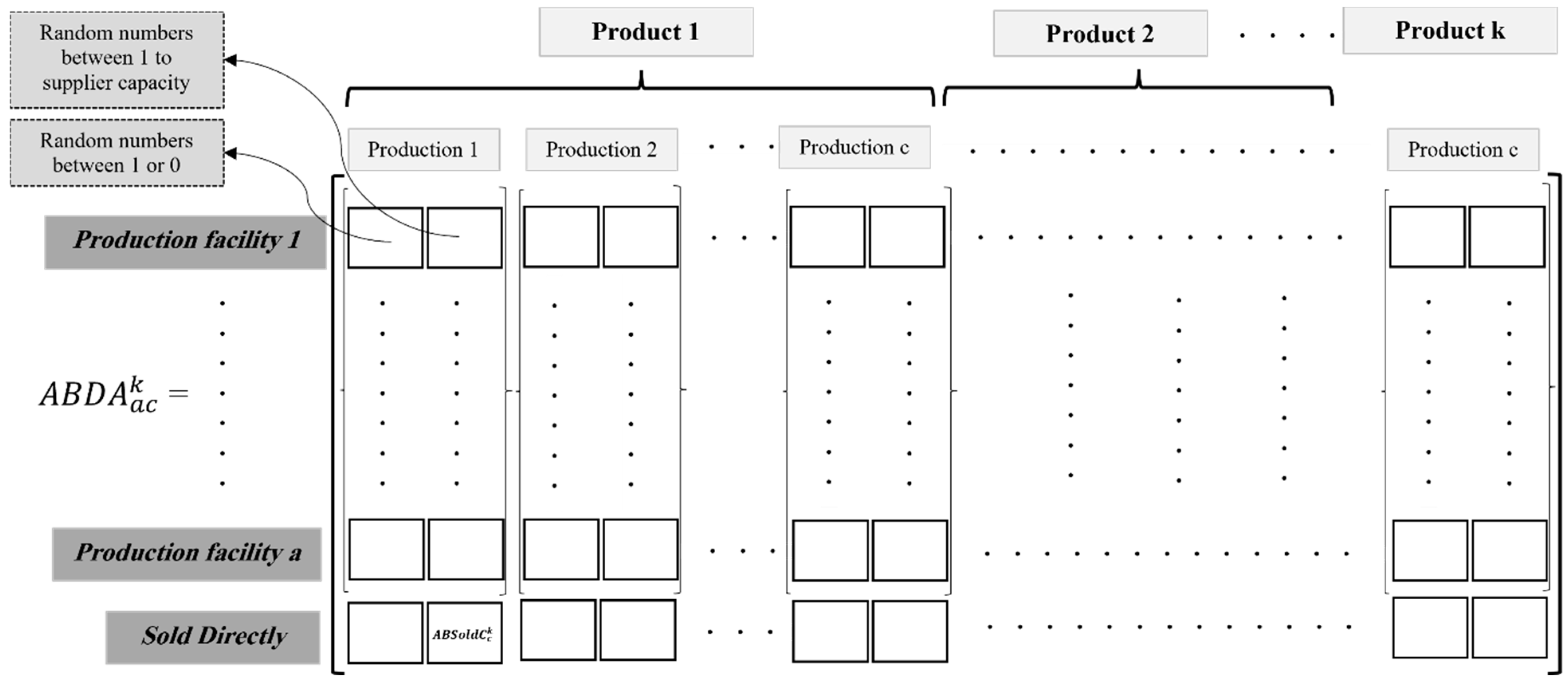
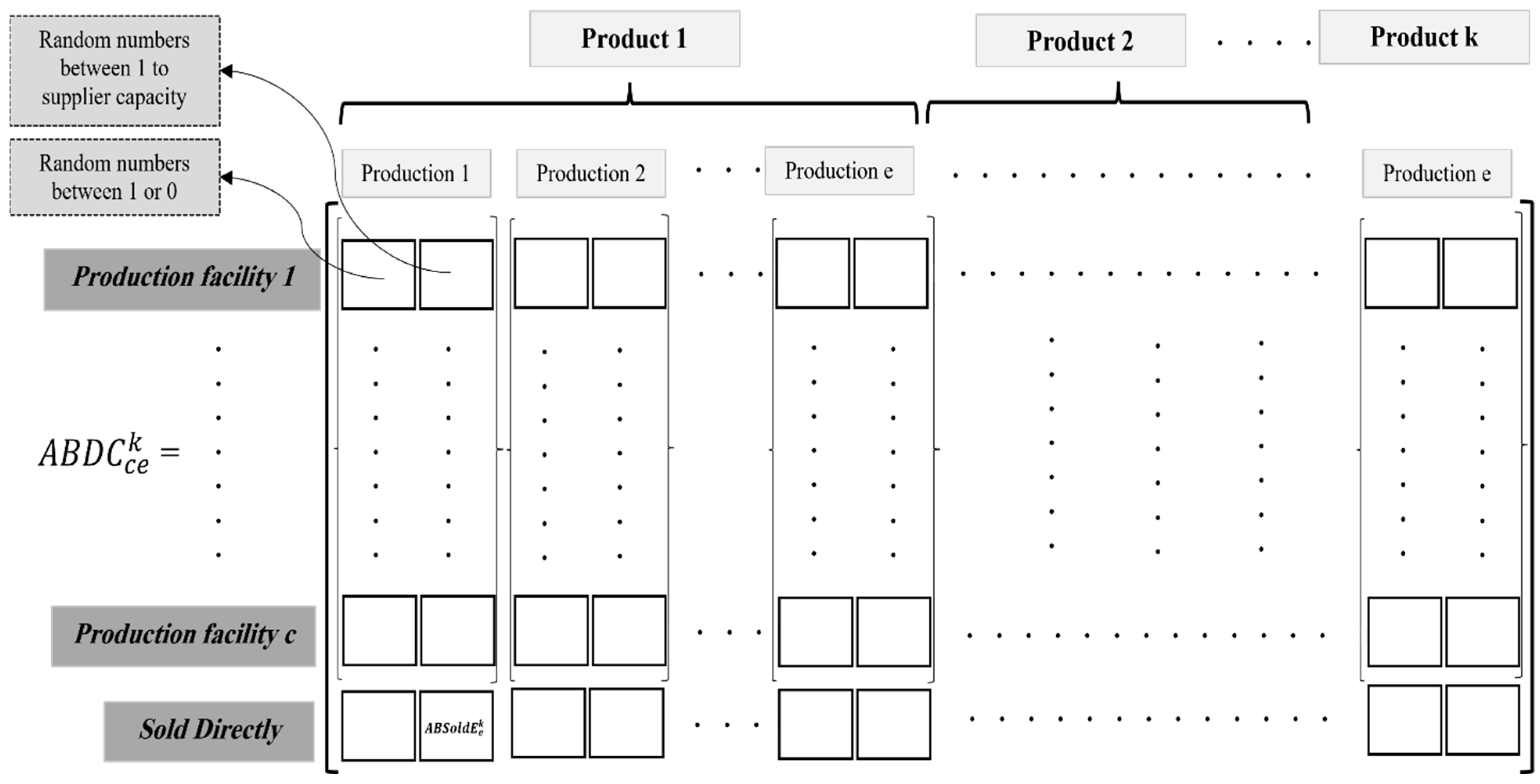
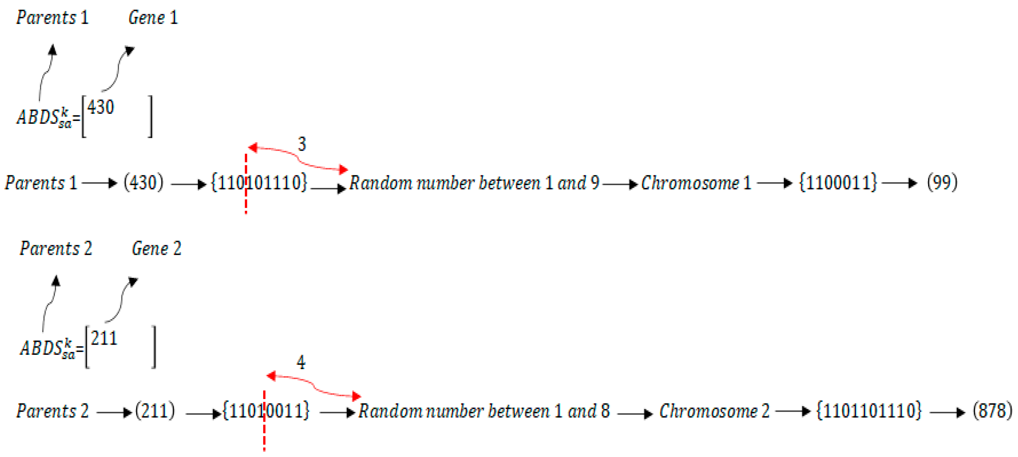
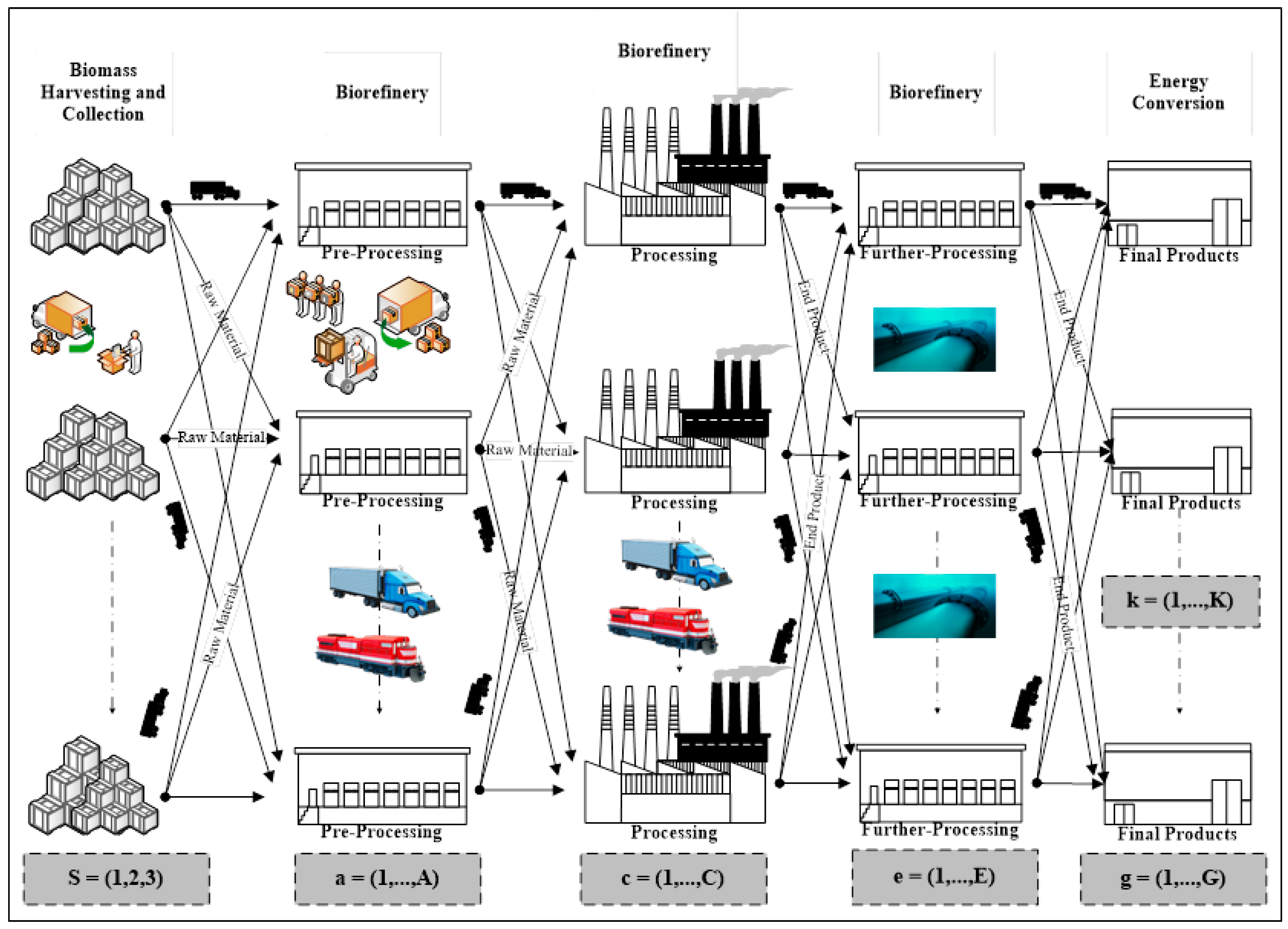
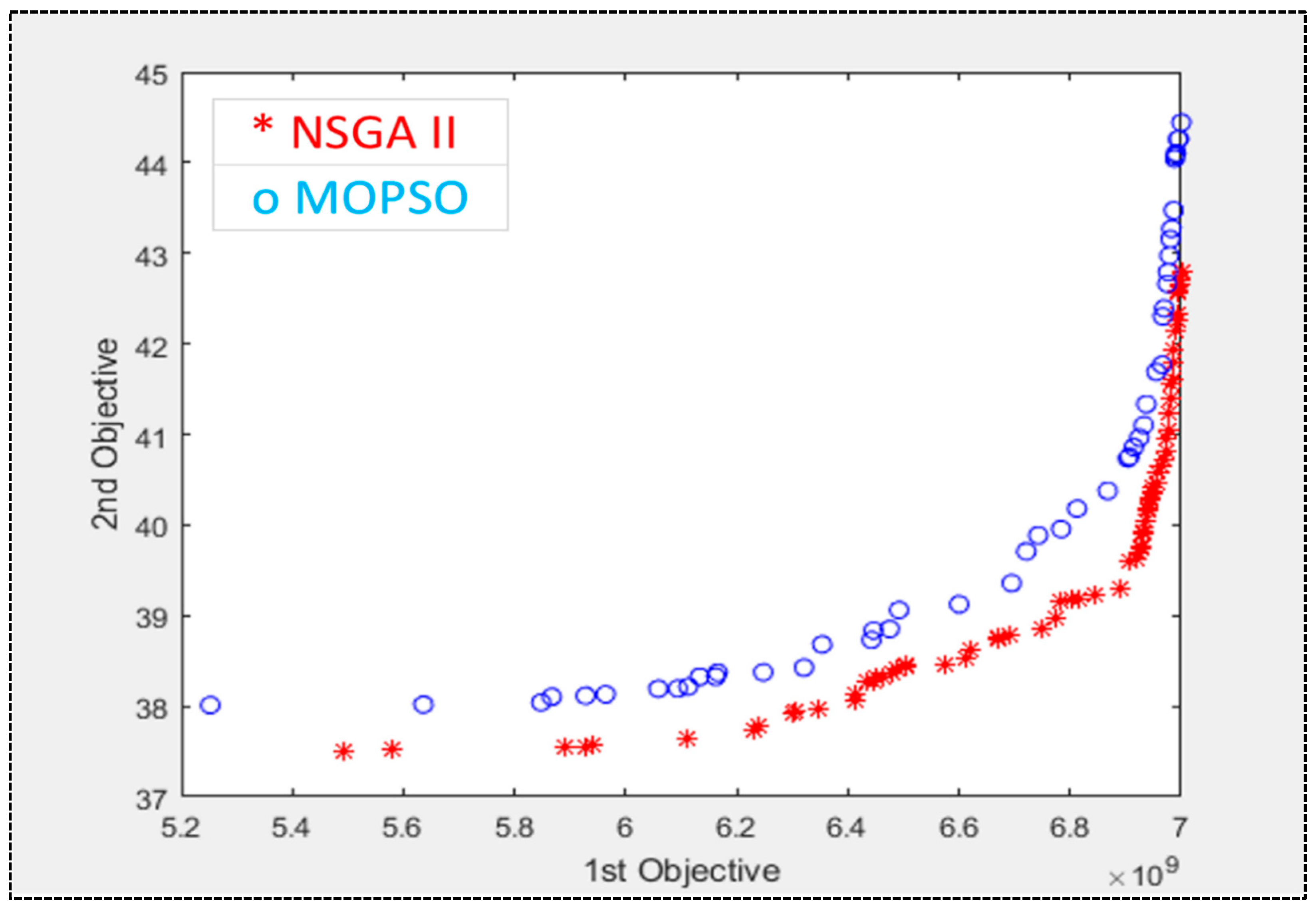

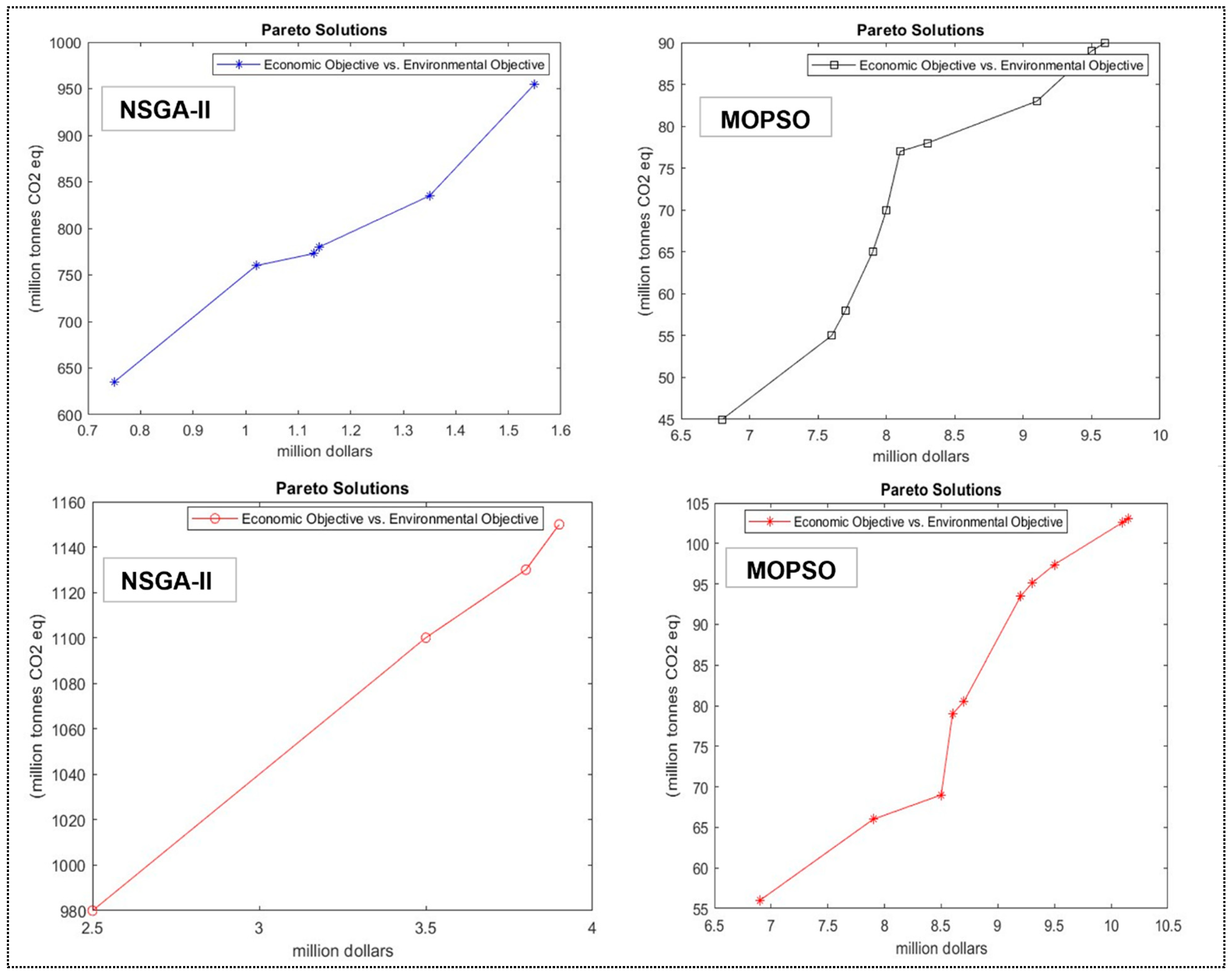


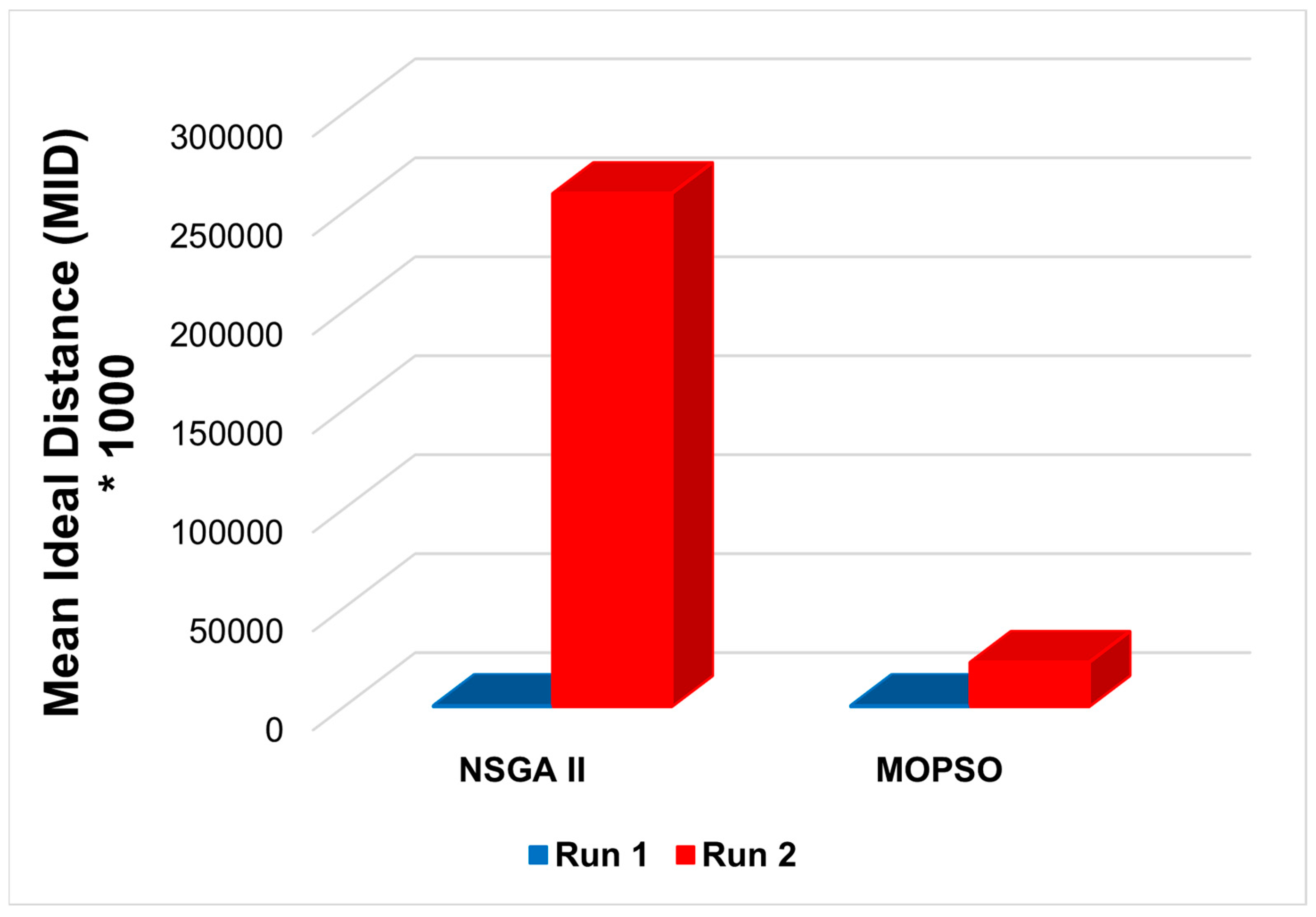
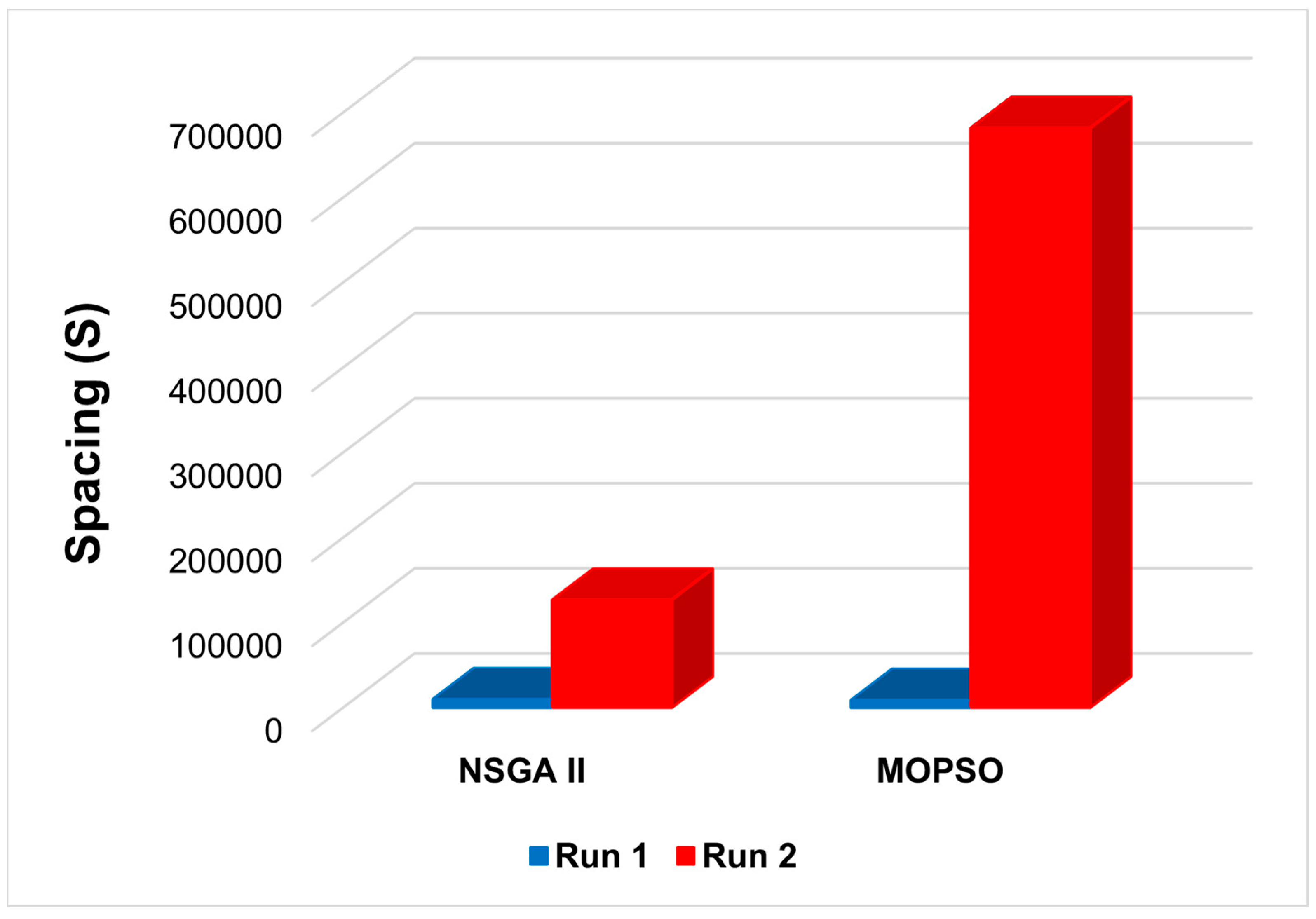
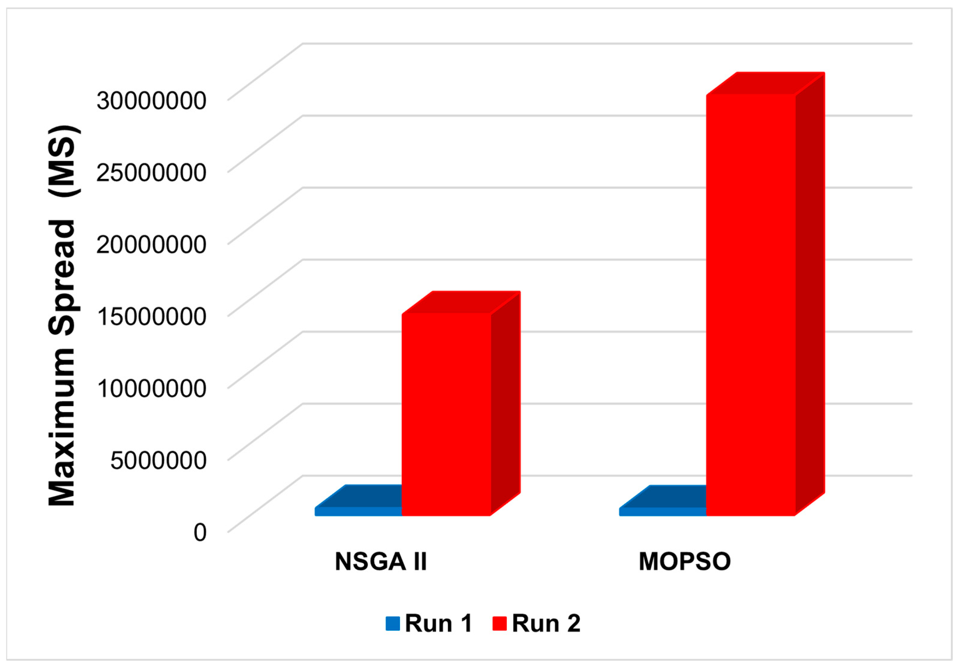
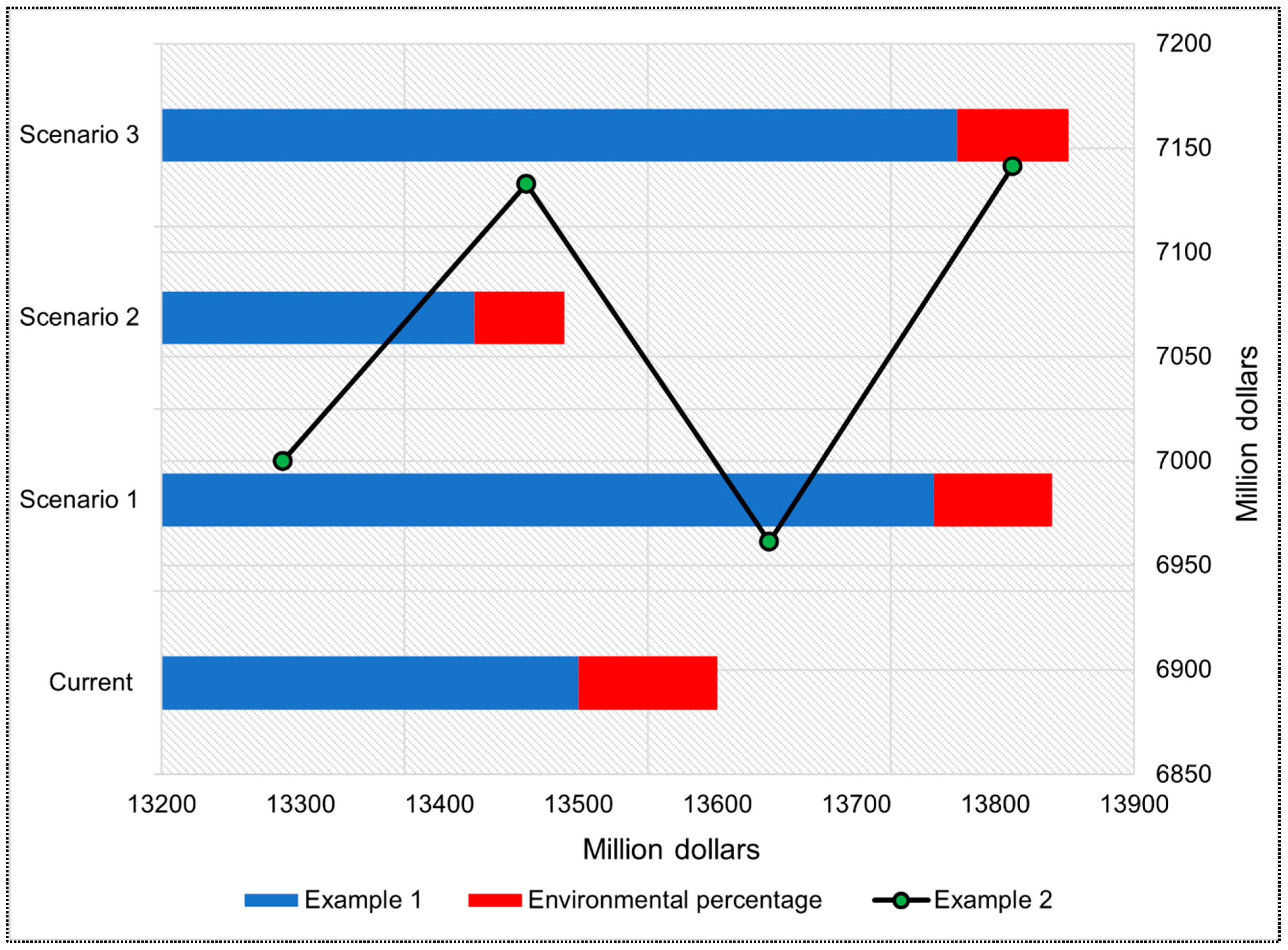
Disclaimer/Publisher’s Note: The statements, opinions and data contained in all publications are solely those of the individual author(s) and contributor(s) and not of MDPI and/or the editor(s). MDPI and/or the editor(s) disclaim responsibility for any injury to people or property resulting from any ideas, methods, instructions or products referred to in the content. |
© 2024 by the authors. Licensee MDPI, Basel, Switzerland. This article is an open access article distributed under the terms and conditions of the Creative Commons Attribution (CC BY) license (https://creativecommons.org/licenses/by/4.0/).