Hydrodynamic Performance of a Dual-Pontoon WEC-Breakwater System: An Analysis of Wave Energy Content and Converter Efficiency

Abstract

A dual-pontoon WEC-breakwater system is proposed to optimise space utilisation and reduce construction costs by integrating wave energy converters (WECs) with breakwaters. Previous parametric studies on the dimensions and layout of WECs have primarily used potential flow theories, often neglecting the viscous effects in wave–pontoon interactions. In this research, I employ a fully nonlinear viscous model, OpenFOAM^®, to address these limitations. I examine multiple parameters, including the gap width between the pontoons, the draft, and the structure breadth, to assess their impact on the functional performance of this hybrid system. Furthermore, I discuss the accurate hydrodynamic performance of waves interacting with multiple floating structures and explore how various parameters influence the dual-pontoon WEC-breakwater integrated system’s functionality. I discuss a novel analysis of the effective frequency bandwidth, considering both wave energy conversion efficiency and wave attenuation efficiency, to reflect the overall performance of the integrated system. This paper investigates wave–structure interactions and suggests optimisation strategies for the WEC-breakwater integrated system.

1. Introduction

With increasing global energy demand, environmental pollution, and the looming threat of climate change, there is an urgent need for reliable, affordable, and sustainable energy generation. Wave energy is a promising option in this context [1], offering vast storage potential that could meet global energy needs [2,3,4]. Wave energy converters (WECs) are deployed in coastal or offshore areas to harness this energy. However, the high costs associated with current WEC technology hinder its large-scale practical application [5]. A potential solution to this challenge is to share the construction costs of WECs with other functional structures [6].

Breakwaters, designed to protect coastlines by dissipating wave energy, are ideal for integration with WECs. Both structures are typically located in coastal and nearshore areas, and WECs can aid breakwaters by converting wave energy, thereby enhancing wave attenuation.

Several integrated WEC-breakwater system designs have been explored by researchers. Studies [7,8,9] have investigated systems combining oscillating water column (OWC)-type WECs with fixed-body breakwaters, where an air chamber within the breakwater drives an air turbine via oscillating water columns. Another study [1] examined a modified rubble-mound WEC-breakwater system with an overtopping reservoir that channels captured waves back to the sea through a turbine.

Fixed-body breakwaters can be prohibitively expensive in regions with high tidal ranges or deep waters. To address this, floating breakwaters integrated with WECs have been proposed. Research [10,11,12] has utilised flexible floating breakwaters (FFBs), where the relative motion of FFB bodies in waves generates energy through a power take-off (PTO) system.

Ning et al. [13] introduced a pile-restrained floating breakwater within an integrated WEC-breakwater system (hereafter WEC-B system), as shown in Figure 1. This system features a point absorber-type WEC with a floating pontoon restricted by vertical piles, allowing only heave motion. The heave motion drives a PTO system via a toothed rack and gear mechanism, simulating power generation. Experiments demonstrated that this WEC-B system effectively attenuates waves and extracts energy [13].

Further development of the WEC-B system led Ning et al. [14] to propose a dual-pontoon setup. Analytical studies indicated that dual pontoons improve performance over a single pontoon [14]. Recent advancements have explored asymmetric WEC geometries [15,16] and multiple degrees of freedom [17]. However, discussions on the relative dimensions and layout of dual pontoons have been limited, and the effects of flow viscosity have not been fully considered. The previous studies in [14] utilised linear potential flow theories that assume an inviscid, incompressible, and irrotational flow, thereby neglecting the effects of viscosity. These linear theories simplify the flow to linear behaviour, which limits their ability to capture complex flow phenomena such as vortex shedding and boundary layer separation. While suitable for initial design and analysis due to their high computational efficiency, they lack accuracy in representing real-world viscous effects. In contrast, this study incorporates a fully nonlinear viscous model that includes the effects of viscosity, providing a more realistic simulation of fluid–structure interactions. This model allows me to simulate complex phenomena such as vortex formation, boundary layer separation, and energy dissipation due to viscous effects, which is critical for understanding the impact on heave displacement and overall system efficiency. By capturing the formation and evolution of vortices, this viscous approach offers a detailed analysis of how these factors influence the performance of the WEC-B system. Additionally, the viscous model can accurately represent boundary layer phenomena, while linear potential flow theories cannot.

Computational fluid dynamics (CFD) based on the Navier–Stokes equations is employed to capture nonlinear wave–structure interactions and vortex evolution. With advances in computing technology, CFD tools are increasingly used in engineering design. OpenFOAM^® is a free, open-source C++ library for continuum-mechanics problems, widely applied in coastal and offshore engineering. Studies by Morgan et al. [18,19] validated OpenFOAM^® for coastal applications by accurately reproducing wave propagation over a submerged bar. Jacobsen et al. [20] enhanced OpenFOAM^® with wave generation and absorption methods. Chen et al. [21,22] demonstrated its accuracy in modelling nonlinear wave interactions and the roll motions of floating structures.

This paper validates the use of OpenFOAM^® for modelling interactions between waves and floating WEC devices through comparison with experimental data. The validated model investigates WEC-B system performance and configuration influences. OpenFOAM^®’s ability to represent vortex evolution aids in understanding how different parameters affect functional performance.

In summary, this study introduces several innovations that distinguish it from previous research. Firstly, unlike previous studies, this research fully incorporates the effects of flow viscosity using OpenFOAM^®, a fully nonlinear viscous model. This approach provides a more accurate representation of wave–pontoon interactions. Secondly, the study further optimises the WEC-B system by evaluating key parameters such as the gap width between pontoons, pontoon draft, and structure breadth. These parameters are systematically analysed to determine their impact on system performance. Lastly, the effective frequency bandwidth is introduced and discussed to reflect the overall functional performance of the integrated WEC-B system. This novel approach combines wave attenuation (KT) and wave energy extraction efficiency (CWR) to provide a comprehensive performance evaluation. These innovations contribute significantly to the existing body of research by addressing previously unexplored aspects and providing a more holistic understanding of the WEC-B system’s performance.

The paper is structured as follows. Section 2 details the numerical model. Section 3 describes the design of the numerical wave tank, test conditions, and mesh setup. Section 4 validates the numerical wave tank. Section 5 discusses the numerical results. Section 6 concludes the findings.

2. Numerical Model

2.1. Governing Equations

The interFOAM solver in OpenFOAM^® employs the Navier–Stokes equations to describe fluid motion. These are expressed as the mass conservation equation (Equation (1)) and the momentum equation (Equation (2)), derived from Newton’s second law:

$$\nabla ·\overrightarrow{U}=0,$$

(1)

$${\displaystyle \frac{\partial \rho \overrightarrow{U}}{\partial t}}+\nabla ·\left(\rho \overrightarrow{U}\overrightarrow{U}\right)-\nabla ·\left(\mu \nabla \overrightarrow{U}\right)-\rho \overrightarrow{\mathrm{g}}=-\nabla p-\overrightarrow{f_{\sigma }},$$

(2)

where $\overrightarrow{U}$ is the flow velocity vector, $\rho$ is the fluid density, $\mu$ is the dynamic viscosity, $\overrightarrow{\mathrm{g}}$ is the gravitational acceleration, p is the fluid pressure, and $\overrightarrow{f_{\sigma }}$ represents the surface tension effects, which are minor in civil engineering contexts. The unknowns in these equations are the three velocity components and the fluid pressure.

The pressure–velocity coupling is addressed using the PIMPLE algorithm, which combines the SIMPLE (Semi-Implicit Method for Pressure-Linked Equations) [23] and PISO (Pressure-Implicit Splitting Operator) [24] algorithms. The SIMPLE iterates to solve the pressure from the velocity components, while the PISO corrects the pressure–velocity relationship within the PIMPLE framework. To solve the Navier–Stokes equations, partial differential equations are integrated over the solution domain and time domain, then discretised into mesh cells and time steps. The values at mesh cell centroids represent different variables and properties. The Courant number [25] is used to ensure model stability and accuracy. The PIMPLE algorithm discretises the pressure and velocity equations into volume and surface integrals, which are then linearised using the appropriate schemes detailed in the OpenFOAM^® manual [26].

2.2. Free Surface Tracking

The volume of fluid (VOF) method in OpenFOAM^® is used to track the free surface’s shape and position. The VOF transport equation is represented as follows:

$${\displaystyle \frac{\partial \gamma }{\partial t}}+\nabla ·\left(\overrightarrow{U}\gamma \right)=0,$$

(3)

where $\gamma$ is the volume fraction (0 for air, 1 for water, and intermediate values for mixed cells). An additional convective term is included for sharper interface resolution. The velocity field, modelled by gas (${\overrightarrow{U}}_{\mathrm{g}}$) and liquid (${\overrightarrow{U}}_{\mathrm{l}}$) velocities, is a weighted average represented as $\overrightarrow{U}=\gamma {\overrightarrow{U}}_{\mathrm{l}}+(1-\gamma ){\overrightarrow{U}}_{\mathrm{g}}$. This results in a modified VOF transport equation:

$${\displaystyle \frac{\partial \gamma }{\partial t}}+\nabla ·\left(\overrightarrow{U}\gamma \right)+\nabla \left[{\overrightarrow{U}}_r\gamma \left(1-\gamma \right)\right]=0,$$

(4)

where ${\overrightarrow{U}}_r={\overrightarrow{U}}_{\mathrm{l}}-{\overrightarrow{U}}_{\mathrm{g}}$. In OpenFOAM^®, two immiscible fluids are treated as a single effective fluid with properties such as density and viscosity expressed as weighted averages:

$$\varphi =\gamma {\varphi }_{water}+(1-\gamma ){\varphi }_{air},$$

(5)

This method ensures that physical properties match those of each fluid in their respective regions and vary across the interface [27].

2.3. Wave Generation

Jacobsen et al. [20] developed waves2foam, enhancing OpenFOAM^® for coastal engineering by enabling wave generation. The boundary surface conditions, determined by the volume fraction $\gamma$, vary between wet (submerged) and dry (above water) states. Wet conditions are defined analytically according to selected wave theories, while dry conditions are set to zero. To prevent wave reflection at the outlet boundary, relaxation zones are implemented using techniques from [28].

3. Numerical Setup

3.1. Numerical Wave Tank

A 2D numerical wave tank was constructed based on the experimental setup described in [14]. The original design of the WEC-B system in [14] aims to consider the WEC-B structure as very long in the transverse direction, effectively treating the structures as 2D pontoons. While OpenFOAM^® is a fully 3D numerical model, it can create a 2D numerical wave tank by defining the boundary conditions as ‘empty’. This approach eliminates variations in the third dimension, effectively reducing the problem to a 2D simulation. This method has been widely applied in OpenFOAM^® for very long structures in the transverse direction (e.g., [29,30,31,32,33,34]). By utilising 2D simulations in this study, I ensure computational efficiency while accurately modelling the long transverse structures of the WEC-B system. This approach aligns with the design intent and previous research methodologies, providing a robust and efficient means of investigating the hydrodynamic performance of the WEC-B system. The computational domain used for the simulations is depicted in Figure 2.

The computational domain is divided into three zones. In the wave generation zone, the left boundary is defined as an ‘inlet’ to generate incoming waves based on Stokes first-order wave theory. This zone also functions as a reflected wave relaxation region to absorb waves reflected from the structure, ensuring that the ‘inlet’ boundary can consistently generate accurate incident waves without interference. The length of the wave generation/reflected wave relaxation zone is set to 1.5 L, where L is the wavelength, as recommended by [20]. The water depth in this region is maintained at 1 m.

The wave–structure interaction zone, situated near the centre of the numerical domain, contains the WEC-B system and two wave gauges. The WEC-B system consists of two floating pontoons with box-type cross-sections. The gap width between the pontoons is denoted as D. The drafts of floating pontoons 1 and 2 are d₁ and d₂, respectively, while their structure breadths are B₁ and B₂. Both pontoons have heights of H₁ = H₂ = 0.6 m. Given the 2D nature of the numerical wave tank, the transverse lengths (along the z-axis in Figure 3) of the pontoons and the wave tank are defined as 0.02 m, corresponding to the length of one mesh cell. Consequently, each floating pontoon is a box measuring B₁ or B₂ (x-axis) × 0.6 m (y-axis) × 0.02 m (z-axis). The mass of each pontoon and the damping coefficients are defined based on these dimensions. The front and back boundaries of the 2D domain are specified as ‘empty’, effectively creating a 2D computational domain by eliminating variations in the third dimension. The bottom boundary is assigned as a ‘wall’ to represent the sea floor, ensuring a no-slip condition with zero fluid velocity at the boundary, which simulates the interaction of the waves with the seabed. The top boundary, representing the atmosphere, is designated as a ‘patch’ to facilitate interaction between the air and the water interface, accurately modelling the free surface. The boundaries around the two floating pontoons are defined as ‘moving walls’, allowing the pontoons to move in response to wave forces, thereby simulating the physical interactions between the floating structures and the water waves.

The pontoons are assumed to be connected to the same PTO system, meaning the same damping coefficient, λ_PTO, is applied to both in each test. To calculate the capture width ratio (CWR), λ_PTO is used to determine the time-averaged damping forces F_PTO, modelled as Coulomb-type damping forces. These forces are then used to calculate the average power P_average captured by the WEC-B system. The CWR is defined as CWR = P_average/P_incident, where P_incident is the incident wave power. Detailed calculations are provided in [13]. The setup of the two wave gauges, shown in Figure 2, measures the transmitted wave height to calculate K_T.

Downstream of the numerical wave tank is set as an ‘outlet’ boundary to allow waves to exit the domain without reflecting back, incorporating a second relaxation zone to absorb transmitted waves. Similar to the wave generation zone, the length of this transmitted wave relaxation zone is also set to 1.5 L [20].

3.2. Test Conditions

This study primarily aims to investigate the hydrodynamic performance of the WEC-B system, focusing on the effects of gap width, draft, and structure breadth. While the total mass of the two pontoons in the WEC-B system remains constant, the ratios of draft and structure breadth between pontoons 1 and 2 were varied, as detailed in

Table 1. Parameters and conditions for the numerical simulations.

Test Groups	Gap Width (D Unit: m)	Draft (d1:d2)	Structure Breadth (B1:B2)
Case a	0.1	0.125:0.125	0.6:0.6
Case b	0.2
Case c	0.4
Case d	0.6
Case e	1.0
Case f	0.2	0.1:0.15	0.6:0.6
Case g		0.15:0.1
Case h	0.2	0.125:0.125	0.5:0.7
Case i			0.4:0.8

. The draft and structure breadth are analysed by comparing the respective ratios of pontoon 1 to those of pontoon 2. The overall test conditions are summarised in Table 1.

Five different gap widths, three draft ratios, and three structure breadth ratios were examined in this numerical investigation. For each configuration, eight wave conditions with periods ranging from 0.95 s to 2.42 s at 0.21 s intervals and four or five values of the PTO damping coefficients (${\lambda }_{PTO}$ = 15, 25, 35, 45, 55 N/(m/s)) were used to evaluate the hydrodynamic performance under varying wave conditions and damping coefficients. A constant incident wave height of 0.12 m was maintained throughout the study.

In this study, I use a laminar model to investigate the wave-induced motion of the WEC-B system. The selection of the laminar model is justified by analysing the Keulegan–Carpenter (KC) number, which is crucial for characterizing wave-induced motions of structures in a viscous fluid. Based on the wave conditions and dimensions of the WEC-B system listed in Table 1, the calculated KC numbers range from 0.99 to 9.61, indicating a flow regime where viscous effects are significant. This range suggests that wave-induced motions dominate the flow characteristics around the pontoons. In such scenarios, with a KC number smaller than 20, the laminar model effectively captures the essential dynamics of the fluid–structure interactions without the complexities introduced by turbulent models.

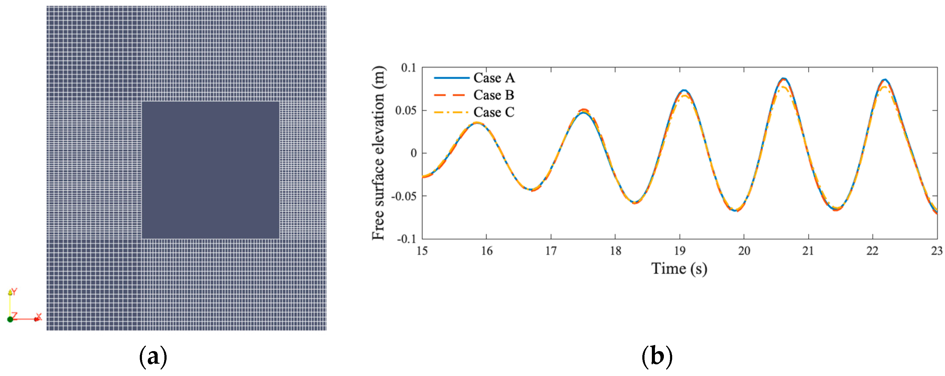
3.3. Computational Mesh

The computational meshes were constructed using OpenFOAM^®’s blockMesh utility. The meshes, featuring a rectangular cross-section around the floating pontoon, are depicted in Figure 3. Areas around the floating pontoon and near the free surface were refined with a refinement factor of 2. To ensure accuracy, a mesh convergence test was performed by comparing three test cases with different mesh sizes, as listed in

Table 2. Mesh refinement details for convergence testing. Here, L represents the wavelength, H is the wave height, and the x-axis and y-axis correspond to Figure 3. Computational time is measured with an end time of 25 s.

Test Cases	Mesh Size in x-Axis	Mesh Size in y-Axis	Computational Time Using a Single Core (Unit: s)
Case A	L/360	H/20	349,225
Case B	L/290	H/16	104,778
Case C	L/180	H/10	42,957

.

Surface elevations of transmitted waves at the lee side of the breakwater system were measured by Wave Gauge 2, located 2.5 m downstream of pontoon 2 (see Figure 1). Figure 3b presents a comparison of the time histories of free surface elevation at Wave Gauge 2 for all three mesh resolutions listed in Table 2, over the period from 15 s to 25 s, for a test case with an incident wave height H = 0.2 m and a wave period T = 1.58 s. The results indicate that cases a and b produced very similar outcomes, whereas case c consistently underestimated the crest elevation.

Based on the results of this convergence test, the mesh size of case b was selected for all simulations in this study.

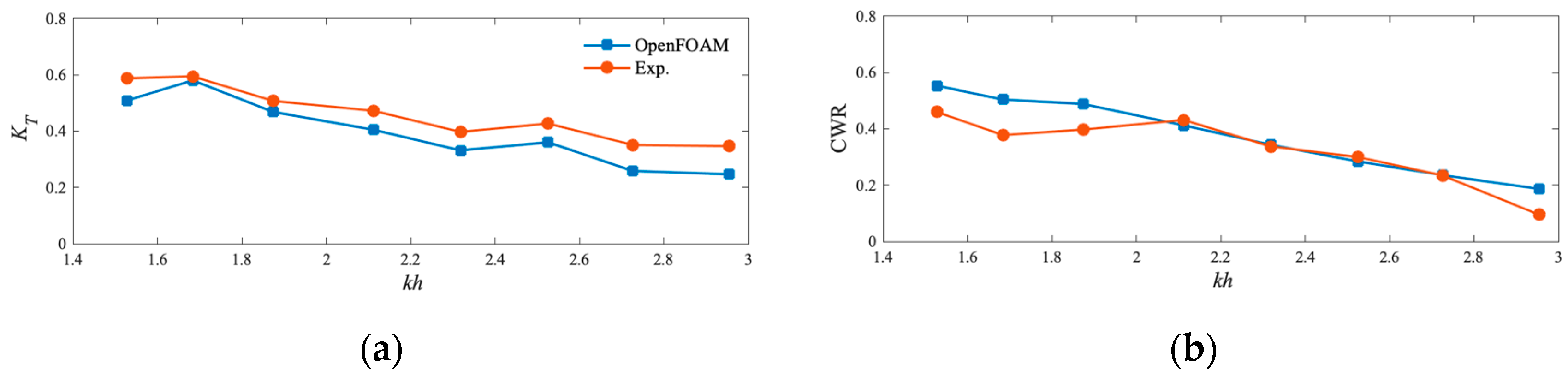
4. Model Validations

The numerical model was validated using experimental data collected from the wave tank at Dalian University of Technology [35]. The test conditions for the validation cases are detailed in

Table 3. Experimental setup conditions for the dual-pontoon system with B₁ = B₂ = 0.6 m, d₁ = d₂ =0.125 m, and D = 0.2 m. Here, T is the wave period, A is the wave amplitude, k is the wave number, h is the water depth, and kh represents the dimensionless wave number. The gravity of one pontoon is G = G₁ = G₂ = 1.5 N.

T (s)	1.17	1.22	1.27	1.33	1.4	1.5	1.6	1.7
A (m)	0.04	0.06	0.06	0.07	0.07	0.07	0.07	0.07
kh	2.954	2.726	2.526	2.318	2.112	1.874	1.684	1.528
FPTO/G	0.394	0.800	1.215	1.227	1.587	1.390	2.079	1.797

. A total of eight test cases with varying incident wave conditions were performed for validation. The PTO system’s damping forces, which maintain a constant magnitude under specific wave conditions and act in the direction opposite to the floating pontoons’ velocity, are also listed in Table 3.

The experimental and numerical results for two parameters, the transmission coefficient K_T and the capture width ratio (CWR), are compared in Figure 4, with each point representing the results for one test case. The numerical simulations using OpenFOAM^® accurately represent and predict both the variations and values of K_T when compared with experimental results. Furthermore, the CWR simulated by OpenFOAM^® closely matches the experimental results when $kh\ge 2.112$. However, for $1.528\le kh\le 1.874$, the numerical results slightly overestimate the CWR compared to the experimental data.

Figure 5 illustrates the energy balance in the test cases simulated by OpenFOAM^®. The wave energy P is proportional to H².

$${\displaystyle \frac{P_{reflected}}{P_{incident}}}={\displaystyle \frac{H_{reflected}^2}{H_{incident}^2}}=K_R^2,$$

(6)

$${\displaystyle \frac{P_{transmitted}}{P_{incident}}}={\displaystyle \frac{H_{transmitted}^2}{H_{incident}^2}}=K_T^2,$$

(7)

where $P_{incident}$, $P_{reflected}$, and $P_{transmitted}$ are the incident, reflected, and transmitted wave energies, respectively; H_incident, H_reflected, and H_transmitted denote the incident, reflected, and transmitted wave heights, respectively. Therefore, the proportion of energy comprising transmitted, reflected, and absorbed wave energy by WECs can be calculated as $K_T^2+K_R^2+\mathrm{C}\mathrm{W}\mathrm{R}$.

In an ideal scenario without energy dissipation, $K_T^2+K_R^2+\mathrm{C}\mathrm{W}\mathrm{R}$ should equal 1. However, vortex shedding around the floating pontoons, which can be simulated by OpenFOAM^®, induces energy dissipation. As a result, $K_T^2+K_R^2+\mathrm{C}\mathrm{W}\mathrm{R}$ in OpenFOAM^® simulations does not equal 1, as shown in Figure 5. The dissipation coefficient $C_d$ is calculated as ${1-(K}_T^2+K_R^2+\mathrm{C}\mathrm{W}\mathrm{R})$. When $1.528\le kh\le 1.874$, C_d is very low, indicating that the OpenFOAM^® simulations are close to idealised conditions. In physical experiments, friction loss and the effects of the wave flume’s sidewalls cannot be avoided, leading to lower CWR values compared to OpenFOAM^® results. These effects are expected to be larger in longer wave conditions, as noted in [35]. This discrepancy may explain the differences observed in Figure 4b only when kh is small ($1.528\le kh\le 1.874$). As kh increases, C_d generally increases, meaning that energy dissipation due to vortex shedding becomes the dominant factor for energy loss. Therefore, the difference between the numerical and experimental results becomes relatively smaller overall.

In summary, the numerical model demonstrates good performance in simulating the wave–structure interactions of the pile-restrained WEC-type dual-floating breakwater system. The model is stable and accurate enough to predict and evaluate the performance of this WEC-B system effectively.

5. Numerical Results and Discussion

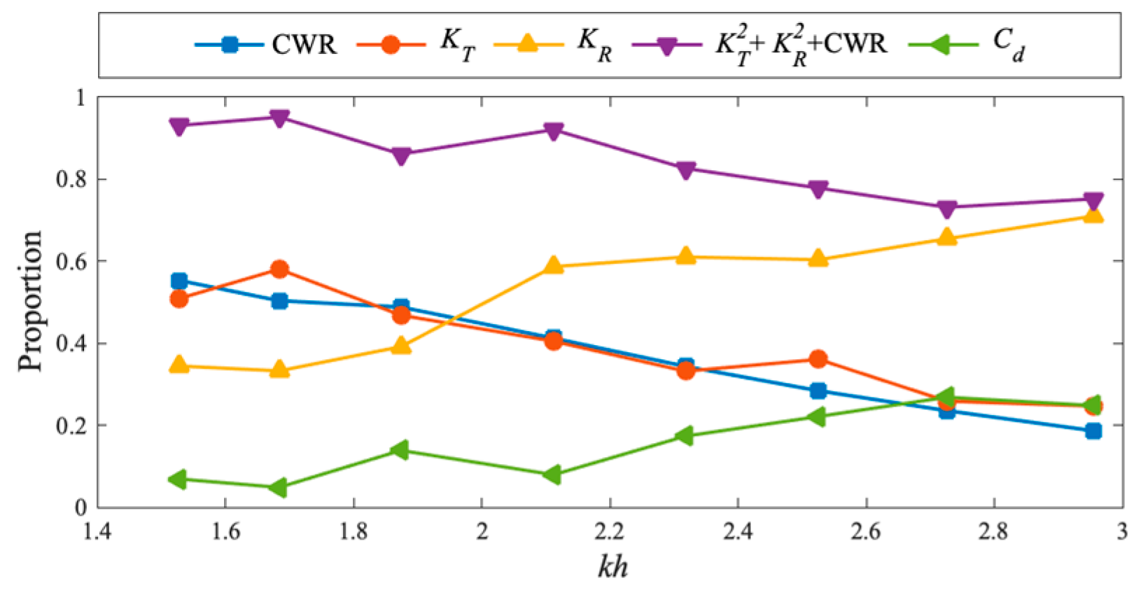
5.1. Wave Transmission Coefficient K_T and Capture Width Ratio CWR

The variations of K_T and the CWR as functions of the dimensionless wave number (kh) for the test groups summarised in Table 1 are presented in Figure 6 and Figure 7.

The values of K_T, in all cases, decrease with increasing kh. In each K_T vs. kh diagram, the dashed line represents a constant value of K_T = 0.5, considered an acceptable efficiency for wave attenuation [36]. Points below this dashed line indicate a satisfactory breakwater performance. These variations show that the floating breakwater system performs well in reducing the transmitted wave height in the high-frequency region (kh > 2). However, in the low-frequency region (kh < 2), K_T values are higher, demonstrating that the floating breakwater is less effective at attenuating long-period waves. Additionally, the K_T vs. kh curves (Figure 6 and Figure 7) reveal a general trend of a decreasing K_T with an increasing PTO damping coefficient. However, this decrease is not significant, likely because the damping forces from the PTO system are much smaller than the self-weight of each floating pontoon. Consequently, changes in the damping coefficient λ_PTO have only a minor impact on K_T.

Figure 6 and Figure 7 also show that the CWR increases with increasing kh when kh is small. After reaching a peak, the CWR starts to decrease as kh continues to increase. The dashed line at CWR = 0.2 in each CWR vs. kh plot indicates an acceptable efficiency for energy extraction [37], with points above this line signifying a satisfactory WEC performance. Each figure shows a specific range of kh where an acceptable WEC performance is achieved. Notably, the results for case e exhibit a slight oscillation in the CWR curves in the high-frequency regions. This phenomenon may be due to strong reflected waves at the front floating pontoon, leading to Bragg resonance. Bragg resonance occurs when the wavelength of incoming waves is approximately twice the spacing between structures, leading to constructive interference and strong wave reflections [38]. This phenomenon can significantly affect the hydrodynamic performance of the WEC-B system. In these simulations, Bragg resonance is observed when the gap width between the pontoons is 1.0 m. The strong reflected waves at the front floating pontoon interact with the incoming waves, creating a condition where the wave energy is amplified due to constructive interference. This interaction significantly alters the heave displacement of the floating pontoons across different frequencies. Previous studies [39,40] have highlighted the influence of Bragg resonance on arrays of multiple floating buoys, demonstrating that such resonance can lead to oscillations in the hydrodynamic responses. In this case, when the gap width is 1.0 m, the condition for Bragg resonance is met, causing the reflected waves from the upstream pontoon to interact with the incoming waves more strongly. This interaction increases the amplitude of the wave motion and, consequently, the heave displacement of the pontoons. As a result, case e exhibits slight oscillations in the CWR curves in the high-frequency regions, indicating the impact of Bragg resonance on the system’s performance.

PTO damping (λ_PTO) also affects CWR, and Figure 8 suggests that an optimal damping coefficient exists, varying with wave conditions.

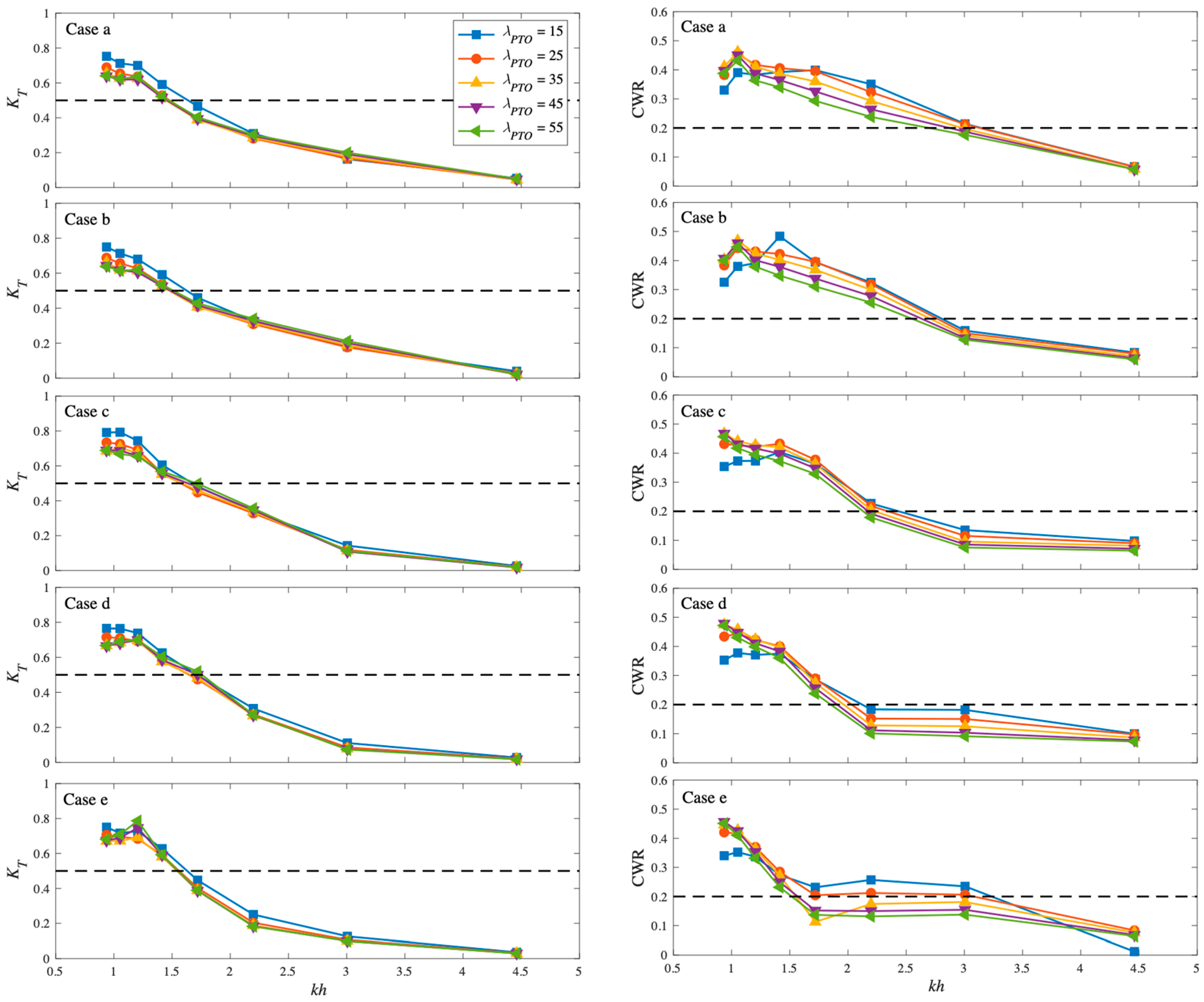
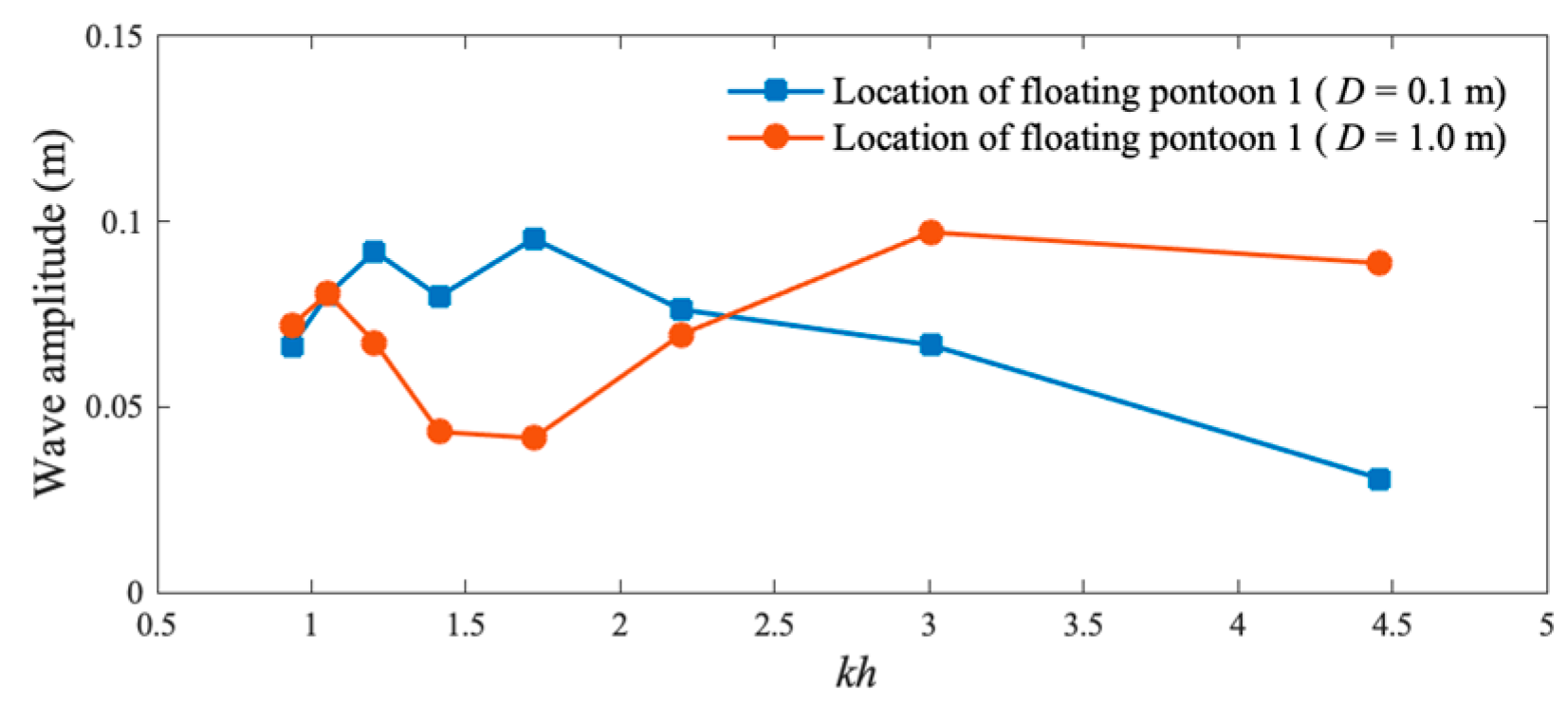
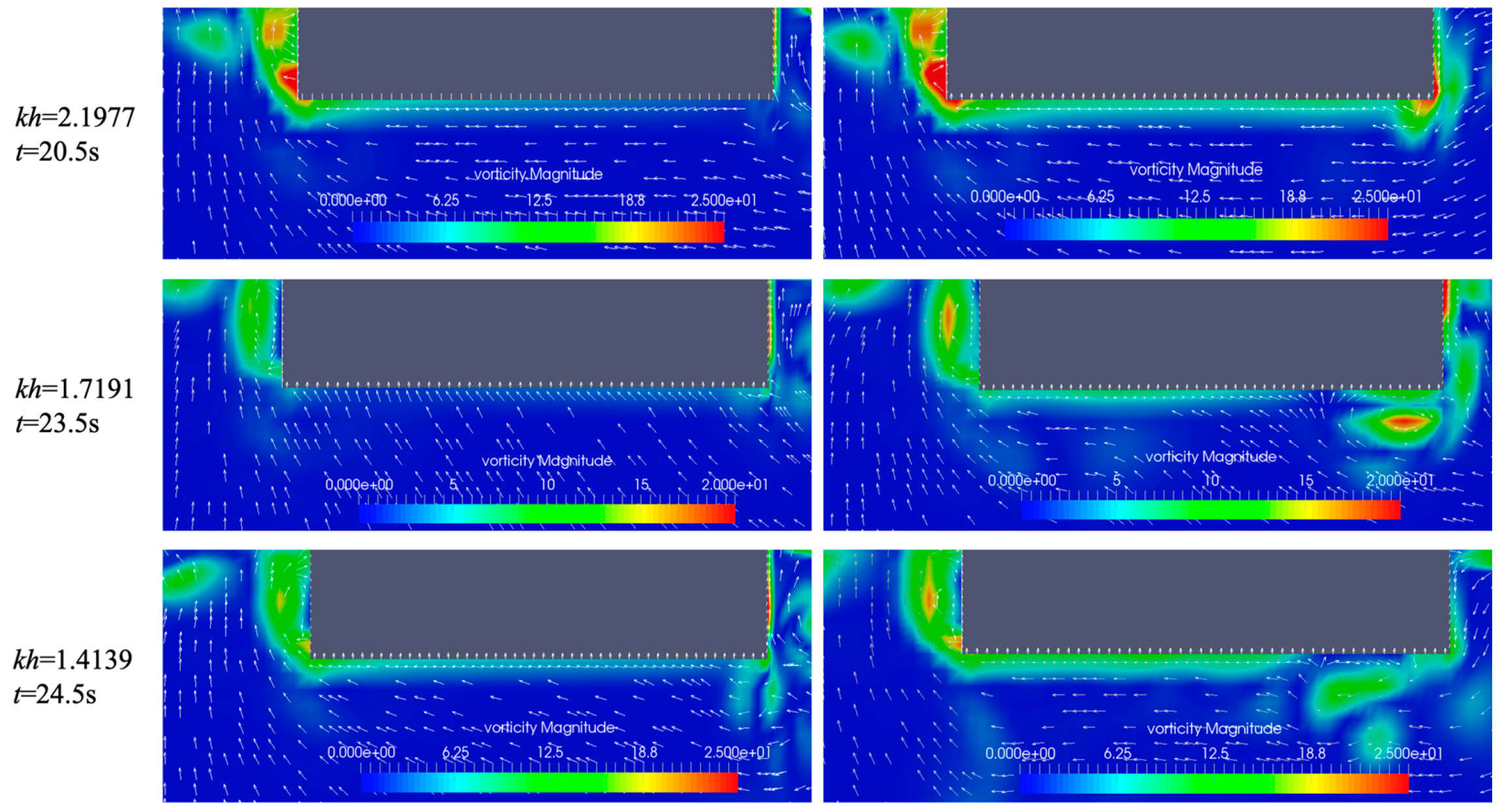
5.2. Effect of Gap Width

Figure 9 illustrates the influence of gap width D on K_T and the CWR. There is no obvious systematic influence of D on K_T. However, the CWR decreases with increasing gap width for kh > 1. As the gap width increases, the range of kh where the CWR remains acceptable (CWR > 0.2) diminishes. This indicates that smaller gap widths (ranging from 0.1 m to 1.0 m in the investigated scale) enhance the wave energy extraction performance of WEC-Bs.

To explore these observations further, Figure 10 presents the CWR and heave displacement of each individual pontoon separately. It is evident that the significant differences in the CWR are associated with the front floating pontoon (pontoon 1). Larger heave displacements correspond to more work being done by the PTO system, resulting in greater energy conversion by the WEC and higher CWR values. Thus, the larger CWR is primarily due to the greater heave displacement of pontoon 1 when the gap width D is 0.1 m. The reflected wave component and the vortex field are identified as the two primary factors affecting the heave displacements.

To analyse the reflected waves from pontoon 2, a series of tests were conducted with only pontoon 2 included and a wave gauge placed at the location of pontoon 1. Figure 11 shows the wave amplitude at the location of pontoon 1 for gap widths D = 0.1 m and D = 1.0 m. This wave amplitude at pontoon 1 is the superposition of the incident and reflected wave components. It is observed that the wave amplitude for D = 0.1 m differs from that for D = 1.0 m due to phase differences between the incident and reflected waves. For kh < 2.2, the wave amplitude with D = 0.1 m is larger than that with D = 1.0 m, whereas for kh > 2.2, the wave amplitude with D = 0.1 m is smaller. The relationship between wave amplitude and kh typically matches the trend of heave displacement. This indicates that the wave amplitude, influenced by the reflected wave component, is a significant factor affecting the heave displacement of pontoon 1. Additionally, the marked increase in wave amplitude with D = 1.0 m for kh > 2 in case e (Figure 6) demonstrates that the reflected wave component can also cause the second peak in the CWR vs. kh curves when D = 1.0 m.

In addition to the reflected waves, the vorticity field is another factor influencing the heave displacement. When the floating pontoon moves in a viscous fluid, vortex formation and low-pressure areas occur due to boundary layer separation, with the lowest pressure at the vortex core. This results in the fluid velocity opposing the direction of the floating pontoon, generating significant drag force when vorticity is high. This drag force can resist the heave motion of the pontoon. Figure 12 shows snapshots of the vorticity field around pontoon 1 when the wave crest reaches the pontoon for various wave conditions. Three wave conditions for two test groups, D = 0.1 m and D = 1.0 m, are presented. These snapshots indicate that vortices primarily concentrate at the sharp corners of the pontoon’s cross-section. The vortex at the lower left corner changes slightly with varying gap widths and wave amplitudes. However, notable changes occur with the vortex at the right corner in the gap between the pontoons. This suggests that different gap widths influence the vortex field around pontoon 1, with smaller gap widths reducing vorticity, allowing for greater heave displacement.

In summary, for multi-body systems, varying gap widths affect the rear pontoon’s influence on the wave amplitude at the front pontoon’s location and the vortex field around the pontoon. These two factors directly impact the heave motion of the pontoon, which determines the efficiency of wave energy extraction. For the test cases considered in this study, smaller gap widths enhance the efficiency of wave energy extraction.

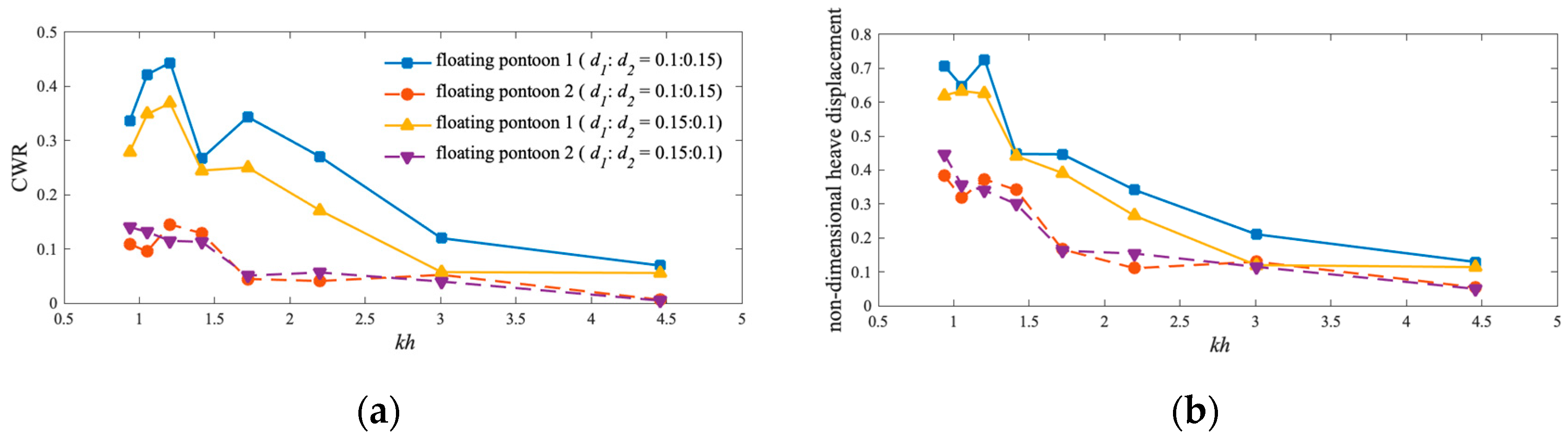
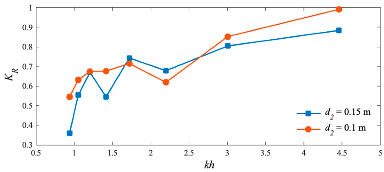
5.3. Effect of Structure Draft Ratio

Figure 13 shows that the structure draft D has only a minor influence on K_T, but significantly affects the CWR. Generally, a smaller d₁ leads to an increase in the CWR and a larger range of kh for acceptable CWR values above 0.2.

A detailed analysis of the draft’s influence on the CWR distribution for each floating pontoon is presented in Figure 14. It is evident that the CWR and heave displacement of floating pontoon 2 with d₁:d₂ = 0.1:0.15 are almost identical to those with d₁:d₂ = 0.15:1. The differences in CWR values are primarily attributed to the CWR of floating pontoon 1. As discussed in Section 5.2, the larger heave displacement of floating pontoon 1 with d₁ = 0.1 contributes to the increased CWR.

To further investigate the differences in heave displacement, the reflected waves and the vorticity field are examined. Figure 15 shows the reflection coefficients for different wave conditions with only floating pontoon 2 in the wave tank for two different structure drafts. It is observed that the draft has only a minor effect on reflected waves, indicating that reflected waves are unlikely to influence heave displacement due to changes in the structure draft. Figure 16 illustrates that vorticity around floating pontoon 1 decreases with decreasing draft, and the velocity field shows that deeper drafts result in a stronger vortex field that resists the pontoon’s motion. Thus, this is likely the reason for the increased heave motion of floating pontoon 1.

In summary, the observed influence of draft on the CWR for floating pontoon 1 is primarily due to changes in the vorticity field around the pontoon. The numerical results suggest that decreasing d₁:d₂ can enhance the wave energy extraction performance of the WEC-B system.

5.4. Effect of Structure Breadth Ratio

As shown in Figure 17, the structure breadth does not systematically influence K_T or CWR across the range of kh investigated. However, a reduction in B₁ slightly increases the range of kh for which the CWR is acceptable (CWR > 0.2).

Figure 18 presents the variation of the CWR and heave displacement with kh for the two floating pontoons individually. It is observed that the CWR and heave displacement of floating pontoon 1 with B₁ = 0.4 m are smaller than those with B₁ = 0.6 m. Conversely, the CWR and heave displacement of floating pontoon 2 with B₂ = 0.8 m are larger than those with B₂ = 0.6 m. These differences in CWR distributions contribute to the overall variations in the CWR curves of the holistic WEC-B system, shown in Figure 17.

Figure 19 shows that the structure breadth has a minor influence on the reflection coefficient K_R from floating pontoon 2. However, decreasing the structure breadth increases K_T for floating pontoon 1. This indicates that higher wave transmission past pontoon 1 will increase the heave motion of floating pontoon 2 as the structure breadth decreases. Nevertheless, the reflected waves from floating pontoon 2 do not significantly influence the heave motion of floating pontoon 1. The larger heave motion of floating pontoon 1 with B₁ = 0.6 m may be attributed to the smaller vorticity around pontoon 1, as shown in Figure 20. The vorticity in the gap decreases when B₁:B₂ = 0.6:0.6, likely due to different relative motions between the two pontoons with varying structure breadths. Thus, the different relative motions of pontoon 1 are primarily influenced by vorticity, while the relative motions of pontoon 2 are mainly affected by transmitted waves.

In summary, the differences in CWR for various structure breadths are primarily due to K_T from pontoon 1 and the vortex field. It was found that a smaller B₁:B₂ ratio can slightly increase the range of kh for an acceptable CWR in this WEC-B system.

5.5. Bandwidth of Effective Frequency

Based on the acceptable K_T [36] and CWR [37] values discussed in Section 5.1, the bandwidth of effective frequency (B_w) can be determined where both criteria are met. This bandwidth of effective frequency can be used to evaluate the overall performance of the WEC-B system, considering both wave attenuation and wave energy extraction. A WEC-B system with a wider effective frequency bandwidth can meet both criteria under a wider variety of wave conditions, making it a better-performing, multi-functional hybrid system.

Three diagrams in Figure 21 illustrate the variations of B_w against the damping coefficient for different gap widths, drafts, and structure breadths, respectively. Generally, a system with a smaller D, smaller d₁:d₂, and smaller B₁:B₂ increases the effective frequency bandwidth (B_w), thereby enhancing the overall performance of the WEC-B system. However, there are two outliers in the B_w vs. λ_PTO curves for D =1.0m. These outliers are caused by the second peak in the CWR vs. kh curves shown in case e in Figure 6. When λ_PTO = 15 kg/s and 25 kg/s, the CWR vs. kh curve rises above 0.2, which increases B_w at these two points.

6. Conclusions

In this paper, a numerical model based on OpenFOAM^® is used to investigate the performance of the WEC-B system. The study examines multiple parameters and analyses the vortex field and wave propagation to understand how different parameters affect performance. The key findings are:

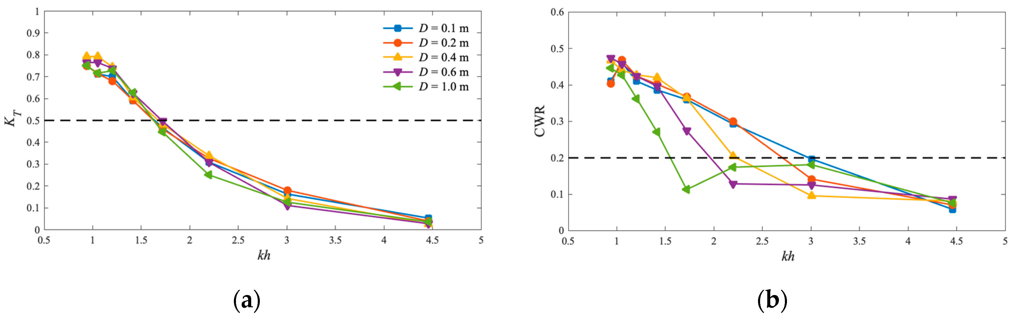
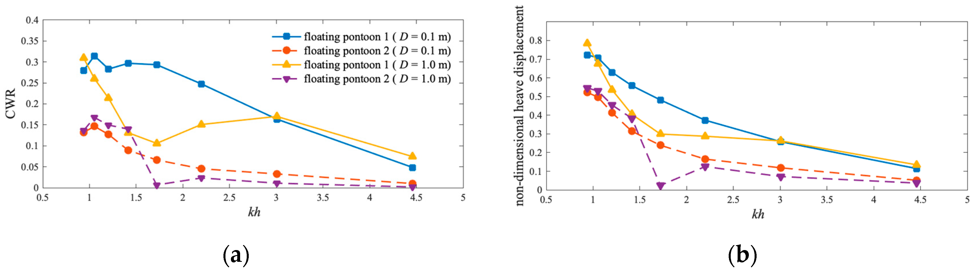
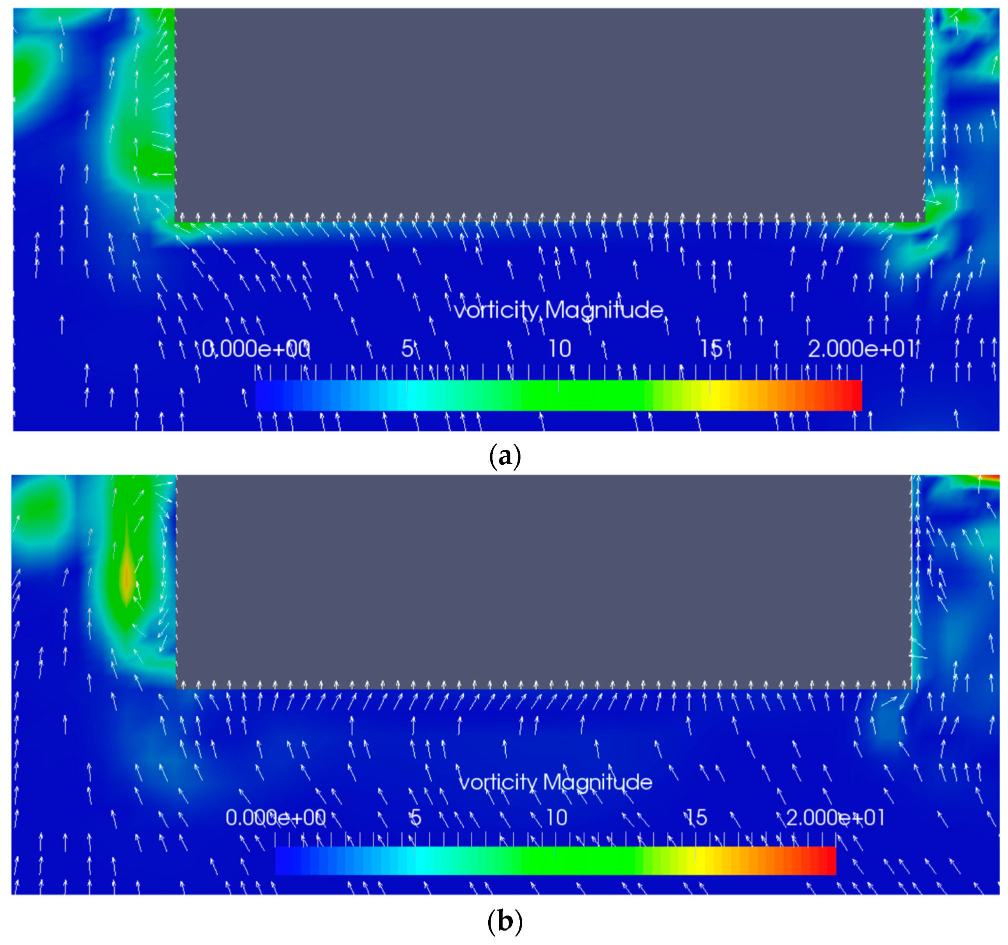
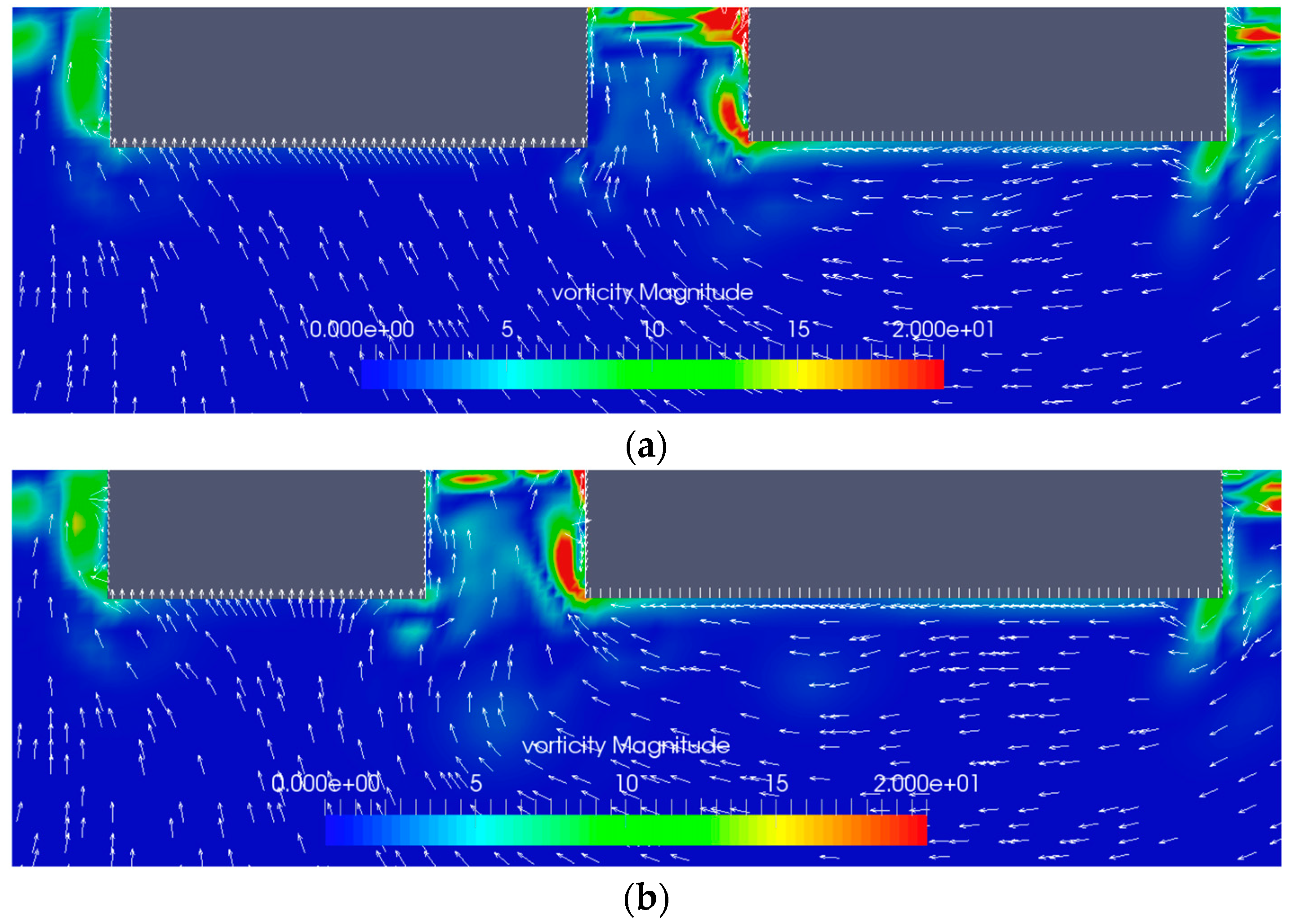
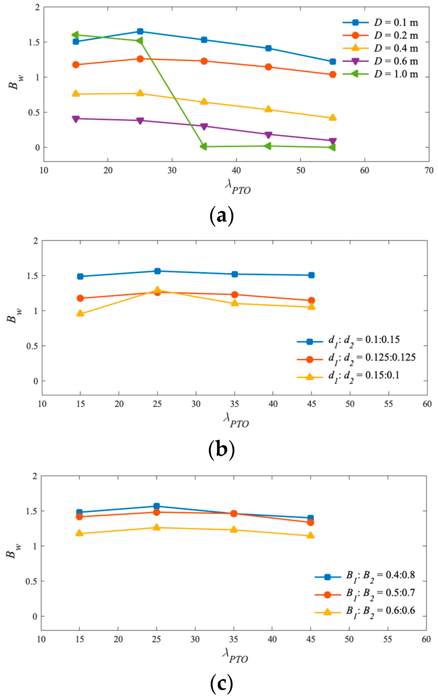
• Gap width impacts the vorticity field around the floating pontoon; a smaller gap width reduces vortices, increasing heave displacement and improving functional performance. A smaller gap width (ranging from 0.1 m to 1.0 m) can improve wave energy extraction efficiency.
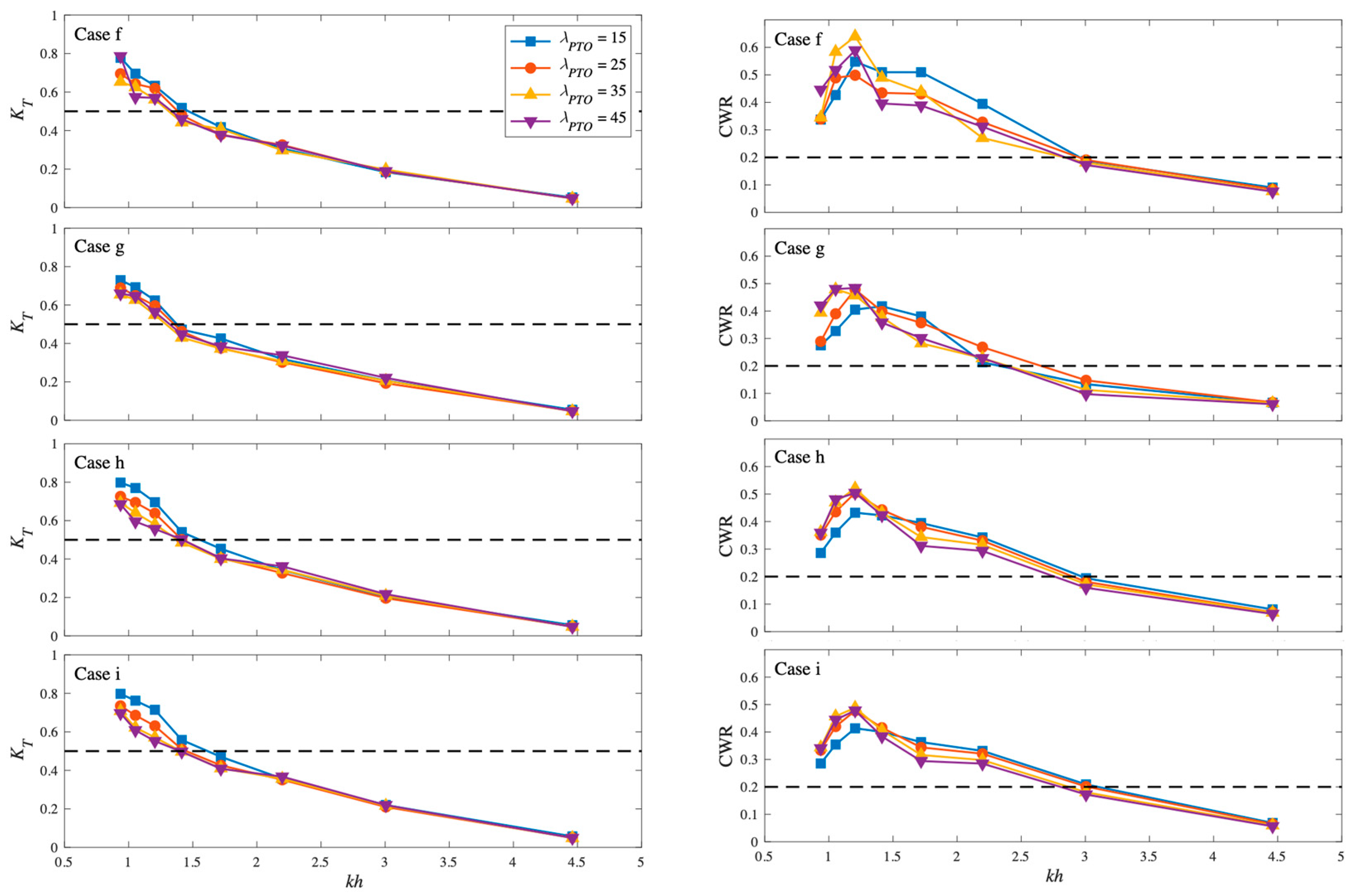
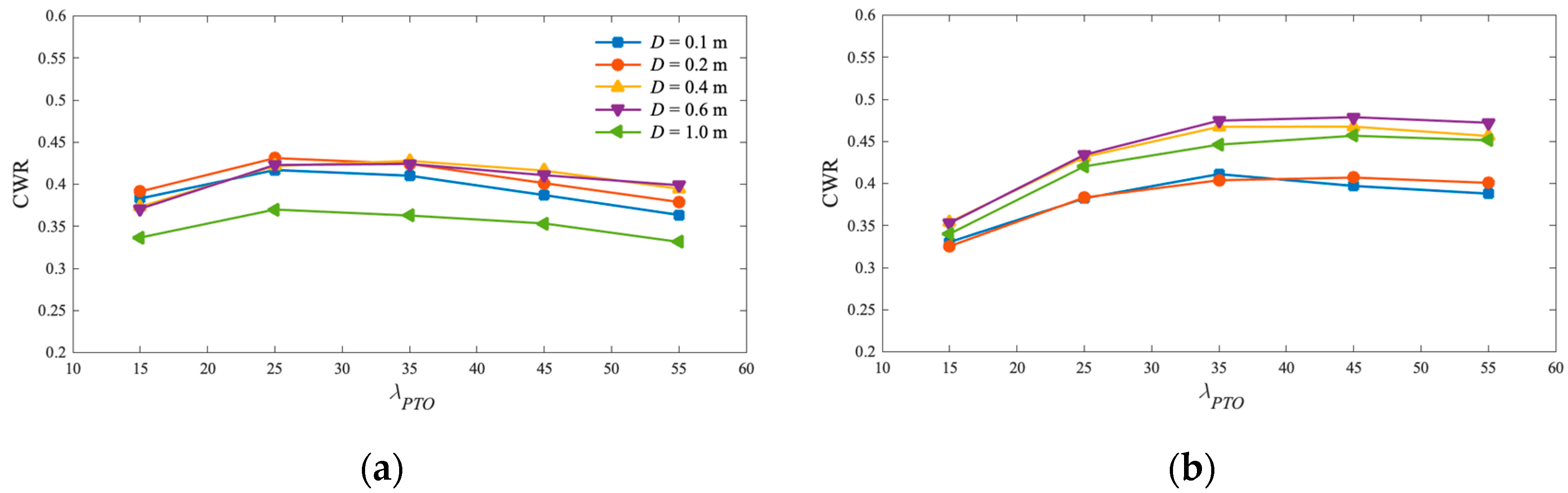
• Draft affects the vorticity field; a smaller draft reduces vortices and enhances performance. In this study, a smaller d₁:d₂ ratio improves performance. For instance, when d₁:d₂ = 0.1:0.15, the CWR can reach the best efficiency of 64%.
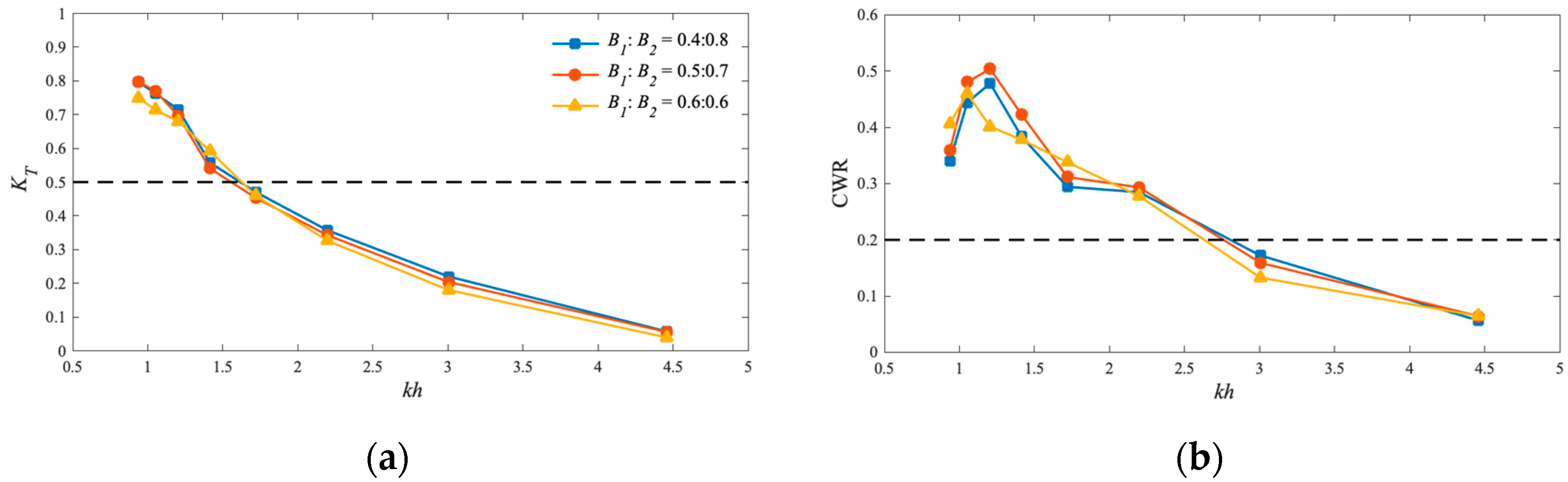
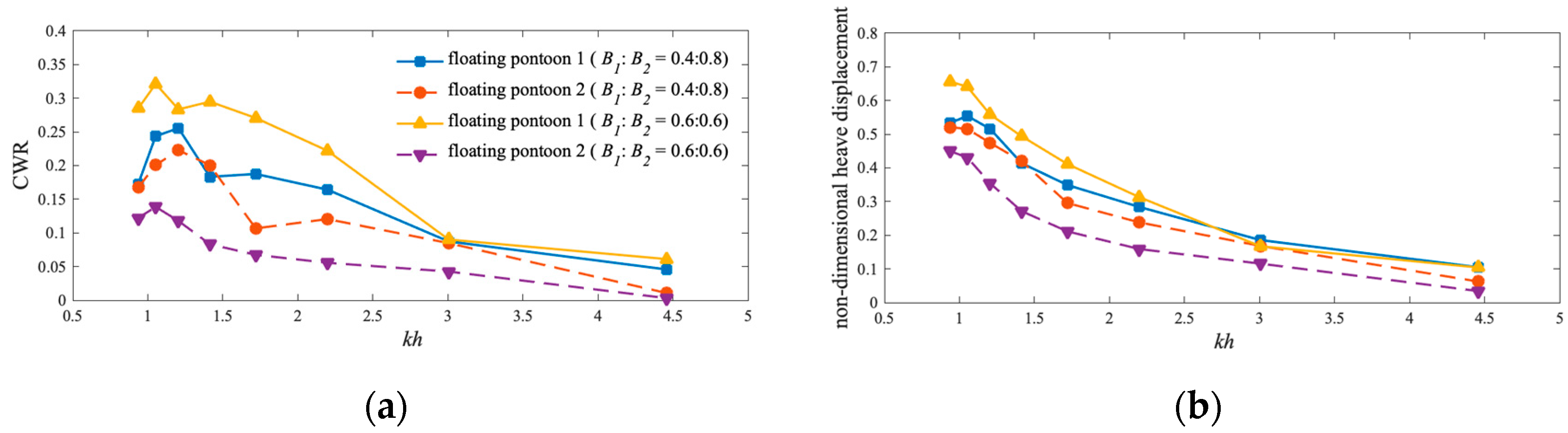
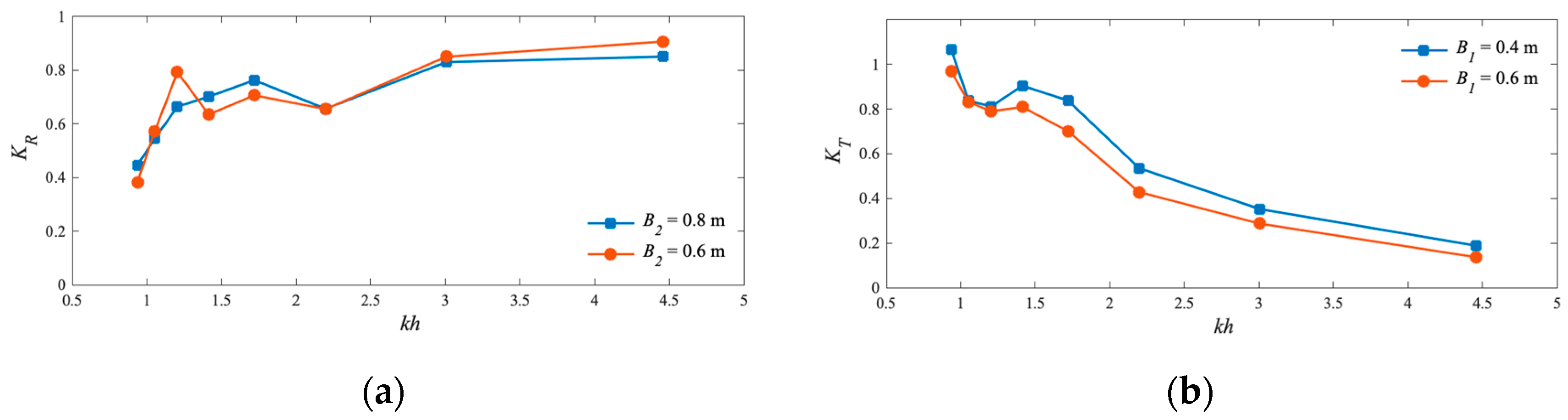
• Structure breadth influences wave reflection and transmission; a smaller B₁:B₂ ratio, when B₁:B₂ = 0.4:0.8, leads to better performance.
• Sharp changes in the high-frequency region of CWR vs. kh curves are due to Bragg reflection, which affects the effective frequency bandwidth. This factor should be considered in the design of integrated WEC and dual floating breakwaters.

This research includes the full consideration of flow viscosity using OpenFOAM^®, optimisation of the WEC-B system’s relative dimensions and layout, and the novel discussion of the effective frequency bandwidth to evaluate the overall functional performance. These findings suggest that further development of the WEC-B system is warranted.

This research highlights two main directions for enhancing the performance of WEC-B systems. First, increasing the utilisation of reflected waves by modifying the floating structure can improve efficiency. Second, improving the motion response of the floating pontoons by reducing vortices around the structures can enhance energy extraction. These practical applications can significantly contribute to the development of cost-effective and efficient WEC-B systems for sustainable energy generation.

References

1. Vicinanza, D.; Contestabile, P.; Nørgaard, J.Q.H.; Andersen, T.L. Innovative rubble mound breakwaters for overtopping wave energy conversion. Coast. Eng. 2014, 88, 154–170. [Google Scholar] [CrossRef]
2. Brooke, J. Wave Energy Conversion; Elsevier: Amsterdam, The Netherlands, 2003. [Google Scholar]
3. Falnes, J. Ocean Waves and Oscillating Systems: Linear Interactions Including Wave-Energy Extraction Johannes. Dev. Sedimentol. 1993, 52, 11–28. [Google Scholar] [CrossRef]
4. Martinelli, L. Wave Energy Converters under mild wave climates. OCEANS’11 MTS/IEEE KONA, Waikoloa, HI, USA, 19–22 September 2011; IEEE: Washington, DC, USA, 2017; pp. 1–8. [Google Scholar] [CrossRef]
5. Güney, M.S.; Kaygusuz, K. Hydrokinetic energy conversion systems: A technology status review, Renew. Sustain. Energy Rev. 2010, 14, 2996–3004. [Google Scholar] [CrossRef]
6. Waveplam Project. 2010. Available online: www.waveplam.eu (accessed on 8 August 2024).
7. Takahashi, S. Hydrodynamic Characteristics of Wave-power-extracting Caisson Breakwater. Coast. Eng. 1989, 2489–2503. [Google Scholar] [CrossRef]
8. Takahashi, S.; Nakada, H.; Ohneda, H.; Shikamori, M. Wave Power Conversion by a Prototype Wave Power Extracting Caisson in Sakata Port. In Proceedings of the 23rd International Conference on Coastal Engineering, Venice, Italy, 7–9 September 2015; pp. 3440–3453. [Google Scholar] [CrossRef]
9. He, F.; Huang, Z.; Law, A.W.-K. Hydrodynamic performance of a rectangular floating breakwater with and without pneumatic chambers: An experimental study. Ocean Eng. 2012, 51, 16–27. [Google Scholar] [CrossRef]
10. Michailides, C.; Angelides, D.C. Modeling of energy extraction and behavior of a Flexible Floating Breakwater. Appl. Ocean Res. 2012, 35, 77–94. [Google Scholar] [CrossRef]
11. Zanuttigh, B.; Martinelli, L.; Castagnetti, M.; Ruol, P.; Kofoed, J.P.; Frigaard, P. Integration of wave energy converters into coastal protection schemes. Icoe 2010, 2010, 1–7. [Google Scholar]
12. Zanuttigh, B.; Angelelli, E. Experimental investigation of floating wave energy converters for coastal protection purpose. Coast. Eng. 2013, 80, 148–159. [Google Scholar] [CrossRef]
13. Ning, D.; Zhao, X.; Göteman, M.; Kang, H. Hydrodynamic performance of a pile-restrained WEC-type floating breakwater: An experimental study. Renew. Energy 2016, 95, 531–541. [Google Scholar] [CrossRef]
14. Ning, D.Z.; Zhao, X.L.; Zhao, M.; Hann, M.; Kang, H.G. Analytical investigation of hydrodynamic performance of a dual pontoon WEC-type breakwater. Appl. Ocean Res. 2017, 65, 102–111. [Google Scholar] [CrossRef]
15. Reabroy, R.; Zheng, X.; Zhang, L.; Zang, J.; Yuan, Z.; Liu, M.; Sun, K.; Tiaple, Y. Hydrodynamic response and power efficiency analysis of heaving wave energy converter integrated with breakwater. Energy Convers. Manag. 2019, 195, 1174–1186. [Google Scholar] [CrossRef]
16. Zhang, H.; Zhou, B.; Vogel, C.; Willden, R.; Zang, J.; Geng, J. Hydrodynamic performance of a dual-floater hybrid system combining a floating breakwater and an oscillating-buoy type wave energy converter. Appl. Energy 2020, 259, 114212. [Google Scholar] [CrossRef]
17. Zhou, B.; Huang, X.; Lin, C.; Zhang, H.; Peng, J.; Nie, Z.; Jin, P. Experimental study of a WEC array-floating breakwater hybrid system in multiple-degree-of-freedom motion. Appl. Energy 2024, 371, 123694. [Google Scholar] [CrossRef]
18. Morgan, G.; Zang, J.; Greaves, D.; Heath, A.; Whitlow, C.; Young, J. Using the rasInterFoam CFD model for wave transformation and coastal modelling. In Proceedings of the 32nd Conference on Coastal Engineering, Shanghai, China, 30 June–5 July 2010. [Google Scholar]
19. Morgan, G.; Zang, J. Application of OpenFOAM to Coastal and Offshore Modelling. In Proceedings of the 26th Internation Workshop on Water Waves, Athens, Greece, 17–20 April 2011; pp. 3–6. [Google Scholar]
20. Jacobsen, N.G.; Fuhrman, D.R.; Fredsøe, J. A wave generation toolbox for the open-source CFD library: OpenFoams. Int. J. Numer. Methods Fluids 2012, 70, 1073–1088. [Google Scholar] [CrossRef]
21. Chen, L.F.; Zang, J.; Hillis, A.J.; Morgan, G.C.J.; Plummer, A.R. Numerical investigation of wave-structure interaction using OpenFOAM. Ocean Eng. 2014, 88, 91–109. [Google Scholar] [CrossRef]
22. Chen, L.F.; Zang, J.; Hillis, A.J.; Plummer, A.R. Numerical study of roll motion of a 2-D floating structure in viscous flow. J. Hydrodyn. 2016, 28, 544–563. [Google Scholar] [CrossRef]
23. Ferziger, J.H.; Peric, M. Computational Methods for Fluid Dynamics; Springer: Berlin/Heidelberg, Germany, 2012. [Google Scholar]
24. Issa, R.I. Solution of the Implicitly Discretised Fluid Flow Equations by Operator-Spliting. J. Comput. Phys. 1984, 62, 40–65. [Google Scholar] [CrossRef]
25. Courant, R.; Friedrichs, K.; Lewy, H. On the Partial Difference Equations of Mathematical Physics. IBM J. Res. Dev. 1967, 11, 215–234. [Google Scholar] [CrossRef]
26. Greenshields, C.J. OpenFOAM Guide. 2014. Available online: https://openfoamwiki.net/index.php/OpenFOAM_guide (accessed on 8 August 2024).
27. Hirt, C.W.; Nichols, B.D. Volume of fluid (VOF) method for the dynamics of free boundaries. J. Comput. Phys. 1981, 39, 201–225. [Google Scholar] [CrossRef]
28. Mayer, S.; Garapon, A.; Sørensen, L.S. A fractional step method for unsteady free-surface flow with applications to non-linear wave dynamics. Int. J. Numer. Methods Fluids 1998, 28, 293–315. [Google Scholar] [CrossRef]
29. He, Z.; Gao, J.; Shi, H.; Zang, J.; Chen, H.; Liu, Q. Investigation on effects of vertical degree of freedom on gap resonance between two side-by-side boxes under wave actions. China Ocean. Eng. 2022, 36, 403–412. [Google Scholar] [CrossRef]
30. Gao, J.; He, Z.; Huang, X.; Liu, Q.; Zang, J.; Wang, G. Effects of free heave motion on wave resonance inside a narrow gap between two boxes under wave actions. Ocean Eng. 2021, 224, 108753. [Google Scholar] [CrossRef]
31. Gao, J.L.; Lyu, J.; Wang, J.H.; Zhang, J.; Liu, Q.; Zang, J.; Zou, T. Study on transient gap resonance with consideration of the motion of floating body. China Ocean Eng. 2022, 36, 994–1006. [Google Scholar] [CrossRef]
32. Gong, S.-K.; Gao, J.-L.; Mao, H.-F. Investigations on fluid resonance within a narrow gap formed by two fixed bodies with varying breadth ratios. China Ocean Eng. 2023, 37, 962–974. [Google Scholar] [CrossRef]
33. Gao, J.; Mi, C.; Song, Z.; Liu, Y. Transient gap resonance between two closely-spaced boxes triggered by nonlinear focused wave groups. Ocean Eng. 2024, 305, 117938. [Google Scholar] [CrossRef]
34. Gong, S.; Gao, J.; Song, Z.; Shi, H.; Liu, Y. Hydrodynamics of fluid resonance in a narrow gap between two boxes with different breadths. Ocean Eng. 2024, 311, 118986. [Google Scholar] [CrossRef]
35. Ning, D.; Zhao, X.; Zang, J.; Johanning, L. Analytical and experimental study on a WEC-type floating breakwater. In Proceedings of the 12th European Wave and Tidal Energy Conference, Cork, UK, 27 August–1 September 2017; pp. 4–9. [Google Scholar]
36. Koutandos, E.; Prinos, P.; Gironella, X. Floating breakwaters under regular and irregular wave forcing: Reflection and transmission characteristics. J. Hydraul. Res. 2005, 43, 174–188. [Google Scholar] [CrossRef]
37. Babarit, A.; Hals, J.; Muliawan, M.J.; Kurniawan, A.; Moan, T.; Krokstad, J. Numerical benchmarking study of a selection of wave energy converters. Renew. Energy 2012, 41, 44–63. [Google Scholar] [CrossRef]
38. Gao, J.; Hou, L.; Liu, Y.; Shi, H. Influences of Bragg reflection on harbor resonance triggered by irregular wave groups. Ocean Eng. 2024, 305, 117941. [Google Scholar] [CrossRef]
39. Ouyang, H.T.; Chen, K.H.; Tsai, C.-M. Investigation on Bragg reflection of surface water waves induced by a train of fixed floating pontoon breakwaters. Int. J. Nav. Archit. Ocean Eng. 2015, 7, 951–963. [Google Scholar] [CrossRef]
40. Garnaud, X.; Mei, C.C. Bragg scattering and wave-power extraction by an array of small buoys. Proc. R. Soc. A Math. Phys. Eng. Sci. 2010, 466, 79–106. [Google Scholar] [CrossRef]
Figure 1. The WEC-B system configuration.
Energies 17 04046 g001
Figure 2. Computational domain of the numerical wave tank (with L representing the wavelength).
Energies 17 04046 g002
Figure 3. (a) Mesh configuration around a single floating body. (b) Free surface elevation results from three mesh refinement tests. The x-axis direction in (a) aligns with wave propagation.
Energies 17 04046 g003
Figure 4. Comparative analysis of experimental and numerical (a) wave transmission coefficient (KT) and (b) capture width ratio (CWR) across different kh values, as specified in Table 3.
Energies 17 04046 g004
Figure 5. OpenFOAM® results depicting wave reflection coefficient (KR), wave transmission coefficient (KT), capture width ratio (CWR), proportion of energy without dissipation ( K T 2 + K R 2 + C W R ), and dissipation coefficient (Cd) as functions of kh.
Energies 17 04046 g005
Figure 6. KT and CWR as a function of dimensionless wave number, kh, for different PTO system damping coefficients (λPTO, unit: kg/s) from case a to case e.
Energies 17 04046 g006
Figure 7. KT and CWR as a function of dimensionless wave number, kh, for different PTO system damping coefficients (λPTO, unit: kg/s) from case f to case i.
Energies 17 04046 g007
Figure 8. CWR as a function of λPTO for different gap widths with fixed draft and breadth ratios (d1:d2 = 0.125:0.125 and B1:B2 = 0.6:0.6). (a) CWR at kh = 1.2047 and (b) CWR at kh = 0.9366.
Energies 17 04046 g008
Figure 9. (a) KT and (b) CWR as a function of kh for different gap widths, with λPTO=35 kg/s. (d1:d2 = 0.125:0.125 and B1:B2 = 0.6:0.6).
Energies 17 04046 g009
Figure 10. Analysis of (a) CWR and (b) non-dimensional heave displacement for each pontoon as functions of kh with gap widths D = 0.1 m and 1.0 m. Heave displacement is normalised using a wave height of 0.12 m.
Energies 17 04046 g010
Figure 11. Wave amplitude at the location of floating pontoon 1 for gap widths D = 0.1 m and 1.0 m as a function of kh, with only floating pontoon 2 present in the wave tank.
Energies 17 04046 g011
Figure 12. Vorticity magnitude (Unit: s−1) and velocity vectors around floating pontoon 1 for gap widths D = 0.1 m (left panel) and 1.0 m (right panel).
Energies 17 04046 g012
Figure 13. (a) KT and (b) CWR as a function of kh for different drafts, with λPTO = 45 kg/s. (D = 0.2 m and B1:B2 = 0.6:0.6).
Energies 17 04046 g013
Figure 14. Analysis of (a) CWR and (b) non-dimensional heave displacement for each pontoon as functions of kh with draft ratios d1:d2 = 0.1:0.15 and 0.15:0.1. Heave displacement is normalised using a wave height of 0.12 m.
Energies 17 04046 g014
Figure 15. Wave reflection coefficient (KR, the ratio of reflected wave height to incident wave height) as a function of kh with only floating pontoon 2 present in the wave tank, for d2 = 0.15 m and 0.1 m.
Energies 17 04046 g015
Figure 16. Vorticity magnitude (Unit: s−1) and velocity vectors around the floating pontoon 1 for draft ratios d1:d2 = (a) 0.1:0.15 and (b) 0.15:0.1. Snapshot taken at 23.5 s, with kh = 1.7191.
Energies 17 04046 g016
Figure 17. (a) KT and (b) CWR as a function of kh for different structural breadths, with λPTO = 45 kg/s. (D = 0.2 m and d1:d2 = 0.125:0.125).
Energies 17 04046 g017
Figure 18. (a) CWR and (b) non-dimensional heave displacement for each pontoon individually as a function of kh with structure breadth ratios B1:B2 = 0.4:0.8 and 0.6:0.6. Heave displacement is normalised using a wave height of 0.12 m.
Energies 17 04046 g018
Figure 19. (a) Wave reflection coefficient (KR) with only floating pontoon 2 present in the wave tank, for B2 = 0.8 m and 0.6 m, and (b) wave transmission coefficient (KT) with only floating pontoon 1 present in the wave tank, for B1 = 0.4m and 0.6m, as functions of kh.
Energies 17 04046 g019
Figure 20. Vorticity magnitude (Unit: s−1) and velocity vectors around two floating pontoons for structure breadth ratios B1:B2 = (a) 0.4:0.8 and (b) 0.6:0.6. Snapshot taken at 23.5 s, with kh = 1.7191.
Energies 17 04046 g020
Figure 21. Bandwidth of effective frequency (Bw) as a function of damping coefficient (λPTO) with varying (a) gap widths, (b) drafts, and (c) structure breaths.
Energies 17 04046 g021