Abstract
The paper presents the application of a new bio-inspired metaheuristic optimization algorithm. The popularity and usability of different swarm-based metaheuristic algorithms are undeniable. The majority of known algorithms mimic the hunting behavior of animals. However, the current approach does not satisfy the full bio-diversity inspiration among different organisms. Thus, the Birch-inspired Optimization Algorithm (BiOA) is proposed as a powerful and efficient tool based on the pioneering behavior of one of the most common tree species. Birch trees are known for their superiority over other species in overgrowing and spreading across unrestricted terrains. The proposed two-step algorithm reproduces both the seed transport and plant development. A detailed description and the mathematical model of the algorithm are given. The discussion and examination of the influence of the parameters on efficiency are also provided in detail. In order to demonstrate the effectiveness of the proposed algorithm, its application to selecting the parameters of the control structure of a drive system with an elastic connection is shown. A structure with a PI controller and two additional feedbacks on the torque and speed difference between the drive motor and the working machine was selected. A system with rated and variable parameters is considered. The theoretical considerations and the simulation study were verified on a laboratory stand.
1. Introduction
1.1. Optimization Algorithms
The continuous development of new control structures, machines, systems, and electronics requires new tools for design, tuning, and maintenance. The best performance resulting in the highest profit is the paramount requirement, notwithstanding the research discipline. The popularity of artificial intelligence (AI) is unceasingly increasing, while the mathematical models for standard analysis are missing. Optimization tasks are widely used to find the parameters of the processes. To facilitate the calculation of the optimum, novel optimization algorithms are widely implemented. Thus, the increasing popularity of a certain group of optimization algorithms—metaheuristic algorithms inspired by observations of natural phenomena have become the most popular tools [1,2]. Their popularity in design applications is undeniable—the literature presents successful applications in different branches of economics [3], sciences [4], engineering [5], and medicine [6,7]. Because of its popularity, the group of nature-inspired algorithms is a research interest of scientists around the world. Not only are the new applications being investigated and examined, but known bio-inspired algorithms are also being improved and new optimizers are being developed. Numerous natural inspirations can be distinguished when reviewing bio-inspired algorithms (Figure 1)—e.g., inspirations from natural phenomena and physical laws [8,9,10], disease (virus and bacteria-based) spreading [11,12], animals, insects, plants [13,14], and even mushroom reproduction [15] have been published. Animal-inspired algorithms are the most common ones, as swarm intelligence for foraging can be easily mimicked—e.g., Artificial Bee Colony (ABC) [16], Ant Colony Optimization Algorithm (ACO) [17], Jellyfish Search Optimizer (JSO) [18], and Grey Wolf Optimizer (GWO) [19].
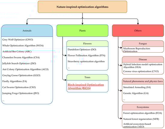
Figure 1.
Classification of nature-inspired optimization algorithms based on sources of inspiration.
The scheme of most metaheuristic optimization algorithms is similar and is based on the evolution or migration of specimens inside a population. The mechanism of reorganization of the population in the next iterations is based on the unique behavior of species. The review of the nature-inspired algorithms indicates an astounding niche among plant and tree inspirations. The reason for the absence of tree inspirations may be attributed to their immobility and poor adaptation to hunting. However, trees remain some of the tallest and oldest organisms in the world [20]. Trees have adapted to environmental conditions by developing specific propagation behaviors, seed shapes, and survival abilities. These were the inspiration for algorithms that mimic forestation [21]. To ensure the novelty of the proposed algorithm and enhance credibility, a comprehensive twofold review was conducted. The authors revised databases of notable journals and conferences based on keywords connected with trees and the most popular species—oak, maple, birch, pine, ash, and alder. To make the research even more reliable and to reduce the risk of oversight, the currently published review papers concerning nature-inspired optimization algorithms (NIOAs) were also examined. The authors of [22] provided a comprehensive study of 29 NIOAs, while [23] presented a couple of the algorithms and a standardization method for inspiration identification. The extended and updated version of NIOA’s “bible” [24] lists only a limited number of NIOAs, among which inspirations from trees are absent. A survey [25] draws a brief categorization map of NIOAs; however, it disregards inspirations with trees. Finally, [26] specifies 65 NIOAs developed in 2019–2021, which, in addition to the list of NIOAs reported before 2018 [27], accounts for a complete review foundation. Even though considerable efforts were devoted to the review, the authors were not able to find any algorithm based on a specific tree species. Thus, the Birch-inspired Optimization Algorithm (BiOA) presented in this paper is believed to be the first tree species-inspired metaheuristic optimizer. The considerations presented in the further parts of this paper provide an exceptional attribute of inspiration with the propagation of birch trees. The BiOA is not only the first tree-species-inspired NIOA, but it also introduces the possibility of parallel computation with subpopulations. This capability is especially desirable in modern multi-core workstations and should result in a substantial increase in optimization performance (and an evident reduction in computation time). The parallel version of the algorithm introduces the division of the search range into uniform subgroups.
1.2. Birch Tree—Inspiration
Silver birch is a deciduous tree. It is common in colder regions of Europe and Asia. Its range extends from the Pyrenees in the west, through the eastern part of Europe and Siberia to China and the Republic of Korea in the east. The southern range ends in Turkey and Iran. As an introduced species, it also occurs in North America. Depending on the climate, birch grows up to 30–40 m high and 80 cm in diameter. It has a characteristic white bark resulting from the presence of betulin (in the case of very young trees, the bark is brown). It is characterized by very rapid growth when young. Birch is a monoecious, deciduous species. Male inflorescences are formed at the end of summer, while female inflorescences are formed in spring. Male inflorescences produce significant amounts of pollen carried by the wind. After pollination, the female inflorescences transform into cones. Each husk has three nuts (seeds) with wings. The disintegration of cones begins at the end of summer and lasts until winter. Seeds can be carried long distances by the wind. The seeds usually germinate in the spring of the following year. Silver birch is a pioneer species, very quickly taking over exposed areas, for example, areas where agricultural production has ceased or areas after industrial production (e.g., on mine heaps). This is due to both the high ability to adapt to difficult environmental conditions and the method of reproduction. As shown in [28], birch occupies a dominant position among all tree species, considering the succession coefficient. It successfully covers areas with various environmental conditions, including polluted ones (in the research concerning central Europe). Similar conclusions are drawn from the research presented in [29]. In this case, the authors analyze tree successions in a mountainous region of the Alps with a short vegetation period. Here, too, birch was one of the first species to occupy the area. Other aspects regarding birch succession were presented in [30]. Birch is one of the most pioneering trees that colonize areas with various environmental conditions. This motivated the development of a metaheuristic algorithm based on the method of propagation of these trees. To the best of the authors’ knowledge, there is no such algorithm in the literature. Figure 2 shows photos of a birch growing alone and in a group. For an individual growing alone, you can notice a nicely developed tree crown with many branches, meaning a large number of seeds are produced. In the case of trees growing in a group, growth conditions are significantly more difficult. Trees compete with each other for access to nutrients and sunlight. As a consequence, each individual plant produces fewer seeds. These factors were taken into account in the developed algorithm.
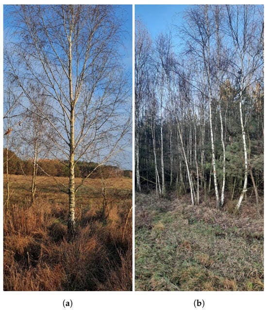
Figure 2.
Birch trees planted at the same time: a single specimen growing alone (a), a group of dwarf trees forming a thicket (b).
1.3. The Example of a BiOA Application—Electrical Drives
Electric motors are widely used in industry to drive production lines. They have a number of unquestionable advantages, such as their small size, resistance to environmental conditions, low level of generated interference, ease of shaping mechanical characteristics (in modern systems), and others. In order to increase the productivity of process lines, the aim is to shorten transition processes. This is achieved by forcing the drive state variables, electromagnetic torque and speed/position, more dynamically. Increased system dynamics, however, can reveal mechanical resonances associated with the mechanical connections found in drive systems. Torsional vibrations reduce the accuracy of the system’s velocity/position control and generate additional stresses in the couplings, which leads to a reduction in the reliability of the system (both by shortening the life and, in special cases, leading to sudden system failure) [31,32,33,34,35,36,37].
The problem of torsional vibration was the first to be described in high-power drives. Examples include rolling mills, conveyor belts, wind turbines, and machines in the textile or paper industries. In such systems, one can easily see the masses associated with the drive motor and the working machine connected by a long shaft (Figure 3) [31,32,33,34,35,36,38]. An analogous problem occurs in wind power plants. Wind energy is supplied to the generator through a mechanical shaft; in addition, a gearbox is used to allow speed changes [39]. With the increase in the dynamics of driving torque forcing, the problem of torsional vibration has become apparent in other systems: servo-drives, robots, or electromobility in the broadest sense [40,41,42,43,44]. A number of different methods have been proposed and presented in the literature to effectively suppress torsional vibration. In the general case, existing methods can be divided into two different groups: passive methods and active methods. The former includes the use of various types of filters. One of the most popular is the Notch filter placed in the speed controller. A relatively new approach is the use of resonant regulators. Passive methods allow the elimination of oscillatory components from the reference signal, thereby suppressing oscillations. However, they do not allow one to increase the dynamics of the drive system [45].
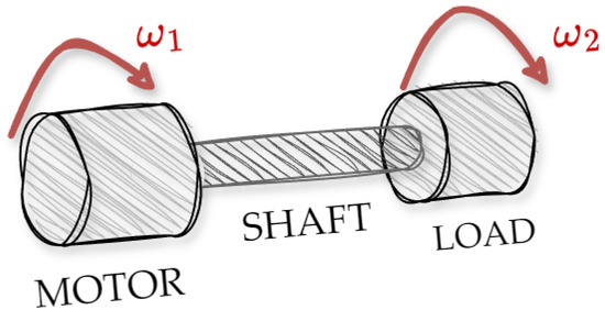
Figure 3.
Electric motor and load machine connected with flexible shaft–two-mass system.
In order to effectively suppress torsional vibration, it is necessary to use one of the active control methods. In the general case, they can be divided into several basic groups. The first of these include systems based on the classical PI controller [46]. However, their use is not effective in this case. Weakly damped oscillations can occur in the waveforms of the system’s variables. This is due to the impossibility of arbitrary arrangement of the poles of the closed control structure on the imaginary plane. In order to improve the efficiency of torsional damping, additional feedback from selected state variables is used. Particularly popular is the use of a signal from the torsional moment [47,48]. As shown in [46], there are nine possible individual feedbacks, which can be divided into three groups. Individual feedback can be introduced to both the torque and velocity node [46]. The addition of a single feedback provides effective torsional damping, but the build-up time depends on the parameters of the structure and cannot be determined by the designer. The use of two additional feedbacks in the system allows any arrangement of the poles of the closed system on the imaginary plane. Thus, it is possible to freely shape the characteristics of the system in the linear operating range (the main limiting factor is the maximum values of electromagnetic and torsional moments). Particularly popular is a system with additional coupling from torsional torque and speed difference. Another control structure is a system based on a state controller [49]. Since it has couplings from all state variables, it is possible to locate the poles of the closed system arbitrarily. The disadvantage of this approach is that it is not possible to limit the internal state variables of the system, the maximum value of the torsional torque transmitted by the shaft [49]. Another structure that provides effective torsional vibration damping is the FDC (Forced Dynamic Control) structure [50]. Unlike the previously mentioned ones, it allows both independent pole spacing and zero compensation of the closed system already at the design stage. This means that the system’s response to a change in the setpoint signal can be shaped, and, at the same time, the load torque can be compensated (theoretically ideal). The control system coefficients in the aforementioned systems, depend on the parameters of the object. Their change leads to a shift in the poles of the closed system from the designed location. Thus, this changes the designed characteristics of the system; in special cases, this can even lead to a loss of stability of the closed-loop control system. For applications with variable parameters, robust control should be used [51]. One solution is to use a classical control method with coefficients selected in such a way as to minimize the effect of parameter changes on the waveforms of the system variables. For this purpose, a specially selected objective function is defined, and, in turn, a suitable method of parameter selection is given. Such an approach is presented in this paper. The next popular method of controlling a system with variable parameters is the use of sliding control [52,53]. In this algorithm, two phases are distinguished, reaching and sliding. In the first, the system is sensitive to a change in parameters, while in the second, it is already resistant. The advantage of sliding control is that the structure can be made robust to changing parameters. Disadvantages include the form of the sliding function; in the case of a dual-mass system, it is necessary to have information about the output of the system and its first and second derivatives. Obtaining these quantities with high accuracy and low noise can be problematic in practical applications. Another disadvantage arises from the use of a discontinuous signum function. This results in chattering. It can be eliminated by replacing the discontinuous function with a linear approximation. However, this reduces the robustness of the structure to changing parameters. Another group of methods applied to a system with variable parameters is adaptive control [54,55,56,57]. In the general case, they can be divided into two groups: direct control and indirect control. In the latter, the characteristic element is the system for the identification of variable parameters. Based on the values of the identified parameters, the coefficients of the control system are tuned. The key element in this structure is the accuracy of parameter determination. The quality of operation of the entire structure depends on this. As an example, ref. [56] uses a Kalman filter to identify the variable parameter value of the working machine. The second group is direct control. On the basis of the setpoint and output from the object (possibly the control signal), the controller parameters are tuned. An example is the following work [57]. In recent years, there has been a growing interest in predictive control (especially Model Predictive Control) in electric drives [58,59]. This control involves defining a prediction window that calculates the future trajectories of an object and selecting the most optimal control sequence. The popularity of MPC is due to the undoubted advantages of this approach: the ability to shape the characteristics of the system over a wide range and to introduce constraints on the internal state variables of the object. Among the disadvantages of MPC is the very high computational complexity of the algorithm, which has been a limiting factor in its implementation over the years. Another disadvantage stems from the need for a good-quality model. Its inaccuracies cause erroneous trajectory calculations and thus reduce the quality of control. Advanced control methods require information about the vector of the state variables (and parameters) of the object. Since these are generally unavailable, various methods of estimating these variables are used. Among the most popular are systems based on the Luenberger observer. Kalman filters are recommended for high-noise systems. New approaches, such as the use of multi-observers, are also encountered in the literature. Estimation systems provide information about state variables for use in advanced control systems [60,61,62]. Despite the existence of various control methods, industrial applications are dominated by systems based on PI-type controllers. This is due to various factors. First, classical methods are very well known by engineers working in industry. Selecting the settings of these controllers, as well as checking, for example, stability, is no problem for operators. Secondly, the computing power of the controllers used in industry is also limited. The use of a relatively simple control algorithm makes it possible to devote more of the computing power to diagnostic and prognostic algorithms. A similar situation will arise when upgrading older industrial workstations. One seeks to minimize costs and use existing components. Thus, the development of a relatively simple immune control algorithm based on PI controllers is eagerly awaited by the industrial community.
The paper is focused on the proposition of the novel Birch-inspired Optimization Algorithm (BiOA) technique. It presents the inspiration, the mathematical background, and the test (including a comparison to other methods). Moreover, the real-life implementation is analyzed— the parameters used in the speed control structure of the nonlinear drive with an elastic connection are calculated. For the task, a laboratory experiment is presented. Based on the provided literature review and the current state of the art, the main contributions are as follows.
- The foundation of a new metaheuristic algorithm inspired by propagation and pioneering capability of birch trees—the Birch-inspired Optimization Algorithm (BiOA).
- Tests based on the benchmark functions prepared for the analyzed BiOA and other well-known algorithms—a comparison.
- The BiOA implementation for the optimization of the extended control structure of the two-mass system.
- Experimental validation of the results.
The organization of the paper is as follows. The first part Section 1.1 provides a review of nature-inspired optimization algorithms, draws a classification of metaheuristic algorithms based on the inspiration, and briefly discusses chosen applications. A general description of a birch tree (Betula pendula) is also included in the introduction of the paper Section 1.2. The introduction of the paper Section 1.3 also incorporates a brief description of modern electrical drives, control quality, and performance criteria defined for drives with an elastic connection. The next part, Section 2 provides a detailed characterization of the natural phenomena of birch propagation and stipulates the next steps of the developed BiOA. This section delivers a full mathematical description, including an explanation of the suggested values of the parameters used. The forthcoming section presents the results of the BiOA examination—the first part describes the effectiveness of the algorithm with chosen benchmark functions Section 3.1.1, Section 3.1.2 and Section 3.1.3. It also includes general performance assessment and comparison with other NIOAs Section 3.1.4. The second part of the results section gives the results of the real-life applications of the BiOA to a bin packing problem, Section 3.2.1 and the tuning of parameters of the speed controller of a two-mass system Section 3.2.2 to prove the desired applicability [63]. Both a simulation and an experiment are considered. The paper concludes with a discussion Section 4 and conclusion Section 5 sections where a brief summary is provided. These sections include a critical assessment of the gathered results and outline plans for further examination and potential improvements.
2. Mathematical Description of the Birch-Inspired Optimization Algorithm (BiOA)
The birch tree is known for its pioneer capability and the ability to sprout in various types of soil and ecosystems. These qualities make birch trees spread over unrestricted areas such as fields, dumpsites, wastelands, and burnt terrains [64,65].
Birch trees are known to create soil seed banks, which remain dormant and require moisture (which may be delivered randomly after storms) to germinate [66]. This behavior was modeled as the initial step of the proposed Birch-inspired Optimization Algorithm (BiOA). The first population is randomly generated similar to how seedlings sprout randomly. This can be described by Equation (1).
where d—indicator of solution dimension ( for D-dimensional task); —upper bound of optimization space; and —lower bound of optimization space. The random value is drawn with a continuous uniformly distributed random number generator. To improve the performance of BiOA in modern multi-core devices, the search range can be divided into smaller areas. In such a case, every subrange is exploited by a subpopulation. Every subpopulation is then calculated independently with a single core.
The BiOA consists of two steps that imitate seed propagation and subsequent sprout growth of the trees. The seed propagation mechanism focuses on the exploration of optimization space and the sprouting exploitation of the vicinity.
The propagation of birch trees occurs from July until the beginning of winter. The additional factor for pioneering areas in nearly all environments is the fact that birch is a monoecious tree. The pollen produced by male flowers is transferred to female flowers since early spring among even a single specimen [67]. The pollinated pistillate evolves into cones that can spread hundreds of seeds. It may be assumed that a single tree can produce 0.35 million up to 1.5 million seeds during an average year [68]. The production rate is the first parameter of the BiOA: , which is randomly drawn at the beginning of the optimization task. It should be noted that the given range for this parameter is strictly based on empirical observations of birch trees in middle-latitude, European forests. It was assumed that the more seeds produced, the higher the probability of long-distance flights.
The birch seed is equipped with bug-like wings (Figure 4); thus it is able to travel propelled by the wind. In comparison to dandelion seeds, these seeds are rather gliding and unceasingly falling (Figure 5). The traveled distance is a function of tree height, wind speed, and the type of environment [69]. Because of such behavior, this phenomenon can be modeled with a Levy flight function [70]; thus the step is defined by Equation (2). This relation is a common model of wind transfer, e.g., it is applied in the Flower Pollination Algorithm (FPA) for a global pollination case [71].
where —seed production rate; v—random value, ; u—random value, ; and is defined by formula (Equation (3)):
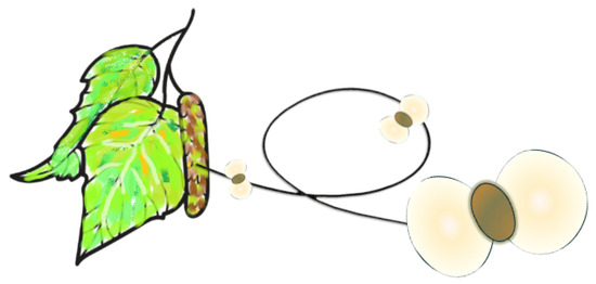
Figure 4.
Flight of birch seeds.
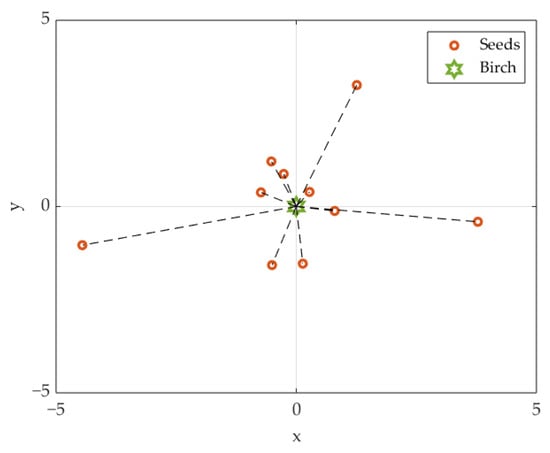
Figure 5.
Illustration of Levy flights of 10 seeds spread from a single birch.
The exploration of the optimization area in initial iterations of the algorithm is becoming the inevitable exploitation of the area around the best solution near the fittest specimen. This step coefficient adaptation is given in Equation (4).
where —maximum number of iterations; i—number of current iteration; and w—seed weight coefficient, . The seed weight coefficient affects the slope factor of the step coefficient, and heavy seeds are more likely to fall next to the parent tree—resulting in quicker exploitation of the current minima neighborhood. Thus, the parameter of the seed weight coefficient should be adopted for the considered problem in order to reduce false optimization in the local minimum. However, is also not recommended, as the coefficient remains constant during all iterations of the BiOA. Figure 6 presents exemplary values of the step coefficient for different w values and single random values. It is clear that the smaller the step is, the more the exploration of the search range decreases. The results presented in the further parts of the paper were obtained with a parameter set in the middle of the adaptation range.
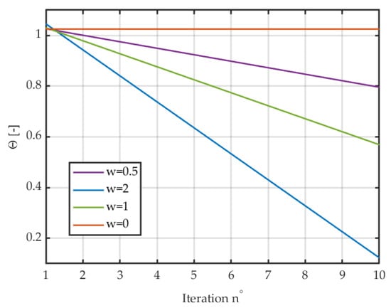
Figure 6.
Step coefficient in subsequent iterations of the BiOA.
The BiOA assumes that the seeds are produced by the fittest specimen; thus the new positions—corresponding to new solutions—are calculated according to (Equation (5)):
where —the fittest specimen in the i-th iteration.
The second part of the BiOA iteration is inspired by the growth process of birch trees. It is a common law of dendrology that organisms compete for sunlight and humidity. Therefore, the specimens that grow close to others tend to evolve into dwarf forms. In contrast, remote trees are able to gather the required amount of light, humidity, and nutrients to grow up to 40 m. The stem of the single tree develops to become robust to wind. These observations form the foundation of the second step in which trees and dwarf forms (bushes) are differentiated. Thus, the update of the current solution depends on two parameters: the distance to other specimens (l) and random weather conditions (). The differentiation of two groups of birches is possible after the calculation of fitness function with solutions determined in the first step. If the improvement is noted—i.e., relation (Equation (6)) is fulfilled—the specimen is considered a tree. If the obtained result is worse than the worst result of the tree in the previous iteration but still better than any obtained by bushes in the previous iteration (Equation (7)), the specimen is a dwarf plant.
where —fitness function value; and —single tree specimen from the previous iteration.
where —dwarf specimen from the previous iteration.
The above relations (given in Equations (6) and (7)) provide the possibility of finding the best solution for each population. The defined differentiation does not introduce additional threshold parameters; thus, the ease of implementation is ensured as the population will always be divided. This is especially crucial for the BiOA performance, as the fittest tree produces seeds. It is also important to note that growth parameters for the tree are clearly bigger than those applied to bushes. For the parallel version of the algorithm discussed, the fittest tree is chosen in every subpopulation and is then used for its validation.
The formula for updating both bushes and trees is similar and is defined by Equation (8). However, the parameters are different— is randomly generated for each group. It is also assumed that the optimization space—area available for birch growth—is decreasing in time, thus the corresponding influence of weather (Figure 7).
where —weather conditions parameter, calculated with the formula (Equation (9))
and —improvement factor defined by Equation (10):
where —birch tree solution; l—calculated as Euclidean distance (Equation (11)) between specimens in the i-th iteration.
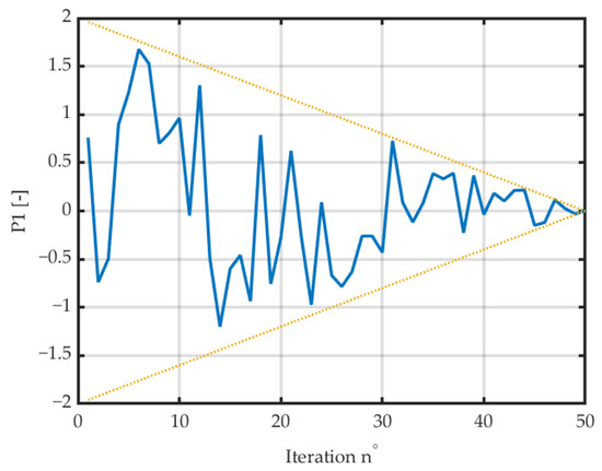
Figure 7.
Decreasing value of the weather condition parameter.
The decreasing character of the parameter is inspired by the constant growth of trees—access to roots is declining, as the ground cover is overlaid with enlarging crowns. Thus, the reduced access to rain can be observed and modeled accordingly. The linear decrease was chosen arbitrarily as similar functions are found in different NIOAs, e.g., the a parameter in GWO and time control in JSO [18,72]. The character of the decreasing function may be the subject of further improvements to the proposed algorithm.
where —considered specimen; d—dimension; and D—number of dimensions describing the task. All the parametrs of the BiOA are collected in Table 1.

Table 1.
Parameters of the BiOA and the suggested values.
The final solution obtained in the i-th iteration is similar to the process presented in Grey Wolf Optimizer [72]—the average position of the fittest specimens and dwarf trees is calculated (Equation (12)).
The obtained solutions are evaluated with the fitness function and the best solution is indicated. In the provided scenario, the optimization finishes after the designed number of iterations is computed. The process can be shortened by defining the stopping criteria based on the expected fitness function value.
The above subsequent calculations create a complete metaheuristic optimization algorithm. The flowchart including all the equations and operations forming the schematic of the BiOA is presented in Figure 8.
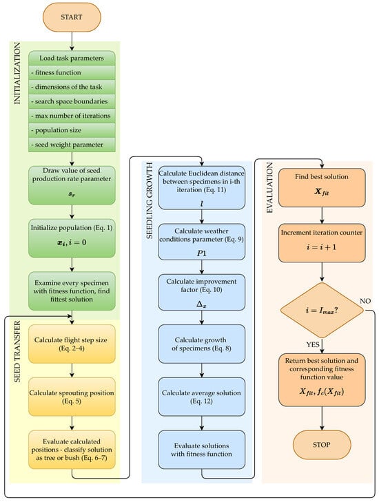
Figure 8.
Flow chart of the BiOA.
3. Results
3.1. Benchmark Functions
Every optimization algorithm requires examination to confirm its ability to find global minimum solutions. A properly functioning optimizer is able to explore optimization space thoroughly and avoid finding local minimum solutions. This property is the most important characteristic of any optimizer and needs to be proven with synthetic optimization tasks. These tasks are called benchmark functions [73,74,75] and include multidimensional problems with problematic solutions (local minima) defined within given optimization bounds.
3.1.1. Michalewicz Function
The efficacy of the developed optimization algorithm (BiOA) was tested with the Michalewicz benchmark function. The Michalewicz function is a multimodal with d dimensions. The number of local minima is also defined and equals , which makes the optimization task more complicated [76]. The function is expressed with the formula (Equation (13)):
where: d—number of dimensions; m—“steepness” parameter, usually .
The function is evaluated within a hypercube restricted by the relation (Equation (14)):
The chosen benchmark function is especially complicated for optimization algorithms because of the defined number of local minima and the shape of the function’s surface—compiled of ridges and valleys (it can be noted in function graph for presented in Figure 9).
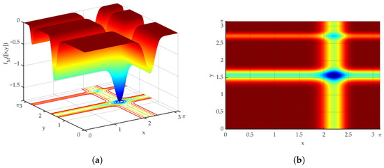
Figure 9.
Graph of Michalewicz function defined for : 3D view of the function (a), heat map of the function—view from the top (b).
The value of global minimum of the function defined for chosen d dimensions is gathered in a Table 2.
Table 2.
Chosen global minima of Michalewicz benchmark function [77].
The evaluation of the two-dimensional Michalewicz function was the crucial test for the BiOA. The examination considered a population of 20 specimens, while the number of iterations was adjusted. Obtained results are gathered in Table 3. Because of the known value of the optimal solution, it was possible to calculate the distance between the obtained result and the minimum.
Table 3.
Results of optimization of the Michalewicz function (, ) with BiOA.
It could be noted that all trials were successful—even the shortest optimization found a solution very close to the global minimum. Figure 10 presents all the best solutions obtained during optimization during 10 iterations, while Figure 11 presents convergence curves of the optimization process for different maximum iteration limits. The algorithm passed the test of evading the local minimum perfectly. Even though the reliability and efficacy of the BiOA were proved during the presented tests, further examination with the function defined within 5 and 10 dimensions was conducted.
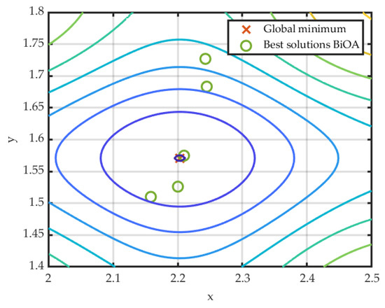
Figure 10.
Dispersion of the best results around the optimal result—10 iterations of BiOA.
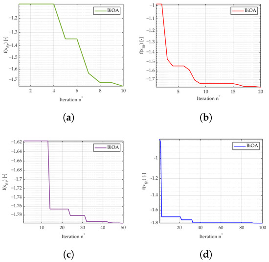
Figure 11.
Convergence curves for the subsequent test with different : (a), (b), (c), 100 (d).
The results presented in Table 4 confirm the correct operation of the algorithm. Additional observations can be made—for more complex optimization tasks, the number of iterations must be increased to obtain satisfactory results. Table 5 presents the results of a more complex 10-dimensional Michalewicz benchmark. Similarly to previous tests, the BiOA found solutions close to the global minimum shown in Table 2. The correlation between the maximum number of iterations and the distance to the global minimum is not linear, nevertheless, the trend of accuracy increase with optimization elongation can also be noted.
Table 4.
Results of optimization of the Michalewicz function (, ) with the BiOA.
Table 5.
Results of the optimization of the Michalewicz function (, ) with the BiOA.
3.1.2. Schaffer Function
The proposed algorithm was also tested with a Schaffer benchmark function [78], which is also a multimodal continuous two-dimensional () problem. It is characterized by the fact that the global minimum is placed close to the local minima [73]. The 2D problem is defined with the below formula (Equation (15)):
where . For the tests conducted, a limited search range was considered:
The graph of the Schaffer function is presented in Figure 12, and the wavy shape spreads around the global minimum located at , as shown in Table 6.
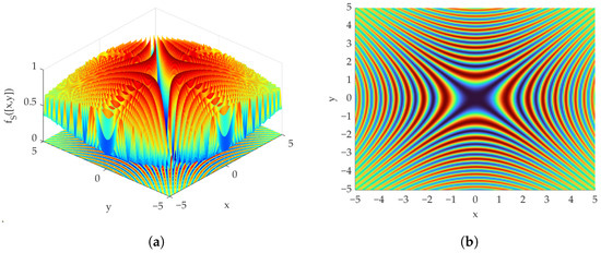
Figure 12.
Graph of a two-dimensional Schaffer function: 3D view of the function (a), heat map of the function—view from the top (b).
Table 6.
The global minimum of the Schaffer benchmark function [74].
The test conditions were similar to those presented in previous parts of the paper. Table 7 compiles the solution achieved by the BiOA and the distance to the global minimum (see Table 6 for the certified solution). The actual solutions are presented in Figure 13.
Table 7.
Results of optimization of the Schaffer function with the BiOA.
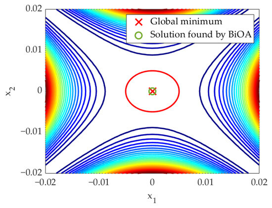
Figure 13.
Dispersion of the best results after 50 runs of BiOA; the satisfactory results are in the area marked within the red figure.
3.1.3. Ackley Function
The research included also the Ackley function, which is a convex function, defined by Equation (17) as a 2-dimensional problem in the range . It results in a funnel-like shape with a global minimum in the central hollow (Table 8).
where , , and .
Table 8.
The global minimum of the Ackley benchmark function [74].
Figure 14 presents the best solutions of the Ackley function obtained with 50 subsequent runs of the BiOA. The scale of the graph and the very precise convergence to the global minimum should be emphasized.
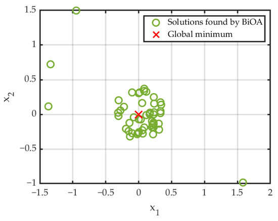
Figure 14.
Dispersion of best results after 50 runs of BiOA.
To reduce the complexity of the paper, the results were compiled into a Table 9 presented in the global performance assessment subsection.
Table 9.
Collation of the results obtained after 50 runs of different NIOAs and the Ackley benchmark function.
3.1.4. Performance Assessment
The results presented in previous subsections can be easily compared to performances of different NIOAs available in the literature [77,79]. However, to ensure the authenticity of the comparison, the research included an optimization of the benchmark functions (Section 3.1.1, Section 3.1.2 and Section 3.1.3) with a group of well-recognized NIOAs performed on the exact machine equipped with an eight 8-core AMD Ryzen CPU and 20 GB of RAM. The comparison included popular optimizers—it should be noted that the representatives from different periods of NIOAs development [80] have been tested: Particle Swarm Optimization (PSO) (1995), Artificial Bee Colony (ABC) (2007), Flower Pollination Algorithm (FPA) (2012), Grey Wolf Optimizer (GWO) (2014), Jellyfish Search Optimizer (JSO) (2021), and Chameleon Swarm Algorithm (CSA) (2021). All examined algorithms were configured with default parameters (Table A1). The clarification and the influence of different parameters on adequate algorithms can be found in the literature.
It can be assumed that having too many parameters reduces the ease of the algorithm’s application. However, the tunable parameters should not be neglected to ensure control over algorithm dynamics. Thus, the authors recognized the FPA and the BiOA as a good balance between configuration ability and application effort.
The most crucial indicator of algorithm performance is convergence to the global minimum. Thus, Figure 15 and Figure 16 present the distribution of the best solutions () around the global minimum calculated in 50 independent runs, while all the corresponding indicators are gathered in Table 10 and Table 11.
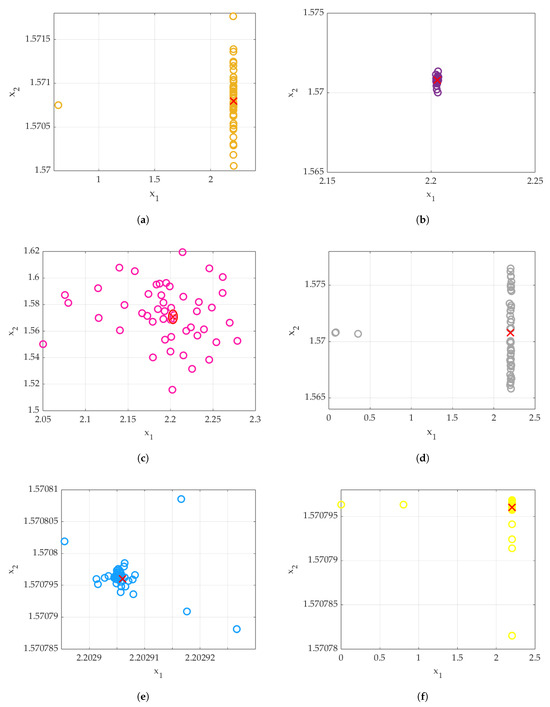
Figure 15.
Distribution of the best solutions in subsequent tests of the 2D Michalewicz function for different NIOAs around global minimum (×): PSO (a), ABC (b), FPA (c), GWO (d), JSO (e), and CSA (f).
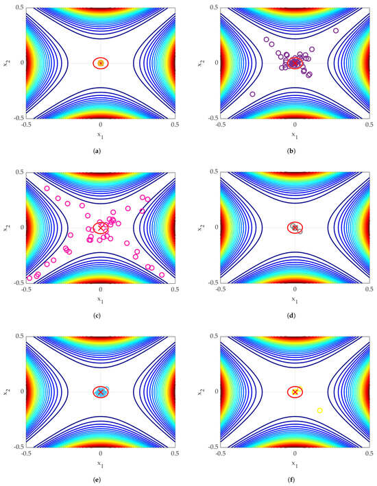
Figure 16.
Distribution of the best solutions in subsequent Schaffer benchmark runs for different NIOAs around the global minimum (×): PSO (a), ABC (b), FPA (c), GWO (d), JSO (e), and CSA (f).
Table 10.
Collation of the results obtained after 50 runs of different NIOAs and the Michalewicz benchmark function.
Table 11.
Collation of the results obtained after 50 runs of different NIOAs and the Schaffer benchmark function.
Figure 17 presents statistics regarding Shaffer benchmark runs with different optimizers. It could be noted that generally, all tested algorithms ensured satisfactory results—the mean value achieved with all algorithms is placed close to the global minimum (with a negligible shift <0.0005). However, the FPA and the CSA were characterized by reduced repeatability. The distribution of the results achieved with the CSA is uneven with a high variance—as can be observed in both Figure 17 and Figure 18. The densest distribution around the global minimum was obtained with the PSO, the GWO, the JSO, and the BiOA (Figure 17).
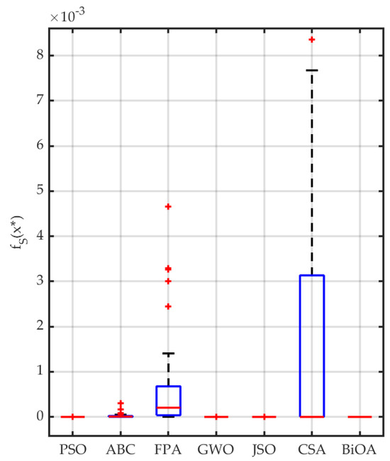
Figure 17.
Boxplot of the Schaffer function value distribution after 50 runs with different NIOAs.
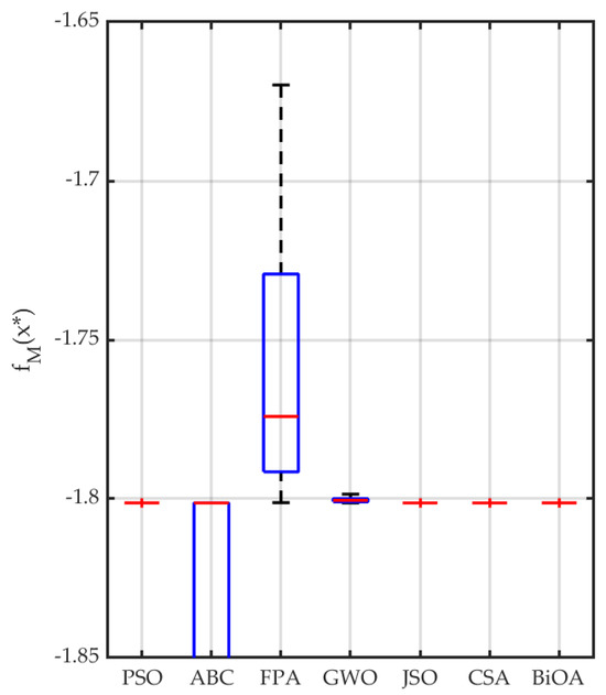
Figure 18.
Boxplot of the Michalewicz function value distribution after 50 runs with different NIOAs.
The tests with the Ackley benchmark function confirmed again the high precision of the BiOA. Not only were all the results gathered close to the global minimum but also the variance for the representative group was characterized by a negligible value. This can also be noted from the boxplot in Figure 19. The remaining statistics of the test runs with the Ackley function with all chosen optimizers are presented in Table 9.
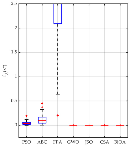
Figure 19.
Boxplot of the Ackley function value distribution after 50 runs with different NIOAs.
Finally, for simple comparison purposes, the complexity parameter (—optimizer complexity) was introduced. It indicates a number of direct calculations required by a single iteration of the optimizer. Thus, the smaller the value, the less complicated and the more power-efficient algorithm is. The complexity parameters are gathered in Table 12.
Table 12.
Comparison of the optimization algorithm’s computational complexity and average computation times of an optimization for the evaluated benchmark functions.
It could be noted that the complexity index, which equals the number of required calculations, may not be an adequate indicator because of the different compilation times of different mathematical operations. It can be noted that the algorithms are organized in a table based on the presentation date. Thus, it can be noted that the optimization time has decreased by about since the development of pioneering algorithms.
3.2. Real-Life Applications
3.2.1. Bin-Packing Problem
The planning based on optimization is often applied for the placement of the elements on the closed area. It often deals with car-parking problems or the packing of different-size elements. It is a complex task and is widely analyzed and described in scientific papers [81,82,83,84,85,86]. One of the mentioned problems was used as benchmark for the proposed BiOA algorithm. The goal of the calculations was focused on packing different-size elements (vehicles) in a closed area (parking). The task was defined to fit the maximum number of predefined boxes, 30, into a rectangle. The group was randomly generated at the beginning of tests. The test is based on the modification of the problem defined by Maxim Vedenyov [87]. The boxes may be rotated and replaced among the given group to fill the maximum percentage of the available area. The results are presented in Figure 20.
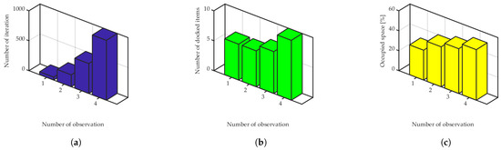
Figure 20.
Results of the BiOA application for the parking/packing task: number of iterations (a), number of docked items (b), filled space (c).
The selected characteristic four points of the optimization process are shown in the bar plots (Figure 20). The following stages of calculations are noted (Figure 20a). The maximum number of iterations is defined as 1000. During the optimization, the number of the docked elements is growing (each defined object is placed) as the filled area is simultaneously being expanded (related to the box size parked without collision). The results presented above confirm that the BiOA can be also applied to the fitting optimization task.
3.2.2. Engineering Application
The successful synthetic test with a benchmark function proved the efficiency of the BiOA. Thus, the next step of algorithm validation could be investigated. The second application of the BiOA optimizer deals with a real-life engineering problem related to the design of a speed control structure applied to an electrical drive. The unique construction is considered, and the motor and the load are connected using long elastic coupling (Figure 21). It is a source of state variable oscillations. Under the described conditions, precise speed control is difficult.
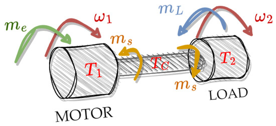
Figure 21.
Scheme of the two-mass system.
The implemented control system is mainly based on the PI controller. However, for the efficient damping of torsional vibrations, additional feedback paths are used [46]. The first is related to the difference between motor speed and load speed . The next one is from the shaft torque . The schematic diagram is presented in Figure 22. A system with an extended mechanical part is considered (Equation (18)):
where and are the speed of the motor and speed of the system output, respectively; is the shaft torque; is an electromagnetic torque; and , and are mechanical time constants of the motor, the load and an shaft, respectively. The parameters’ values are presented in a Table 13.
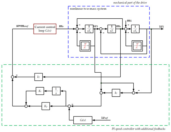
Figure 22.
Speed control structure—based on a PI controller and additional feedback connections from shaft torque and speeds—applied to a two-mass system.
Table 13.
Geometric and dynamic parameters of the system.
The internal part (PI current controller, sensors, power electronics, etc.) can be described using the formula
where is the equivalent current loop time constant. In some cases, assuming much faster processing of the internal part (compared to a speed control loop with mechanical time constants), the simplification can be introduced: s.
Let us consider in the first part of the considerations, a linear object. According to the analytical approach, using the pole placement method to calculate the parameters of the speed controller, the transmittance from the output to the input is necessary:
obviously, the (Equation (21)) represents the PI controller:
Comparing the characteristic equation of the analyzed system and the desired polynomial of the control structure, the equations describing the values of the controller gains can be determined:
where —resonant frequency, —damping coefficient. The transmittance of the system (Equation (20)) contains a term in the numerator. Thus, the overshoots can be observed. For this purpose, in order to reduce the mentioned phenomenon, the input filter is applied (Equation (26)):
The presented equations prove the strict dependence of the gain coefficients of the control system (the main PI controller and feedback gains) on the values of the time constants of the object. However, after the precise identification and invariance of the two-mass system parameters, it can be an efficient control method.
The purpose of the above analytical analysis of the control structure was also to analyze stability. Figure 23 presents the positions of poles and zeros achieved for the analyzed system, which were plotted based on the transmittance of a closed-loop system (Equation (20)). The poles are placed on the left side of the S-plane. It leads to an obvious conclusion—the system is stable. The numerator of the transmittance includes the ‘s’. It is related to the zeros; in a real application, the overshoots should be damped using an input filter.
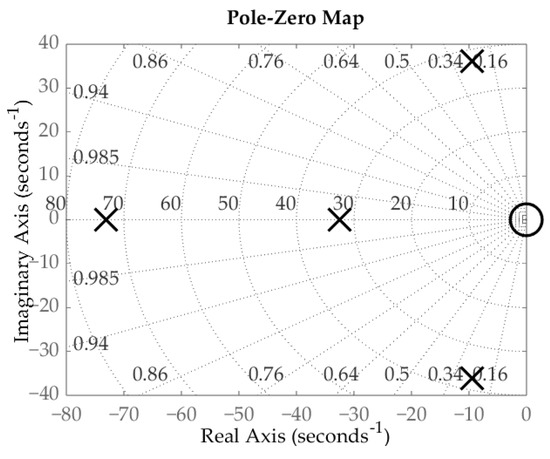
Figure 23.
Root locus of the system optimized using the BiOA algorithm.
It should be noted that the analysis presented above is quite simple for a linear model of the mechanical part. However, in real objects, there are a number of factors whose occurrence makes the use of analytical expressions suboptimal. These include possible nonlinearities, including friction localized on the side of the drive motor and the working machine or nonlinear characteristics of the mechanical shaft. Another factor is the variability of object parameters during operation. In the case of the drive train, this is the time constant of the working machine. Since analytical expressions depend directly on the parameters of the drive system, their application in such a case is problematic. For this reason, other approaches are sought. In this article, a new metaheuristic algorithm is used to select the parameters of the control structure.
Initially, a cost function has to be defined. For the considered task, a simple two-component function was chosen to correctly trace and reduce the influence of the elastic connection. Thus, the cost function (Equation (27)) based on motor speed, load speed, and the reference value was defined. The shape of the cost function may be adapted to the requirements defined for the considered optimization task. In the case of two-mass systems, simple linear functions are the most popular [51,72,88]; however, more complex quadratic or Huber functions may also be applied [36,89,90]. For the given system, for example, electromagnetic torque () may also be shaped. However, in such cases, it is a good practice to implement weighting coefficients to prioritize each element of the cost function. Nevertheless, it should be emphasized that such a multiobjective approach is always a consensus of the optimum of every individual parameter.
where N—total number of considered samples; n—sample counter; and —output of the reference model with designed dynamics given with a second-order system transfer function (Equation (28)).
The optimization task in this part was a four-dimensional problem—four coefficients of the speed controller () were searched. The optimization with the BIOA was successful and resulted in a smooth speed transience without conspicuous oscillation and overshoot (Figure 24). Thus, it was confirmed empirically that the developed BiOA can also be used in real-life optimization problems.
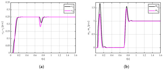
Figure 24.
Transients of a two-mass system with PI speed controller optimized with the BiOA, motor, and load speeds: (a), electromagnetic torque (b).
For comparison purposes, the same system was also optimized with the NIOAs examined with synthetic benchmark-based tests presented in the previous parts of the paper, Section 3. Thus the PSO, the ABC, the FPA, the GWO, the JSO, and the CSA were also considered in this part. All optimizations were executed with default values of parameters and the defined population size: 20 specimens. Every iteration included a simulation of the 4-s operation of a two-mass system. To ensure comparability and credibility of the obtained results, the initial population was randomly drawn only once and reused in subsequent runs. The tests were conducted on a PC equipped with an 8-core AMD Ryzen CPU and 20 GB of RAM. The results are gathered in Table 14. Figure 25 and Figure 26 confirm that all tested NIOAs converge on similar values.
Table 14.
Comparison of optimization results for different NIOAs—parameters of the speed controller for a two-mass system.
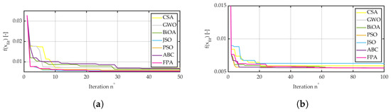
Figure 25.
Convergence curves of best results obtained during optimization with different NIOAs, 50 iterations (a), 100 iterations (b).
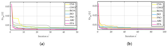
Figure 26.
Average convergence curves of 5 subsequent optimizations with different NIOAs: 50 iterations (a), 100 iterations (b).
For comparison reasons, we decided to present both the best result convergence curve and the average result calculated for five runs. The proper initialization was used, and every algorithm used identical starting points, which can be clearly seen in Figure 26.
The second part of the simulation tests included the verification of multiobjective optimization. For this purpose, the original cost function (Equation (27)) was extended with the second objective (Equation (29)). Additionally, the weighting coefficients were implemented to prioritize speed control over torque.
where —electromagnetic torque and —load torque.
The results of this extended test can be seen in Figure 27. As was assumed, the multiobjective optimization can also be conducted with the BiOA. However, also according to expectations, the multiobjective task allowed a reduction in torque overshoot, which resulted in worse dynamics observed in speed transience. This can be especially observed at 0.8 s—a moment when load torque is applied. Thus, the previously drawn foresight was proven.
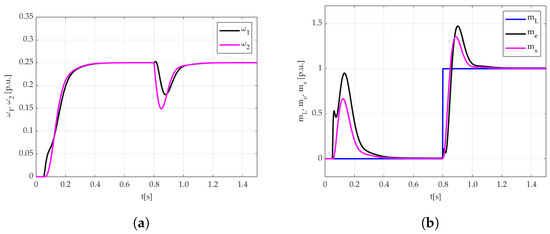
Figure 27.
Transients of two-mass system state variables optimized with the BiOA and multiobjective cost function, motor and load speeds (a), and electromagnetic torque (b).
The applicability and simulation results were also tested with experimental test results. The initial test (Figure 28) included the structure with controller parameters calculated with analytical formulas. In the second step, the control structure and the optimized coefficients were considered (Figure 29). The implementation of the considered control structure complied with the PI speed controller, and additional feedback on the torque and speed difference between the motor and load machine was performed with the dSPACE workbench. The Simulink model was compiled and loaded to the controller connected to the power electronics of the two-mass stand. The transients of the state variables were plotted during the experiment with ControlDesk software. Figure 30 presents the laboratory stand used during the experiment.
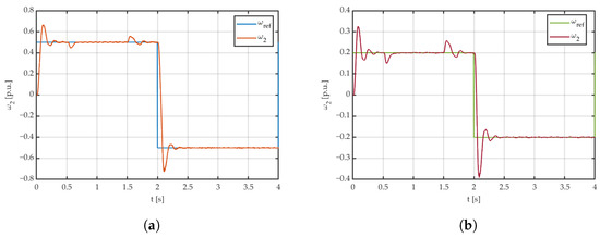
Figure 28.
Transients of the load speed () achieved with calculated coefficients—experiment ( (a), (b)).
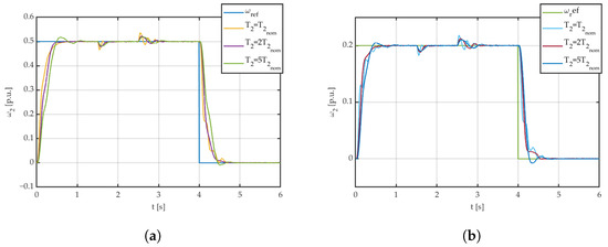
Figure 29.
Transients of the load speed () achieved with parameters optimized with BiOA—experiment ( (a), (b)).
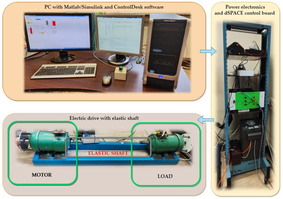
Figure 30.
The laboratory bench used in the experiment.
The system with coefficients chosen using analytical expressions was tested first. A value lying in the middle of all possible values—the average value—was taken as the parameter in the mathematical equations. As can be seen from the analysis of the obtained results, the speed of the working machine contains a large overshoot. This is due to the adoption of an incorrect value of the constant in the analytical method. Subsequently, a meta-heuristic algorithm with parameters as in the simulation studies was used to select the coefficients of the control system. After the optimization process, constant settings of the control system were obtained to ensure similar speed trajectories of the working machine for different values of . The experimental test plan was as follows. The system with the rated parameters was tested first. Subsequently, rotating masses were added to the set, increasing the moment of inertia in the working machine. Then, the tests were repeated for 2 and 5 times the increasing time constant, respectively.
Figure 29 shows the aggregate transients of the working machine for different values of mechanical time constants. At time = 0 s, the system is started. Subsequently, at = 1.5 s, a rated load torque is applied to the system, which is taken off at = 2.5 s. As can be seen from the summary analysis in Figure 29, the speed waveforms are similar. In the case of a five-fold increase in the time constant of the load machine, a slight overshoot of about 6% can be observed. In other cases, there is no overshoot. It is also possible to note the different responses of the system under changes in the load torque. These are due to the different values of the moment of inertia.
4. Discussion
The crucial point of the paper is the presentation of a novel optimization algorithm based on birch tree succession behavior. The BiOA introduced is supported by an extended comparison of the performance with a couple of benchmark tests. Referring to the presented results, observations and findings may be formulated as follows.
- The developed BiOA resulted in a very high precision in convergence toward the global minimum. This is caused by the parameters decreasing with the next iterations. Thus, it was observed that the BiOA was able to achieve results with even accuracy. None of the compared algorithms was characterized by such perfect results.
- An analysis of the results compiled with optimization time clearly indicates the increase in performance of the modern NIOAs. Surprisingly, the results achieved with a very popular optimizer—the ABC—were unsatisfactory. This might have been caused by the default values of algorithm parameters.
- Based on the above observations, an additional statement may be drawn: modern algorithms (except the CSA) are characterized by a reduced number of tunable parameters. This makes the application of NIOAs a simple and convenient tool.
- The performance of any algorithm should be paired with a satisfactory optimization time. The development of NIOAs (based on the chosen representatives) has significantly decreased the optimization time of benchmark functions. In this field, the JSO performed best; however, the number of adjustable parameters is rather high. This may lead to substantially longer and more difficult implementation. In the case of engineering applications, the optimization time is negligible with respect to the simulation time.
Additionally, this article presents issues related to the design of a control structure for an elastic-joint drive system that is resistant to changes in object parameters. Based on theoretical considerations confirmed by simulation and experimental studies, the final remarks presented below can be made.
- In order to effectively dampen torsional vibrations with an elastic connection, one of the advanced control structures should be used. In the present study, a system with a PI controller and additional couplings from the torsional torque and speed difference between the working motor and the load machine was chosen. For a system with known and fixed parameters, it is possible to use the pole placement method to select the parameters of the control system and achieve the assumed pole location of the closed system. This provides the desired trajectories of closed-loop system state variables in the linear range of operation.
- If there are significant nonlinearities in the system and/or changes in the system parameters during operation, the use of the pole placement method is not optimal. This technique requires the actual parameters of the system—their change causes a change in the location of the poles of the closed system. This can result in large overshoots in the system or a significant increase in rising time.
5. Conclusions
In this paper, a new optimization method based on birch succession is proposed. It is characterized by typical optimization properties of algorithms noticed in the literature. It finds the minimum of the objective function in a short time. However, the faster execution time of the calculations compared to other tested algorithms should be noted. The application of metaheuristic methods ensures the optimal selection of parameters of the control structure in accordance with the defined objective function. In the present study, it was possible to select parameters in this way, resulting in similar speed courses of the working machine despite the different values of the working machine’s moment of inertia. Nature-inspired optimization algorithms are able to find values close to the global minimum. The observed accuracy is satisfactory for most applications. The mathematical operations required by the NIOAs are less complicated in comparison to gradient methods, explaining the increasing popularity of such algorithms.
Because of noticed behavior, future work on the issues addressed in this paper will focus on the following two issues.
- An analysis of control structures in terms of their robustness to changes in object parameters. Special attention will be paid to structures that are a combination of input shaping techniques and selected closed-loop control structures. A detailed verification of the effect of cost function order for optimization on system dynamics will be also conducted.
- Further development of the birch tree succession algorithm. We plan to introduce subpopulations and migration patterns between them. This is especially important for parallel processing offered by modern processors. This will ensure further shortening of the optimization process.
Author Contributions
Conceptualization, M.K., S.K., M.M. and K.S.; methodology, M.K., S.K., M.M. and K.S.; software, M.M.; validation, M.K. and K.S.; formal analysis, M.K., S.K., M.M. and K.S.; investigation, M.K., S.K., M.M. and K.S.; data curation, M.M. and M.K.; writing—original draft preparation, M.K., S.K., M.M. and K.S.; writing—review and editing, M.K., S.K., M.M. and K.S.; visualization, M.K., M.M. and K.S.; supervision, M.K. and K.S.; project administration, M.K. and K.S. All authors have read and agreed to the published version of the manuscript.
Funding
This research received no external funding.
Data Availability Statement
The data are contained within the article.
Conflicts of Interest
The authors declare no conflicts of interest.
Abbreviations
The following abbreviations and symbols are used in this manuscript:
| AI | Artificial Intelligence |
| ABC | Artificial Bee Colony |
| ACO | Ant Colony Optimization Algorithm |
| DO | Dandelion Optimizer |
| FPA | Flower Pollination Algorithm |
| GWO | Grey Wolf Optimizer |
| CSA | Chameleon Swarm Algorithm |
| BiOA | Birch-inspired Optimization Algorithm |
| PSO | Particle Swarm Optimizer |
| WOA | Whale Optimization Algorithm |
| JSO | Jellyfish Search Optimizer |
| FDC | Forced Dynamic Control |
| MPC | Model Predictive Control |
| NIOA | Nature inspired optimization algorithm |
| seed production rate | |
| shaft torque | |
| electromagnetic torque | |
| load torque | |
| motor time constant | |
| load machine time constant | |
| shaft time constant | |
| speed of motor | |
| speed of load |
Appendix A
In order to ensure reproducibility of the research, the default parameters for the examined NIOAs were applied. These values are gathered in Table A1.
Table A1.
Default parameters of the examined NIOAs.
Table A1.
Default parameters of the examined NIOAs.
| PSO | ABC | FPA | GWO | JSO | CSA | BiOA |
|---|---|---|---|---|---|---|
References
- Pham, T.H.; Raahemi, B. Bio-Inspired Feature Selection Algorithms with Their Applications: A Systematic Literature Review. IEEE Access 2023, 11, 43733–43758. [Google Scholar] [CrossRef]
- Roni, M.H.K.; Rana, M.S.; Pota, H.R.; Hasan, M.M.; Hussain, M.S. Recent trends in bio-inspired meta-heuristic optimization techniques in control applications for electrical systems: A review. Int. J. Dyn. Control. 2022, 10, 999–1011. [Google Scholar] [CrossRef]
- Kulejewski, J.; Rosłon, J. Optimization of Ecological and Economic Aspects of the Construction Schedule with the Use of Metaheuristic Algorithms and Artificial Intelligence. Sustainability 2023, 15, 890. [Google Scholar] [CrossRef]
- Liu, M.; Shin, D.; Kang, H.I. Parameter estimation in dynamic biochemical systems based on adaptive Particle Swarm Optimization. In Proceedings of the 2009 7th International Conference on Information, Communications and Signal Processing (ICICS), Macau, China, 8–10 December 2009; pp. 1–5. [Google Scholar] [CrossRef]
- Jakšić, Z.; Devi, S.; Jakšić, O.; Guha, K. A Comprehensive Review of Bio-Inspired Optimization Algorithms Including Applications in Microelectronics and Nanophotonics. Biomimetics 2023, 8, 278. [Google Scholar] [CrossRef] [PubMed]
- Jayashree, R. Preventing the Early Spread of Infectious Diseases Using Particle Swarm Optimization. In Nature-Inspired Optimization Methodologies in Biomedical and Healthcare; Springer International Publishing: Cham, Switzerland, 2023; pp. 33–47. [Google Scholar] [CrossRef]
- Suguna, S.K.; Ranganathan, R.; Sangeetha, J.; Shandilya, S.; Shandilya, S.K. Application of Nature—Inspired Algorithms in Medical Image Processing. In Advances in Nature-Inspired Computing and Applications; Springer: Cham, Switzerland, 2018. [Google Scholar]
- Su, H.; Zhao, D.; Heidari, A.A.; Liu, L.; Zhang, X.; Mafarja, M.; Chen, H. RIME: A physics-based optimization. Neurocomputing 2023, 532, 183–214. [Google Scholar] [CrossRef]
- Biswas, A.; Mishra, K.K.; Tiwari, S.; Misra, A.K. Physics-Inspired Optimization Algorithms: A Survey. J. Optim. 2013, 2013, 438152. [Google Scholar] [CrossRef]
- Henderson, D.; Jacobson, S.H.; Johnson, A.W. The Theory and Practice of Simulated Annealing. In Handbook of Metaheuristics; Springer: New York, NY, USA, 2003; pp. 287–319. [Google Scholar] [CrossRef]
- Salehan, A.; Deldari, A. Corona virus optimization (CVO): A novel optimization algorithm inspired from the Corona virus pandemic. J. Supercomput. 2022, 78, 5712–5743. [Google Scholar] [CrossRef]
- Zhang, Z. A new Hybrid Infection model optimization Algorithm. In Proceedings of the 3rd International Conference on Material, Mechanical and Manufacturing Engineering, Guangzhou, China, 27–28 June 2015; pp. 1045–1050. [Google Scholar] [CrossRef]
- Farrag, T.A.; Farag, M.A.; Rizk-Allah, R.M.; Hassanien, A.E.; Elhosseini, M.A. An improved parallel processing-based strawberry optimization algorithm for drone placement. Telecommun. Syst. 2023, 82, 245–275. [Google Scholar] [CrossRef]
- Zhao, S.; Zhang, T.; Ma, S.; Chen, M. Dandelion Optimizer: A nature-inspired metaheuristic algorithm for engineering applications. Eng. Appl. Artif. Intell. 2022, 114, 105075. [Google Scholar] [CrossRef]
- Bidar, M.; Kanan, H.R.; Mouhoub, M.; Sadaoui, S. Mushroom Reproduction Optimization (MRO): A Novel Nature-Inspired Evolutionary Algorithm. In Proceedings of the 2018 IEEE Congress on Evolutionary Computation (CEC), Rio de Janeiro, Brazil, 8–13 July 2018; pp. 1–10. [Google Scholar] [CrossRef]
- Nagy, Z.; Werner-Stark, A.; Dulai, T. An Artificial Bee Colony Algorithm for Static and Dynamic Capacitated Arc Routing Problems. Mathematics 2022, 10, 2205. [Google Scholar] [CrossRef]
- Mavrovouniotis, M.; Anastasiadou, M.N.; Hadjimitsis, D. Measuring the Performance of Ant Colony Optimization Algorithms for the Dynamic Traveling Salesman Problem. Algorithms 2023, 16, 545. [Google Scholar] [CrossRef]
- Chou, J.S.; Molla, A. Recent advances in use of bio-inspired jellyfish search algorithm for solving optimization problems. Sci. Rep. 2022, 12, 19157. [Google Scholar] [CrossRef] [PubMed]
- Precup, R.E.; David, R.C.; Szedlak-Stinean, A.I.; Petriu, E.M.; Dragan, F. An Easily Understandable Grey Wolf Optimizer and Its Application to Fuzzy Controller Tuning. Algorithms 2017, 10, 68. [Google Scholar] [CrossRef]
- Elliott, W.M.; Wyman, R.L.; Elliott, N.B. Significance of Living Records. Bios 1984, 55, 211–218. [Google Scholar]
- Darvishpoor, S.; Darvishpour, A.; Escarcega, M.; Hassanalian, M. Nature-Inspired Algorithms from Oceans to Space: A Comprehensive Review of Heuristic and Meta-Heuristic Optimization Algorithms and Their Potential Applications in Drones. Drones 2023, 7, 427. [Google Scholar] [CrossRef]
- Kumar, A.; Nadeem, M.; Banka, H. Nature inspired optimization algorithms: A comprehensive overview. Evol. Syst. 2023, 14, 141–156. [Google Scholar] [CrossRef]
- Zakeri, H.; Nejad, F.M.; Gandomi, A.H. Nature-Inspired Optimization Algorithms (NIOAs). In Automation and Computational Intelligence for Road Maintenance and Management; Chapter 10; John Wiley and Sons, Ltd.: Hoboken, NJ, USA, 2022; pp. 437–474. [Google Scholar] [CrossRef]
- Yang, X.S. Nature-Inspired Optimization Algorithms, 2nd ed.; Academic Press: Cambridge, MA, USA, 2021. [Google Scholar] [CrossRef]
- Larik, A.S.; Haider, S. A survey of nature inspired optimization algorithms applied to cooperative strategies in robot soccer. In Proceedings of the 2018 International Conference on Advancements in Computational Sciences (ICACS), Lahore, Pakistan, 19–21 February 2018; pp. 1–6. [Google Scholar] [CrossRef]
- Rai, R.; Das, A.; Dhal, K.G. Nature-inspired optimization algorithms and their significance in multi-thresholding image segmentation: An inclusive review. Evol. Syst. 2022, 13, 889–945. [Google Scholar] [CrossRef] [PubMed]
- Dhal, K.G.; Das, A.; Ray, S.; Galvez, J.; Das, S. Nature-inspired optimization algorithms and their application in multi-thresholding image segmentation. Arch. Comput. Methods Eng. 2020, 27, 855–888. [Google Scholar] [CrossRef]
- Prach, K.; Pyšek, P. Using spontaneous succession for restoration of human-disturbed habitats: Experience from Central Europe. Ecol. Eng. 2001, 17, 55–62. [Google Scholar] [CrossRef]
- Van der Burght, L.; Stoffel, M.; Bigler, C. Analysis and modelling of tree succession on a recent rockslide deposit. Plant Ecol. 2012, 213, 35–46. [Google Scholar] [CrossRef]
- Jonczak, J.; Oktaba, L.; Pawłowicz, E.; Chojnacka, A.; Regulska, E.; Słowińska, S.; Olejniczak, I.; Oktaba, J.; Kruczkowska, B.; Kondras, M.; et al. Soil organic matter transformation influenced by silver birch (Betula pendula Roth) succession on abandoned from agricultural production sandy soil. Eur. J. For. Res. 2023, 142, 367–379. [Google Scholar] [CrossRef]
- Gasiyarov, V.R.; Radionov, A.A.; Loginov, B.M.; Zinchenko, M.A.; Gasiyarova, O.A.; Karandaev, A.S.; Khramshin, V.R. Method for Defining Parameters of Electromechanical System Model as Part of Digital Twin of Rolling Mill. J. Manuf. Mater. Process. 2023, 7, 183. [Google Scholar] [CrossRef]
- Zawirski, K.; Brock, S.; Nowopolski, K. Recursive Neural Network as a Multiple Input and Multiple Output Speed Controller for Electrical Drive of Three-Mass System. Energies 2024, 17, 172. [Google Scholar] [CrossRef]
- Liu, Y.; Song, B.; Zhou, X.; Gao, Y.; Chen, T. An Adaptive Torque Observer Based on Fuzzy Inference for Flexible Joint Application. Machines 2023, 11, 794. [Google Scholar] [CrossRef]
- Serkies, P.; Gorla, A. Implementation of PI and MPC-Based Speed Controllers for a Drive with Elastic Coupling on a PLC Controller. Electronics 2021, 10, 3139. [Google Scholar] [CrossRef]
- Łuczak, D. Mathematical model of multi-mass electric drive system with flexible connection. In Proceedings of the 2014 19th International Conference on Methods and Models in Automation and Robotics (MMAR), Miedzyzdroje, Poland, 2–5 September 2014; pp. 590–595. [Google Scholar] [CrossRef]
- Szczepanski, R.; Kaminski, M.; Tarczewski, T. Auto-Tuning Process of State Feedback Speed Controller Applied for Two-Mass System. Energies 2020, 13, 3067. [Google Scholar] [CrossRef]
- Wang, D.; Zhang, S.; Wang, L.; Liu, Y. Developing a Ball Screw Drive System of High-Speed Machine Tool Considering Dynamics. IEEE Trans. Ind. Electron. 2022, 69, 4966–4976. [Google Scholar] [CrossRef]
- Wang, L.; Han, J.; Ma, F.; Li, X.; Wang, D. Accuracy design optimization of a CNC grinding machine towards low-carbon manufacturing. J. Clean. Prod. 2023, 406, 137100. [Google Scholar] [CrossRef]
- Chen, L.; Du, X.; Hu, B.; Blaabjerg, F. Drivetrain Oscillation Analysis of Grid Forming Type-IV Wind Turbine. IEEE Trans. Energy Convers. 2022, 37, 2321–2337. [Google Scholar] [CrossRef]
- Zhang, X.; Huang, Y.; Wang, S.; Meng, W.; Li, G.; Xie, Y. Motion planning and tracking control of a four-wheel independently driven steered mobile robot with multiple maneuvering modes. Front. Mech. Eng. 2021, 16, 504–527. [Google Scholar] [CrossRef]
- Yamada, S.; Fujimoto, H. Precise Joint Torque Control Method for Two-inertia System with Backlash Using Load-side Encoder. IEEJ J. Ind. Appl. 2019, 8, 75–83. [Google Scholar] [CrossRef]
- Li, P.; Wang, L.; Zhong, B.; Zhang, M. Linear Active Disturbance Rejection Control for Two-Mass Systems Via Singular Perturbation Approach. IEEE Trans. Ind. Inform. 2022, 18, 3022–3032. [Google Scholar] [CrossRef]
- Sakaino, S.; Kitamura, T.; Mizukami, N.; Tsuji, T. High-Precision Control for Functional Electrical Stimulation Utilizing a High-Resolution Encoder. IEEJ J. Ind. Appl. 2021, 10, 124–133. [Google Scholar] [CrossRef]
- Yang, T.; Xu, F.; Zhao, S.; Li, T.; Yang, Z.; Wang, Y.; Liu, Y. A High-Certainty Visual Servo Control Method for a Space Manipulator with Flexible Joints. Sensors 2023, 23, 6679. [Google Scholar] [CrossRef] [PubMed]
- Sasaki, M.; Muguro, J.; Njeri, W.; Doss, A.S.A. Adaptive Notch Filter in a Two-Link Flexible Manipulator for the Compensation of Vibration and Gravity-Induced Distortion. Vibration 2023, 6, 286–302. [Google Scholar] [CrossRef]
- Szabat, K.; Orlowska-Kowalska, T. Vibration Suppression in a Two-Mass Drive System Using PI Speed Controller and Additional Feedbacks—Comparative Study. IEEE Trans. Ind. Electron. 2007, 54, 1193–1206. [Google Scholar] [CrossRef]
- Katsura, S.; Ohnishi, K. Force Servoing by Flexible Manipulator Based on Resonance Ratio Control. IEEE Trans. Ind. Electron. 2007, 54, 539–547. [Google Scholar] [CrossRef]
- Kobayashi, H.; Katsura, S.; Ohnishi, K. An Analysis of Parameter Variations of Disturbance Observer for Motion Control. IEEE Trans. Ind. Electron. 2007, 54, 3413–3421. [Google Scholar] [CrossRef]
- Stanislawski, R.; Tapamo, J.R.; Kaminski, M. Virtual Signal Calculation Using Radial Neural Model Applied in a State Controller of a Two-Mass System. Energies 2023, 16, 5629. [Google Scholar] [CrossRef]
- Serkies, P.; Szabat, K. Effective damping of the torsional vibrations of the drive system with an elastic joint based on the forced dynamic control algorithms. J. Vib. Control 2019, 25, 2225–2236. [Google Scholar] [CrossRef]
- Wróbel, K.; Śleszycki, K.; Kahsay, A.H.; Szabat, K.; Katsura, S. Robust Speed Control of Uncertain Two-Mass System. Energies 2023, 16, 6231. [Google Scholar] [CrossRef]
- Wang, C.; Liu, F.; Xu, J.; Pan, J. An SMC-Based Accurate and Robust Load Speed Control Method for Elastic Servo System. IEEE Trans. Ind. Electron. 2024, 71, 2300–2308. [Google Scholar] [CrossRef]
- Chang, H.; Lu, S.; Huang, G.; Zheng, S.; Song, B. An Extended Active Resonance Suppression Scheme Based on a Dual-Layer Network for High-Performance Double-Inertia Drive System. IEEE Trans. Power Electron. 2023, 38, 13717–13729. [Google Scholar] [CrossRef]
- Jastrzębski, M.; Kabziński, J.; Mosiołek, P. Adaptive Position Control for Two-Mass Drives with Nonlinear Flexible Joints. Energies 2024, 17, 425. [Google Scholar] [CrossRef]
- Kabziński, J.; Mosiołek, P. Integrated, Multi-Approach, Adaptive Control of Two-Mass Drive with Nonlinear Damping and Stiffness. Energies 2021, 14, 5475. [Google Scholar] [CrossRef]
- Szabat, K.; Orlowska-Kowalska, T. Performance Improvement of Industrial Drives with Mechanical Elasticity Using Nonlinear Adaptive Kalman Filter. IEEE Trans. Ind. Electron. 2008, 55, 1075–1084. [Google Scholar] [CrossRef]
- Kamiński, M.; Szabat, K. Adaptive Control Structure with Neural Data Processing Applied for Electrical Drive with Elastic Shaft. Energies 2021, 14, 3389. [Google Scholar] [CrossRef]
- Wang, C.; Yang, M.; Zheng, W.; Long, J.; Xu, D. Vibration Suppression with Shaft Torque Limitation Using Explicit MPC-PI Switching Control in Elastic Drive Systems. IEEE Trans. Ind. Electron. 2015, 62, 6855–6867. [Google Scholar] [CrossRef]
- Yang, M.; Wang, C.; Xu, D.; Zheng, W.; Lang, X. Shaft Torque Limiting Control Using Shaft Torque Compensator for Two-Inertia Elastic System with Backlash. IEEE/ASME Trans. Mechatronics 2016, 21, 2902–2911. [Google Scholar] [CrossRef]
- Szabat, K.; Wróbel, K.; Dróżdż, K.; Janiszewski, D.; Pajchrowski, T.; Wójcik, A. A Fuzzy Unscented Kalman Filter in the Adaptive Control System of a Drive System with a Flexible Joint. Energies 2020, 13, 2056. [Google Scholar] [CrossRef]
- Serkies, P. Estimation of state variables of the drive system with elastic joint using moving horizon estimation (MHE). Bull. Pol. Acad. Sci. Tech. Sci. 2019, 67, 883–892. [Google Scholar] [CrossRef]
- Szabat, K.; Wróbel, K.; Katsura, S. Application of Multilayer Kalman Filter to a Flexible Drive System. IEEJ J. Ind. Appl. 2022, 11, 483–493. [Google Scholar] [CrossRef]
- Tzanetos, A.; Dounias, G. Nature inspired optimization algorithms or simply variations of metaheuristics? Artif. Intell. Rev. 2021, 54, 1841–1862. [Google Scholar] [CrossRef]
- Lidman, F.D.; Karlsson, M.; Lundmark, T.; Sängstuvall, L.; Holmström, E. Birch establishes anywhere! So, what is there to know about natural regeneration and direct seeding of birch? New For. 2024, 55, 157–171. [Google Scholar] [CrossRef]
- Parro, K.; Metslaid, M.; Renel, G.; Sims, A.; Stanturf, J.A.; Jõgiste, K.; Köster, K. Impact of postfire management on forest regeneration in a managed hemiboreal forest, Estonia. Can. J. For. Res. 2015, 45, 1192–1197. [Google Scholar] [CrossRef]
- Tiebel, K.; Huth, F.; Wagner, S. Is there an effect of storage depth on the persistence of silver birch (Betula pendula Roth) and rowan (Sorbus aucuparia L.) seeds? A seed burial experiment. iFor. Biogeosci. For. 2021, 14, 224–230. [Google Scholar] [CrossRef]
- Weis, I.M.; Hermanutz, L.A. Pollination dynamics of arctic dwarf birch (Betula glandulosa; Betulaceae) and its role in the loss of seed production. Am. J. Bot. 1993, 80, 1021–1027. [Google Scholar] [CrossRef]
- Tiebel, K.; Huth, F.; Frischbier, N.; Wagner, S. Restrictions on natural regeneration of storm-felled spruce sites by silver birch (Betula pendula Roth) through limitations in fructification and seed dispersal. Eur. J. For. Res. 2020, 139, 731–745. [Google Scholar] [CrossRef]
- Sagnard, F.; Pichot, C.; Dreyfus, P.; Jordano, P.; Fady, B. Modelling seed dispersal to predict seedling recruitment: Recolonization dynamics in a plantation forest. Ecol. Model. 2007, 203, 464–474. [Google Scholar] [CrossRef]
- Yang, X.S. Chapter 3—Random Walks and Optimization. In Nature-Inspired Optimization Algorithms; Yang, X.S., Ed.; Elsevier: Oxford, UK, 2014; pp. 45–65. [Google Scholar] [CrossRef]
- Yang, X.S. Flower Pollination Algorithm for Global Optimization. In Proceedings of the Unconventional Computation and Natural Computation, Orléans, France, 3–7 September 2012; Durand-Lose, J., Jonoska, N., Eds.; Springer: Berlin/Heidelberg, Germany, 2012; pp. 240–249. [Google Scholar]
- Zychlewicz, M.; Stanislawski, R.; Kaminski, M. Grey Wolf Optimizer in Design Process of the Recurrent Wavelet Neural Controller Applied for Two-Mass System. Electronics 2022, 11, 177. [Google Scholar] [CrossRef]
- Jamil, M.; Yang, X.S. A literature survey of benchmark functions for global optimisation problems. Int. J. Math. Model. Numer. Optim. 2013, 4, 150–194. [Google Scholar] [CrossRef] [PubMed]
- Sharma, P.; Raju, S. Metaheuristic optimization algorithms: A comprehensive overview and classification of benchmark test functions. Soft Comput. 2024, 28, 3123–3186. [Google Scholar] [CrossRef]
- Yao, Z.; Wang, Z.; Wang, D.; Wu, J.; Chen, L. An ensemble CNN-LSTM and GRU adaptive weighting model based improved sparrow search algorithm for predicting runoff using historical meteorological and runoff data as input. J. Hydrol. 2023, 625, 129977. [Google Scholar] [CrossRef]
- Hussain, K.; Salleh, M.N.M.; Cheng, S.; Naseem, R. Common benchmark functions for metaheuristic evaluation: A review. JOIV Int. J. Inform. Vis. 2017, 1, 218–223. [Google Scholar] [CrossRef]
- Vanaret, C.; Gotteland, J.B.; Durand, N.; Alliot, J.M. Certified Global Minima for a Benchmark of Difficult Optimization Problems. arXiv 2014, arXiv:2003.09867. [Google Scholar]
- Schaffer, J.D.; Caruana, R.A.; Eshelman, L.J.; Das, R. A study of control parameters affecting online performance of genetic algorithms for function optimization. In Proceedings of the Third International Conference on Genetic Algorithms, San Francisco, CA, USA, 1 June 1989; pp. 51–60. [Google Scholar]
- Ezugwu, A.E.; Adeleke, O.J.; Akinyelu, A.A.; Viriri, S. A conceptual comparison of several metaheuristic algorithms on continuous optimisation problems. Neural Comput. Appl. 2020, 32, 6207–6251. [Google Scholar] [CrossRef]
- Wang, Z.; Qin, C.; Wan, B.; Song, W.W. A Comparative Study of Common Nature-Inspired Algorithms for Continuous Function Optimization. Entropy 2021, 23, 874. [Google Scholar] [CrossRef] [PubMed]
- Dudakli, N.; Baykasoglu, A. A simulation—Optimization-based planning and control system for operations of fully automated parking systems. Comput. Ind. Eng. 2024, 189, 109977. [Google Scholar] [CrossRef]
- Lim, J.; Kim, H.; Han, D. Interactive Car Parking Simulation Based on On-line Trajectory Optimization. In Proceedings of the Design, User Experience, and Usability: Users, Contexts and Case Studies, Las Vegas, NV, USA, 15–20 July 2018; Marcus, A., Wang, W., Eds.; Springer: Cham, Switzerland, 2018; pp. 270–284. [Google Scholar]
- Liu, X.; Zhu, S.; Fang, Y.; Wang, Y.; Fu, L.; Lei, W.; Zhou, Z. Optimization Design of Parking Models Based on Complex and Random Parking Environments. World Electr. Veh. J. 2023, 14, 344. [Google Scholar] [CrossRef]
- Wang, J.; Li, J.; Yang, J.; Meng, X.; Fu, T. Automatic parking trajectory planning based on random sampling and nonlinear optimization. J. Frankl. Inst. 2023, 360, 9579–9601. [Google Scholar] [CrossRef]
- Martin, J.G.S.; Cruz-Reyes, L.; Dorronsoro, B.; Quiroz-Castellanos, M.; Fraire, H.; Gomez-Santillan, C.; Rangel-Valdez, N. Optimization Models and Methods for Bin Packing Problems: A Case Study on Solving 1D-BPP. In New Perspectives on Hybrid Intelligent System Design Based on Fuzzy Logic, Neural Networks and Metaheuristics; Springer International Publishing: Cham, Switzerland, 2022; pp. 265–280. [Google Scholar] [CrossRef]
- Liu, D.; Tan, K.; Huang, S.; Goh, C.; Ho, W. On solving multiobjective bin packing problems using evolutionary particle swarm optimization. Eur. J. Oper. Res. 2008, 190, 357–382. [Google Scholar] [CrossRef]
- Vedenyov, M. 2d Bin Packing Problem with Genetic Algorithm. MATLAB Central File Exchange. Available online: https://www.mathworks.com/matlabcentral/fileexchange/31789-2d-bin-packing-problem-with-genetic-algorithm (accessed on 6 August 2024).
- Żychlewicz, M. Application of the Grey Wolf Optimizer in the optimization of state space controller for three-mass drive. Interdiscip. J. Eng. Sci. 2018, 6, 12–20. [Google Scholar]
- Orlowska-Kowalska, T.; Kaminski, M. Effectiveness of Saliency-Based Methods in Optimization of Neural State Estimators of the Drive System With Elastic Couplings. IEEE Trans. Ind. Electron. 2009, 56, 4043–4051. [Google Scholar] [CrossRef]
- Grzesiak, L.; Meganck, V.; Sobolewski, J.; Ufnalski, B. Genetic Algorithm for Parameters Optimization of ANN-based Speed Controller. In Proceedings of the EUROCON 2007—The International Conference on “Computer as a Tool”, Warsaw, Poland, 9–12 September 2007; pp. 1700–1705. [Google Scholar] [CrossRef]


Disclaimer/Publisher’s Note: The statements, opinions and data contained in all publications are solely those of the individual author(s) and contributor(s) and not of MDPI and/or the editor(s). MDPI and/or the editor(s) disclaim responsibility for any injury to people or property resulting from any ideas, methods, instructions or products referred to in the content. |
© 2024 by the authors. Licensee MDPI, Basel, Switzerland. This article is an open access article distributed under the terms and conditions of the Creative Commons Attribution (CC BY) license (https://creativecommons.org/licenses/by/4.0/).