Abstract
Accurate power load forecasting can provide crucial insights for power system scheduling and energy planning. In this paper, to address the problem of low accuracy of power load prediction, we propose a method that combines secondary data cleaning and adaptive variational mode decomposition (VMD), convolutional neural networks (CNN), bi-directional long short-term memory (BILSTM), and adding attention mechanism (AM). The Inner Mongolia electricity load data were first cleaned use the K-means algorithm, and then further refined with the density-based spatial clustering of applications with the noise (DBSCAN) algorithm. Subsequently, the parameters of the VMD algorithm were optimized using a multi-strategy Cubic-T dung beetle optimization algorithm (CTDBO), after which the VMD algorithm was employed to decompose the twice-cleaned load sequences into a number of intrinsic mode functions (IMFs) with different frequencies. These IMFs were then used as inputs to the CNN-BILSTM-Attention model. In this model, a CNN is used for feature extraction, BILSTM for extracting information from the load sequence, and AM for assigning different weights to different features to optimize the prediction results. It is proved experimentally that the model proposed in this paper achieves the highest prediction accuracy and robustness compared to other models and exhibits high stability across different time periods.
1. Introduction
Electricity is the key to social development and a fundamental guarantee for economic growth, people’s livelihoods, and social stability [1]. With the intelligent transformation of the power grid and the integration of new energy generation into the grid, its complexity and uncertainty have increased. This makes traditional forecasting methods insufficient for accurately predicting power load trends and the characteristics of peak and valley periods, potentially leading to imbalances in supply and demand as well as energy waste [2,3]. Therefore, accurate power load forecasting plays a crucial role in power system planning and operation decisions [4].
Currently, power load forecasting methods mainly include a statistical method and artificial intelligence methods [5]. The statistical method involves forecasting based on historical load data and statistical models. Fang et al. [6] decomposed the load sequence into low-frequency and high-frequency components, then used the autoregressive integrated moving average (ARIMA) model to predict the low-frequency component and the deep belief network (DBN) to predict the high-frequency component. They superimposed and reconstructed the results of these two model predictions to obtain more accurate prediction data. Tang et al. [7] employed the trend equation to fit the development trend of power consumption for prediction, and then used the grey model (GM) to predict the seasonal index. The trend prediction value and the seasonal index were combined to obtain the final prediction results, and experiments proved that the method achieved high accuracy in predicting trend or seasonal power load. In addition, other common statistical models such as multivariate linear regression (MLR) [8], Holt–Winters exponential smoothing (HWES) [9], seasonal autoregressive integrated moving average (SARIMA) [10] etc.; these models are relatively simple, easy to understand and implement, and have been applied in different fields. However, statistical models tend to have lower prediction accuracy when dealing with insufficient data or non-linear relationships.
Currently, AI is becoming increasingly important in our lives, it has entered key fields such as healthcare [11], finance [12], and education [13]. It has also made a significant impact in the field of power load forecasting due to its powerful performance. The development of artificial intelligence in load forecasting can be divided into two stages, the early stage, which focuses on machine learning, and the later stage, which focuses on deep learning. Machine learning refers to the computer capturing laws from a large amount of historical data, so as to predict the future data. Chen et al. [14] inputs the temperature within two hours as a feature variable into a support vector regression (SVR) to predict the electrical load of four office buildings, and experiments showed that SVR achieved the highest prediction accuracy. Long et al. [15] employed an adaptive hyper-parametric extreme learning machine (ELM) to predict the power load in a region of Europe, significantly improving prediction accuracy compared to models like ELM. Zhang et al. [16] uses Cholesky decomposition to break down the load sequence into four classes, which were then input into a kernel-based extreme learning machine (KELM) for prediction, resulting in higher prediction accuracy compared to ELM. Although machine learning models are faster to train, they are prone to poor fitting when dealing with large amounts of data or high-dimensional data. Additionally, the number of hidden layers is randomly initialized, which may lead to reduced model stability and limit its prediction accuracy. The core of deep learning is the learning of given data through a multi-layered neural network structure, which enables the modeling of complex patterns and relationships [17,18].
In the field of load forecasting, common deep learning networks are the recurrent neural network (RNN) [19], gated recurrent unit (GRU) [20] long short-term memory (LSTM) [21], etc. These neural networks have good nonlinear modeling ability and adaptability, and can achieve accurate prediction even in the face of complex data. Since neural networks require a large amount of data for training and have high requirements on data accuracy and quality, data preprocessing is needed first. Gong et al. [22] firstly used the maximum information coefficient to analyze the correlation between feature variables and load. Then they used sign aggregation approximation to select the most correlated variables and exclude the weakly correlated variables, reducing input redundancy and improving the model’s prediction accuracy. Zhao et al. [23] regarded the filling of vacancies to 0 as an outlier, and then the outliers were processed using the mean-filling method, replacing them with the mean values from the 2 days before and after the outliers to ensure the accuracy and completeness of the data. In addition, the researchers found that using the signal decomposition algorithm to decompose the load sequence before prediction can also improve the prediction accuracy of the model. Ghelardoni et al. [24] used EMD to decompose the dataset into IMFs of different frequencies. The low-frequency components were used to form the support vector regression for P-IMFs Prediction (SVP), and the high-frequency components were used to form the support vector regression for B-IMFs Prediction (SVB). By combining the results of SVB and SVP, a relatively satisfactory final prediction result was achieved. Yang et al. [25] used the improved complete ensemble empirical mode decomposition with adaptive noise (ICEEMDAN) algorithm to decompose the power load sequence into multiple IMFs, which were then divided into two different data components. Subsequently, the Bayesian Optimization Algorithm (BOA) was employed to optimize the parameters of the Backpropagation Neural Network (BPNN) for predicting each of the two data components separately. The final prediction result was obtained by superimposing the predictions of the two components. Another study [26,27] added an attention mechanism module to the neural network to amplify key data by assigning larger weights to them, which improved the model prediction accuracy.
In summary, for the nonlinear and unstable characteristics of power load, this paper proposes the K-means and DBSCAN algorithms for secondary cleaning of data and the CTDBO-VMD-CNN-BILSTM-Attention combination prediction model. Firstly, a K-means algorithm is used to divide the load sequence into multiple clusters and analyze the characteristics of each cluster to identify the abnormally distributed clusters and eliminate them. If there is more noise interference in the load sequence, it may affect the performance of K-means. Therefore, the DBSCAN algorithm is used for secondary clustering and cleaning. Unlike the K-means, the DBSCAN algorithm does not rely on the shape of the clusters but instead uses the neighborhood radius and the minimum number of points (MINPts). If the number of points in the neighborhood is less than MINPts, the data in the neighborhood are considered outliers and noise to be eliminated. The load sequence after two clustering cleanings is decomposed by the VMD into multiple IMFs with different frequencies to reduce the dimensionality of the data. Since the number of decomposition layers and the penalty factor of the VMD have a large impact on the decomposition results, the CTDBO algorithm is used for optimization. Each IMF is input into the CNN for feature extraction, and then into BILSTM for prediction, and the Attention module is used to assign weights to the prediction results to highlight important features. After the experimental comparison demonstration, the combined prediction model proposed in this paper can provide a certain reference for the stable operation of the power system.
2. Modeling Principles
2.1. Clustering Algorithm
2.1.1. K-means Clustering Algorithm
The K-means algorithm is the most widely used algorithm with high accuracy [28]. The main principle is to use the Euclidean distance as the similarity measure, and the data points are assigned to the nearest centroid by the optimal distance for clustering. In data cleaning, K-means can cluster data points according to the distance between them, identify discrete outliers, and divide them into a cluster and eliminate them. Assuming a known dataset , and each data object is dimensional dimension, assume . The K-means algorithm is the set of K clusters whose centers need to be found:
The value of the objective function is minimized and the objective function is shown in Equation (2):
In the equations, is the center of clustering. is a data object, denotes the Euclidean distance, which is defined as follows:
2.1.2. DBSCAN Clustering Algorithm
The DBSCAN is an algorithm that classifies data into different clusters based on density and identifies the noise points [29]. The algorithm identifies three types of points: a core point, boundary point, and noise point. A core point is a point that has at least a certain number of sample points within its neighborhood. A boundary point is a point that does not meet the criteria to be a core point but is within the neighborhood of a core point. A noise point is one where the number of sample points in the neighborhood around it does not meet the criteria of the boundary point. In this paper, noise points are regarded as anomalies and should be eliminated. The DBSCAN algorithm flow is as follows:
- Step 1:
- Pick a random data point from the dataset.
- Step 2:
- If the selected data point is a core point, it becomes the core, and all data points that are density-reachable from this core point are classified into a cluster.
- Step 3:
- If the point is a boundary point, it is assigned to the cluster of the neighboring core point.
- Step 4:
- If the point is a noise point, it does not belong to any cluster and is removed.
- Step 5:
- Repeat the above four steps are repeated until all data points are accessed.
2.2. Dung Beetle Optimization Algorithm
The dung beetle optimization algorithm (DBO) [30] is a new swarm intelligence algorithm inspired by the survival strategy of dung beetles in nature proposed by Jiankai Xue et al. in 2022. The algorithm simulates the five behaviors of dung beetles in nature, which are ball rolling, dancing, breeding, foraging and stealing behavior.
- (1)
- Rolling Behavior
During the process of rolling the dung ball, dung beetles need to use celestial cues as navigation information to keep the ball rolling in a straight line. Assuming that the light source intensity also affects the path choice of the rolling behavior, the dung beetle position changes as follows during the rolling process is:
In the equations, is the number of iterations. represents the position information of the dung beetle at the next iteration. is the natural coefficient and is assigned a value of 1 or −1. When , it means no deviation, and when , it means deviation. is the deflection coefficient and . is the global worst position. is used to model the change of light intensity.
- (2)
- Dancing Behavior
When the dung beetle rolls its dung ball and encounters an obstacle, it needs to dance to reorient itself to a new route. In this case, the position of the dung beetle is updated by the formula:
In the equations, is the deflection angle and , if , or , the beetle position is not updated.
- (3)
- Reproductive Behavior
In order to provide a secure location for their offspring, dung beetles roll their dung balls to a safe place and then hide them and choose the right place to lay their eggs. The dung beetle spawning boundary selection strategy is described as follows:
In the equations, and represent the lower and upper limits of the spawning area, respectively. is the current optimal position. , where is the maximum number of iterations. and represent the lower and upper bounds of the optimization problem.
According to Equation (6), it can be seen that the boundary of the female dung beetle spawning area is dynamic and mainly determined by. Therefore, the position of the dung egg ball is also dynamic during the iteration, which is defined as follows:
In the equations, is the position of the dung egg at iterations. is a normal distributed -dimensional random vector. denotes a -dimensional random vector of [0, 1].
- (4)
- Foraging Behavior
When young dung beetles grow up, they will come out to search for food, and the boundary of their optimal foraging area is defined as follows:
In the equations, and represents the lower and upper limits of the optimal foraging area for small dung beetles. is the global best position.
The position of the young dung beetle changes during foraging as follows:
In the equations, Is the position information of the dung beetle at iterations. is a random number that follows a normal distribution. denotes the random vector and .
- (5)
- Stealing Behavior
There is a common phenomenon in nature that some dung beetles will steal other dung beetles’ dung balls, and then the dung beetles that steal dung balls will be called thieves. Assuming that is the optimal food source, its surroundings represent the best positions for competing for food. In the iterative process, the position information of the thief dung beetle is constantly updated, which can be described as follows:
In the equations, denotes the location information of the thief at iterations. is a normally distributed random vector of size . is a constant.
2.3. Improved Dung Beetle Optimization Algorithm
2.3.1. The Cubic Map Initializes the Population
The population initialization of the DBO algorithm is performed by randomly generating the population. However, this method may reduce the diversity of the population or lead to an uneven distribution of population positions, which can prevent the algorithm from traversing all positions in the environment, leading to poor optimization and an increased likelihood of falling into a local optimum. The Cubic mapping function is a nonlinear, smooth, and cubic polynomial function with inflection points and extreme points. Applying it in the initialization of the DBO algorithm can increase the diversity of the algorithm’s exploration space, and its smoothness and continuity ensure the stability of the initialization. The formula is as follows:
In the equations, and are the influence factor, and the Cubic mapping range is different for different values, when , the sequence generated by the Cubic map is chaotic.
2.3.2. Spiral Search Strategy
According to Equation (11), the reproduction of young balls by dung beetles in the spawning area can lead to rapid population converge in a short time. However, it may also cause a decline in population diversity and increase the risk of falling into local optimal. The spiral search strategy is an optimization method based on geometric principles. This strategy is applied to breeding dung beetle individuals, allowing them to choose the highest fitness value on the spiral path for eggs, thereby enhancing the global search ability of the population. The formula for updating the position of the reproductive behavior fecal egg is as follows:
In the equations, . is the helix parameter.
2.3.3. Adaptive t-Distribution Perturbation Strategy
During the foraging phase, dung beetles search for food sources in a given area. Since the position update depends on the optimal value in the foraging area, if a dung beetle becomes trapped in a local optimum, it may cause the algorithm to be trapped in a local optimum as a whole. To address this, an adaptive T-distribution disturbance strategy is used to disturb the individual position of the foraging dung beetle, expand its food search space and increase the diversity of its population position, which can reduce the probability of the algorithm falling into the local optimum. The update formula of the foraging position of the dung beetle is as follows:
In the equations, is the optimal individual position after perturbation. is the position of the dung beetle individual. is an adaptive function with the number of population iterations as the degree of freedom parameter.
2.4. CTDBO Algorithm Performance Test
The test environment is Windows 11, the processor is Intel (R) Core (TM) i7-13650HX CPU @ 2.60 GHz, the RAM is 32 GB, and the software is Matlab2021a.
In order to verify the effectiveness of the CTDBO algorithm proposed in this paper, several test functions from IEEE CEC2021 are selected for evaluation, which include one group of single-peak functions, one set of basic functions, three groups of hybrid functions and three groups of composite functions. The information about these functions, such as types and names are shown in Table 1.

Table 1.
CEC2021 test function.
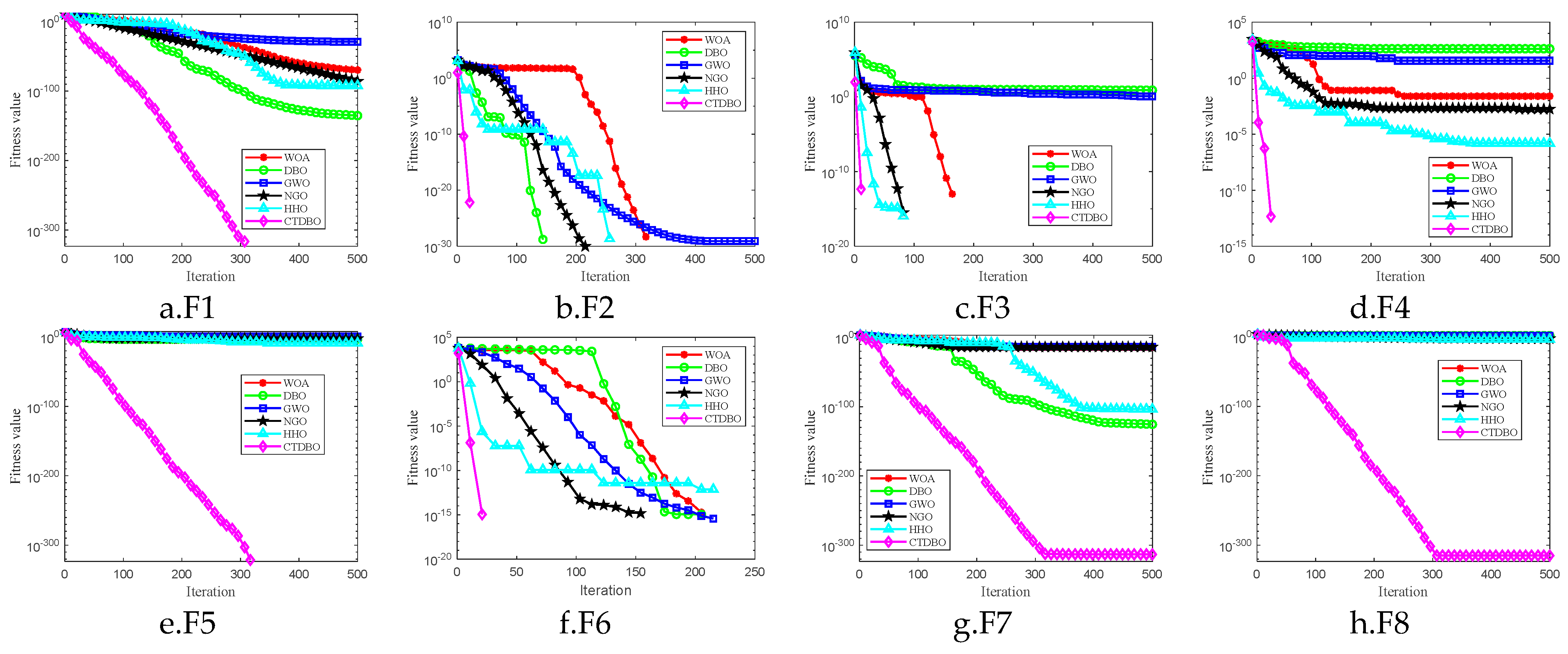
In order to verify the superiority of the CTDBO algorithm proposed in this paper, the Whale Optimization Algorithm (WOA) [31], Grey Wolf Optimization Algorithm (GWO) [32], Northern Goshawk Optimization, (NGO) [33], Harris Hawks Optimization (HHO), [34] and DBO algorithms are used as comparison algorithms. In order to ensure fairness, the population size of all 6 algorithms is set to 30, the maximum number of iterations is 500, the number of runs is 30, and the function dimensionality is 20. A total of 30 times of average (Ave) and standard deviation (Std) are used as the resulting judgement index. In order to reduce the influence of randomness on the results, the Ave is selected as the main index, and the optimal values are highlighted in bold. According to Table 2, the CTDBO algorithm proposed in this paper finds the optimal values for the F1, F2, F3, F6, F7, and F8 test functions. Although the algorithm does not find the optimal values for the F4 and F5 test functions, its optimization results are still more accurate than those of the other five algorithms. To clearly exhibit the effectiveness of the CTDBO compared to other algorithms, Figure 1 presents the convergence curves of these 6 algorithms in 20 dimensions. From the figure, it can be seen that the CTDBO algorithm exhibits the fastest convergence speed, especially when running the F7 and F8 functions, where the optimal value is found after only about 300 iterations.
Table 2.
Algorithm run result.
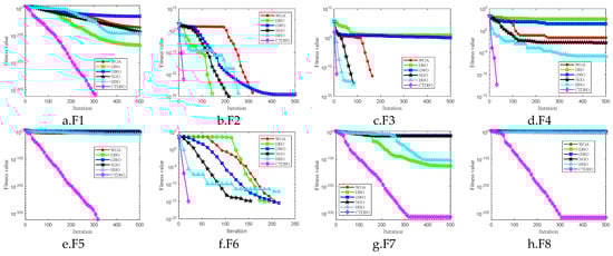
Figure 1.
Test function curve.
In summary, the CTDBO ranks first in both Ave and Std values among the eight groups of test functions and has the fastest convergence speed, which proves that the improvement strategy described in this paper is effective and has superior global search capabilities, and the ability to escape local optima, but also shows fast convergence and good stability.
2.5. Variational Mode Decomposition Algorithm
The variational mode decomposition (VMD) is proposed as an improvement over empirical mode decomposition (EMD), offering an adaptive method for separating signals based on their inherent characteristics. The separation process requires multiple iterations, and since there is no uniform standard to stop the iteration, the IMFs obtained each time can vary. The VMD iteratively seeks the optimal solution of the fitness function to determine the center frequency and bandwidth of each component, which is then used to adaptively separate the signal. This approach effectively suppresses the mode mixing phenomenon of EMD.
The essence of the VMD is to solve a variational problem, whose constraint model is shown in Equation (16). By using Equation (16) as a constraint for VMD, the sequence can be decomposed into modal components with finite bandwidths centered around specific frequencies. This ensures that the sum of the bandwidths of all modes is minimized while the sum of all modes equals the original signal. The solution process is shown in reference [35].
In the equations, is the partial derivative operator. is the Dirac delta function. and are the set of modes and the set of center rates, respectively.
2.6. CTDBO-VMD Model Process
The number of decomposition layers and the penalty factor of the variational modal decomposition are two parameters that play a key role in the accuracy of the decomposition; it is difficult to set these parameters accurately based on empirical methods due to the stochastic and intermittent nature of power loads. If the value is large, the algorithm will over-decompose and produce false components; on the contrary, it will lead to insufficient decomposition and affect the final prediction accuracy. At present, there is no exact method to confirm the value of the , most of them are set empirically, and then an approximate value is determined through continuous adjustment, but this method cannot determine whether the penalty factor is optimal or not, and if it is too large, it will result in the loss of band information; on the contrary, it will lead to information redundancy.
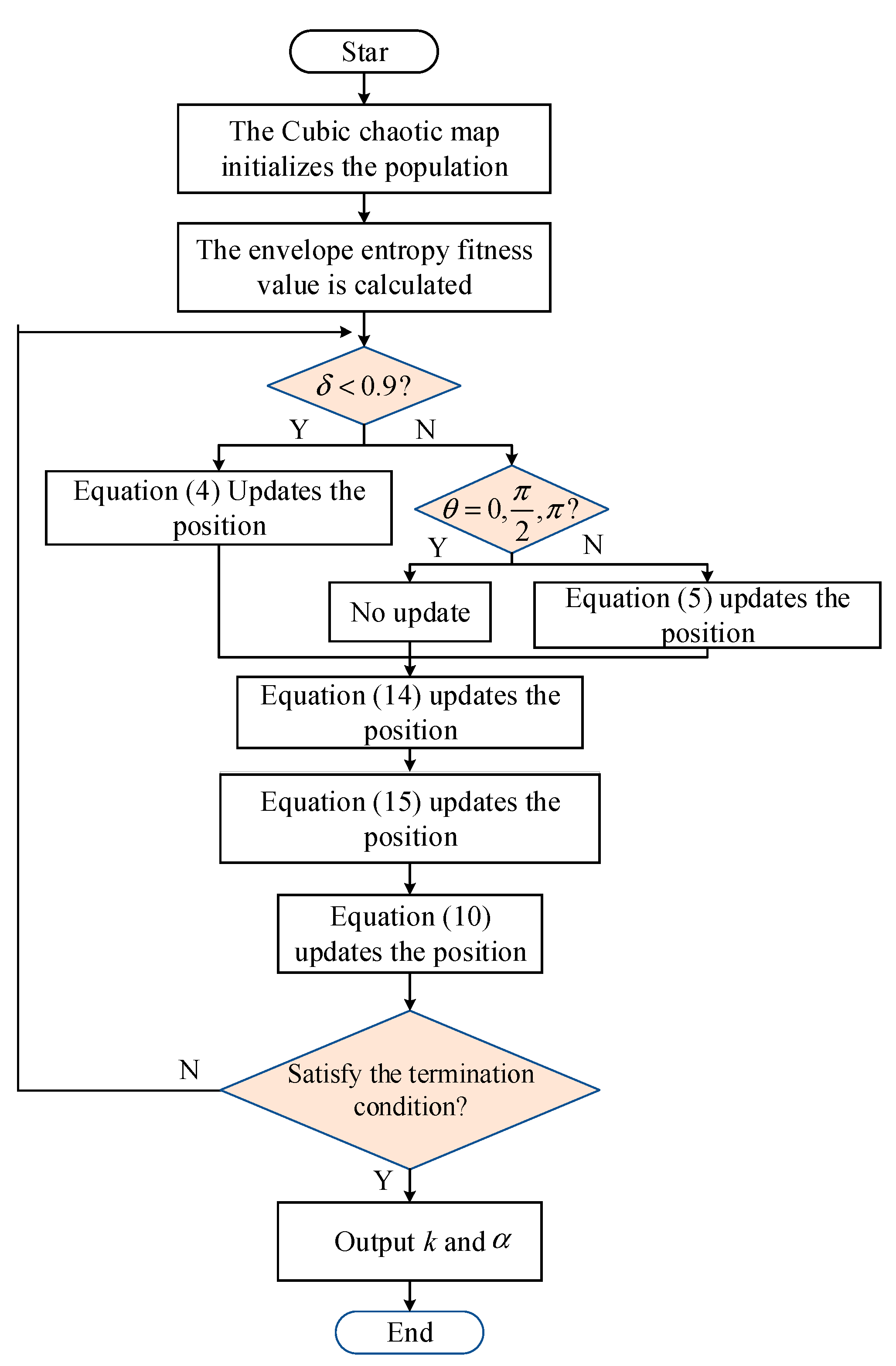
The CTDBO algorithm for of the optimization process is used in the process of solving the fitness function; this paper selects the envelope entropy as the fitness function of the VMD, through the CTDBO algorithm iterating continuously to obtain the minimum solution that is the optimal solution of . The formula of envelope entropy is shown in equation (17), and the flow of the CTDBO-VMD is shown in Figure 2.
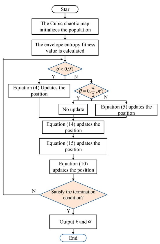
Figure 2.
Flow chart of CTDBO-VMD model.
In the equations, is the envelope signal. is the normalized expression of the envelope signal.
3. Combined Forecasting Model
3.1. Convolutional Neural Networks
Convolutional neural networks are popular among scholars for their high efficiency, adaptability, and robustness [36]. A CNN has input, convolutional, pooling, and fully connected and output layers, the core of which is the convolutional layer, which mainly performs feature extraction tasks. In this paper, we chose to add convolutional layers and pooling layers to extract the period and trend of the load sequence so as to improve the prediction accuracy of the model. The formula for the convolutional layer is as follows:
In the equations, is the input to the convolution kernel. is the activation function. is the set of input mapping layers. is the weight matrix of the convolution kernel. is the bias term.
3.2. Bidirectional Long- and Short-Term Memory Networks
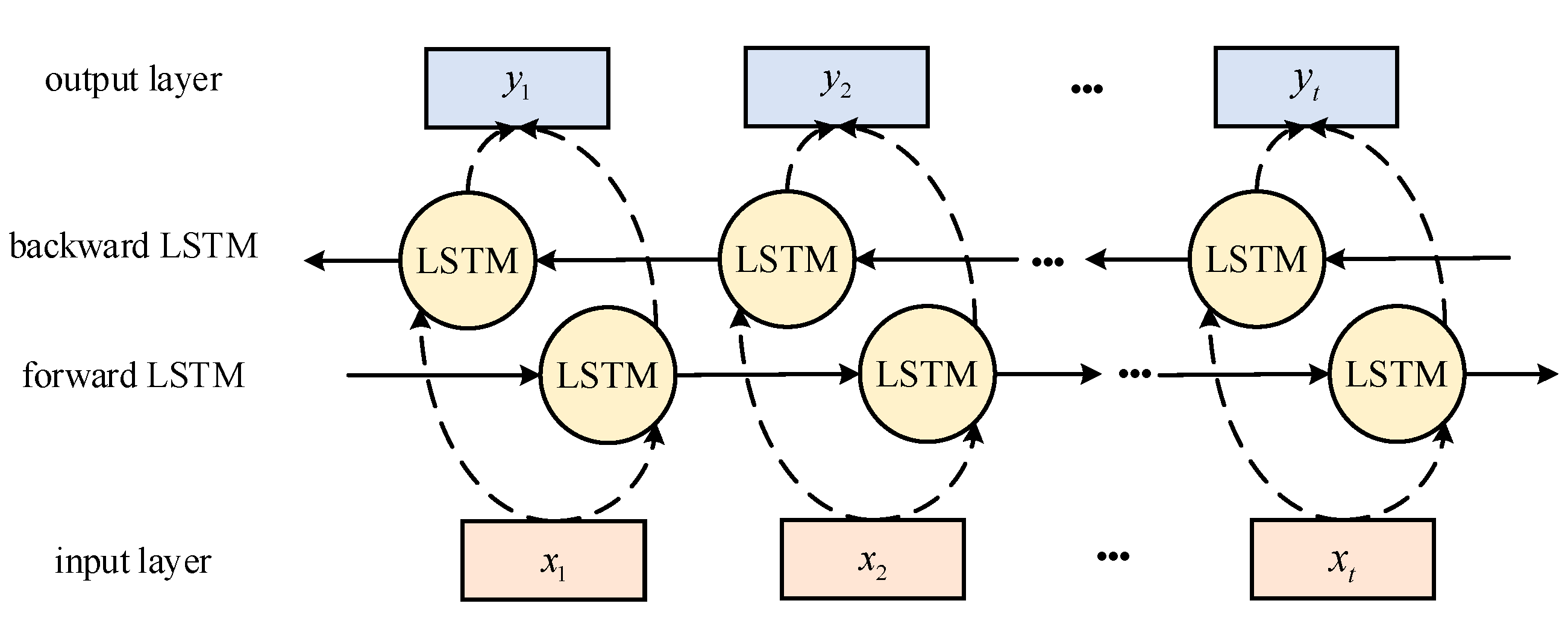
LSTM adds gating units to RNN, which can adaptively retain or forget information, and therefore has better performance when processing large amounts of data [37]. BILSTM is an extension of LSTM, which combines two LSTM layers; one processes input sequences from start to finish, while the other processes them from end to start. Compared to LSTM, BILSTM improves model stability and reduces the possibility of gradient vanishing and gradient explosion by allowing gradients to propagate in both directions when processing data in both directions. The structure of BILSTM is shown in Figure 3.

Figure 3.
BILSTM structure diagram.
For the BILSTM, the hidden layer states
In the equations, is the forward LSTM hidden layer state at moment t. is the backward LSTM hidden layer state at moment t. is the output at moment t. is the input at moment t. is the weight matrix. is the paranoia item.
3.3. Attention Mechanism
The AM is a technique inspired by human visual attention and has been proposed for use in deep learning [38]. In this paper, the AM is combined with the CNN-BILSTM. Firstly, a CNN extracts local features from the load sequence, allowing the model to better learn short-term trends and periodic patterns. Then, the features extracted by a CNN are fed into the BILSTM to further extract the temporal patterns of the load sequence over a long span of time. Finally, the AM is added to dynamically assess the importance of different features and assign appropriate weights to them. The most critical part of the AM is the scoring function, which determines the importance of each feature. The formula is as follows:
In the equations, is the weight. is the deviation. tanh is the activation function.
The weights of different vectors are obtained by normalizing them using the Softmax function
In the equations, is the attention value; is the AM layer output at moment t.
3.4. Two-Wash and CTDBO-VMD-CNN-BILSTM-Attention Prediction Models
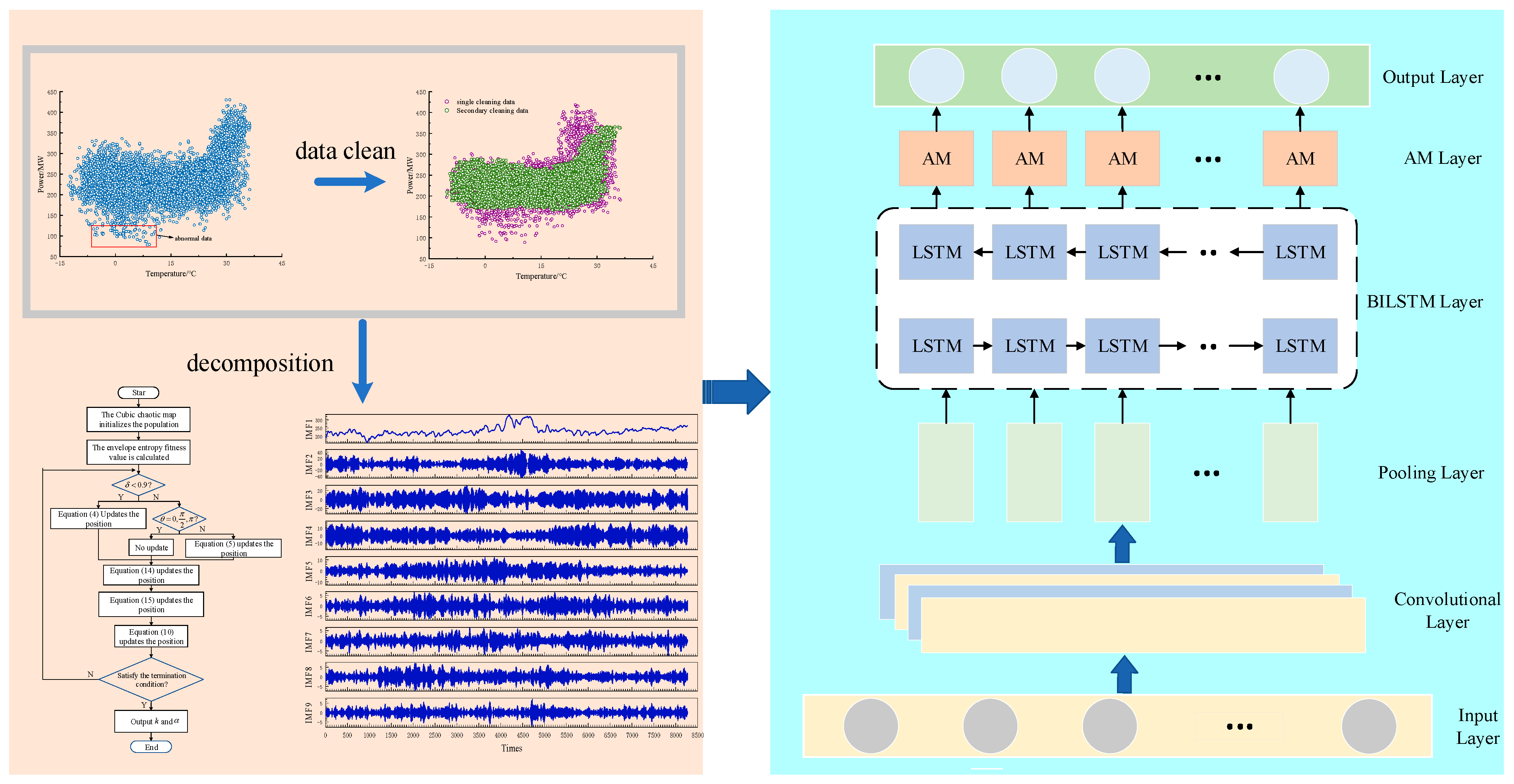
Nowadays, power loads are generally recorded by devices such as smart meters. Although these devices have high stability and reliability, they may still encounter problems, such as abnormal data transmission or large errors in power metering due to lack of regular maintenance. As a result, the collected load sequence data may contain outliers and nulls. In this paper, we use neighborhood averages to fill in the nulls, followed by the K-means and the DBSCAN for secondary cleaning to eliminate outliers. Then, the CTDBO algorithm is applied to optimize the parameters of and of the VMD, with the optimal values used to decompose the load sequence into multiple IMFs with different frequencies. These IMFs are input into the convolutional and pooling layer of the CNN to extract important features, reducing input redundancy and the dimensionality of the data. The important features are fed into the BILSTM layer to capture the long-term temporal relationships. Finally, the attention mechanism (AM) assigns different weights to key time periods or data points, enhancing the model’s focus on critical information and thereby improving prediction accuracy. The secondary cleaning and the CTDBO-VMD-CNN-BILSTM-AM prediction model is illustrated in Figure 4.
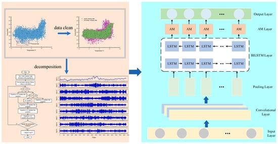
Figure 4.
Secondary cleaning and CTDBO-VMD-CNN-BILSTM-Attention prediction models.
3.5. Indicators for Model Evaluation
In order to evaluate the model objectively, the root mean square error (RMSE), mean absolute percentage error (MAPE), relative analysis error (RPD), and mean absolute error (MAE) are chosen as the evaluation metrics in this paper. The RMSE indicates the average deviation of the prediction from the target. The MAPE is used to assess the accuracy of prediction model. The RPD measures the model’s fit, a larger RPD value indicates higher prediction accuracy [39,40]. The MAE reflects the degree of deviation between the predicted value and the target; a smaller MAE value indicates higher model accuracy.
In the equations, is the sample size. indicates the predicted value. indicates target value. indicates the average of the target values.
4. Data Processing
In this paper, the annual power load data from 1 January to 31 December 2018 in a region of Inner Mongolia are selected as the dataset, with a sampling interval of 1 h, resulting in a total of 8760 data points. The data include the six characteristic variables of humidity, temperature, wind speed, pressure, visibility, and water vapor pressure, as well as the actual power load value.
Since the presence of missing values in the dataset may cause the model to fail in accurately capturing the patterns and trends in the load series, and since there is a correlation between the missing values and the preceding and following data, this paper uses the squared mean method to fill in the gaps. Assuming there are missing values at a certain point, the calculation is as follows:
4.1. Feature Variable Selection
Since the dataset contains six feature variables, to minimize the mutual influence between these variables and reduce data redundancy, both of which can lower the model’s prediction accuracy, this paper uses Pearson correlation coefficients to calculate the correlation between different characteristic variables and electricity load, and selects the strong correlation variables as inputs to the model. The correlation coefficients are shown in Table 3. From Table 3, it can be seen that temperature has strong correlation with electricity load, and the rest of the characteristic variables are moderately correlated and weakly correlated with electricity load, so this paper selects temperature as the input of the model.
Table 3.
Characteristic variable and load Pearson correlation coefficient.
4.2. K-means Algorithm for One Cleaning
Since the range of values of the power load is much larger than that of the temperature, and also to improve the identification and processing of outliers, the data need to be normalized [41]. The formula is as follows:
In the equations, represents the normalized data. are the raw data. indicates the minimum value of the data. indicates the maximum value of the data.
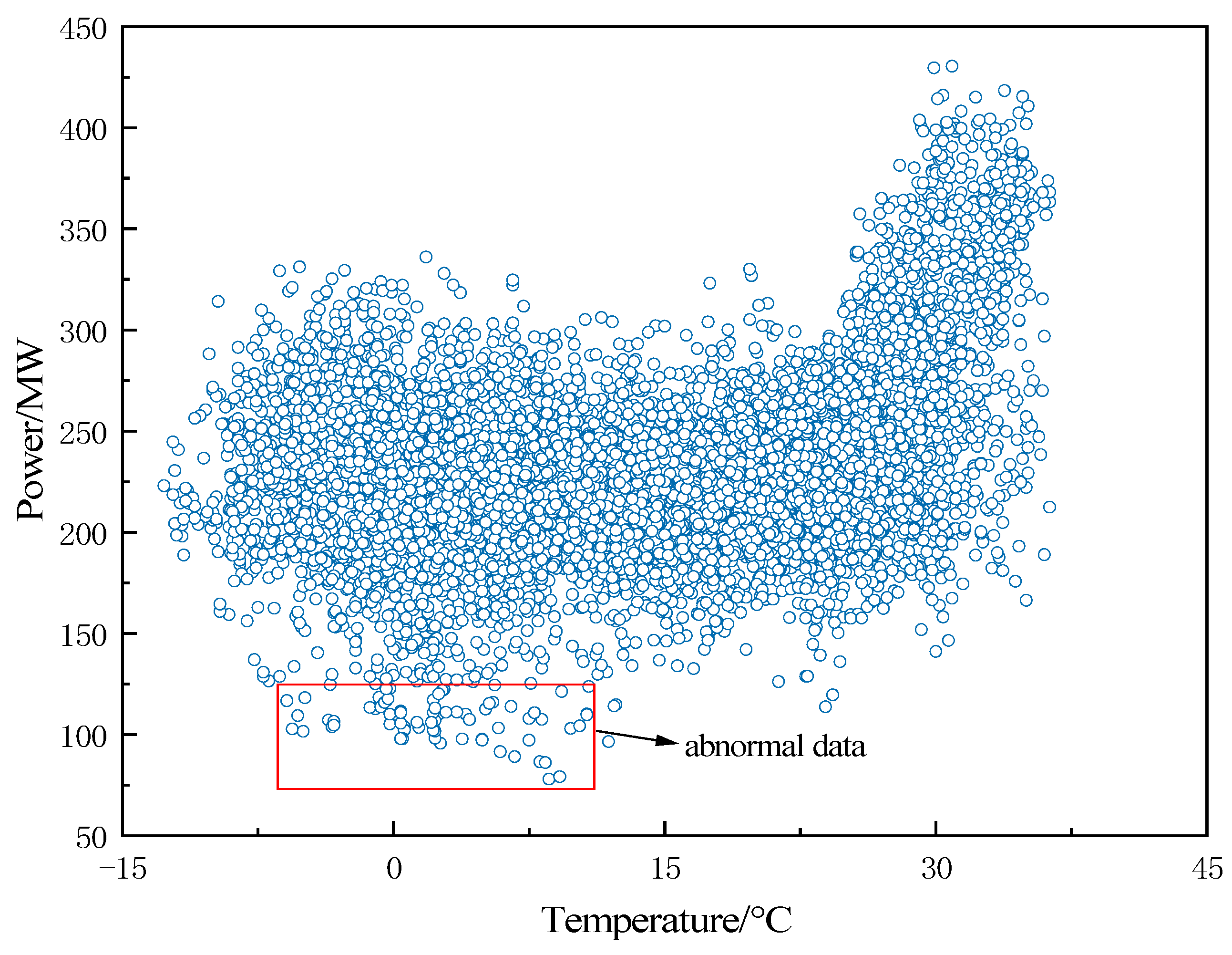
The normalized raw load series is shown in Figure 5, which contains a large number of scattered points, which may be outlier data due to recording errors or special festivals and unusual events and are therefore collectively classified as outliers.
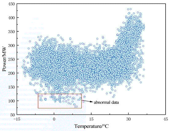
Figure 5.
Scatter plot of original load sequence.
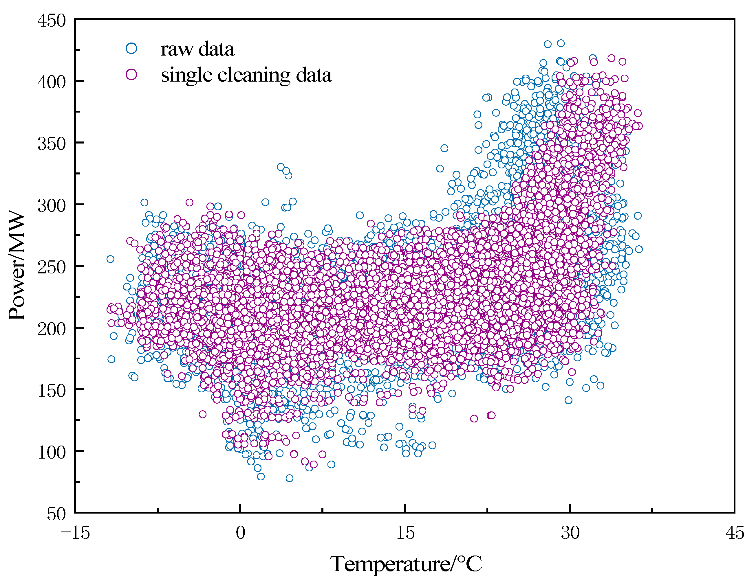
In this paper, a week is used as the prediction time span. The K-means algorithm is applied to divide the data of 365 days of the year into 52 clusters, and each cluster contains a total of 168 data points for 7 days. In this paper, a threshold value is added to the K-means algorithm. This threshold is set at the 95th percentile of the Euclidean distance from the closest point to the center of each cluster. If the Euclidean distance from a data point to the cluster center exceeds this threshold, the point is considered an anomaly and is excluded. The cleaning result is shown in Figure 6. From the figure, it can be seen that the outliers are obviously reduced, and the data with load values in the range of 300 MW to 400 MW have become more compact. After cleaning with the K-means algorithm, 8586 data points remain, effectively eliminating 174 anomalies. However, there are still fewer abnormal data, so further decomposition of the data is necessary.

Figure 6.
K-means data cleaning result.
4.3. DBSCAN Secondary Cleaning
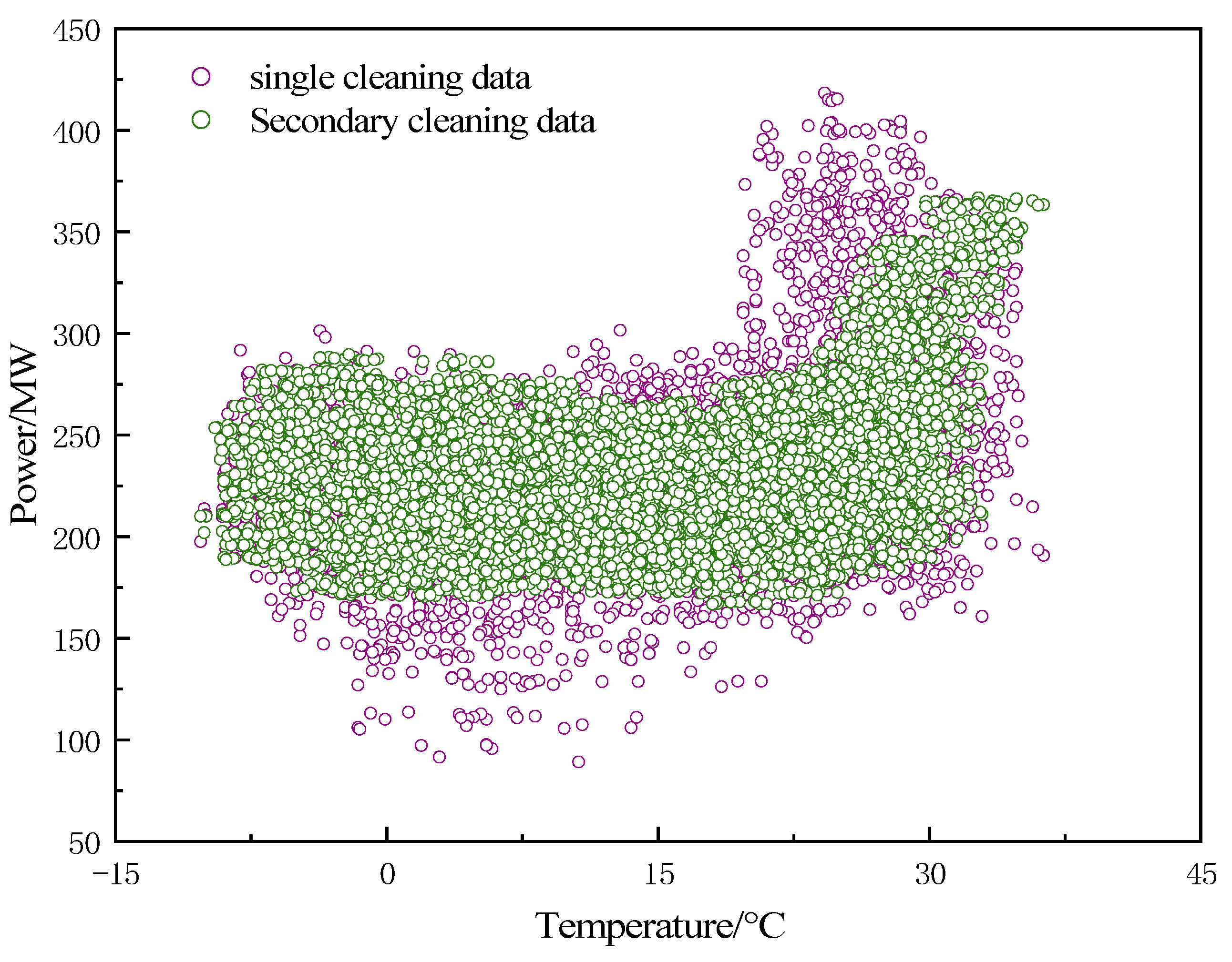
Since the K-means algorithm fails to remove all the anomalies, there are still a few anomalies and noise in the load sequence, Therefore, this paper adopts the DBSCAN algorithm for secondary cleaning. The DBSCAN algorithm is mainly based on the core points of the data to be clustered, so the number of core points significantly affects the quality of the clustering results. After continuous attempts to set MINPts to 10 and to 2 its data cleaning results are optimal, and the secondary cleaning results are shown in Figure 7. According to the result graph, it can be seen that the remaining low-density clusters are eliminated after the primary cleaning, which makes the data clusters tighter and more evenly distributed, so the parameters of the DBSCAN algorithm are set appropriately, and the cleaned data no longer contain outliers and noise.
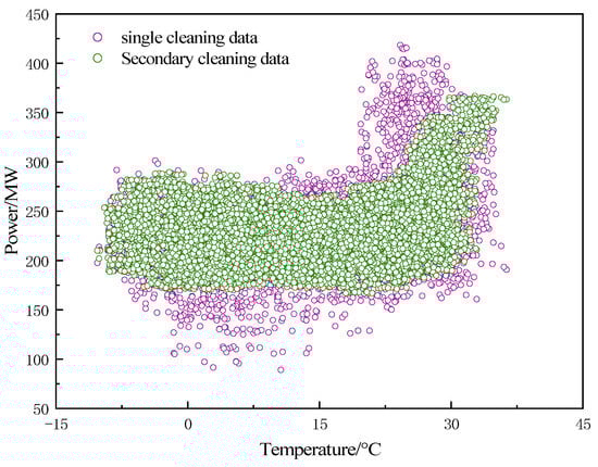
Figure 7.
DBSCAN indicates the result of secondary cleaning.
Outliers can impact the accuracy of prediction models, leading to a reduced generalization ability. By cleaning the data using clustering algorithms, the interference of outliers and noise in model training can be minimized, thereby improving the accuracy of the prediction models. K-means clustering aids in detecting outliers by assigning data points to K cluster centers and identifying those that are far from these centers, which are often outliers. The DBSCAN, on the other hand, identifies points in low-density regions, which may also be outliers, based on the concept of density. These two methods enable the rapid detection and removal of outliers from the dataset, saving time compared to manual outlier removal.
5. Experimental Results and Analysis
5.1. VMD Decomposition Results
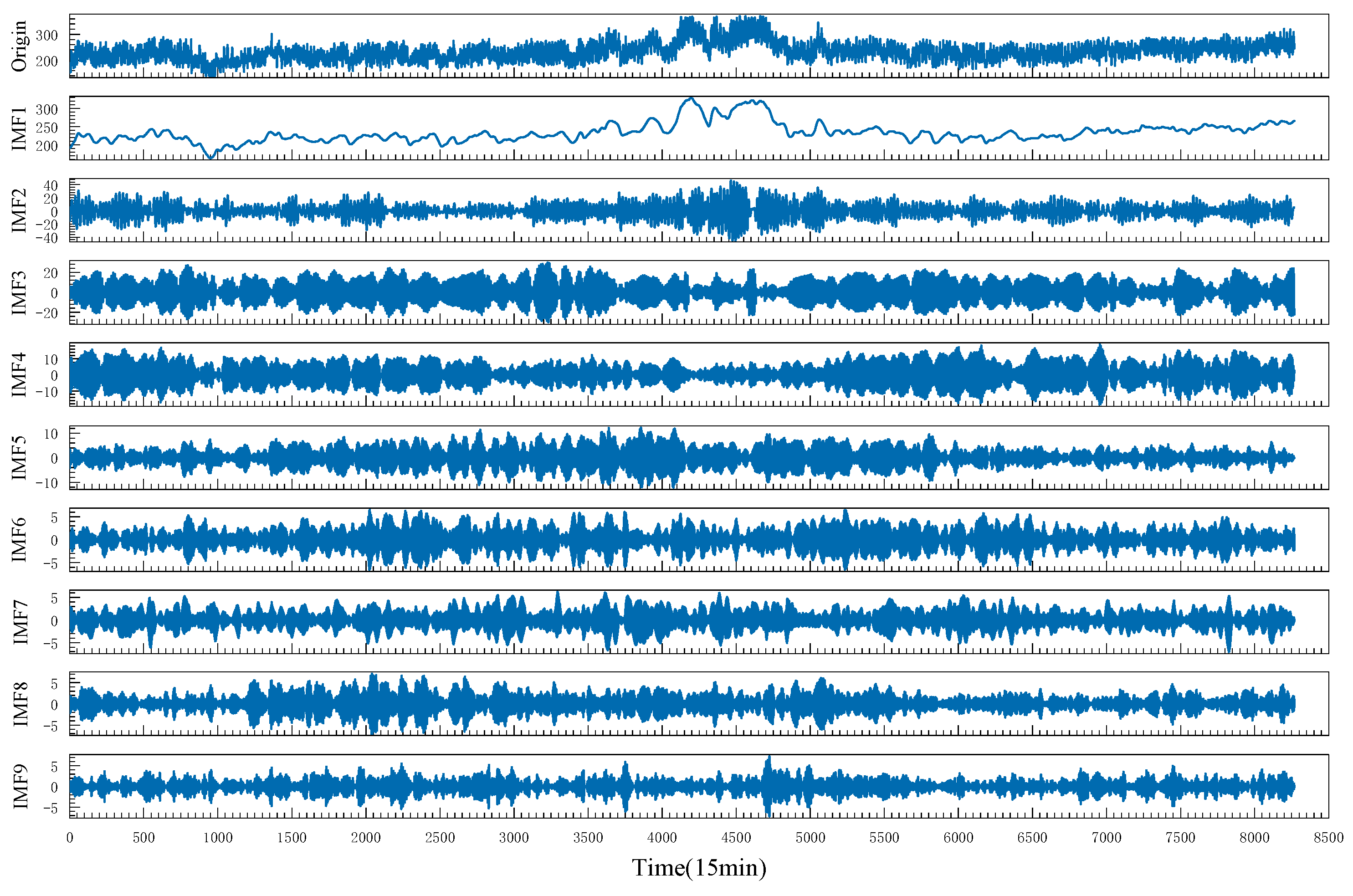
In order to reduce the VMD decomposition tuning time and make the decomposition results more accurate, this paper uses the CTDBO algorithm to optimize the parameters and of the VMD. The population size in the CTDBO algorithm is set to 20, and the number of iterations is set to 15. The upper bound of optimization of the VMD is , and the lower bound of optimization is . The final optimization search result is , and the result is shown in Figure 8. From the analysis of Figure 8, it can be seen that the VMD algorithm decomposes the load sequence into nine IMFs with frequencies ranging from high to low. Observing the waveform of each IMF, all show symmetry and clear frequency separation, so that the load sequence is completely decomposed when .
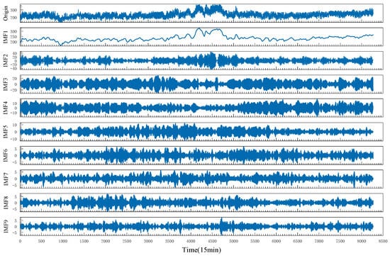
Figure 8.
VMD decomposition result.
5.2. Single Model Predictions
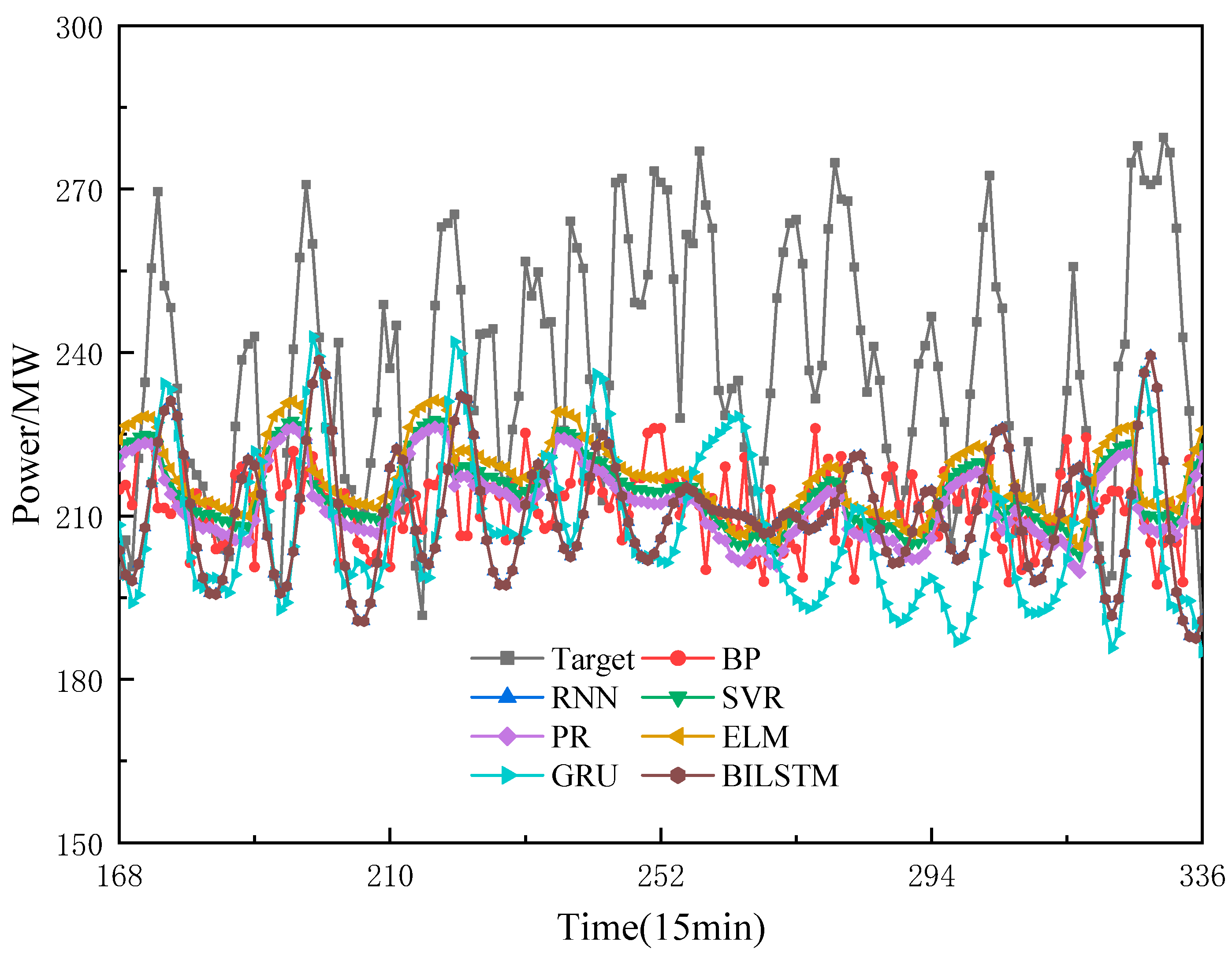
In order to verify the effectiveness and prediction accuracy of BILSTM, the BP neural network, extreme learning machine (ELM), support vector regression (SVR), polynomial regression (PR), gated recurrent unit (GRU) and RNN are selected as comparison models in this paper. The training set kernel test set is divided according to the ratio of 8:2. Among them, the number of neurons in the hidden layer of BP neural network is 200, and the maximum number of iterations is 500. The number of neurons in the hidden layer of ELM is 200. The linear kernel function is selected for SVR. PR uses a first-order polynomial. The number of neurons in the hidden layer, the maximum number of iterations, and the learning rate of GRU, RNN, and BILSTM are , and the rest of the parameters are default values. To ensure fairness, all experiments use the power load sequence after secondary cleaning as the dataset. The experimental software is MATLAB 2021a. For easier observation, the load of the second week of 2018 is used as the prediction target. The prediction results are shown in Figure 9, and the model evaluation indices are presented in Table 4. According to Figure 9, it can be seen that the prediction accuracy of single models is not high, especially the prediction curve trends of ELM, PR, and SVR, which show significant differences in similarity with the target, and the fit is poor. This proves that it is difficult for a single machine learning model to make effective prediction of complex power loads. The BP neural network has the worst prediction accuracy among the deep learning networks. The prediction curve trend in the early stage of GUR is similar to that of the target, and it is distorted from the 238th node onwards. Trough prediction accuracy is greatly reduced, which may be due to gradient disappearance or overfitting phenomenon. Compared with GRU, the curve trend of BILSTM in the early stage is close to and more similar to the target, but in the later stage, BILSTM’s fit is better than that of GRU’s, as can be seen from Table 4. Compared with GRU, the RMSE, MAE, and MAPE of BILSTM decreased by 4.817 MW, 2.393 MW and 1.873 percentage points, respectively. Moreover, the RPD index of BILSTM improved by 0.15 compared with GRU, and since the larger the RPD the higher the model accuracy, the prediction accuracy and stability of BILSTM are better than GRU.

Figure 9.
Single model prediction results.
Table 4.
Evaluation index of a single model.
In summary, the prediction accuracy, curve trend, and stability of BILSTM are better than the other five groups of models.
5.3. Comparison of Ablation Experiments
In order to verify the effectiveness and accuracy of the CTDBO-VMD-CNN-BILSTM-Attention (model 1) proposed in this paper, the VMD-BILSTM (model 2), CTDBO-VMD-BILSTM (model 3), CNN-BILSTM-Attention (model 4), and VMD-CNN- BILSTM-Attention (model 5) are used as comparisons. The parameter settings for the CTDBO algorithm were the same as those in Section 4.1, and the VMD parameters for model 2 and model 5 were set manually with values of . The predicted results of the ablation experiment are shown in Figure 10, and the model evaluation metrics are shown in Table 5.
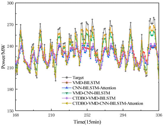
Figure 10.
Ablation results.
Table 5.
Evaluation index of ablation experiment.
The prediction results demonstrated that the prediction accuracy of the combined model is higher than that of the single model. The results of the VMD-BILSTM are better than that of the single BILSTM, with the RMSE, MAE, and MAPE reduced by 18.082 MW, 16.861 MW, and 6.731 percentage points, respectively, RPD has improved by 0.441, demonstrating that the VMD can extract the key features in the load sequence. This proves that the VMD can extract the key features in the load sequence and reduce the data dimension, which effectively improves the prediction accuracy of the complex data. The CTDBO-VMD-BILSTM show significant improvement in the performance of both the curve trend and the goodness-of-fit compared to the VMD-BILSTM. This important aspect is attributed to the fact that the CTDBO algorithm can accurately find the optimal parameter combinations of the VMD, which makes the decomposition of the load sequence more thorough, and thus improves the performance and prediction accuracy of the model. The prediction results of the VMD-CNN-BILSTM are better than those of the VMD-BILSTM, CNN-BILSTM-Attention and CTDBO-VMD-BILSTM, which proves that the VMD decomposes the load sequence into IMFs with different frequencies. The convolutional and pooling layers of the CNN extract the important features of the IMFs, improving the model’s prediction ability. The CTDBO algorithm can find the best combination of parameters of the VMD, which makes the load sequence decompose more thoroughly, thus improving the performance and prediction accuracy of the model. The CTDBO-VMD-CNN-BILSTM-Attention model’s curve trend is most similar to the target, maintaining high prediction accuracy in both peaks and valleys. Compared to the VMD-CNN-BILSTM model, the RMSE, MAE and MAPE are reduced by 5.377 MW, 2.098 MW and 2.003 percentage points. in addition, the model proposed in this paper has an RPD greater than 3, which proves that the model has high prediction accuracy, stability, and robustness.
5.4. Comparison of Different Models
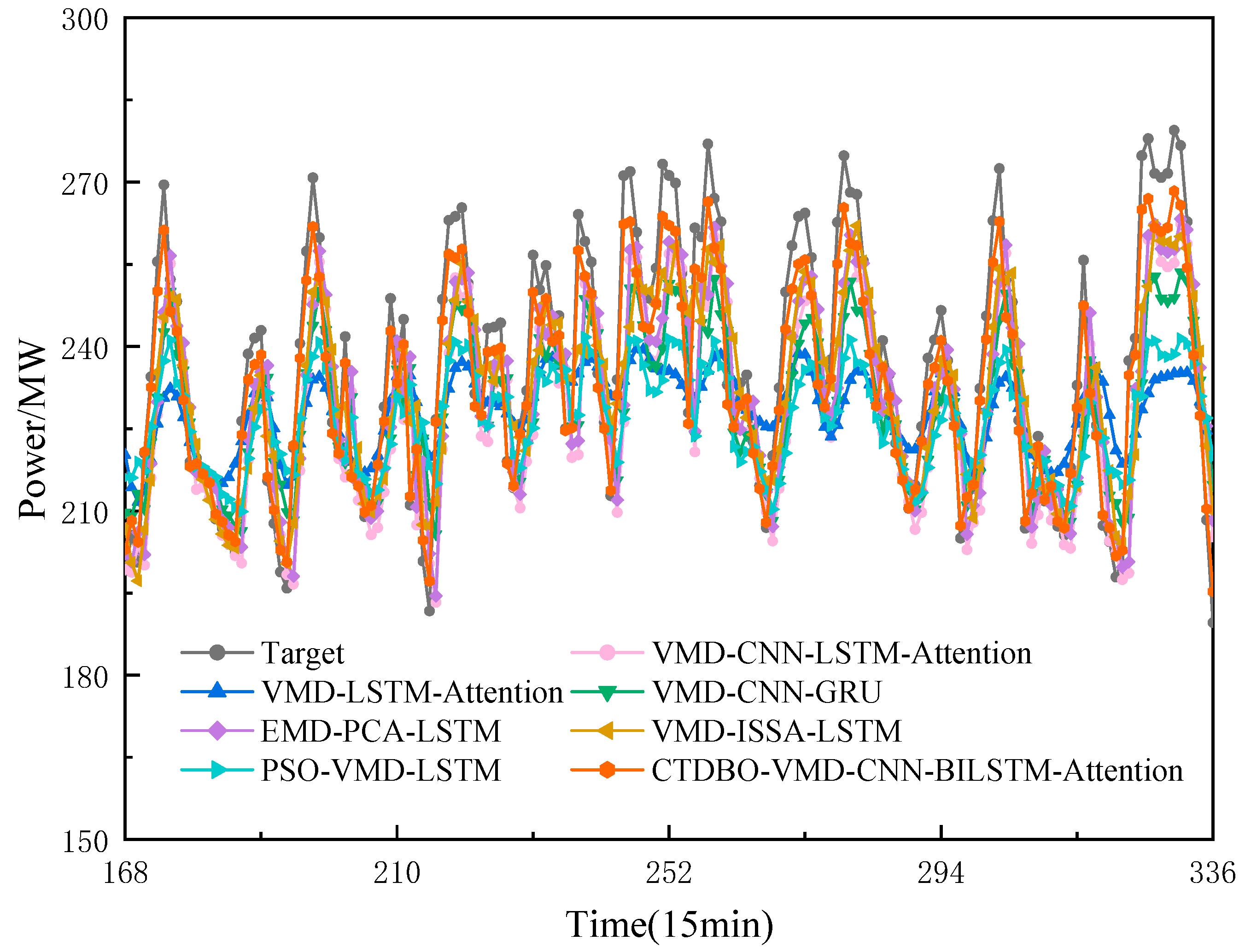
In order to verify the superiority of the models proposed in this paper, the VMD-CNN-GRU [42] (model 6), VMD-CNN-LSTM-Attention [43] (model 7), VMD-ISSA-LSTM [44] (model 8), EMD-PCA-LSTM [45] (model 9), VMD-LSTM-Attention [46] (model 10), PSO-VMD-LSTM [47] (model 11) were used as comparison models. The VMD parameters of model 6, model 7, model 8 and model 10 are set to . The number of neurons in the hidden layer, the maximum number of iterations and the learning rate of GRU and LSTM are . The population size of ISSA and PSO is set to 20, the number of iterations is 15, the discovery ratio of SSA is 0.2, the inertia factor of PSO is 0.9, and the maximum velocity of the particles , is the minimum velocity . The rest of the parameters are set to their default values. The results of the intelligent algorithm are shown in Table 6, the model prediction results are shown in Figure 11, the model error is shown in Figure 12, and the model evaluation index is shown in Figure 13.
Table 6.
Intelligent algorithm to optimize results.
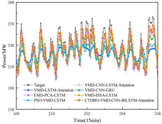
Figure 11.
Comparison of model prediction results.
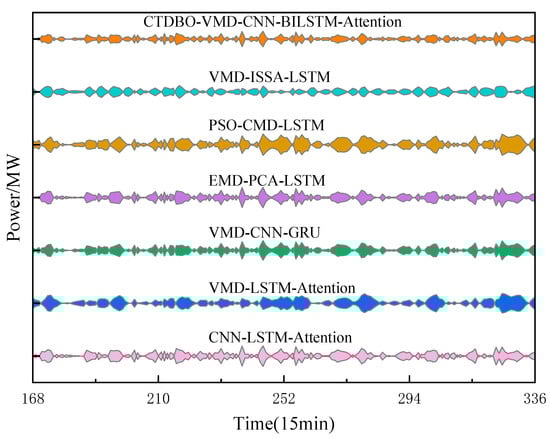
Figure 12.
Model error comparison diagram.
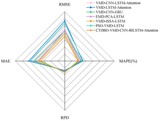
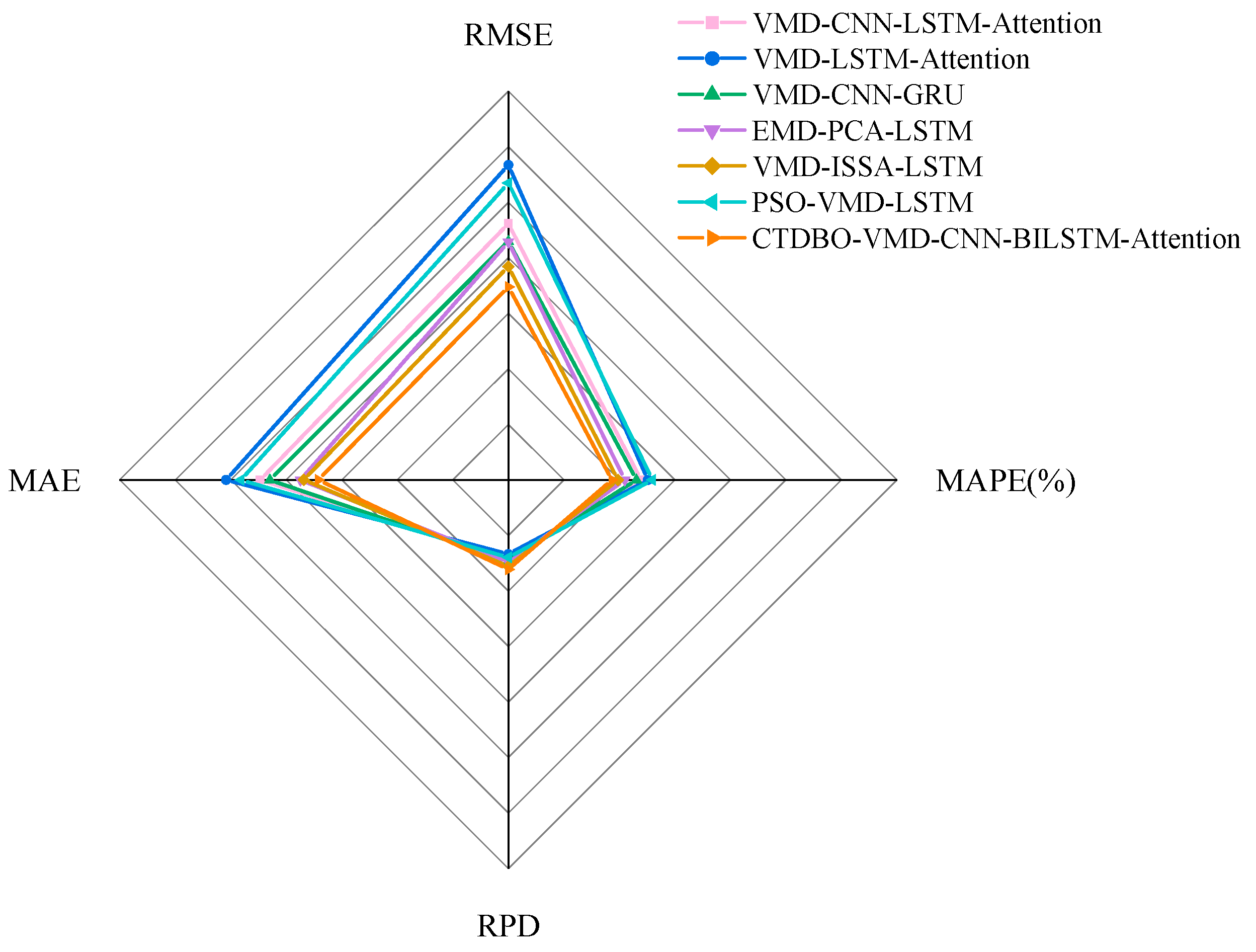
Figure 13.
Model index radar chart.
According to Figure 10, the curve trends and the predicted values of peaks and valleys for the combined PSO-VMD-LSTM and VMD-LSTM-Attention models show a large gap compared to the target. Additionally, Figure 11 shows that the prediction model error kite diagrams for the peaks and valleys of the PSO-VMD-LSTM and VMD-LSTM-Attention in the 210–240 interval are larger than those of the other models, indicating that those two models have larger prediction errors in this interval. The troughs are larger than those of the other models, indicating that the prediction errors of these two models in this interval are larger. In addition, the graph of the model evaluation metrics shows that the RMSE, MAE and MAPE of the evaluation metrics of the PSO-VMD-LSTM and VMD-LSTM-Attention are larger than those of the other models, while the RPD is smaller, indicating that the prediction accuracies of these two models on this dataset are lower, less stable, and less robust. Figure 10 shows that the prediction curves of the VMD-CNN-LSTM-Attention, EMD-PCA-LSTM and VMD-ISSA-LSTM models have similar trends and align closely with the target. Moreover, the prediction errors of these three groups models at the nodes with larger fluctuations or peaks and valleys are significantly smaller than those of the PSO-VDM-LSTM and VMD-LSTM-Attention models. The RMSE, MAE and MAPE of the VMD-ISSA-LSTM model are the smallest, and the RPD is the largest, so that the performance of the VMD-ISSA-LSTM model is ranked the highest among the three groups of models. The GJO-VMD-CNN-BILSTM-Attention proposed in this paper is the most similar to the target both in predicting the curve trend, fit, and peak and trough predictions. It also has the smallest area and narrowest width at nodes with large fluctuations, such as peaks and troughs, which proves that the difference between the predicted values of the model proposed in this paper and the target is the smallest. Additionally, the model has the lowest RMSE, MAE, and MAPE and the RPD is large compared to the VMD-ISSA-LSTM, making the accuracy of the model proposed in this paper better than that of the VMD-ISSA-LSTM.
In summary, the CTDBO-VMD-CNN-BILSTM-Attention model has high prediction accuracy, robustness, and stability.
6. Discussion
The CTDBO-VMD-CNN-BILSTM-AM hybrid forecasting model proposed in this paper demonstrates superior performance in power load forecasting, outperforming traditional models and other hybrid models across multiple evaluation metrics. Compared to the DBO algorithm, the CTDBO algorithm offers faster optimization speed and higher precision, enabling rapid identification of the optimal parameter combination for the VMD algorithm and saving a substantial amount of time that would otherwise be spent on manual parameter tuning. The CNN-BILSTM-Attention hybrid model incorporates steps for feature extraction, temporal dependency handling, and the use of the attention mechanism to enhance the model’s sensitivity to critical data. This approach effectively analyzes and forecasts the IMFs obtained from the VMD decomposition, thereby improving the accuracy and reliability of power load forecasting. Although the model proposed in this paper exhibits strong performance, it still has certain limitations:
- Performing Pearson correlation analysis on the feature variables influencing power load can reduce feature redundancy and improve model prediction accuracy. However, these correlations may be affected by regional variations, which can impact the model’s accuracy.
- While hybrid forecasting models offer better prediction accuracy and stability compared to simpler models, they also increase the prediction time.
- This study only considers short-term power load forecasting. Future work could extend to medium-term and long-term load forecasting. This would facilitate a more comprehensive assessment of changes in power demand trends, support longer-term electricity planning and decision-making, and enhance the overall operational efficiency of the power system.
7. Conclusions
To address the difficult prediction problem caused by the nonlinearity and high volatility of power load, this paper firstly uses the K-means and DBSCAN algorithms to carry out secondary data cleaning of the original load sequence to eliminate outliers. Then, the CTDBO algorithm seeks the optimality of the number of decomposition layers and the penalty factor of the VMD to decompose the cleaned power load sequence into several IMFs with different frequencies. Finally, the IMFs are input into the CNN-BILSTM-Attention model for feature extraction and prediction, and the following conclusions are drawn by comparing with different models:
- (1)
- Most of the anomalies in the original power load sequence can be eliminated after K-means primary cleaning, but there is still a small number of anomalies or noise. The secondary cleaning of the primary cleaned data using the DBSCAN density clustering algorithm can effectively remove the residual anomalies and noise, improve the purity and quality of the data, and make the subsequent analysis and modeling more reliable and accurate.
- (2)
- By using the envelope entropy as the fitness function, the CTDBO algorithm is used to optimize the number of decomposition layers and penalty factors of the VMD algorithm, ensuring that the optimal number of decomposition layers and penalty factors is obtained. This strengthens the applicability of the VMD, effectively reduces the randomness of the VMD parameters and the time required for parameter tuning, and improves the stability and accuracy of the decomposition results.
- (3)
- The IMF obtained from the VMD decomposition is input into the CNN, where deep feature extraction and learning are performed through convolutional and pooling layers to obtain important information from complex signals. Then, the extracted information is input into the BILSTM to process from forward and backward logarithms and different weights are given to different features through the attention mechanism. The effectiveness of the CTDBO-VMD-CNN-BILSTM-Attention model proposed in this paper is demonstrated through experiments and showing higher prediction accuracy and superiority compared to other models.
- (4)
- Through validation with the Inner Mongolia power load dataset, the proposed model demonstrates good accuracy and stability. It is capable of handling complex data patterns and fluctuations commonly encountered in power load forecasting. By using the model’s prediction results as a reference, grid operators can more effectively balance power supply and demand, thereby reducing scheduling errors. The proposed power load forecasting model primarily provides reliable load prediction data for grid operators, electricity trading markets, and policymakers. This enhances the stability of the power system, optimizes electricity market trading strategies, and supports the formulation of informed energy policies. Furthermore, the prediction results of this model can provide valuable references for integrating renewable energy sources such as wind and solar power into the grid, thereby improving the stability and efficiency of the power system.
Author Contributions
Conceptualization, D.W. and S.L.; data curation, D.W. and S.L.; methodology, D.W. and X.F.; software, D.W. and S.L.; formal analysis, D.W., S.L. and X.F.; writing and original draft preparation, D.W. and S.L.; review and editing, D.W., S.L. and X.F. All authors have read and agreed to the published version of the manuscript.
Funding
This work was financially supported by the National Natural Science Foundation of China [grant number 11202078]; Educational Commission of Shanghai of China [grant number 13ZZ145]; Natural Sciences Foundation of Shanghai Committee of Science and Technology [grant number 11ZR1413800]; Foundation of Shanghai Dianji University [grant number 10C102].
Data Availability Statement
Data are contained within the article.
Conflicts of Interest
The authors declare no conflicts of interest.
References
- Yang, S.; Zhou, Z.; Chen, Y.; Liu, J.; Gong, Y. Short-term power load forecasting method considering regional adjacency characteristics. J. Power Syst. Its Autom. 2024, 1–10. [Google Scholar] [CrossRef]
- Wang, C.; Wang, R.; Yu, H.; Song, Y.; Yu, L. Coordinated planning problems and challenges under the evolution of distribution network morphology. Chin. J. Electr. Eng. 2020, 40, 2385–2396. [Google Scholar]
- Sun, D.; Zhao, L.; Sun, K.; Wang, Y.; Sun, Y. Research on location and capacity optimization strategy of hybrid energy storage in distribution system with new energy access. J. Sol. Energy 2024, 45, 423–432. [Google Scholar]
- He, X.; Zhao, W.; Gao, Z.; Zhang, Q.; Wang, W. A hybrid prediction interval model for short-term electric load forecast using Holt-Winters and Gate Recurrent Unit. Sustain. Energy Grids Netw. 2024, 38, 101343. [Google Scholar] [CrossRef]
- Sun, X.; Bao, M.; Ding, Y.; Xu, H.; Song, Y.; Zheng, C.; Gao, X. Modeling and evaluation of probabilistic carbon emission flow for power systems considering load and renewable energy uncertainties. Energy 2024, 296, 130768. [Google Scholar] [CrossRef]
- Fang, N.; Chen, H.; Deng, X.; Xiao, W. Short-term power load forecasting based on VMD-ARIMA-DBN. J. Power Syst. Autom. 2023, 35, 59–65. [Google Scholar]
- Tang, T.; Jiang, W.; Zhang, H.; Nie, J.; Xiong, Z.; Wu, X.; Feng, W. GM (1,1) based improved seasonal index model for monthly electricity consumption forecasting. Energy 2022, 252, 124041. [Google Scholar] [CrossRef]
- Nie, H.; Wang, F.; Zhao, Y. Power Load Prediction Based on Multiple Linear Regression Model. J. Residuals Sci. Technol. 2016, 13. [Google Scholar]
- Yang, G.; Zheng, H.; Zhang, H.; Jia, R. Short-term load forecasting based on Holt-Winters exponential smoothing and time convolution network. Power Syst. Autom. 2022, 46, 73–82. [Google Scholar]
- Zhang, J.; Wang, S.; Tan, Z.; Sun, A. An improved hybrid model for short term power load prediction. Energy 2023, 268, 126561. [Google Scholar] [CrossRef]
- Rong, G.; Arnaldo, M.; Elie, B.; Zhao, B.; Mohamad, S. Artificial Intelligence in Healthcare-Review and Predictive Case Studies. Engineering 2020, 6, 189–211. [Google Scholar] [CrossRef]
- Lim, T. Environmental, social, and governance (ESG) and artificial intelligence in finance: State-of-the-art and research takeaways. Artif. Intell. Rev. 2024, 57, 76. [Google Scholar] [CrossRef]
- Zheng, Q. Artificial intelligence empowers to create a new pattern of future education. China High. Educ. Res. 2024, 1–7. [Google Scholar] [CrossRef]
- Chen, Y.; Xu, P.; Chu, Y.; Chu, Y.; Li, W.; Wu, Y.; Ni, L.; Bao, Y.; Wang, K. Short-term electrical load forecasting using the Support Vector Regression (SVR) model to calculate the demand response baseline for office buildings. Appl. Energy 2017, 195, 659–670. [Google Scholar] [CrossRef]
- Long, G.; Huang, M.; Fang, L.; Zheng, L.; Jiang, C. Short-term power load forecasting based on improved multivariate cosmological algorithm optimized ELM. Power Syst. Prot. Control 2022, 50, 99–106. [Google Scholar]
- Zhang, J.; Tang, Y.; Lu, Y.; Xu, D.; Bao, H. Short-term load forecasting analysis of distribution network based on clustering KELM algorithm. Electron. Meas. Technol. 2019, 42, 55–58. [Google Scholar]
- Cui, J.; Yao, J.; Zhao, B. Review of short-term traffic flow forecasting research methods based on deep learning. Transp. Eng. J. 2024, 24, 50–64. [Google Scholar]
- Malatesta, T.; Li, Q.; Breadsell, K.; Eon, C. Distinguishing Household Groupings within a Precinct Based on Energy Usage Patterns Using Machine Learning Analysis. Energies 2023, 16, 4119. [Google Scholar] [CrossRef]
- Aseeri, A. Effective RNN-Based Forecasting Methodology Design for Improving Short-Term Power Load Forecasts: Application to Large-Scale Power-Grid Time Series. J. Comput. Sci. 2023, 68, 101984. [Google Scholar] [CrossRef]
- Li, C.; Guo, Q.; Shao, L.; Li, J.; Wu, H. Research on Short-Term Load Forecasting Based on Optimized GRU Neural Network. Electronics 2022, 11, 3834. [Google Scholar] [CrossRef]
- Ge, Y.; Qiu, C.; Xie, L.; Li, Y.; Li, G. Multi-energy coupling power load forecasting based on K-means clustering and LSTM model. Mod. Power 2024, 1–8. [Google Scholar] [CrossRef]
- Gong, G.; Cai, H.; Yang, J.; He, J. Ultra-short-term power load forecasting model based on MIC and MA-LSTNet. J. North China Electr. Power Univ. 2024, 1–13. [Google Scholar]
- Zhao, J.; Chi, Y.; Zhou, Y. Short-term power load forecasting based on SSA-LSTM model. New Electr. Energy Technol. 2022, 41, 71–79. [Google Scholar]
- Ghelardoni, L.; Alessandro, G.; Davide, A. Energy load forecasting using empirical mode decomposition and support vector regression. IEEE Trans. Smart Grid 2013, 4, 549–556. [Google Scholar] [CrossRef]
- Yang, D.; Guo, J.; Li, Y. Short-term load forecasting with an improved dynamic decomposition-reconstruction-ensemble approach. Energy 2023, 263, 125609. [Google Scholar] [CrossRef]
- Liu, F.; Liang, C. Short-term power load forecasting based on AC-BiLSTM model. Energy Rep. 2024, 11, 1570–1579. [Google Scholar] [CrossRef]
- Li, L.; Gao, G.; Chen, W.; Fu, W.; Zhang, C. Ultra-short-term load power forecasting considering feature recombination and BiGRU-Attention-XGBoost model. Mod. Power 2024, 1–11. [Google Scholar] [CrossRef]
- Liu, Z.; Pan, W.; Liu, J.; Wen, K.; Gong, J. Long-term demand forecasting of regional natural gas based on K-means clustering + grey theory + BP neural network. Oil Gas Storage Transp. 2024, 43, 103–110. [Google Scholar]
- Zhang, Q.; Zhou, J.; Dai, Y.; Wang, G. A density peak clustering algorithm based on representative points and K-nearest neighbors. J. Softw. 2023, 34, 5629–5648. [Google Scholar]
- Xue, J.; Shen, B. Dung beetle optimizer: A new meta-heuristic algorithm for global optimization. J. Supercomput. 2023, 79, 7305–7336. [Google Scholar] [CrossRef]
- Mirjalili, S.; Lewis, A. The Whale Optimization Algorithm. Adv. Eng. Softw. 2016, 95, 51–67. [Google Scholar] [CrossRef]
- Mirjalili, S.; Mirjalili, S.M.; Lewis, A. Grey wolf optimizer. Adv. Eng. Softw. 2014, 69, 46–61. [Google Scholar] [CrossRef]
- Dehghani, M.; Hubálovský, Š.; Trojovský, P. Northern Goshawk Optimization: A New Swarm-Based Algorithm for Solving Optimization Problems. IEEE Access 2021, 9, 162059–162080. [Google Scholar] [CrossRef]
- Heidari, A.; Mirjalili, S.; Faris, H.; Aljarah, J.; Mafarja, M.; Chen, H. Harris hawks optimization: Algorithm and applications. Future Gener. Comput. Syst. 2019, 97, 849–872. [Google Scholar] [CrossRef]
- Dragomiretskiy, K.; Zosso, D. Variational mode decomposition. IEEE Trans. Signal Process. 2014, 62, 531–544. [Google Scholar] [CrossRef]
- Zhu, H.; Hu, Y.; Yin, M. Optimisation algorithm based CNN-BiLSTM-attention for monthly runoff prediction. People’s Yangtze River 2023, 54, 96–104. [Google Scholar]
- Zhang, S.; Jiang, W.; Chen, Y.; Yang, X.; Jin, F. LSTM short-term power load forecasting based on quadratic mode decomposition. Sci. Technol. Eng. 2024, 24, 2759–2766. [Google Scholar]
- Lai, Q.; Salman, K.; Nie, Y.; Sun, H.; Shen, J.; Shao, L. Understanding More about Human and Machine Attention in Deep Neural Networks. IEEE Trans. Multimed. 2020, 23, 2086–2099. [Google Scholar] [CrossRef]
- Zhao, Y.; Wang, G.; Shen, L.; Li, J.; Zeng, B. Performance prediction of diesel engine based on IAOA optimized XGBoost. J. Kunming Univ. Sci. Technol. Nat. Sci. Ed. 2024, 1–14. [Google Scholar] [CrossRef]
- Sun, P.; Xiang, C.; Chen, Q.; Jia, B.; Li, X. Nondestructive determination of ephedrine alkaloids and morphine in Keke tablets by near-infrared spectroscopy. J. Anal. Test. 2024, 43, 637–642. [Google Scholar]
- Zhao, Z.; Chen, Y.; Chen, T.; Liu, J.; Zeng, J. Ultra-short-term regional load forecasting based on spatio-temporal graph attention network. Power Syst. Autom. 2024, 48, 147–155. [Google Scholar]
- Aksan, F.; Suresh, V.; Janik, P.; Sikorski, T. Load Forecasting for the Laser Metal Processing Industry Using VMD and Hybrid Deep Learning Models. Energies 2023, 16, 5381. [Google Scholar] [CrossRef]
- Li, Y.; Zhang, J.; Hu, Y.; Zhao, Y. VMD and deep learning framework blends of short-term wind speed forecasting. Comput. Syst. Appl. 2023, 32, 169–176. [Google Scholar]
- Peng, Y.; Yang, Z.; Li, B.; Zhang, H.; Zhou, B. Short-term photovoltaic power prediction based on VMD-ISSA-LSTM. Guangdong Electr. Power 2024, 37, 18–26. [Google Scholar]
- Zhang, Y.; Cheng, Q.; Jiang, W.; Liu, X.; Shen, L. Photovoltaic power prediction model based on EMD-PCA-LSTM. Acta Energiae Solaris Sin. 2021, 42, 62–69. [Google Scholar]
- Mu, C.; Xue, W.; Mu, X.; Tian, Y.; Du, J. Research on short-term load forecasting based on VMD-LSTM-Attention model. Mod. Electron. Tech. 2023, 46, 174–178. [Google Scholar]
- Zhang, W.; Zheng, M.; Liu, Y. Short-term passenger flow prediction of urban rail transit based on PSO-VMD-LSTM model. J. Shandong Jiaotong Univ. 2023, 31, 43–50. [Google Scholar]


Disclaimer/Publisher’s Note: The statements, opinions and data contained in all publications are solely those of the individual author(s) and contributor(s) and not of MDPI and/or the editor(s). MDPI and/or the editor(s) disclaim responsibility for any injury to people or property resulting from any ideas, methods, instructions or products referred to in the content. |
© 2024 by the authors. Licensee MDPI, Basel, Switzerland. This article is an open access article distributed under the terms and conditions of the Creative Commons Attribution (CC BY) license (https://creativecommons.org/licenses/by/4.0/).