Predicting the Remaining Life of Centrifugal Pump Bearings Using the KPCA–LSTM Algorithm

Abstract

This paper proposes a data-driven prediction scheme for the remaining life of centrifugal pump bearings based on the KPCA–LSTM network. A centrifugal pump bearing fault experiment bench is built to collect data, and the performance of time domain, frequency domain, and time-frequency domain characteristics under different working conditions is analyzed. Time domain characteristics, frequency domain characteristics, wavelet packet decomposition energy characteristics, and CEEMDAN energy features are found to be able to capture fault information under different working conditions. Therefore, 43 sensitive features are determined from the time domain, frequency domain, and time-frequency domain. Through the analysis of XJTU-SY bearing life cycle data and based on the weighted scores of monotonicity, robustness, and trend indicators, twelve outstanding characteristics of the bearing in the whole life cycle are selected, and a one-dimensional feature quantity that can characterize the life-degradation process of the centrifugal pump bearing is constructed after KPCA dimension reduction processing. The LSTM network, sensitive to time series, is selected to predict and analyze the constructed one-dimensional feature trend, and the prediction effects of the BP network and the CNN network are compared. The results show that this method has advantages in prediction accuracy and model training time.

1. Introduction

Centrifugal pumps are vital equipment for energy conversion and fluid transportation in the machinery industry. They are widely used in various industries such as agriculture, aerospace, petrochemicals, electric power, transportation, and metallurgy [1]. The rolling bearing in the centrifugal pump is a crucial component. Statistics show that 45% to 55% of the failure cases of centrifugal pumps are caused by the failure of rolling bearings [2]. The failure of rolling bearings can cause abnormal operation of the unit or the collapse of related equipment, leading to serious safety accidents. Moreover, in actual engineering, the actual life of centrifugal pump bearings is often much lower than the rated life, considering reliability when the bearings are installed and lubricated normally. This indicates that the amount of damage to the centrifugal pump bearings is more uncertain than that of other equipment. Therefore, accurately predicting the life of centrifugal pump bearings and formulating a reasonable maintenance strategy is an urgent problem to be solved in the current pump PHM technology.

Currently, there are two main methods for predicting the remaining life of centrifugal pump bearings: model-based and data-driven [3]. Model-based methods involve establishing mathematical models based on accurate and specific fluid simulation, fatigue life simulation, and other knowledge for prediction, which is usually difficult to obtain. On the other hand, the data-driven method is mainly based on the monitoring of machinery and equipment, extracting effective historical data as input, and using machine learning and other related means to establish a model to achieve an intelligent method of achieving the goal. This method can better adapt to real working conditions because model-based methods usually simplify and idealize working conditions, while data-driven methods can learn data from real working conditions, and the prediction results are closer to real conditions. In addition, there are various reasons for bearing failure, such as material fatigue, poor lubrication, overload, etc. Data-driven methods can learn and identify different failure modes from large amounts of data, making it easier to handle special cases.

Research on the data-driven bearing remaining life prediction method mainly focuses on two aspects: finding the characteristics that can characterize bearing degradation and building a bearing remaining life prediction model. In practical engineering applications, it is difficult to characterize the degree of bearing degradation through a single feature. It is often necessary to select multiple features to form a feature set. The feature set usually includes time domain, frequency domain, and time-frequency domain features. However, increasing the number of features will cause the input model’s dimension to be too high, affecting the model’s complexity. Therefore, reducing the model’s complexity as much as possible while retaining a large amount of feature information is a problem that needs to be solved. The feature set includes the advantages of the time domain, frequency domain, and time-frequency domain, but the features are relatively independent. Therefore, the method of feature fusion can be used to integrate them into a whole and construct a trend index that can characterize the life degradation of centrifugal pump bearings.

Commonly used feature fusion methods include principal component analysis (PCA), manifold learning, kernel principal component analysis (KPCA), etc. PCA is a commonly used linear data processing method that reduces the dimension while retaining the original information to the greatest extent possible through linear transformation. However, the degradation process of centrifugal pumps involves many influencing factors and has nonlinear characteristics. Manifold learning and KPCA can deal with nonlinear data, but the computational complexity of manifold learning is high [4], so this paper uses KPCA to fuse features.

Deep neural networks (DNNs), deep belief networks (DBNs), convolutional neural networks (CNNs), and recurrent neural networks (RNNs) have all achieved good results in predicting the remaining life of bearings. DNN mainly extracts initial data features by stacking multiple encoders, decoders (AEs), and denoising autoencoders (DAEs), and then realizes life prediction through feedforward neural or regression fitting, and it can denoise noisy data, showing good robustness [5]. DBN is a deep belief network composed of many Boltzmann machine (RBM) stacks and a regression layer, which has powerful feature extraction capabilities [6]. CNN is a feed-forward neural network composed of convolutional layers and pooling layers for processing gridded data. It was first widely used to deal with image problems [7] and later proved to be effective in vision, voice, and other fields. RNN is a network model that includes feedforward and internal feedback. It is often used to process sequence data of variable length [8]. The parameters are trained through reverse time propagation, and the context of the data is established, achieving better results in the field of time series data life prediction. However, there is still the problem of “memory decay”.

Long-short-term memory neural network (LSTM) is an improved method of RNN that strengthens the model’s long-term memory ability. Compared with the above-mentioned models, LSTM can adaptively learn the characteristics of time series data and reduce the complexity of data processing [9]. Moreover, LSTM has a gating mechanism that performs well when dealing with time series data. Therefore, in this paper, LSTM is selected to construct the bearing remaining life prediction model.

In summary, accurately predicting the life of centrifugal pump bearings and formulating a reasonable maintenance strategy is an urgent problem to be solved in the current pump PHM technology. Data-driven methods are more adaptable to real working conditions and can handle various failure modes. Feature fusion methods can integrate multiple features into a trend index to characterize the life degradation of centrifugal pump bearings. LSTM has good performance in dealing with time series data and is selected to construct the bearing remaining life prediction model.

2. KPCA Principle

KPCA is a variant of PCA that utilizes a kernel function to map the input data into a high-dimensional feature space, followed by dimensionality reduction using PCA. The primary objective of KPCA is to identify the non-linear structure of the data, which cannot be captured by linear methods. The following steps outline the KPCA algorithm [10]:

(1)

Suppose the processed data is a m matrix composed of X bar-dimensional n data, $\varphi (x)$ which is the introduced kernel function; the formula is as follows:

$$X=\left[\begin{array}{ccc}{x}_{11}& \dots & x_{1n}\\ \dots & \dots & \dots \\ x_{m1}& \dots & x_{mn}\end{array}\right]\to \varphi \left(X\right)=\left[\begin{array}{ccc}\varphi \left(x_{11}\right)& \dots & \varphi \left(x_{1n}\right)\\ \dots & \dots & \dots \\ \varphi \left(x_{m1}\right)& \dots & \varphi \left(x_{mn}\right)\end{array}\right]$$

(1)

(2)

$\varphi (x)$ Centering on, $\overline{\varphi (x_i)}$ represents i the average value of the th-dimension.

$$\begin{array}{c}\overline{\varphi \left(X\right)}=\left[\begin{array}{ccc}\varphi \left(x_{11}\right)-\overline{\varphi \left(x_1\right)}& \dots & \varphi \left(x_{1n}\right)-\overline{\varphi \left(x_1\right)}\\ \dots & \dots & \dots \\ \varphi \left(x_{m1}\right)-\overline{\varphi \left(x_m\right)}& \dots & \left(x_{mm}\right)-\overline{\varphi \left(x_m\right)}\end{array}\right]\end{array}$$

(2)

(3)

Calculated $\overline{\varphi (X)}$ covariance matrix.

$$\begin{array}{c}C=\frac{1}{n}\overline{\varphi \left(X\right)}{\left(\overline{\varphi \left(X\right)}\right)}^T\end{array}$$

(3)

(4)

The eigenvectors and eigenvalues of Q, the covariance matrix, and define the matrix C as a collection of eigenvectors ${\zeta }_i$.

$$\begin{array}{c}Q=\left[{\zeta }_1,{\zeta }_2,{\zeta }_3\dots {\zeta }_n\right]\end{array}$$

(4)

(5)

Let the data be reduced to the k dimension, and take $QC{Q}^T$ the front column of the matrix as kQ′.

$$\begin{array}{c}{Q}^{\prime }=\left[{\zeta }_1,{\zeta }_2,{\zeta }_3\dots {\zeta }_n\right]\end{array}$$

(5)

(6)

Calculate the output matrix Y′.

$$\begin{array}{c}{Y}^{\prime }=Q^{\prime }\varphi \left(X\right)\end{array}$$

(6)

3. LSTM-Based Bearing Remaining Life Prediction Model

LSTM is a variant of the recurrent neural network (RNN) that addresses the challenge of long-term dependencies. It incorporates three gating mechanisms, namely forget, input, and output gates, in addition to the memory function of the RNN [11]. The LSTM architecture comprises one tanh layer and three sigmoid layers, as illustrated in Figure 1.

This figure shows the structural composition of the LSTM network and the key functions of each module. The previous output and state values, h_t−1 and c_t−1, respectively, are fed into the network. The sigmoid activation function compresses the output range between 0 and 1, while the tanh activation function controls the output range between −1 and 1. The input value at the current moment, X_t, is combined with the previous moment information, h_t−1 and c_t−1, and processed through the “σ” and tanh functions to produce the current moment’s output, h_t, and state value, c_t. The forget, input, and output gates are the core components of the LSTM architecture.

(1)

Forgotten Gate

f_t to determine the degree of information retention by reading the output value at the previous moment and the input at the current moment. The specific expression is as follows:

$$\begin{array}{c}{f}_t=\sigma \left(W_f\cdot \left[h_{t-1},x_t\right]+b_f\right)\end{array}$$

(7)

In this formula, W_f is the weight matrix, and b_f is the remainder.

(2)

Input gate

The input gate determines which information is worth using by reading the output value at the previous moment and the input at the current moment. It includes using tanh to create candidate vectors $\tilde{C}$ and using tanh σ to obtain information after selecting i_t. The specific expressions are as follows:

$$\begin{array}{c}\tilde{C}=\tanh \left(W_C\cdot \left[h_{t-1},x_t\right]+b_c\right)\end{array}$$

(8)

$$\begin{array}{c}{i}_t=\sigma \left(W_i\cdot \left[h_{t-1},x_t\right]+b_i\right)\end{array}$$

(9)

update status C_t

$$\begin{array}{c}{C}_t=f_t\times C_{t-1}+i_t\times {\tilde{C}}_t\end{array}$$

(10)

(3)

Output gate

The output gate combines the previous information. First, σ a memory unit is obtained, and O_t the current output value is updated h_t through the tanh function. The specific expression is as follows:

$$\begin{array}{c}{o}_t=\sigma \left(W_o\left[h_{t-1},x_t\right]+b_o\right)\end{array}$$

(11)

$$\begin{array}{c}{h}_t=o_t\times \tanh \left(C_t\right)\end{array}$$

(12)

Based on the previous analysis, it is evident that the LSTM unit is well-suited for analyzing time series data due to its ability to continuously retain, filter, and discard information from the previous moment using the forget, input, and output gates.

4. Experimental Verification

4.1. Validation of the Bearing Life-Degradation Characteristics Index

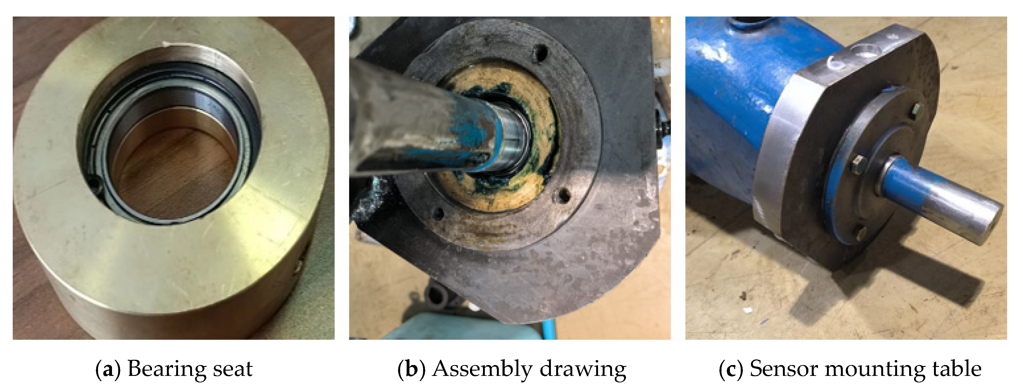
4.1.1. Experimental Platform

The centrifugal pump used in this experiment is the IS 100-80-160, which features a mature hydraulic design and is widely used in various applications. Being a medium-to-low specific speed centrifugal pump, it was chosen as the focus of this study due to its versatility. Figure 2 and Figure 3 depict the structural diagrams of the bearing experiment bench and sensor installation bench of the centrifugal pump.

A defective bearing was created during the experiment by using a laser to produce a specific defect at a designated location. The defect’s width and depth were denoted as B and H, respectively. Ultimately, two bearings with defective inner rings and one bearing with a defective outer ring were obtained. Figure 4 illustrates the defect location and the reassembled bearing.

4.1.2. Experimental Data Analysis

(1)

Time-domain feature analysis

The time-domain feature is the most direct, simplest, and most commonly used feature index. The specific information about the time-domain index selected in this paper is shown in

Table 1. Specific information on time-domain characteristic indicators.

Serial Number	Feature
T1	average
T2	standard deviation
T3	square root amplitude
T4	RMS (root mean square)
T5	peak-to-peak
T6	Skewness
T7	Kurtosis
T8	crest factor
T9	margin factor
T10	form factor
T11	pulse index

.

Figure 5 reveals that the amplitudes of the 11 time-domain characteristics differ. However, the time-domain characteristic amplitudes of the 11 normal bearing signals exhibit a trend of 1.0Q₀ < 0.8Q₀ < 1.4Q₀ < 0.4Q₀ under different operating conditions. The normal bearing signal‘s time-domain characteristic amplitude is the smallest, and it increases as the unit deviates further from the rated working condition until it reaches a maximum under the 0.4Q₀ working condition. This is due to the centrifugal pump impeller’s stable internal flow state and minimal disturbance under the rated working conditions, enabling the unit to operate smoothly. As the unit’s vibration increases, the amplitude also increases. When comparing the normal bearing signal’s time-domain characteristic amplitudes with those of the faulty time-domain characteristics, it is evident that the fault time-domain characteristic amplitudes are larger than the normal time-domain characteristic amplitudes under all four working conditions. The difference is most prominent at the rated operating point and gradually reduces with increasing levels of deviation. This may be due to the bearing failure weakening the shaft’s supporting effect and the fluid’s load on the impeller increasing during the deviation, resulting in increased vibration and masking fault signatures.

Overall, there is a significant difference between the normal characteristic and fault characteristic amplitudes of the time-domain signal; the performance of the time-domain signal under different working conditions is also inconsistent. Alternative features in the remaining life prediction schemes are needed.

(2)

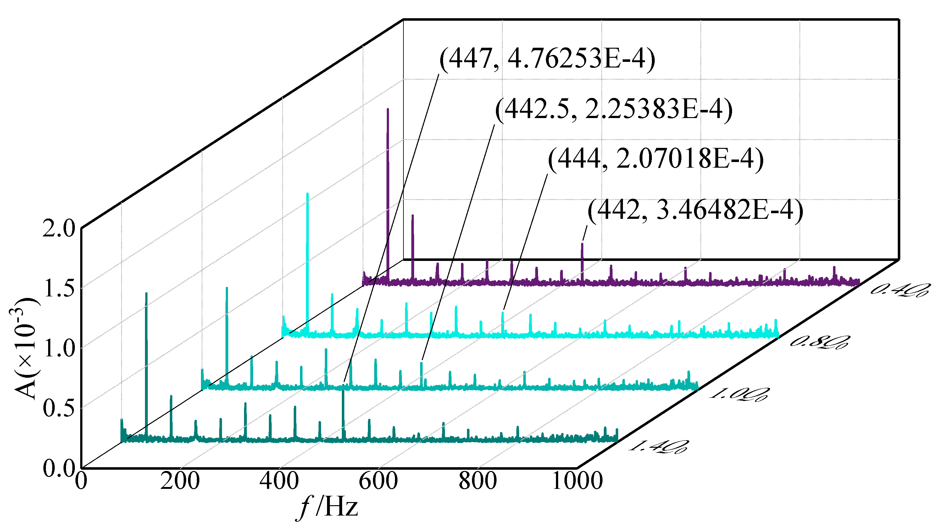
Frequency-domain feature analysis

Frequency-domain waterfall diagrams were produced for both normal and faulty bearings of centrifugal pumps operating under four different conditions, as depicted in Figure 6 and Figure 7.

The frequency spectrum of normal bearings operating under the four different conditions is primarily dominated by the rotation frequency, with a small peak at double the frequency of the rotation frequency. The peak pattern observed in the frequency domain analysis is consistent with that of the time domain analysis, with the fundamental frequency amplitude being most prominent during off-duty conditions. On the other hand, the faulty bearing’s frequency is not only prominent at the one-fold frequency position but also accompanied by frequencies that are two, three, and four times higher. This indicates that centrifugal pump failure leads to a significant increase in frequency multipliers. To determine the location of the faulty bearing’s damage, it is necessary to calculate its fault characteristic frequency. The calculated fault characteristic frequency for the bearing’s outer ring is 445.61 Hz. Comparing this with Figure 7, it is evident that the amplitude of the 0.4Q₀ working condition is most prominent at 442 Hz, the 0.8Q₀ working condition’s amplitude is most prominent at 444 Hz, the 1.0Q₀ working condition’s amplitude is most prominent at 442.5 Hz, and the 1.4Q₀ working condition’s amplitude is most prominent at 447 Hz. These results suggest that all four working conditions are near the fault frequency value of the bearing’s outer ring, indicating that the outer ring is faulty. Comparing the frequency-domain graph under normal and faulty conditions, it is evident that the frequency amplitude generally increases during the faulty condition and is accompanied by a prominent double frequency, with significant differences observed in the frequency domain. Therefore, frequency-domain analysis can effectively detect centrifugal pump bearing damage; its characteristics can be used as input for network models to predict the remaining life of the bearing.

(3)

Characteristic Analysis of Wavelet Packet Decomposition

The normal bearing operating under the 1.0Q₀ working condition was subjected to wavelet packet decomposition, and the resulting time-domain diagram of the eight frequency bands is presented in Figure 8. The X (3, 1) frequency band exhibited a higher and denser amplitude compared to other frequency bands, indicating that the energy density of normal bearings is higher in the low-frequency band.

When a bearing is damaged, its energy will suddenly change in some frequency bands. By comparing the energy characteristics of the frequency bands, the bearing’s fault type and degree of damage can be determined [12]. Since the energy feature is the sum of the information from each frequency band, the energy features of the eight sub-bands were selected as candidate features for predicting the remaining life of the centrifugal pump bearing.

(4)

CEEMDAN characteristic analysis

Figure 9 displays the results of the CEEMDAN decomposition performed on data collected under the normal bearing working condition (1.0Q₀). CEEMDAN was able to divide non-stationary and nonlinear data into multiple intrinsic mode functions (IMFs) with a single feature. A total of 11 IMF components and 1 residual item (RES) were decomposed, with each IMF component exhibiting relatively independent characteristics and no modal stacking phenomenon, resulting in good recognition performance. IMF1 and IMF2 contained more data points and larger amplitudes, while the trends of IMF8, IMF9, and IMF10 were similar, with amplitudes gradually decreasing until the trend of IMF11 showed a monotonous trend, indicating the end of decomposition.

To further analyze the difference between normal and faulty bearing signals of centrifugal pumps operating under different conditions in the CEEMDAN decomposition, the energy characteristics of the IMF components of each layer were extracted for comparative analysis. This was performed on both normal and faulty bearings under different working conditions. The results are presented in Figure 10.

Figure 10 shows that the amplitudes of the IMF1 and IMF5 components are relatively high under each working condition, indicating that the vibration signal of the centrifugal pump bearing is more sensitive to these components. Comparing the energy characteristics of IMF1 and IMF5 in the fault state and the normal state, it is evident that the amplitude of the IMF component in the fault state is significantly higher, particularly under the conditions of 0.8Q₀ and 1.0Q₀. Observing the IMF11 component, it is apparent that this component is only prominent at 0.8Q₀ and 1.0Q₀, with its amplitude being close to 0 at 0.4Q₀ and 1.4Q₀, indicating that the IMF11 component is more sensitive to changes in working conditions. The overall analysis suggests that some energy features decomposed by CEEMDAN are sensitive to faults and working conditions and can be used as candidate features in the remaining life prediction scheme of centrifugal pump bearings.

4.2. Verification of the Bearing Remaining Life Prediction Model

4.2.1. Experiment Platform

Since the research objects are all rolling bearings and only the influence of radial force is considered, the XJTU-SY open source data set is cited, and the test uses a bearing accelerated life test rig. In the test, the full life test of rolling bearings was carried out under three types of working conditions with different speeds and radial forces, and the vibration acceleration data of the bearings from the beginning of operation to damage were collected. Among them, 5 tests were done for each type of working conditions, and the establishment of Five sets of full-cycle life damage data sets were obtained. Since the characteristic trends of the three types of working conditions of the XJTU-SY data are basically the same, the data of working condition 1 are used for analysis. The specific information is shown in

Table 2. XJTU-SY bearing data set information.

Condition	Bearing Number	Total Number of Samples	Actual Life	Failure Location
Speed: 2100 (r/min) Radial force: 12 kN	A1	123	2 h 3 min	Outer ring
	A2	161	2 h 41 min	Outer ring
	A3	158	2 h 32 min	Outer ring
	A4	122	2 h 2 min	Cage
	A5	52	52 min	inner ring, outer ring

, and the experimental setup is shown in Figure 11 [2].

Figure 10 illustrates that the amplitudes of the IMF1 and IMF5 components are significantly higher under each working condition, indicating that these components are more sensitive to the vibration signal of the centrifugal pump bearing. When comparing the energy characteristics of IMF1 and IMF5 in the fault and normal states, it becomes evident that the IMF component’s amplitude is notably higher in the fault state, particularly under the 0.8Q₀ and 1.0Q₀ conditions. The IMF11 component is only prominent at 0.8Q₀ and 1.0Q₀, with its amplitude approaching 0 at 0.4Q₀ and 1.4Q₀, suggesting that this component is more sensitive to changes in working conditions. Overall, the analysis suggests that some energy features derived from CEEMDAN are sensitive to faults and working conditions and can be considered candidate features in the remaining life prediction scheme for centrifugal pump bearings.

4.2.2. Experimental Data Analysis

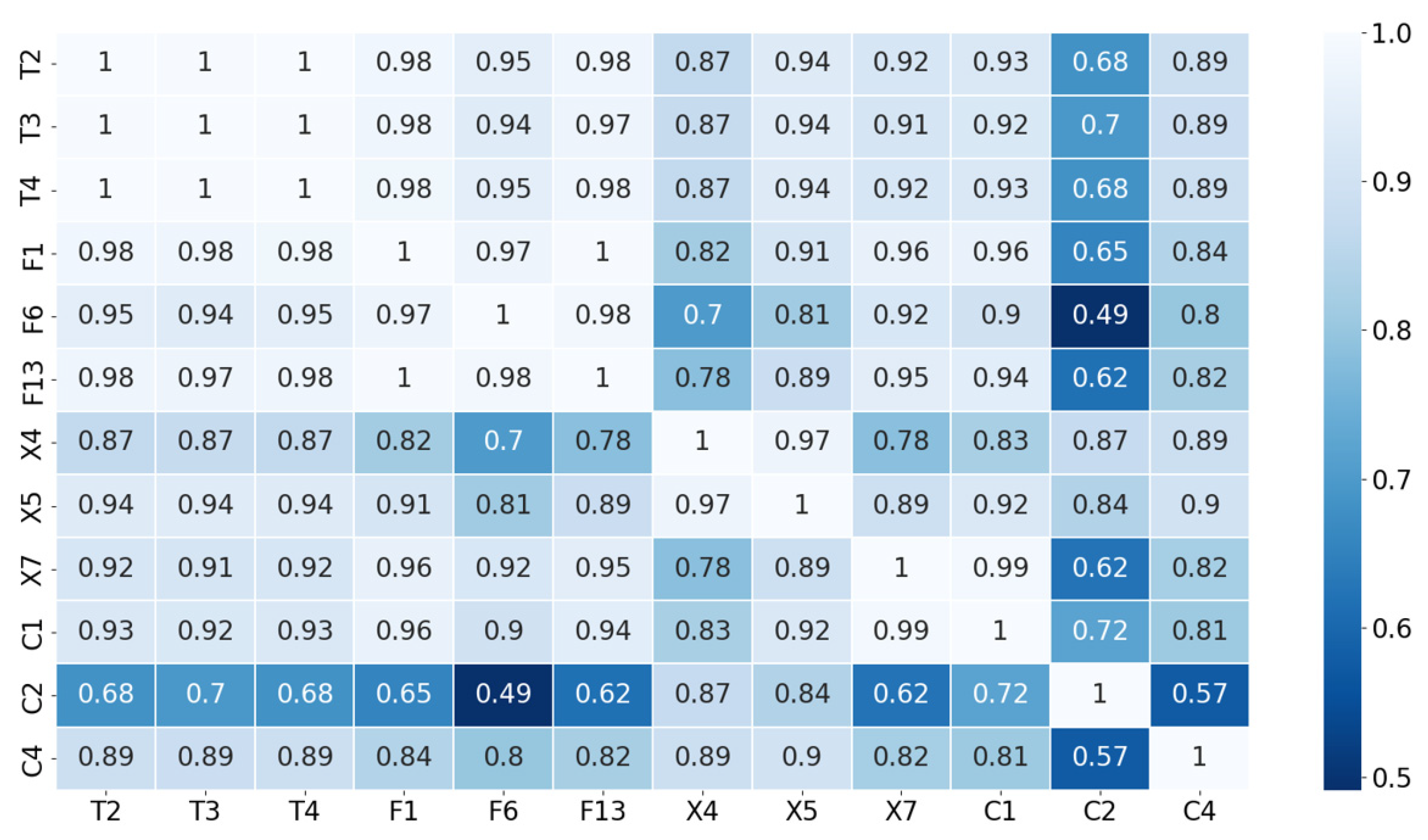
Based on the aforementioned analysis, time-domain features, frequency-domain features, energy features derived from wavelet packet decomposition, and energy features derived from the CEEMDAN decomposition can serve as indicators of the life degradation of bearings. Therefore, in this study, datasets A1, A2, A3, A4, and A5 were extracted, consisting of time-domain features, frequency-domain features, energy features derived from wavelet packet decomposition, and energy features derived from the CEEMDAN decomposition, for subsequent analysis. To better distinguish sensitive features in the rolling-bearing degradation process, three evaluation indices, namely monotonicity, trend, and robustness, were established for feature screening.

(1)

Monotonicity

The bearing degradation process can be described as a monotonically decreasing function, so it is necessary to use the monotonicity index to measure the quality of the feature. The calculation formula for the monotonicity index is as follows:

$$\begin{array}{c}Mon\left(F\right)=\left|\frac{C(\frac{d}{d{f}_i}>0)}{N-1}-\frac{C(\frac{d}{d{f}_i}<0)}{N-1}\right|\end{array}$$

(13)

In the formula, C stands for count, and N is the number of samples.

(2)

Trend

The bearing degradation process is strongly related to time, so the trend index is used to measure the correlation between characteristics and time, and its calculation formula is as follows:

$$\begin{array}{c}Tre\left(F,T\right)=\frac{\left|N{{\displaystyle \sum }}_i{f}_i{t}_i-{{\displaystyle \sum }}_i{f}_i{{\displaystyle \sum }}_i{t}_i\right|}{\sqrt{\left[N{{\displaystyle \sum }}_i{f}_i^2-{\left({{\displaystyle \sum }}_i{f}_i\right)}^2\right]\left[N{{\displaystyle \sum }}_i{t}_i^2-{\left({{\displaystyle \sum }}_i{t}_i\right)}^2\right]}}\end{array}$$

(14)

In the formula, f_i represents the feature sequence and t_i represents the time series, and the two correspond to each other.

(3)

Robustness

The bearing degradation process also needs to have good independence, so the robustness index is used to measure the anti-interference ability of the feature, and its calculation formula is:

$$\begin{array}{c}Rob=\frac{1}{N}{\displaystyle {\displaystyle \sum }_i}exp\left(\frac{f_i-\widetilde{f_i}}{f_i}\right)\end{array}$$

(15)

In the formula, ${\tilde{f}}_i$ is $f_i$ the smoothed trend item.

Based on the above analysis, we extracted a total of forty-three features, including eleven time-domain features, thirteen frequency-domain features, eight energy features derived from wavelet packet decomposition, and eleven energy features derived from the CEEMDAN decomposition. For each feature, its trend and robustness were calculated, and a monotonicity score was assigned. We then computed the comprehensive index score by adding the weighted scores of each feature. Finally, we plotted line charts for the trend score (Tre), robustness score (Rob), monotonicity score (Mon), and comprehensive index score (Com) of the 43 features, as shown in Figure 12.

Figure 12 indicates that the overall robustness score is relatively high, which can be attributed to the minimal interference of the experimental environment in the XJTU-SY dataset, leading to the data’s inherent robustness. Moreover, the monotonicity score of the bearing features is notably lower than the trend and robustness indices, mainly owing to the complex and prolonged degradation of the bearings that cannot be accurately measured by a single factor. Therefore, it is necessary to further process the features. To integrate the time-domain, frequency-domain, wavelet packet decomposition, and CEEMDAN decomposition features, we selected 12 features based on their comprehensive indicators, including three time-domain features, frequency-domain features, wavelet packet decomposition features, and CEEMDAN decomposition features. Since the comprehensive index scores of the fourth and fifth components decomposed by the CEEMDAN method are similar, we opted for the energy characteristics of the fifth component based on the aforementioned feature analysis results. The specific information regarding the preferred features is presented in

Table 3. Preferred Feature Specific Information.

Serial Number	Trend Score	Robustness Score	Monotonicity Score	Comprehensive Index Score
T2	0.863	0.898	0.302	0.533
T3	0.856	0.907	0.273	0.516
T4	0.863	0.898	0.302	0.533
F1	0.893	0.905	0.325	0.554
F6	0.904	0.939	0.299	0.548
F13	0.902	0.923	0.312	0.552
X4	0.772	0.853	0.266	0.485
X5	0.886	0.856	0.231	0.487
X7	0.881	0.827	0.263	0.499
C1	0.890	0.837	0.269	0.507
C2	0.830	0.858	0.201	0.458
C5	0.683	0.856	0.133	0.388

, where Xi and Ci indicate the i-th layer energy features after the wavelet packet decomposition and the CEEMDAN decomposition, respectively.

From the table, we can see the trend, robustness, and monotonic scores of the preferred features, but they cannot reflect the correlation between features. To do this, the correlation coefficient between the features is calculated, and the expression is as follows:

$$\begin{array}{c}{\rho }_{xy}=\frac{Cov\left(x,y\right)}{\sqrt{Dx,Dy}}\end{array}$$

(16)

In the formula, $\rho$ is the correlation coefficient, and Cov is the covariance.

By applying the formula, we can calculate the correlation coefficient between the features and plot a heat map, as shown in Figure 13. The figure reveals that the time-domain features exhibit strong correlation characteristics, primarily due to their predominantly linear functional relationship. In general, the correlation coefficients between each feature and the time-domain feature are above 0.6, indicating a strong correlation between the optimal feature and time, which can be utilized to reflect the relationship between life degradation and time of bearings. In contrast, the correlation between each feature and the energy features obtained through the CEEMDAN decomposition is weak, implying that the features derived from the CEEMDAN decomposition are more independent.

Based on the aforementioned analysis, it is evident that the preferred features possess certain advantages in terms of trend, robustness, and monotonicity. Furthermore, each feature maintains a certain degree of independence while exhibiting a strong correlation with time, thereby satisfying the criteria for feature screening and facilitating subsequent feature fusion. To reduce the dimensionality of the selected 12 features, we performed KPCA based on the aforementioned steps and obtained single-dimensional data. To enhance the prediction accuracy and standardize the data, we normalized the data. The resulting XJTU-SY dataset obtained under unified working conditions for the five rolling degradation samples of the bearings is illustrated in Figure 14.

Figure 14 shows that the trend index generated through feature fusion exhibits a different service life when damaged and typically displays a monotonically increasing trend. This finding aligns with the discrete nature of rolling-bearing life and the characteristics of the degradation process. Thus, the constructed bearing life-degradation trend index retains the information of the original signal and conforms to the law of bearing life-degradation. It can serve as an input for predicting the remaining life of centrifugal pump bearings.

4.3. Centrifugal Pump Rolling-Bearing Life Prediction

In order to better compare the prediction results, the root mean square error (RMSE) and the mean absolute percentage error (MAPE) are used to measure the prediction accuracy, and the expressions are as follows [14]:

$$\begin{array}{c}\mathrm{RMSE}=\sqrt{\frac{1}{n}\times {\displaystyle {\displaystyle \sum }_{i=1}^n}{\left(X_i-P_i\right)}^2}\end{array}$$

(17)

$$\begin{array}{c}\mathrm{MAPE}={\displaystyle {\displaystyle \sum }_{i=1}^n}\left|\frac{X_i-P_i}{P_i}\right|\times \frac{1}{n}\end{array}$$

(18)

In the formula, n is the number of experiment samples, and X_i and P_i are the true and predicted values of all experiment samples, respectively.

The model’s prediction performance is evaluated based on the RMSE and MAPE values, where lower values indicate a better prediction effect. To comprehensively evaluate the bearing remaining life prediction scheme, a full life cycle verification analysis is conducted using degradation data collected from the beginning of the operation to the point of damage to the rolling bearing. By employing the full life cycle data, we can capture all the information regarding bearing degradation, which is beneficial for accurately predicting the remaining life of centrifugal pump bearings.

Table 4. Full life cycle data training and prediction-specific information.

Sample	RMSE	MAPE	T (s)
A3	0.155	0.386	28.8
A4	0.072	0.272	28.8
A5	0.112	0.233	28.8

presents the RMSE, MAPE, and model training time (T) of samples A3, A4, and A5 predicted using the full life data of samples A1 and A2 under working conditions. The results indicate that, compared with single-sample prediction, the LSTM network significantly improves the prediction accuracy of each sample, even though it does not have access to A3, A4, and A5 sample data. This finding demonstrates that the constructed centrifugal pump bearing degradation trend can reflect the common characteristics of bearings with different fault locations and damage times. Overall, the LSTM model performs better in predicting the entire cycle when supported by the degradation data of the bearing’s entire life.

Figure 15 is the effect diagram of training and prediction, in which Train reflects the training situation of the LSTM network for A1 and A2 working condition data. Predicted A3, A4, and A5 reflect the prediction of the sample.

Figure 15 depicts the prediction results of the LSTM network model. The model exhibits good prediction performance when the bearing fails early; however, when the bearing fails severely, its degradation process undergoes a sudden change, and the trend abruptly shifts at a certain moment. Upon comparing several prediction samples, we observed that the uncertainty associated with this sudden change is most pronounced when predicting sample A4, which directly contributes to the reduction of the LSTM model‘s prediction accuracy at that point. Nevertheless, compared with single-sample prediction, the LSTM model’s accuracy has been significantly improved. Furthermore, the model’s prediction accuracy increases with the amount of training data, allowing it to better predict the remaining life of the bearing.

5. Conclusions

This paper proposes a KPCA–LSTM prediction scheme for predicting the remaining life of centrifugal pump bearings using a data-driven approach. Our research demonstrates that time-domain features, frequency-domain features, wavelet packet decomposition energy features, and CEEMDAN energy features can capture fault information under different working conditions, but only a few features remain sensitive during the life cycle of centrifugal pump bearings. Therefore, we selected 12 outstanding features and used the KPCA algorithm to construct a one-dimensional feature quantity that characterizes the degradation process of the centrifugal pump bearing. This feature quantity was then input into the LSTM network for prediction and analysis. The results indicate that the LSTM network outperforms other models in terms of prediction accuracy and model training time, and its accuracy continues to improve with increasing amounts of training data.

References

1. Mand Hare, A.; Karunamurthy, K.; Ismail, S. Compendious review on “Internal Flow Physics and Minimization of Flow Instabilities Through Design Modifications in a Centrifugal Pump”. J. Press. Vessel. Technol. 2019, 141, 5–16. [Google Scholar]
2. Lei, Y.G.; Han, T.Y.; Wang, B.; Li, N.; Yan, T.; Yang, J. Interpretation of XJTU-SY Rolling Bearing Accelerated Life Test Dataset. Chin. J. Mech. Eng. 2019, 55, 1–6. [Google Scholar]
3. Guo, Z.; Li, Y.; Li, G. Research progress on equipment system remaining service life prediction technology. J. Nanjing Univ. Aeronaut. Astronaut. 2022, 54, 341–364. [Google Scholar]
4. Khalid, S.; Khalil, T.; Nasreen, S. A survey of feature selection and feature extraction techniques in machine learning. In Proceedings of the 2014 Science and Information Conference, London, UK, 27–29 August 2014; pp. 372–378. [Google Scholar]
5. Pei, H.; Hu, C.; Si, X. Review of machine learning-based equipment remaining life prediction methods. Chin. J. Mech. Eng. 2019, 55, 1–13. [Google Scholar] [CrossRef]
6. Lu, N.; Li, T.; Ren, X.; Miao, H. A deep learning scheme for motor imagery classification based on restricted Boltzmann machines. IEEE Trans. Neural Syst. Rehabil. Eng. 2016, 25, 566–576. [Google Scholar] [CrossRef] [PubMed]
7. Khan, A.; Sohail, A.; Zahoora, U.; Qureshi, A.S. A survey of the recent architectures of deep convolutional neural networks. Artif. Intell. Rev. 2020, 53, 5455–5516. [Google Scholar] [CrossRef]
8. Weerakody, P.B.; Wong, K.W.; Wang, G.; Ela, W. A review of irregular time series data handling with gated recurrent neural networks. Neurocomputing 2021, 441, 161–178. [Google Scholar] [CrossRef]
9. Lu, W.; Duan, J.; Wang, P.; Ma, W.; Fang, S. Short-term wind power forecasting using the hybrid model of improved variational mode decomposition and Correntropy Long Short-term memory neural network. Energy 2021, 214, 118980. [Google Scholar] [CrossRef]
10. Schölkopf, B.; Smola, A.; Müller, K.R. Nonlinear component analysis as a kernel eigenvalue problem. Neural Comput. 1998, 10, 1299–1319. [Google Scholar] [CrossRef]
11. Zhang, Y.; Zheng, J.; Jiang, Y.; Huang, G.; Chen, R. A text sentiment classification modeling method based on coordinated CNN-LSTM-Attention model. Chin. J. Electron. 2019, 28, 120–126. [Google Scholar] [CrossRef]
12. Li, S.; Li, Z.; Li, H. Rolling bearing fault monitoring method based on wavelet packet energy characteristics. J. Syst. Simul. 2003, 15, 6. [Google Scholar] [CrossRef]
13. Wang, B.; Lei, Y.; Li, N.; Li, N. A Hybrid Prognostics Approach for Estimating Remaining Useful Life of Rolling Element Bearings. IEEE Trans. Reliab. 2020, 69, 401–412. [Google Scholar] [CrossRef]
14. Luo, X. Forecasting Foreign Exchange Rate Based on Convolutional Neural Network; Guizhou University: Guiyang, China, 2020. [Google Scholar]
Figure 1. STM structure diagram.
Energies 17 04167 g001
Figure 2. IS 100-80-160 centrifugal pump bearing experiment bench.
Energies 17 04167 g002
Figure 3. Structural diagram of the bearing seat and sensor mounting table.
Energies 17 04167 g003
Figure 4. Faulty bearing.
Energies 17 04167 g004
Figure 5. Comparison of time-domain characteristics of centrifugal pumps under different working conditions.
Energies 17 04167 g005
Figure 6. Frequency-domain waterfall diagram of normal bearing under different working conditions.
Energies 17 04167 g006
Figure 7. Waterfall diagram of fault bearing in the frequency domain under different working conditions.
Energies 17 04167 g007
Figure 8. Decomposition of a wavelet packet in the 1.0Q0 working condition of a normal bearing.
Energies 17 04167 g008
Figure 9. CEEMDAN decomposition results of a normal bearing or 1.0Q0 working condition.
Energies 17 04167 g009
Figure 10. Comparison of energy characteristics of CEEMDAN in normal and fault states under different working conditions.
Energies 17 04167 g010
Figure 11. XJTU-SY bearing accelerated-life experiment bench [3,13].
Energies 17 04167 g011
Figure 12. Score map of the bearing characteristic index.
Energies 17 04167 g012
Figure 13. Heat map between preferred features.
Energies 17 04167 g013
Figure 14. XJTU-SY data set operating condition-trend index.
Energies 17 04167 g014
Figure 15. Full life cycle data training and prediction effect.
Energies 17 04167 g015