Slow-Scale Bifurcation Analysis of a Single-Phase Voltage Source Full-Bridge Inverter with an LCL Filter

Abstract

In high-power photovoltaic systems, the inverter with an LCL filter is widely used to reduce the value of output inductance at which a lower switching frequency is required. However, the effect on the stability of the system caused by an LCL filter due to its resonance characteristic cannot be ignored. This paper studies the stability of a single-phase voltage source full-bridge inverter with an LCL filter through the bifurcation theory as it is a nonlinear system. The simulation results show that low-frequency oscillation appears when the proportional coefficient of the system controller increases or the damping resistance decreases to a certain extent. The average model is derived to analyze the low-frequency oscillation; the theoretical analysis demonstrates that low-frequency oscillation is essentially a period in which doubling bifurcation occurs, which indicates the intrinsic mechanism of the instability of the full-bridge inverter with an LCL filter. Additionally, the limitation of the existing damping resistor design standards, which only considers the main circuit parameters but ignores the influence of the controller on system stability, is identified. To solve this problem, the analytical expression of the system stability boundary is provided, which can not only provide convenience for engineering design to protect the system from low-frequency oscillation but also expand the selection range of damping resistance in practice. The experiments are performed to verify the results of the simulation and theoretical analysis, demonstrating that the analysis method can facilitate the design of the inverter with an LCL filter.

1. Introduction

With the development of photovoltaic (PV) power generation technology, the high-power photovoltaic power system in which a lower switching frequency is employed by the inverter to reduce the switching loss and electromagnetic interference is becoming increasingly prevalent [1,2]. In order to meet the harmonics requirements, a high output inductance should be used, which will not only increase the filter volume but also weaken the system’s dynamic response. An attractive solution for this problem is to use an LCL filter [3,4,5].

However, the resonance characteristic of the LCL filter directly affects the stability of the inverter, consequently affecting the stable operation of the entire system [6,7,8]. The most effective method to suppress the resonance characteristics is to increase the damping resistance. Considering the influence of the filter inductance values, the filter capacitance, and the inverter switching frequency, six typical passive damping methods have been studied by adding series or paralleled resistors to the LCL filter branches in [9]. Compared with other typical passive damping methods, the damping resistors in series with the capacitor C are the most appropriate from the perspective of power losses. In ref. [10], to ensure the sufficient stability margin of the system, the minimum value of the damping resistor in series with the capacitor is adopted as 20% of the capacitor impedance at the resonance frequency. In grid inverters with LCL filters, the wide range variation of grid impedance may bring a wide range of variation in the resonance frequency, which will result in instability in the system [11].

In addition, a lot of research on the stability of inverters with LCL filters has been carried out [12,13,14,15]. In ref. [12], a deep reinforcement learning-based proportional-resonant controller is proposed to improve the stability of the system under different operating conditions, and the efficacy of the proposed method is verified by the experimental results; in ref. [13], an impedance–resonance analysis method is proposed to observe the reason for the resonances; in ref. [14], the influence of the LCL parameters on the stability of the inverter is studied, and the results show that the system stability is related to the d-d channel output admittance of the inverter and the inductive component of the grid impedance; and in ref. [15], the mechanism of high-frequency resonance in a three-phase LCL photovoltaic grid-connected inverter system is revealed, and an active damping design method was also proposed to suppress harmonic resonance.

These studies on the stability of the system are always based on the linear theory, while the inverter is a type of strongly nonlinear system, so the complex nonlinear phenomena that affect the performance of the inverter should not be neglected [16,17,18,19]. Recently, studies on the nonlinear dynamics of power electronic circuits have indicated that bifurcation behavior in power electronic circuits can lead to significant noise and unstable behavior, which is very harmful in practical applications. Therefore, bifurcation behavior should be avoided as much as possible. However, if the parameters of the system design are too far from the bifurcation boundary, it will also reduce performance indicators, such as the transient response speed of the system. By analyzing this complex nonlinear phenomenon, more effective control strategies can be developed to reduce low-frequency oscillations and other unstable phenomena, thereby improving the dynamic response of the system [20,21]. On this basis, it is necessary to study the dynamic behaviors of the inverter with an LCL filter.

At present, several studies have been focused on the complex behaviors of inverters with L-type or LC-type filter circuits [22,23,24,25,26]. For instance, in refs. [22,23], the bifurcations of chaotic attractors in piecewise smooth maps with multiple switching manifolds were discussed. Taking inverters as the model, it is demonstrated that chaotic attractors within this model might contain regions with very low densities. In ref. [24], a slow-scale nonlinear control method of the H-bridge photovoltaic inverter was proposed to avoid slow-scale nonlinear behaviors. In ref. [25], the Hopf and saddle-node bifurcations were observed in the microgrid system, and the capability of the distributed secondary control in preventing the occurrence of bifurcation was verified by experiments. In ref. [26], the mechanism of the slow-scale and fast-scale behaviors of the single-phase H-bridge inverter were illustrated by the state space average model and the Filippov method, respectively.

However, few studies have been conducted on the bifurcation behaviors of the inverter with an LCL filter. The slow-scale bifurcation phenomenon of a digitally controlled inverter with an LCL filter under off-grid conditions was studied in ref. [27], considering the digital adoption delay, and it pointed out that the slow-scale instability of the system is actually Hopf bifurcation. This research adopted a discrete model to study the slow-scale behavior of the system, while not considering the influence of damping resistance on the stability of the system, which is directly affected by the damping resistance value.

This paper focuses on analyzing the slow-scale bifurcation phenomenon of a single-phase voltage source full-bridge inverter with an LCL filter. The simulations show that the slow-scale instability phenomenon occurs when improper parameters of the system are selected. Considering the nonlinear characteristics of inverters, a nonlinear analysis method is proposed to identify the mechanization of the slow-scale instability phenomenon. The theoretical analysis indicates that the slow-scale instability is essentially Hopf bifurcation occurs. In addition, it is pointed out that the existing traditional damping resistor design standard is insufficient for neglecting the influence of control parameters. Moreover, based on the established average model, the analytical stability boundary is derived, which will facilitate the selection of appropriate system parameters in engineering design to avoid the occurrence of slow-scale instabilities. Finally, the experiment results validate the correctness of the simulation results and theoretical analysis.

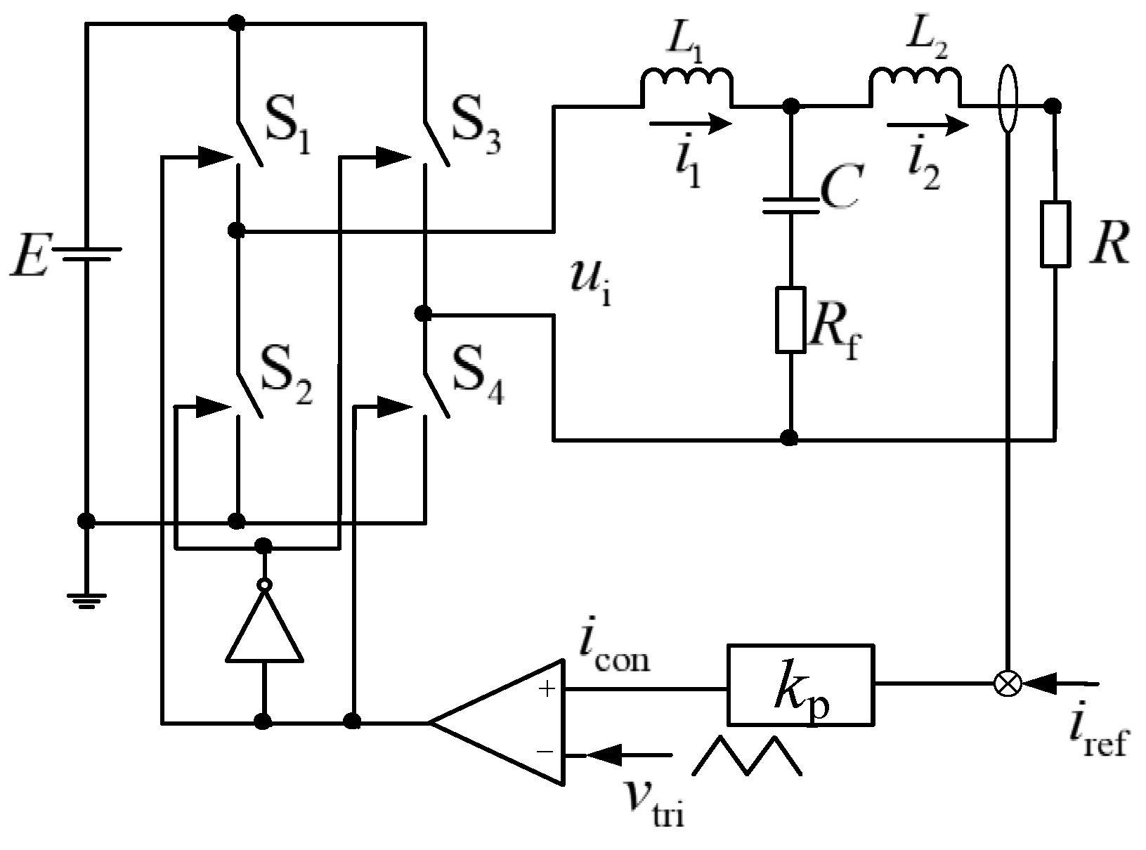
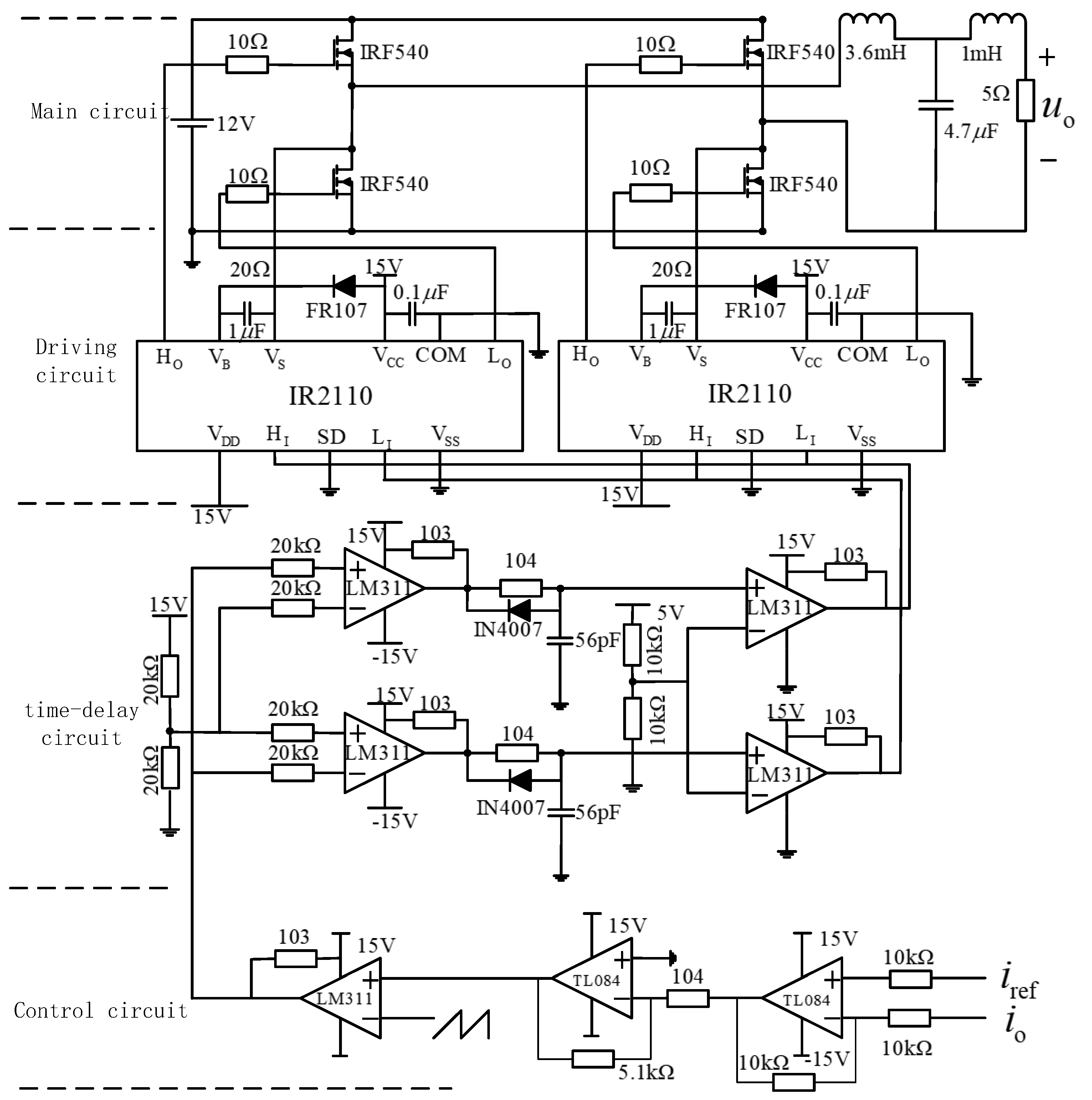
2. Circuit Description

2.1. Circuit Operation

The control signal i_con(t) is compared with the carrier signal v_tri(t) to generate a pulse signal for driving the switch S_j (j = 1, 2, 3, 4). The triangular wave carrier signal for each switching cycle is given as follows:

$$R_f\approx {\displaystyle \frac{1}{3w_{res}C}}$$

(1)

The control signal i_con(t) is compared with the carrier signal v_tri(t) to generate a pulse signal for driving the switch S_j (j = 1, 2, 3, 4). The carrier signal in each switching cycle is given as follows:

$$v_{\mathrm{tri} }(t)=\left\{\begin{array}{ll}-V_{\mathrm{tri} }+4V_{\mathrm{tri} }{\displaystyle \frac{t}{T_{\mathrm{s}}}},\hfill & 0<t\le {\displaystyle \frac{T_{\mathrm{s}}}{2}}\hfill \\ -V_{\mathrm{tri} }+4V_{\mathrm{tri} }{\displaystyle \frac{\left(T_{\mathrm{s}}-t\right)}{T_{\mathrm{s}}}},\hfill & {\displaystyle \frac{T_{\mathrm{s}}}{2}}<t\le T_{\mathrm{s}}\hfill \end{array}\right.$$

(2)

where −V_tri is the minimum value of the triangular wave, V_tri is the maximum value of the triangle wave, and T_s is the switching period.

2.2. State Equation

Referring to Figure 1, the circuit exhibits two switch states during a switching period.

State A: S₁ and S₄ are on, S₂ and S₃ are off.

State B: S₂ and S₃ are on, S₁ and S₄ are off.

According to the circuit topology in each state, the state equations of the inverter can be expressed as follows:

$$\left\{\begin{array}{l}{\displaystyle \frac{\mathrm{d}{u}_C}{ \mathrm{d}t}}={\displaystyle \frac{1}{C}}{i}_1-{\displaystyle \frac{1}{C}}{i}_2\hfill \\ {\displaystyle \frac{\mathrm{d}{i}_1}{ \mathrm{d}t}}=-{\displaystyle \frac{1}{L_1}}{u}_C-{\displaystyle \frac{R_{\mathrm{f}}}{L_1}}{i}_1+{\displaystyle \frac{R_{\mathrm{f}}}{L_1}}{i}_2+{\displaystyle \frac{(2S-1)E}{L_1}}\hfill \\ {\displaystyle \frac{\mathrm{d}{i}_2}{ \mathrm{d}t}}={\displaystyle \frac{1}{L_2}}{u}_C+{\displaystyle \frac{R_{\mathrm{f}}}{L_2}}{i}_1-{\displaystyle \frac{R_{\mathrm{f}}+R}{L_2}}{i}_2\hfill \end{array}\right.$$

(3)

where u_C is the capacitor voltage, i₁ is the inverter side inductive current, i₂ is the load side inductive current, R_f is the series resistance of the capacitor branch, S is the switching function (S = 1, circuit operating in state A; S = 0, the circuit works in state B), E is the DC-side voltage, and R is the load resistance.

The relationship between the control signal i_con and the load side inductor current i₂ is given as follows:

$$i_{\mathrm{con}}=k_{\mathrm{p}}\left(i_{\mathrm{ref}}-i_2\right)$$

(4)

where k_p is the proportional coefficient of the controller and i_ref is the reference value of the inverter load current.

2.3. Linearized Switching Model

According to the schematic diagram of the system shown in Figure 1, the linearized switching model of a single-phase voltage source full-bridge inverter with an LCL filter is as shown in Figure 2.

The transfer function relating the inductance current i₂ to the output voltage of the inverter u_i can be shown in Equation (5), as follows:

$$G_1(s)={\displaystyle \frac{i_2(s)}{u_i(s)}}={\displaystyle \frac{1}{L_1{L}_{2}Cs}}·{\displaystyle \frac{1+C{R}_{f}s}{s^2+w_{r\mathrm{es}}^2(1+C{R}_{f}s)}}$$

(5)

where $w_{r\mathrm{es}}=\sqrt{{\displaystyle \frac{L_1+L_2}{L_1{L}_{2}C}}}$.

The transfer function G_P (s) for the proportional controller is given as follows:

$$G_P(s)=k_p$$

(6)

The open-loop transfer function of the single-phase voltage source full-bridge inverter with an LCL filter can be expressed as follows:

$$G(s)={\displaystyle \frac{K_{PWM}{G}_P(s)(1+C{R}_{f}s)}{L_1{L}_{2}C{s}^3+(L_1+L_2)C{R}_f{s}^2+(L_1+L_2)s}}$$

(7)

3. Numerical Simulations

Based on the operating principle mentioned in Section 2, a series of simulations under different parameters are implemented using PSIM 9.1.4 to identify possible instabilities in a single-phase voltage source full-bridge inverter with an LCL filter. The specific parameters of the studied system are listed in

Table 1. Main simulation parameters.

Name	Simulation Parameter
DC-side voltage	E = 12 V
Load resistance	R = 5 Ω
Inverter LCL filter parameters	L1 = 3.6 mH, C = 4.7 μF, L2 = 1 mH
Carrier amplitude	Vtri = 1
Line frequency	f = 50 Hz
Invert switching frequency	fs = 10 kHz
Reference current amplitude	Iref = 1 A

. Actually, the stability of the system is always in regard to the control parameter k_p and the damping resistance R_f. Therefore, the dynamical behavior of the single-phase voltage source full-bridge inverter with an LCL filter is studied as k_p and R_f vary.

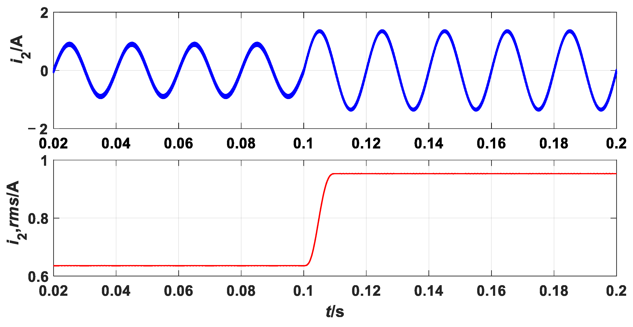
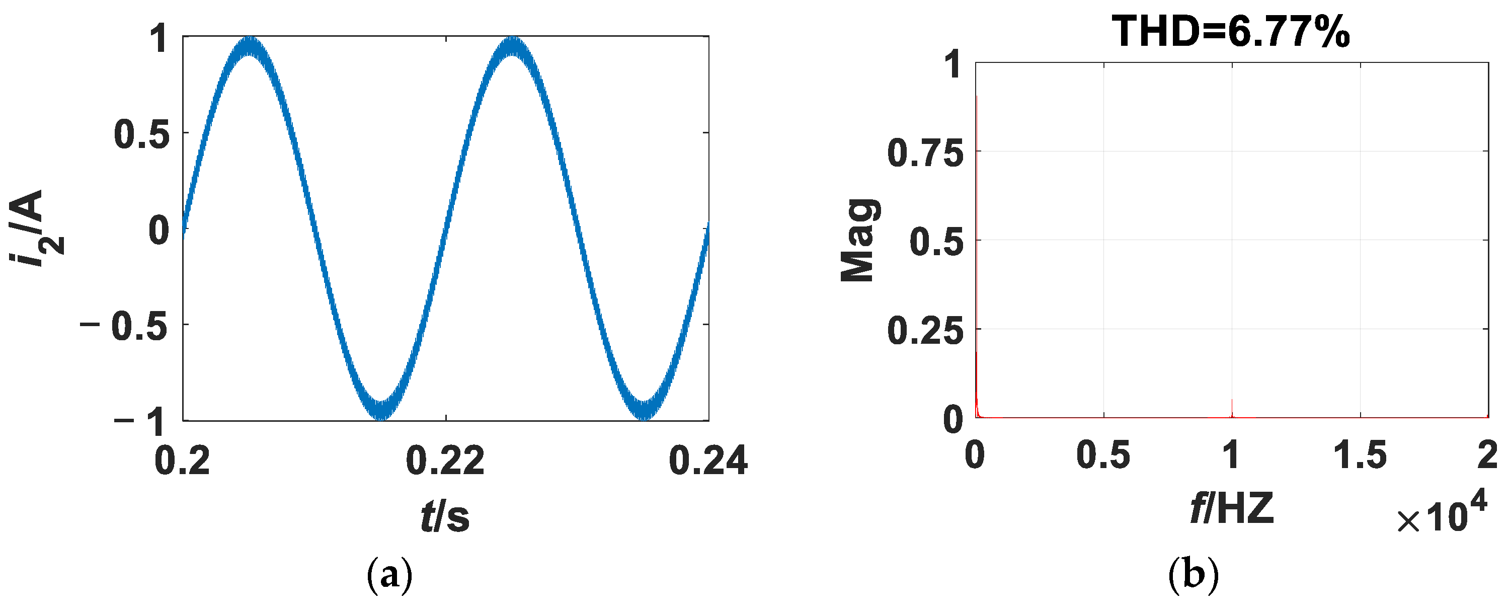
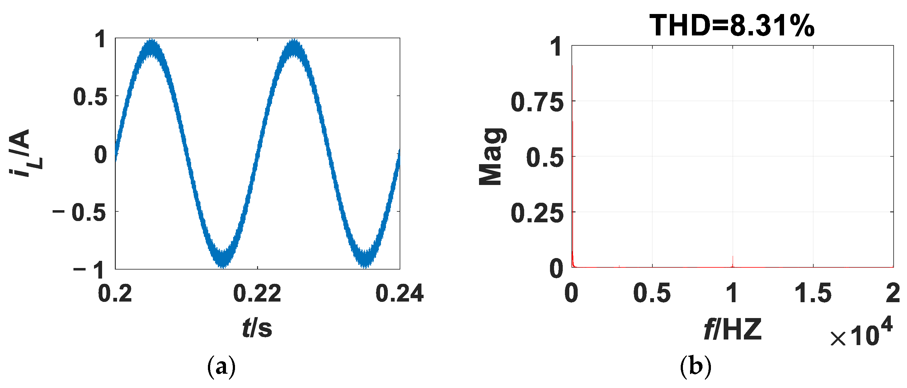
3.1. Transient-State Simulation

To identify the efficacy of the instantaneous response characteristic of the system, the simulation is carried out as the reference current increases by 50% at t = 0.1 s. The parameters used are as shown in Table 1, while k_p = 4.5. The inductor current and its root mean square are shown in Figure 3. It can be seen that the inductor current follows the increase in the reference current value smoothly without overshooting, and the duration of the transition process is less than 0.01 s, which reflects the fine transient characteristics of the system.

3.2. k_p as the Bifurcation Parameter

3.2.1. k_p as the Bifurcation Parameter

Based on the simulation parameters in Table 1, the value of the damping resistance R_f is set to 4.3 Ω according to Equation (4).

When k_p = 4.5, the operation state of the system is shown in Figure 4. In Figure 4a, it can be seen that the peak value of the inductor current i₂ is 1A and the line frequency is 50 Hz, which shows that the output current follows the reference current. In this situation, the time domain waveforms of the inductor current i₂ are smooth, which means that the system operates in a stable station. Figure 4b shows that the inverter only generates harmonics at 1 k Hz, which is just the switching frequency, and the total harmonic distortion (THD) is 6.77%, which is permitted with the resistance load.

As k_p increases to 4.72, the time domain wave of inductor current i₂ and its FFT are shown in Figure 5a and 5b, respectively. In Figure 5a, it can be seen that the inductor current i₂ oscillates slightly over the entire line cycle. Compared with Figure 4a, it can be seen that the circuit loses steady operation, which may bring harsh electromagnetic noise and oscillation of the system. Referring to the spectrum analysis, as shown in Figure 5b, it is seen that the oscillation frequency of the system is about 2.95 kHz, which is far less than the switching frequency, indicating that this oscillation is a low-frequency oscillation. Moreover, the THD value amounts to 8.31%, and the harmonic characteristics of the system are destroyed as the instability occurs.

With the increase in k_p, the low-frequency oscillation becomes more serious. As k_p continues to increase to 4.74, the time domain waveform of inductor current i₂ is shown in Figure 6a. It can be seen that the oscillation amplitude of the inductor current i₂ on the line cycle increases obviously, and the system works in an unstable state. Figure 6b is the frequency spectrum of inductor current i₂. Compared with Figure 5b, it can be found that the peak value of the low-frequency oscillation increases obviously, and the oscillation frequency is about 2.96 kHz. With the increasing oscillation, the THD value reaches 14.35%.

The simulation results above indicate that the voltage source full-bridge inverter with an LCL filter will lose its stable operation and transition into the low-frequency oscillation state as the control parameter k_p increases. Simultaneously, the THD value of the system rises obviously with the increasingly severe oscillation.

3.2.2. R_f as the Bifurcation Parameter

Keeping k_p = 4.5 constant and taking R_f as the bifurcation parameter, the influence of the damping resistance R_f on the system stability is analyzed. The simulation results for the case where R_f = 4.2 Ω are shown in Figure 5. Figure 7a,b show the time domain waveform of inductor current i_L and its FFT, respectively. It can be seen from Figure 7a that the inductor current i₂ does not oscillate and the waveform keeps consistent with the reference current so that the system operates in stable operation. As can be seen in Figure 7b, the system exhibits harmonics only at the switching frequency, which is similar to Figure 4b, also indicating a steady state operation; the THD value is 6.89% in this situation.

When R_f is reduced to 4.095 Ω, the inductor current i₂ loses its stability and oscillates slightly in the entire line cycle, as shown in Figure 8a, and the electromagnetic noise may arise here. Although the oscillation amplitude is relatively small, the THD value increases to 8.41%, as shown in Figure 8b. Furthermore, it can be seen in Figure 8b that the oscillation frequency is about 2.9 kHz, which is far from the switching frequency, indicating that the circuit enters into low-frequency oscillation from a stable state as the damping resistor R_f varies.

R_f continues to decrease when R_f = 4.06 Ω; the time domain waveform of the inductor current i₂ and its FFT are shown in Figure 9a and 9b, respectively. In Figure 9a, it can be seen that the oscillation amplitude of inductor current i₂ increases significantly compared with Figure 8a, and the electromagnetic noise can be more significant. Figure 9b shows that the system harmonics increase with the increasing oscillation intensity, and the oscillation frequency is 2.94 kHz.

It can be seen from the simulations above that the value of the damping resistance is extremely important in that it determines the resonance characteristics of the voltage source full-bridge inverter with an LCL filter. It is also obvious that the more severe the oscillation, the higher the THD value.

To compare the system status under different simulation parameters, a table based on the simulation results in Section 3.2 is listed as shown in

Table 2. System status under different simulation parameters.

kp	Rf	Simulation Results	System Status
4.5	4.3	not oscillate	stable
4.72		low-frequency oscillation	unstable
4.74		oscillation increases	unstable
4.5	4.2	not oscillate	stable
	4.095	low-frequency oscillation	unstable
	4.075	oscillation increases	unstable

. It is easy to see that the system will transition into unstable status when improper parameters are chosen, that is when k_p is too large or the R_f is too small.

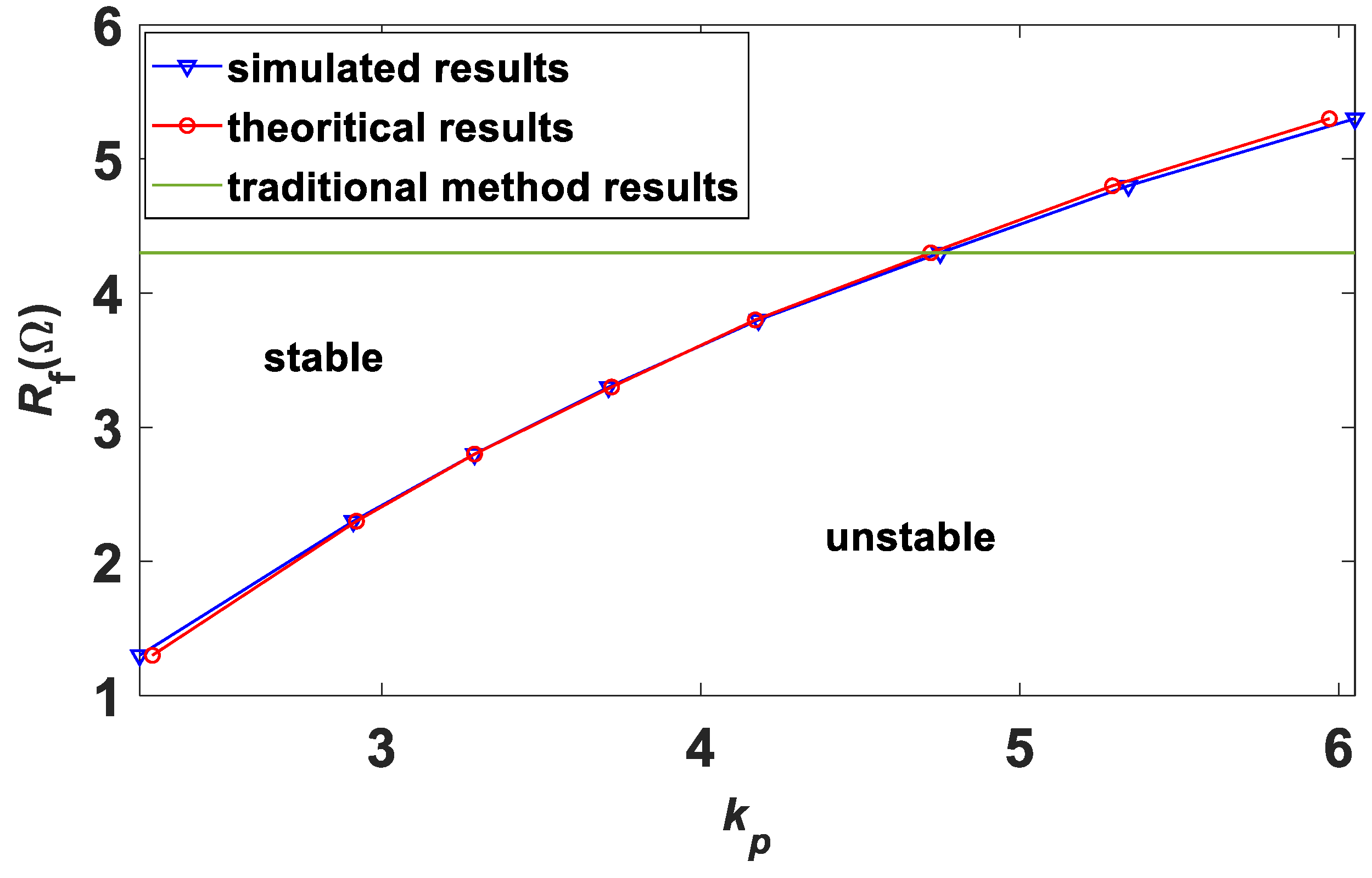
4. Theoretical Analysis

According to the abovementioned simulation results, the system loses its stability in the form of slow-scale oscillation under different parameters. Two methods of analysis will be adopted to obtain the mechanisms of the oscillation. Firstly, the stability is studied based on the linearized switching model using the frequency domine analysis method. Then, the averaged model is applied to analyze the low-scale instability.

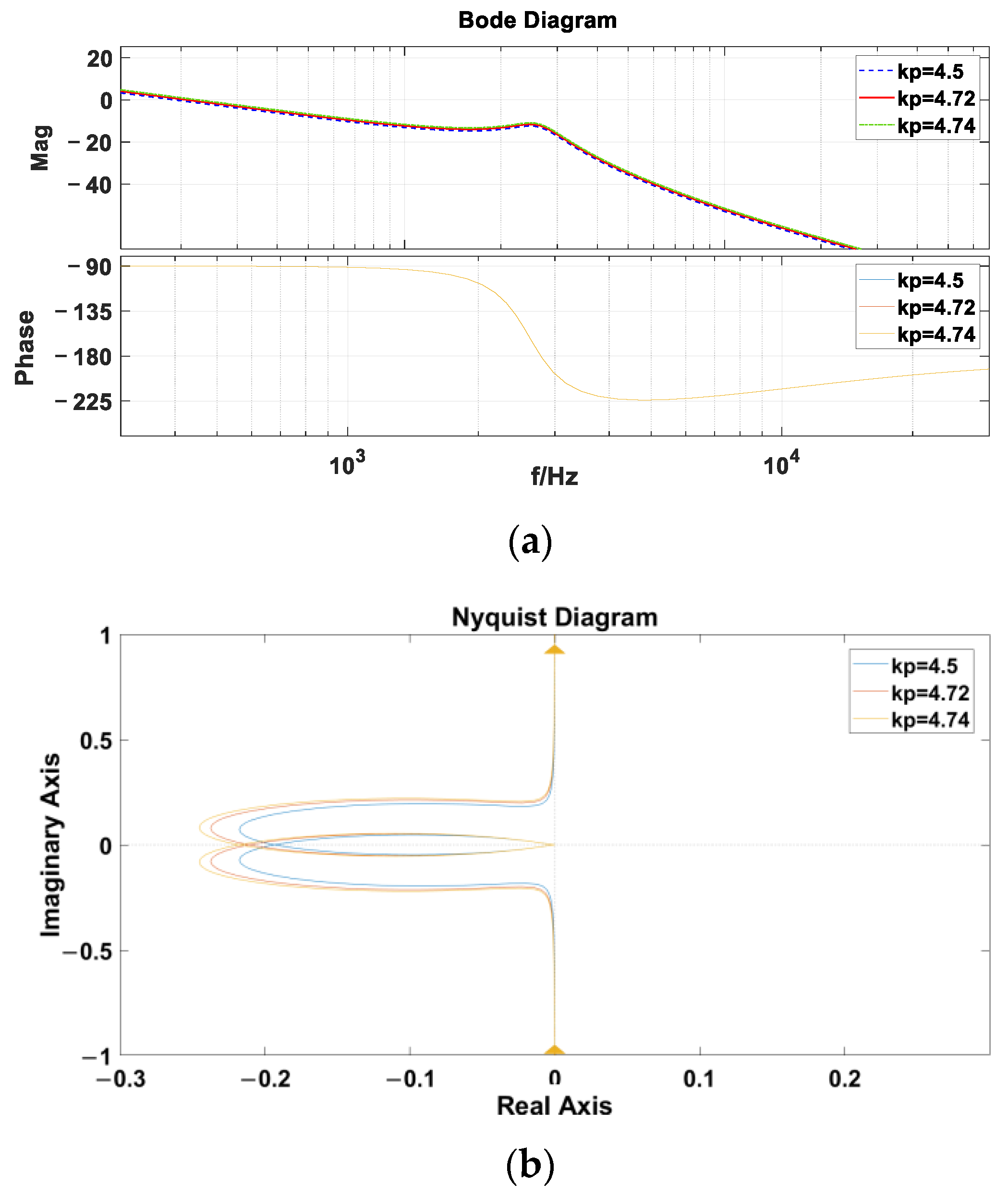
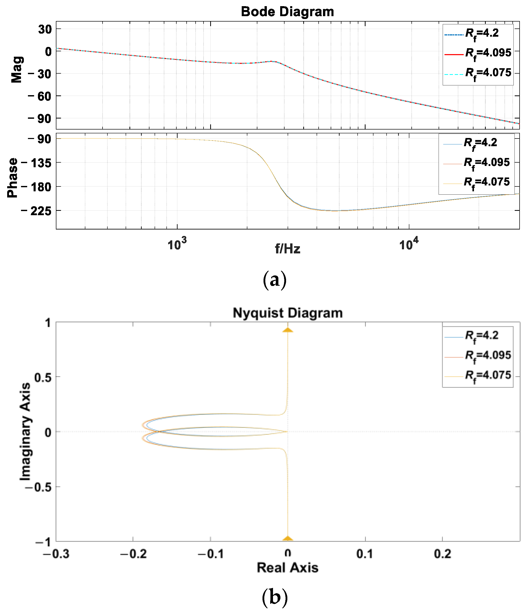
4.1. Stability Analysis Based on Linearized Switching Model

To keep consistency with the simulations in Section 3.2, the same values specified in Table 1 are used. According to Equation (7), the bode plot and Nyquist curve under different conditions can be found in Figure 10 and Figure 11, respectively.

When the damping resistance R_f = 4.3 Ω, the analysis results are as shown in Figure 10 as k_p varies. It can be seen in Figure 10a that the phase curve does not intersect with the −180 point when the amplitude curve gain is higher than 0 dB, which means that the system keeps stable as k_p varies. There is also no open-loop right half-plane pole, as shown in Figure 11b. According to the Nyquist stability criterion, the outputs under different conditions are all shown to be stable.

When the proportional coefficient k_p = 4.5, the analysis results are as shown in Figure 11 as R_f varies. From Figure 11, it is easy to obtain the same conclusion that the system does not lose its stability under these conditions, which is inconsistent with the simulations in Section 3.2, indicating that the stability analysis method based on the linearized switching model is not suitable to study the oscillations in simulations presented in Section 3.2. The reason is that the nonlinear characteristics in electronics may be ignored with the linearized switching model.

4.2. Stability Analysis Based on Nonlinear Dynamics

4.2.1. Average Model of the Circuit

According to Equation (3), the average equation of the single-phase voltage source full-bridge inverter circuit with an LCL filter is obtained as follows:

$$\left\{\begin{array}{l}{\displaystyle \frac{\mathrm{d}〈u_c〉}{\mathrm{d}t}}={\displaystyle \frac{1}{C}}〈i_1〉-{\displaystyle \frac{1}{C}}〈i_2〉\hfill \\ {\displaystyle \frac{\mathrm{d}〈i_1〉}{\mathrm{d}t}}=-{\displaystyle \frac{1}{L_1}}〈u_C〉-{\displaystyle \frac{R_f}{L_1}}〈i_1〉+{\displaystyle \frac{R_f}{L_1}}〈i_2〉+{\displaystyle \frac{(2D-1)E}{L_1}}\hfill \\ {\displaystyle \frac{\mathrm{d}〈i_2〉}{\mathrm{d}t}}={\displaystyle \frac{1}{L_2}}〈u_C〉+{\displaystyle \frac{R_f}{L_2}}〈i_1〉-{\displaystyle \frac{R_f+R}{L_2}}〈i_2〉\hfill \end{array}\right.$$

(8)

where $〈u_C〉$ is the state variable, u_c is the average value in a switching period, $〈i_1〉$ is the average value of the state variable in a switching period, $〈i_2〉$ is the average value of state variable i₂ in a switching period, and D is the duty cycle.

According to the modulation strategy as mentioned in Section 2.1, the relationship between the duty cycle and the control signal can be obtained as follows:

$$D(t)={\displaystyle \frac{1}{2}}(1+{\displaystyle \frac{〈i_{con}〉}{V_{tri}}})$$

(9)

4.2.2. Hopf Bifurcation Analysis

The state variable X_e is defined as the equilibrium point of the circuit, and the eigenvalue of the Jacobian matrix corresponding to the equilibrium point can be used to judge the stability of the circuit. According to Equation (9), the Jacobian matrix of the circuit near the equilibrium point X_e is obtained as follows:

$$J\left(X_e\right)=\left[\begin{array}{ccc}0& {\displaystyle \frac{1}{C}}& -{\displaystyle \frac{1}{C}}\\ -{\displaystyle \frac{1}{L_1}}& -{\displaystyle \frac{R_{\mathrm{f}}}{L_1}}& {\displaystyle \frac{R_{\mathrm{f}}-k_{\mathrm{p}}E}{L_1}}\\ {\displaystyle \frac{1}{L_2}}& {\displaystyle \frac{R_f}{L_2}}& -{\displaystyle \frac{R_{\mathrm{f}}+R}{L_2}}\end{array}\right]$$

(10)

From Equation (10), the characteristic polynomial of the Jacobian matrix is as follows:

$$F_1{\lambda }^3+F_2{\lambda }^2+F_3\lambda +F_4=0$$

(11)

where $F_1=1$, $F_2={\displaystyle \frac{R_{\mathrm{f}}}{L_1}}+{\displaystyle \frac{R}{L_2}}+{\displaystyle \frac{R_{\mathrm{f}}}{L_2}}$, $F_3={\displaystyle \frac{k_{p}E{R}_{\mathrm{f}}}{L_1{L}_2}}+{\displaystyle \frac{R{R}_{\mathrm{f}}}{L_1{L}_2}}+{\displaystyle \frac{1}{L_{1}C}}+{\displaystyle \frac{1}{L_{2}C}}$, and $F_4={\displaystyle \frac{k_{p}E+R}{L_1{L}_{2}C}}$.

The same circuit parameters as those in the PSIM simulation are used. For R_f = 4.3 Ω, the eigenvalue λ is calculated according to Equation (11), as shown in

Table 3. Solutions for λ as k_p increases.

kp	Characteristic Root	System Status
4.2	−313.8650 ± 1.8214 × 104i, −9.8667 × 103	equilibrium point
4.3	−247.3777 ± 1.8288 × 104i, −9.9997 × 103	equilibrium point
4.4	−182.1180 ± 1.8363 × 104i, −1.0130 × 103	equilibrium point
4.5	−118.0462 ± 1.8436 × 104i, −1.0258 × 103	equilibrium point
4.6891	0.00027 ± 1.8576 × 104i, −1.0494 × 103	Hopf bifurcation
4.76	43.2502 ± 1.8627 × 104i, −1.0581 × 103	unstable

. It can be seen that the system loses the stable state and undergoes slow-scale Hopf bifurcation with the increase in k_p. For k_p = 4.5, the calculated eigenvalues as R_f vary according to Equation (11) and are shown in

Table 4. Solutions for λ as R_f decreases.

Rf	Characteristic Root	System Status
4.4	−185.7460 ± 1.8443 × 104, −1.0251 × 104	equilibrium point
4.3	−118.0462 ± 1.8436 × 104i, −1.0258 × 104	equilibrium point
4.2	−50.3659 ± 1.8430 × 104i, −1.0266 × 104	equilibrium point
4.1	−16.5331 ± 1.8427 × 104i, −1.0270 × 104	equilibrium point
4.12556	0.0027 ± 1.8425 × 104i, −1.0272 × 104	Hopf bifurcation
4.09	24.0600 ± 1.8423 × 104i, −1.0274 × 104	unstable

. It can be found that the system loses its stable state and Hopf bifurcation occurs with the decrease in R_f.

In short, the theoretical analysis results are consistent with the simulations presented in Section 3.2. Compared with the analysis method based on the linearized switching model, the method based on the nonlinear dynamics is more accurate for the oscillation analysis in this situation.

Based on Equation (8), the analytical stability boundary of the system can be derived according to the Shengjin formula and the stability judgment, as shown in Equation (12). Once the following condition is met, the system is stable.

$$F_2>{\displaystyle \frac{1}{2}}\left(\sqrt[3]{Y_1}+\sqrt{Y_2}\right)$$

(12)

where

$$Y_1=\left(F_2^2-3F_1{F}_3\right)F_2+3F_3{\displaystyle \frac{9F_1{F}_4-F_2{F}_3+\sqrt{{\left(9F_3{F}_4-F_2{F}_3\right)}^2-4\left(F_2^2-3F_1{F}_3\right)\left(F_3^2-3F_2{F}_4\right)}}{2}}, \mathrm{and}$$

$$Y_2=\left(F_2^1-3F_1{F}_3\right)F_2+3F_1{\displaystyle \frac{9F_1{F}_4-F_2{F}_3-\sqrt{{\left(9F_1{F}_4-F_2{F}_3\right)}^2-4\left(F_2^2-3F_1{F}_1\right)\left(F_3^2-3F_2{F}_4\right)}}{2}}$$

According to Equation (12), the stable boundary of the single-phase voltage source inverter with LCL filter on the k_p-R_f plane is drawn compared with the stable boundary of PSIM simulation and the traditional design methods, which are shown in Figure 12, while the key data of the stability boundary are presented in

Table 5. Key data of the stability boundary.

Rf	Traditional Method/Rf′	Simulation Results/kp	Theoretical Results/kp
2.3 Ω	4.3 Ω	2.91	2.92
2.8 Ω	4.3 Ω	3.29	3.29
3.3 Ω	4.3 Ω	3.71	3.72
3.8 Ω	4.3 Ω	4.18	4.17
4.3 Ω	4.3 Ω	4.75	4.72
4.8 Ω	4.3 Ω	5.34	5.39
5.3 Ω	4.3 Ω	6.05	5.97
1.3 Ω	4.3 Ω	2.24	2.28

.

Obviously, Figure 12 shows that the boundaries obtained analytically using Equation (12) match the simulation results but are inconsistent with the traditional damping resistance design method. It can be seen that slow-scale instability can still appear in the traditional stable region because the traditional damping resistance design method has limitations in that it is based on the transmission characteristics and power loss of the filter without considering the influence of the controller on the system stability. The data in Table 5 quantitatively illustrate the consistency between simulation results and theoretical analysis. According to Equation (1), the traditional design method of R_f is relevant to the resonant frequency and capacitance value of the LCL filter without taking the effect of the controller parameter into account that the boundary keeps constant.

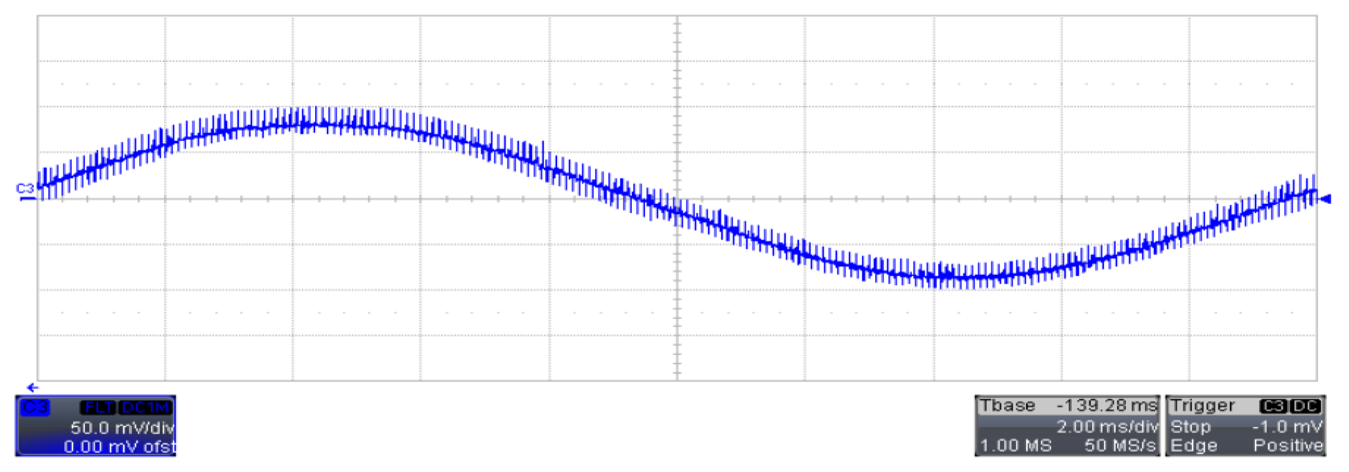
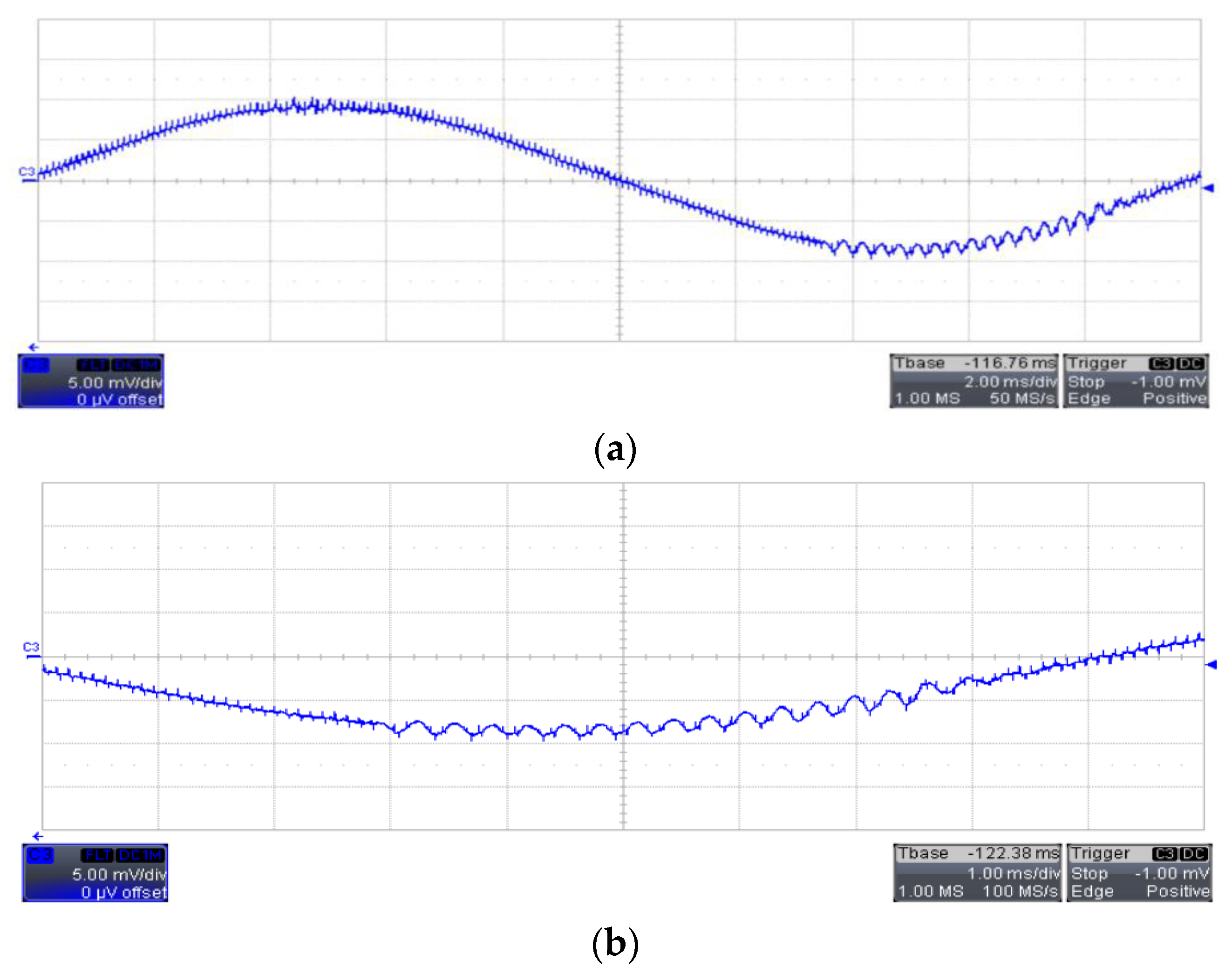
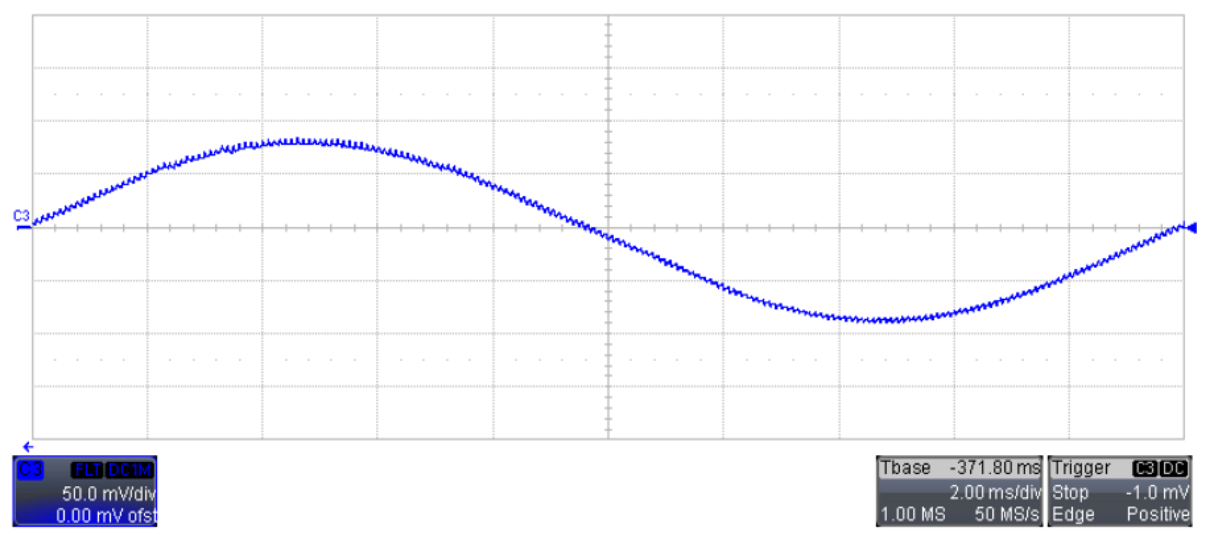
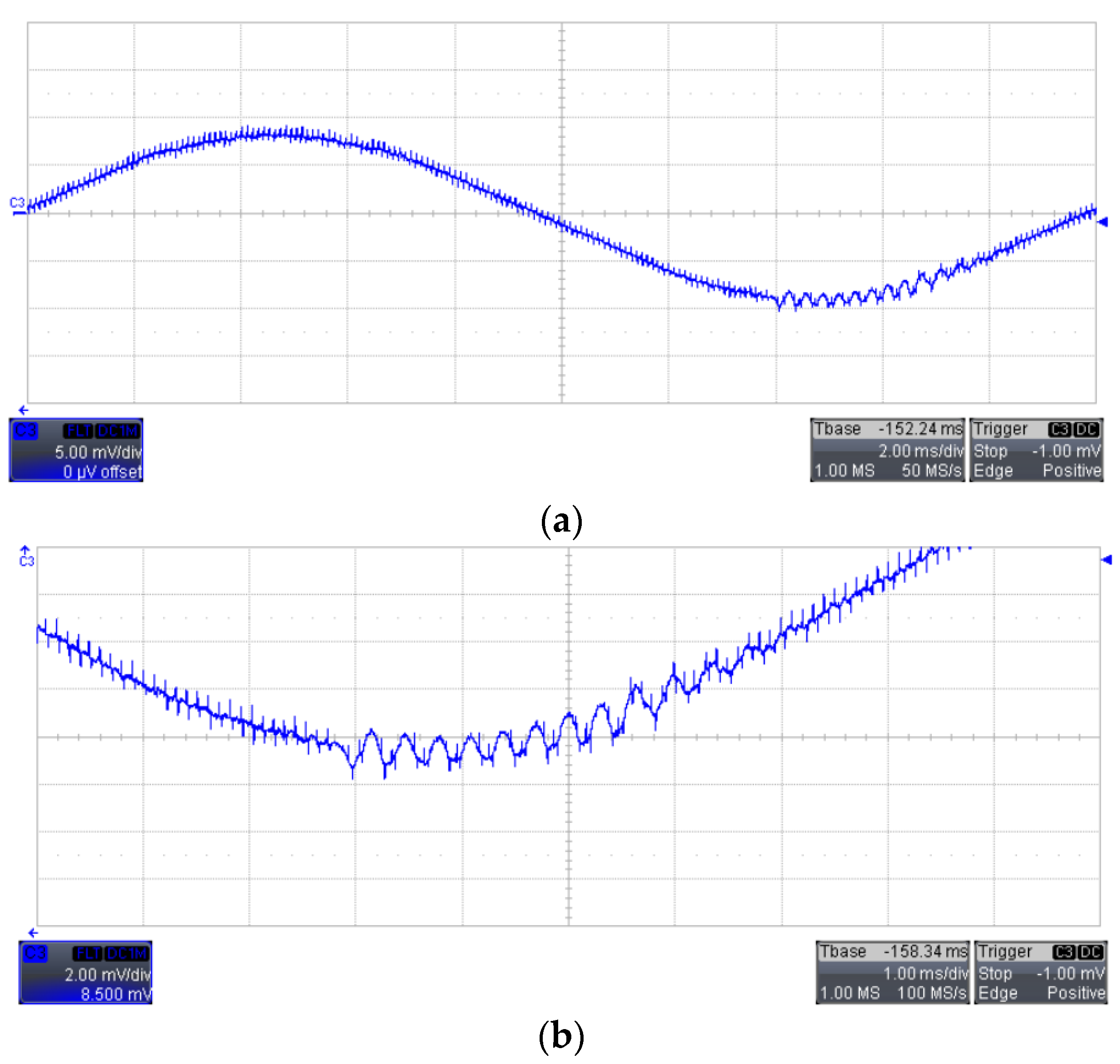
5. Experimental Verification

In order to verify the observed slow-scale bifurcation and the theoretical analysis above, an experimental circuit of a single-phase full-bridge voltage source inverter with an LCL filter is built, and the same circuit parameters in simulations shown in Section 3 are adopted. The experimental schematic diagram, which contains the main circuit, drive circuit, time delay circuit, and control circuit, is shown in Figure 13, in which the power switch and the driver are IRF540 (minos, Shenzhen, China) and IR2110 (Infineon, Munich, Germany), respectively. In addition, a Teledyne LeCroy oscilloscope (Teledyne LeCroy, New York, NY, USA) and Tektronix A622 current probe (Tektronix, Johnston, IA, USA) are used to capture the measured waveforms.

5.1. k_p as the Bifurcation Parameter

With the damping resistance R_f = 4.3 Ω, k_p is taken as the bifurcation parameter. Figure 14 shows the time domain waveform of inductor current i₂ for k_p = 4.5. It can be seen that the current waveform is smooth and the peak value is 1A, indicating that the system is operating in a steady state.

When k_p increases to 5.58, the time domain waveform of inductor current i₂ is shown in Figure 15. It can be seen that the time domain waveform of i₂ begins to oscillate at a low frequency and the oscillation frequency is about 3.2 kHz, which is generally in agreement with the simulation results and theoretical analysis. The discrepancies can be attributed to the introduced sample resistance and the parasitic parameters in the experiment.

5.2. R_f as the Bifurcation Parameter

With the proportional coefficient k_p = 4.5, R_f is taken as the bifurcation parameter. When the damping resistance R_f = 4.2 Ω, the time domain waveform of the inductor current i₂ is shown in Figure 16. From the time domain waveforms of the inductor current i₂, it can be seen that the system works in a stable state.

When R_f reduces to 3.3 Ω, the time domain waveform of the inductor current i₂ and its closed-up view are shown in Figure 17. It can be seen that the time domain waveform of the inductor current i₂ oscillates at a low frequency of about 3 kHz. Comparing the results of the simulations, theoretical analyses, and experiments, it can be concluded that they are in generally agreement with each other.

By comparison, it can be found that the system can still operate stably when the damping resistance is less than the traditional design standard. It is clear that the derived analytical expression of the stability boundary extends the selection range of damping resistance R_f in engineering design.

6. Conclusions

The slow-scale oscillation corresponding to Hopf bifurcation is investigated according to the characteristic polynomial of the Jacobian matrix, which is derived from the averaged model of the circuit, and the intrinsic mechanism of the instability of the voltage-controlled full-bridge inverter with an LCL filter is obtained using the nonlinear dynamics method. Moreover, the analytical stability boundary has been deduced based on the proposed theoretical analysis method, which will facilitate the selection of the appropriate parameter values to protect the system from instability in practice and expand the selection range of damping resistance compared with the traditional method. The experimental results demonstrate that the deduced analytical stability boundary of the inverter is able to predict the slow-scale instability within an acceptable range of error for practical applications.

This research contributes to the stability study of a voltage-controlled full-bridge inverter with an LCL filter using the nonlinear dynamics method, and the results greatly promote the understanding of complex behaviors in power electronic systems, revealing the characteristics and mechanisms of nonlinear phenomena. Furthermore, the analytical stability boundary deduced can improve the design of the system in practice.

References

1. Bughneda, A.; Salem, M.; Richelli, A.; Ishak, D.; Alatai, S. Review of Multilevel Inverters for PV Energy System Applications. Energies 2021, 14, 1585. [Google Scholar] [CrossRef]
2. Cai, Y.; He, Y.; Zhou, H.; Liu, J. Active-Damping Disturbance-Rejection Control Strategy of LCL Grid-Connected Inverter Based on Inverter-Side-Current Feedback. IEEE J. Emerg. Sel. Top. Power Electron. 2021, 9, 7183–7198. [Google Scholar]
3. Singh, J.K.; Prakash, S.; Al Jaafari, K.; Al Zaabi, O.; Al Hosani, K.; Behera, R.K.; Muduli, U.R. Active Disturbance Rejection Control of Photovoltaic Three-Phase Grid Following Inverters Under Uncertainty and Grid Voltage Variations. IEEE Trans. Power Delivery 2023, 38, 3155–3168. [Google Scholar]
4. Ma, G.D.; Xie, C.; Li, C.; Zou, J.X.; Guerrero, J.M. Passivity-Based Design of Passive Damping for LCL-Type Grid-Connected Inverters to Achieve Full-Frequency Passive Output Admittance. IEEE Trans. Power Electron. 2023, 38, 16048–16060. [Google Scholar]
5. Ye, J.; Wang, H.Z.; Li, B.J.; Huang, Y.K.; Xu, J.B.; Shen, A.W. Passivity-Based Controller Design of PCC Voltage Feedforward Active Damping for Grid-Connected Inverters. IEEE Trans. Ind. Electron. 2023, 38, 16048–16060. [Google Scholar]
6. Zhe, W.; Ishak, D.; Hamidi, M.N. A Grid-Connected Inverter with Grid-Voltage-Weighted Feedforward Control Based on the Quasi-Proportional Resonance Controller for Suppressing Grid Voltage Disturbances. Energies 2024, 17, 885. [Google Scholar] [CrossRef]
7. Zhang, J.S.; Yang, X.; Chen, W.J.; Zhou, H.W.; Luo, J. A Multifrequency Small-Signal Model for the MLCL-Filtered Grid-Connected Inverter Considering the FCE of Nonlinear Inductors. IEEE Trans. Ind. Electron. 2023, 70, 4901–4911. [Google Scholar]
8. Zhang, R.; Zhang, C.H.; Xing, X.Y.; Chi, S.M.; Liu, C.; Fang, J.Y. Modeling and Attenuation of Common Mode Resonance Current for Improved LCL-Type Parallel Inverters in PV Plants. IEEE Trans. Ind. Inform. 2023, 20, 5193–5205. [Google Scholar] [CrossRef]
9. Han, Y.; Mengling, Y.; Li, H.; Yang, P.; Xu, L.; Coelho, E.A.; Guerrero, J.M. Modeling and Stability Analysis of LCL -Type Grid-Connected Inverters: A Comprehensive Overview. IEEE Access 2019, 7, 114975–115001. [Google Scholar]
10. Pea-Alzola, R.; Liserre, M.; Blaabjerg, F.; Sebastián, R.; Dannehl, J.; Fuchs, F.W. Analysis of the passive damping losses in LCL-filter based grid converters. IEEE Trans. Power Electron. 2013, 28, 2642–2646. [Google Scholar]
11. Wu, W.; Liu, J.; Li, Y.; Blaabjerg, F. Individual Channel Design-Based Precise Analysis and Design for Three-Phase Grid-Tied Inverter With LCL-Filter Under Unbalanced Grid Impedance. IEEE Trans. Power Electron. 2020, 35, 5381–5396. [Google Scholar]
12. Khan, D.; Qais, M.; Hu, P. A reinforcement learning-based control system for higher resonance frequency conditions of grid-integrated LCL-filtered BESS. J. Energy Storage 2024, 93, 112373. [Google Scholar]
13. Yang, Z.; Shah, C.; Chen, T.; Yu, L.; Joebges, P.; De Doncker, R.W. Stability Investigation of Three-Phase Grid-Tied PV Inverter Systems Using Impedance Models. IEEE J. Emerg. Sel. Top. Power Electron. 2022, 10, 2672–2684. [Google Scholar]
14. Li, X.Q.; Wu, X.J.; Geng, Y.W.; Zhang, Q. Stability Analysis of Grid-Connected Inverters with an LCL Filter Considering Grid Impedance. J. Power Electron. 2013, 13, 896–908. [Google Scholar]
15. Zhu, T.; Huang, G.; Ouyang, X.; Zhang, W.; Wang, Y.; Ye, X.; Wang, Y.; Gao, S. Analysis and Suppression of Harmonic Resonance in Photovoltaic Grid-Connected Systems. Energies 2024, 17, 1218. [Google Scholar] [CrossRef]
16. Yang, J.X.; Tse, C.K.; Liu, D. Sub-Synchronous Oscillations and Transient Stability of Islanded Microgrid. IEEE Trans. Power Syst. 2023, 38, 3760–3774. [Google Scholar]
17. Cao, H.B.; Wang, F.Q.; Liu, J.J. Analysis of Fast-Scale Instability in Three-Level T-Type Single-Phase Inverter Feeding Diode-Bridge Rectifier With Inductive Load. IEEE Trans Power Electron. 2022, 37, 15066–15083. [Google Scholar]
18. Luo, C.; Liu, T.; Wang, X.F.; Ma, X.K. Design-Oriented Analysis of DC-Link Voltage Control for Transient Stability of Grid-Forming Inverters. IEEE Trans. Ind. Electron. 2024, 71, 3698–3707. [Google Scholar]
19. Yang, F.; Yang, L.H.; Ma, X.K. Fast-Scale Bifurcation Analysis in One-Cycle Controlled H-Bridge Inverter. Int. J. Bifurcat. Chaos 2016, 26, 1650199. [Google Scholar]
20. Cheng, C.; Xie, S.; Qian, Q.; Xu, J. On Absolute Stability of Open-Loop Synchronized Single-Phase Grid-Following Inverters. IEEE Trans. Ind. Electron. 2023, 70, 10239–10248. [Google Scholar]
21. Cheng, C.; Xie, S.; Xu, J.; Qian, Q. Universal Absolute Stability Criterion for Single-Phase Grid-Following Inverters Equipped With Orthogonal-Normalization-Based Grid Synchronizer. IEEE Trans. Power Electron. 2023, 38, 9090–9099. [Google Scholar]
22. Avrutin, V.; Zhusubaliyev, Z.T.; Suissa, D.; El Aroudi, A. Non-observable chaos in piecewise smooth systems. Nonlinear Dyn. 2020, 99, 2031–2048. [Google Scholar]
23. Zhusubaliyev, Z.T.; Avrutin, V.; Kucherov, A.S.; Haroun, R.; El Aroudi, A. Period adding with symmetry breaking/recovering in a power inverter with hysteresis control. Physica D 2023, 444, 133600. [Google Scholar]
24. Yin, Z.; Gong, R.; Lu, Y. Slow-Scale Nonlinear Control of a H-Bridge Photovoltaic Inverter. Electronics 2023, 12, 2000. [Google Scholar] [CrossRef]
25. Keyvani-Boroujeni, B.; Shahgholian, G.; Fani, B. A Distributed Secondary Control Approach for Inverter Dominated Microgrids with Application to Avoiding Bifurcation Triggered Instabilities. IEEE J. Emerg. Sel. Top. Power Electron. 2020, 8, 3361–3371. [Google Scholar]
26. Ji, H.; Xie, F.; Shen, L.; Yang, R.; Zhang, B. Unstable behavior analysis and stabilization of double-loop proportional-integral control H-bridge inverter with inductive impedance load. Int. J. Circuit Theory Appl. 2022, 50, 904–925. [Google Scholar]
27. Lei, B.; Xiao, G.C.; Wu, X.L.; Zheng, L. A unified “scalar” discrete-time model for enhancing bifurcation prediction in digitally controlled H-bridge grid-connected inverter. Int. J. Bifurcat. Chaos 2013, 23, 1350126. [Google Scholar]
Figure 1. Schematic diagram of single-phase voltage source full-bridge inverter with LCL filter.
Energies 17 04168 g001
Figure 2. Linearized switching model of single-phase voltage source full-bridge inverter with LCL filter.
Energies 17 04168 g002
Figure 3. The inductor current with a 50 percent increase in reference current.
Energies 17 04168 g003
Figure 4. Simulation results for kp = 4.5 (a) time domain waveform of i2 (b) FFT.
Energies 17 04168 g004
Figure 5. Simulation results for kp = 4.72 (a) time domain waveform of i2 (b) FFT.
Energies 17 04168 g005
Figure 6. Simulation results for kp = 4.74 (a) time domain waveform of i2 (b) FFT.
Energies 17 04168 g006
Figure 7. Simulation results for Rf = 4.2 Ω (a) time domain waveform of i2 (b) FFT.
Energies 17 04168 g007
Figure 8. Simulation results for Rf = 4.095 (a) time domain waveform of i2 (b) FFT.
Energies 17 04168 g008
Figure 9. Simulation results when Rf = 4.075 (a) time domain waveform of i2 (b) FFT.
Energies 17 04168 g009
Figure 10. (a) Frequency response (b) Nyquist curve when Rf = 4.3.
Energies 17 04168 g010
Figure 11. (a) Frequency response (b) Nyquist curve when Rf = 4.5.
Energies 17 04168 g011
Figure 12. Comparison of the theoretical analysis, the simulation, and traditional design methods.
Energies 17 04168 g012
Figure 13. Experimental schematic diagram of the voltage source full-bridge inverter with LCL filter.
Energies 17 04168 g013
Figure 14. Inductor current waveform when Rf = 4.3 Ω, kp = 4.5.
Energies 17 04168 g014
Figure 15. Current waveform of i2 for Rf = 4.3 Ω, kp = 5.58 (a) time domain waveform of i2 (b) closed up view of i2.
Energies 17 04168 g015
Figure 16. Current waveform of i2 for kp = 4.5, Rf = 4.2 Ω.
Energies 17 04168 g016
Figure 17. Current waveform of i2 for kp = 4.5, Rf = 4.2 Ω (a) time domain waveforms of i2 (b) close-up view of i2.
Energies 17 04168 g017