Optimal Operation of a Novel Small-Scale Power-to-Ammonia Cycle under Possible Disturbances and Fluctuations in Electricity Prices

Abstract

Power-to-Ammonia (P2A) is a promising technology that can provide a low-emission energy carrier for long-term storage. This study presents an optimization approach to a novel small-scale containerized P2A concept commissioned in 2024. A dynamic nonlinear optimization problem of the P2A concept is set up, employing the non-commercial MOSAIC^® software V3.0.1 in combination with the NEOS^® server. In total, seven optimization solvers, ANTIGONE^®, CONOPT^®, IPOPT^®, KNITRO^®, MINOS^®, PATHNLP^®, and SNOPT^®, are used. The first and main part of this work optimizes several disturbance scenarios of the concept and aims to determine the optimal reactor temperature profile to counter the disturbances. The optimization results suggest, for example, lowering the reactor temperature profile if the hydrogen and nitrogen inlet streams into the system decrease. The second part of this work presents a crude dynamic optimal scheduling model. This part aims to determine the amount of ammonia to be produced and sold given a randomized price of electricity for three consecutive points in time. The optimization results recommend decreasing production when the price of electricity is high and vice versa. However, the dynamic model must be improved to include fluctuations in the price of ammonia. Then, it can be used as a real-time optimization tool.

1. Introduction

The threat of climate change looms. For example, between 1993 and 2023, sea levels rose by 10 cm [1]. In 2100, 410 million people, i.e., 4% of the world population of 10.4 billion [2], are expected to be affected by coastal flooding [3]. This calls for rigorous greenhouse gas control and the replacement of fossil fuels with cleaner energy carriers like hydrogen.

In Europe [4], including Germany [5,6], and worldwide [7], hydrogen produced via water electrolysis powered by renewable electricity is seen as a promising carbon-free energy vector. However, hydrogen derivatives like ammonia might be a preferred solution for transportation and long-term storage. To have the same energy content as marine diesel, ammonia only requires a tank size that is three times larger under comparatively mild conditions, i.e., 25 °C and 10 bar. In contrast, hydrogen requires a tank size that is four times larger at much harsher conditions of −253 °C and 1.01325 bar [8,9].

Low-emission ammonia as an energy vector and long-term hydrogen carrier is being increasingly discussed and implemented. For example, Germany has struck trade agreements with Canada [10,11] and Egypt [12] to import low-emission ammonia. However, as of now, ammonia production is one of the biggest carbon-emitting chemical processes and contributes to 1% of global greenhouse gas (GHG) emissions. Overall, ammonia accounts for 2% of the total world energy consumption [13,14].

Traditionally, ammonia (NH₃) is produced continuously on a large scale from fossil fuels, mainly natural gas or coal, along with water as the source of hydrogen (H₂) and air as the source of nitrogen (N₂), through the Haber–Bosch process. This process is a gaseous heterogeneous exothermic catalytic equilibrium reaction that takes place at 100–350 bar and 400–550 °C, as shown in Equation (1). Currently, daily plant capacities reach up to 3300 tons, producing about 1.33 t of carbon dioxide per ton of ammonia [15,16,17,18,19].

$$1.5{\mathrm{H}}_{2\left(\mathrm{g}\right)}+0.5{\mathrm{N}}_{2\left(\mathrm{g}\right)}\rightleftharpoons {\mathrm{NH}}_{3\left(\mathrm{g}\right)} ;\Delta {\overline{h}}^{°}=-46.22 \mathrm{kJ}/{\mathrm{mol}}_{{\mathrm{NH}}_3}$$

(1)

On the other hand, low-emission ammonia production, so-called Power-to-Ammonia (P2A), uses renewable electricity to power water electrolysis and air-separation units to yield hydrogen and nitrogen [20]. The challenge hereby lies in the nature of the renewable energy sources, i.e., their intermittency. Because of this, the price of electricity can also fluctuate. This means that P2A not only has to be flexible in terms of the availability of electricity, but also must account for its cost.

Compared to large-scale P2A, small-scale P2A is more advantageous due to its flexibility [21]. The reactor’s start-up time is much shorter. In addition, the need to store hydrogen as a buffer is lower [22]. Small-scale P2A could be used by farmers in remote locations to produce their own ammonia, which could be used both as tractor fuel and as fertilizer [23,24,25,26].

One such small-scale P2A system has been developed in the European Union’s FLEXnCONFU project (Flexibilize combined cycle power plant through power-to-X solutions using non-conventional fuels) [27,28]. In the project, a novel containerized P2A concept was designed to ensure maximum operation load flexibility, i.e., a fast dynamic behaviour. The P2A container is depicted in Figure 1. The project started in April 2020, and the first tests are scheduled for the end of 2024 at the University of Genova, Savona Campus, Italy. Prospectively, the P2A container will be incorporated into the existing micro heating, cooling, and electricity grid of the campus, which includes a retrofitted micro gas turbine that runs on ammonia. Using this process, the full Power-to-Ammonia-to-Power (P2A2P) chain will be tested.

In this work, we present an optimization approach to the novel concept, which is based on the freeware MOSAIC^® and makes use of the NEOS^® server. The optimization approach is split into two parts. In the first and main part, we determine the optimal temperature profile of the reactor, which can counteract seven disturbance scenarios that can occur during operation. Thus, the first part provides the plant operators with the right countermeasures should these small disturbances occur.

The second part of this work presents the dynamic optimization of the novel P2A concept. The price of electricity is randomized in three consecutive time steps. The optimization approach determines the amount of ammonia to be produced and sold to maximize profits given restrictions regarding the ammonia storage capacity. This dynamic optimization model shall, in the long run, act as a real-time optimization tool to determine the optimal plant operation given day-ahead electricity prices.

2. Power-to-Ammonia Optimization Background

Process modelling requires the choice of suitable simulation and optimization software. For ammonia production applications, several different approaches can be found in the recent literature.

For example, Flórez-Orrego and de Oliveira Junior [29] used the software Aspen HYSYS^® V8.6 [30]. They implemented user-defined functions to minimize the total exergy destruction of a conventional methane-reforming ammonia production unit of 1000 t/d. The optimization problem was of the nonlinear type (NLP), for which the inbuilt sequential quadratic programming (SQP) tool of Aspen HYSYS^® was used.

Demirhan et al. [31] used the optimization environment GAMS^® V24.4.5 [32,33,34] on different ammonia production pathways using renewables, biomass, or natural gas as feedstock, producing up to 1000 t/d. Each pathway results in a mixed integer nonlinear optimization problem (MINLP). The integers result from the fact that each pathway can consist of various unit operations. An adapted branch and bound (B&B) algorithm was applied to minimize the levelized cost of ammonia production.

Matos et al. [35] implemented a system of ordinary differential equations (ODEs) in MATLAB^® [36] to emulate the behaviour of an ammonia synthesis reactor. The optimization of the nitrogen conversion and economic return was implemented in non-derivative direct search iteration routines, where the ODE was solved using the Runge–Kutta method. The optimizing variables were the reactor inlet gas temperature and nitrogen flow, as well as the reactor temperature and length.

Table 1 summarizes and compares the above-mentioned and more recent studies from the literature on ammonia optimization approaches. This work’s approach is listed in the last line of Table 1. As can be seen in Table 1, the variety of optimization software used is large. However, all of the software is commercial, except for JuMP^® employed by Andrés-Martínez et al. and the MOSAIC^®-NEOS^® approach in this work. The problem formulation is performed either internally by the software or by hand. For seven out of the twelve works presented in Table 1, the problem formulation was performed by hand. This is also true for the MOSAIC^®-NEOS^® approach. Formulating a problem by hand is time-consuming. However, it provides the freedom to fully describe a problem and adjust the equations to a special case.

Depending on the type of the problem, NLP, MINLP, etc., a suitable solver must be used. For example, Osman et al. employed GUROBI^® in their dynamic linear problem (DLP). All of the studies from the literature listed in Table 1 employed a single solver to solve their optimization problems. Only this work employs more than one solver, i.e., the seven different solvers ANTIGONE^® [37], CONOPT^® [38], IPOPT^® [39], KNITRO^® [40], MINOS^® [41], PATHNLP^® [42], and SNOPT^® [43], as listed in Table 1 on the last line. This variety of solvers is the strength of the approach proposed here. Nonlinear problems often have local optimal solutions, and different solvers find different local solutions. However, if more than one solver is employed, the chance of finding the global optimum out of all the local optima is increased.

Table 1. An overview of ammonia-related optimization approaches in the literature.

Authors and Year	Ammonia Application	Ammonia Production	Software Employed	Problem Formulation	Problem Type	Optimization Solver or Approach	Objective Function
Flórez-Orrego and de Oliveira Junior [29], 2017	Methane-based ammonia production	1000 t/d	Aspen HYSYS® V8.6	Internally	NLP	Approach: SQP	Exergy destruction
Demirhan et al. [31], 2018	Natural gas, biomass-based ammonia production, and P2A	≤1000 t/d	GAMS® V24.4.5	By hand	MINLP	Approach: B&B	Levelized cost of ammonia
Matos et al. [35], 2020	Ammonia synthesis reactor	5 t/d (calculated from data provided)	MATLAB®	By hand	ODE	Approach: Iteration of Runge–Kutta and Derivative-Free Direct Search Method	Nitrogen conversion and economic return
Osman et al. [44], 2020	P2A	1840 t/d	Aspen Plus® [45] with Python® [46]	By hand	DLP	GUROBI® [47]	Levelized cost of ammonia
Wang et al. [48], 2020	P2A and nitric acid production	510–680 t/d	gPROMS® [49]	Internally	DNLP	Approach: SQP [50]	Cost of ammonia
Kelley et al. [51], 2021	P2A	11–13 t/d (calculated from data provided)	gPROMS® V1.3.1	Internally	DNLP	Not disclosed	Cost of electric power
Deng et al. [52], 2022	P2A	240 t/d (calculated from data provided)	UniSim® [53]	Internally	DNLP	Not disclosed	Energy consumption
Nozari et al. [54], 2022	Energy Hub (power, heat, hydrogen, and ammonia production from natural gas and P2A)	0.07 t/d (calculated from data provided)	GAMS®	By hand	DMILP	CPLEX® [55]	Exergy destruction and operating costs
Andrés-Martínez et al. [56], 2023	P2A	61.2 t/d (calculated from data provided)	JuMP® [57]	By hand	DNLP	Approach: time and space discretization and then IPOPT® [39]	Ammonia production
Wang et al. [58], 2023	P2A	10.8 t/d (calculated from data provided)	Not disclosed	By hand	DNLP under uncertainties	Approach: Markov Decision Process [59]	Profit
Kong et al. [60], 2023	Renewable microgrid (P2H2P and P2A2P)	2.2 t/d (calculated from data provided)	MATLAB Simulink® V2022a [61] with Pyomo® Python V3.9. [62]	Internally	DMILP	Not disclosed	Operating costs
This study	P2A	0.04 t/d	MOSAIC® V3.0.1 with NEOS®	By hand	NLP and DNLP	ANTIGONE®, CONOPT®, IPOPT®, KNITRO®, MINOS®, PATHNLP® and SNOPT®	Ammonia production and profit

Table 1. An overview of ammonia-related optimization approaches in the literature.

Authors and Year	Ammonia Application	Ammonia Production	Software Employed	Problem Formulation	Problem Type	Optimization Solver or Approach	Objective Function
Flórez-Orrego and de Oliveira Junior [29], 2017	Methane-based ammonia production	1000 t/d	Aspen HYSYS® V8.6	Internally	NLP	Approach: SQP	Exergy destruction
Demirhan et al. [31], 2018	Natural gas, biomass-based ammonia production, and P2A	≤1000 t/d	GAMS® V24.4.5	By hand	MINLP	Approach: B&B	Levelized cost of ammonia
Matos et al. [35], 2020	Ammonia synthesis reactor	5 t/d (calculated from data provided)	MATLAB®	By hand	ODE	Approach: Iteration of Runge–Kutta and Derivative-Free Direct Search Method	Nitrogen conversion and economic return
Osman et al. [44], 2020	P2A	1840 t/d	Aspen Plus® [45] with Python® [46]	By hand	DLP	GUROBI® [47]	Levelized cost of ammonia
Wang et al. [48], 2020	P2A and nitric acid production	510–680 t/d	gPROMS® [49]	Internally	DNLP	Approach: SQP [50]	Cost of ammonia
Kelley et al. [51], 2021	P2A	11–13 t/d (calculated from data provided)	gPROMS® V1.3.1	Internally	DNLP	Not disclosed	Cost of electric power
Deng et al. [52], 2022	P2A	240 t/d (calculated from data provided)	UniSim® [53]	Internally	DNLP	Not disclosed	Energy consumption
Nozari et al. [54], 2022	Energy Hub (power, heat, hydrogen, and ammonia production from natural gas and P2A)	0.07 t/d (calculated from data provided)	GAMS®	By hand	DMILP	CPLEX® [55]	Exergy destruction and operating costs
Andrés-Martínez et al. [56], 2023	P2A	61.2 t/d (calculated from data provided)	JuMP® [57]	By hand	DNLP	Approach: time and space discretization and then IPOPT® [39]	Ammonia production
Wang et al. [58], 2023	P2A	10.8 t/d (calculated from data provided)	Not disclosed	By hand	DNLP under uncertainties	Approach: Markov Decision Process [59]	Profit
Kong et al. [60], 2023	Renewable microgrid (P2H2P and P2A2P)	2.2 t/d (calculated from data provided)	MATLAB Simulink® V2022a [61] with Pyomo® Python V3.9. [62]	Internally	DMILP	Not disclosed	Operating costs
This study	P2A	0.04 t/d	MOSAIC® V3.0.1 with NEOS®	By hand	NLP and DNLP	ANTIGONE®, CONOPT®, IPOPT®, KNITRO®, MINOS®, PATHNLP® and SNOPT®	Ammonia production and profit

Like the optimization software, many of the solvers used in the studies listed in Table 1 are commercial, e.g., GUROBI^® and CPLEX^®. Only IPOPT^® is non-commercial. Some of the solvers that are accessible through the NEOS^® server are also commercial. However, for research purposes, the solvers on NEOS^® can be used for free.

The non-commerciality, accessibility for the research community, freedom of problem formulation by hand, and solver variety make the MOSAIC^®-NEOS^® approach unique amongst the approaches used in the studies listed in Table 1.

3. Methods

This Section is divided into three subsections. In Section 3.1, the adopted MOSAIC^®-NEOS^® approach is explained. In Section 3.2, the novel P2A concept is described, to which the MOSAIC^®-NEOS^® approach is applied. Lastly, in Section 3.3, the two MOSAIC^®-NEOS^® optimization setups for the P2A concept are described. The results of these two setups are then presented in Section 4.

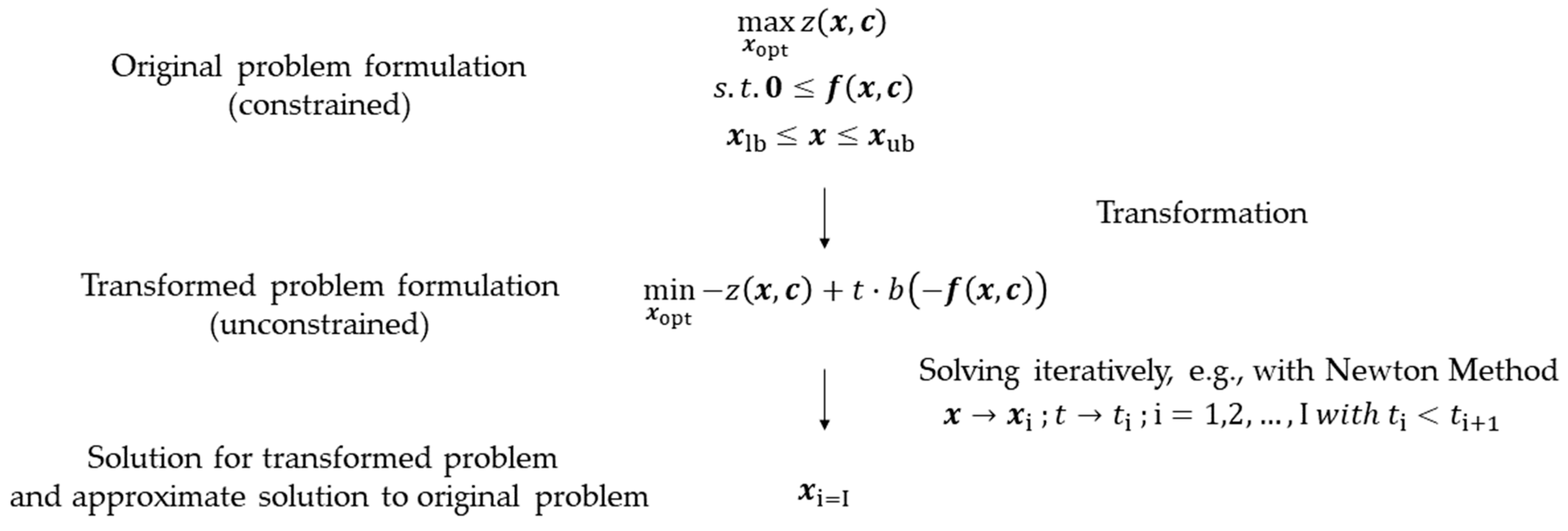
3.1. The MOSAIC^®-NEOS^® Optimization Approach

The characteristics of this work’s approach are given in the last line of Table 1. In this work, the software MOSAIC^® [63,64] and the NEOS Server^® [65,66,67] are employed in combination to solve an NLP and a DNLP of the proposed novel small-scale P2A cycle. The workflow of the MOSAIC^®-NEOS^® approach is schematically depicted in Figure 2.

MOSAIC^® is non-commercial and accessible to everyone in the research community. It allows for the relevant equations to be set up by hand using LaTeX^® script. The use of LaTeX^® script makes MOSAIC^® especially accessible to the scientific world, as LaTeX^® [68] is a widely used word and equation processing program. The created system of equations is translated using MOSAIC^® to optimization scripts like GAMS^®. The GAMS^® formulation of the problem is then sent to the NEOS^® server for solving. NEOS^® allows for the selection of multiple solvers. The solution of the optimization problem is then reimported into MOSAIC^®. Optionally, this result can be used as the initial solution for a follow-up optimization with, e.g., a different solver.

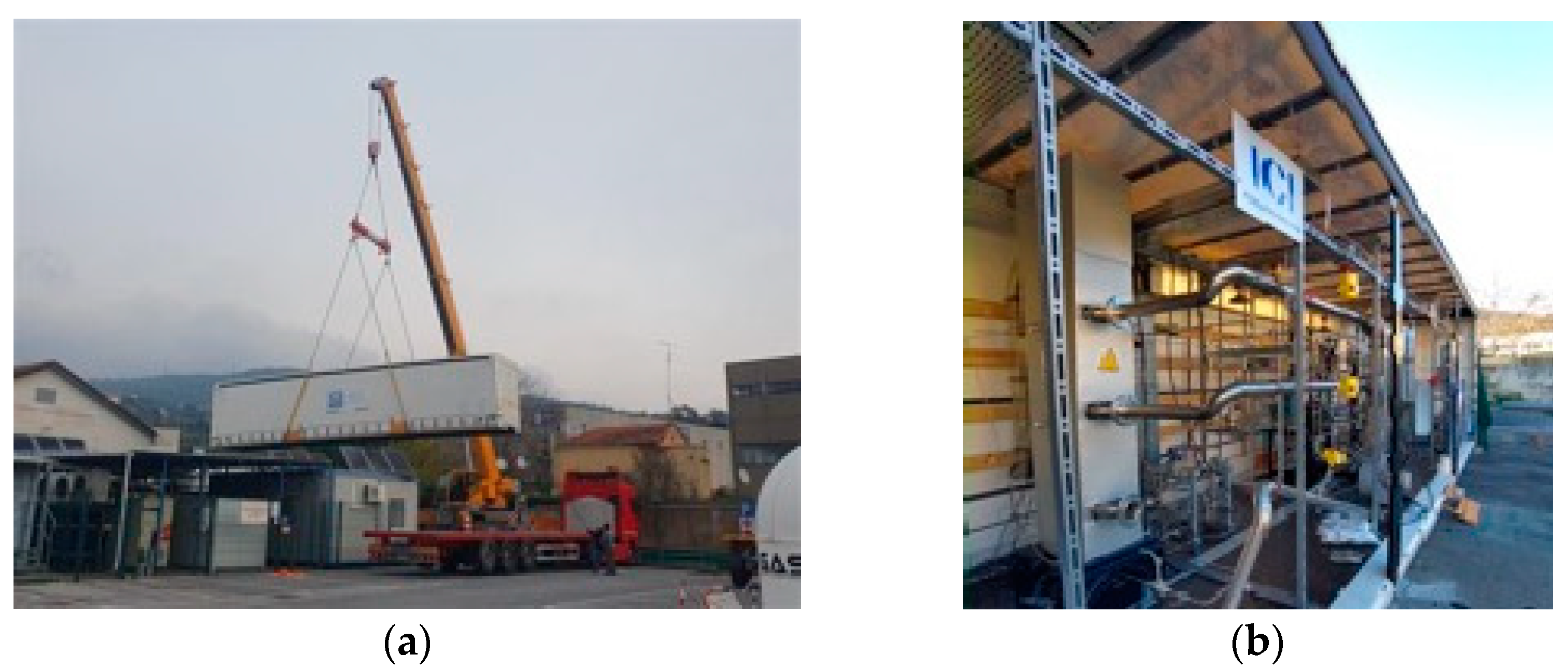
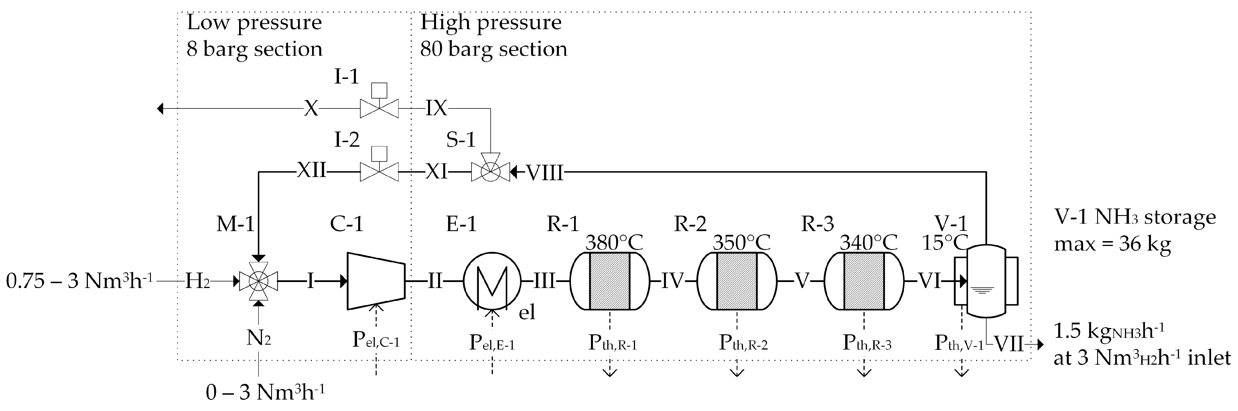
3.2. The FLEXnCONFU P2A System

The process diagram of the novel P2A process is given in Figure 3. H₂ and N₂ enter the system at 8 barg. The electrolyser capacity is between 0.75 and 3 Nm³H₂ h⁻¹. The N₂ is provided by bottles, and its inflow is controlled to match the H₂ influx for a molar ratio of 2.96 mole H₂ to 1 mole of N₂. The H₂ and N₂ are mixed with the recycled stream XII in the mixer M-1. Outlet stream I enters the electrically driven compressor C-1 to raise the pressure to 80 barg in outlet stream II. As depicted in Figure 3 by the dashed-line boxes, the novel process is divided into two pressure regimes: low pressure, 8 barg (imposed by the electrolyser outlet condition), and high pressure, 80 barg (set by the pressure targeted in the reactor).

Stream II enters the electric heater E-1 to heat up the reactor inlet III to the required synthesis temperature of 380 °C. The reactor is divided into three reaction bed sections, R-1, R-2, and R-3. Each of the three beds can be electrically heated or cooled via free and forced air convection. The optimal temperature profile of the sections is 380, 350, and 340 °C to maximize the thermal degree of efficiency of the cycle, as determined in a previous work [69]. The catalyst employed is a conventional iron-based one, but of the newest generation, which is envisioned to perform well at a much lower pressure and temperature than the industry standard of 100–350 bar and 400–550 °C. A new kinetic model fitted to test data from the catalyst supplier was implemented for the simulations (see again [69]).

In steady state and with the optimal profile from above, all three reactor sections need to be cooled due to the exothermic reaction. This is why the three heat streams P_th,R-1, P_th,R-2, and P_th,R-3 leave the system’s dotted boundary in Figure 3. Heat transfer calculations suggest that free convection is sufficient. The reactor product stream VI is cooled to 15 °C in separator V-1. Part of the NH₃ in stream VI condenses and leaves the system as the desired product in stream VII, which consists of 99 mol% NH₃. At maximum electrolyser production and a steady state, 1.5 kg h⁻¹ of NH₃ leaves the cycle via stream VII. The uncondensed NH₃ and unreacted H₂ and N₂ leave V-1 in the gaseous state in stream VIII, which is split in the splitter S-1. The very small stream IX is the purge stream to rid the system of undesired inerts. The much bigger stream XI enters the recycle valve I-2, which reduces the pressure back to 8 barg to equal the pressure of the cycle inlets.

The novelty of the process lies in three aspects, which are all meant to serve the cycle’s design for maximum flexibility and dynamic behaviour. First is the use of the electric heater E-1 instead of an internal gas–gas heat exchanger. The internal heat exchanger would make use of the thermal energy of the reactor outlet stream VI. The electric heater displays a faster dynamic behaviour without any feedback and instability concerns. Second, the low operating pressure and temperature regime also add to a faster start-up of the cycle. Third and last, the use of a recycle valve instead of a recycle compressor not only reduces the investment cost of the cycle, but also increases the speed of the start-up and load changes, since only the main compressor needs to be controlled.

For a deeper insight into the dynamic behaviour of the cycle, as well as how it compares exergetically and economically to a more conventional cycle, i.e., inferior in the first and superior in the latter case, the reader may refer to the previous works [70,71,72,73].

3.3. MOSAIC^®-NEOS^® Optimization Setups

A DNLP optimization problem can be formulated in the general form, as given in Equation (2):

$$\begin{gathered} \underset{{\mathit{x}}_{\mathrm{opt}}}{\max }z\left(\mathit{x},\mathit{c}\right) \\ \mathrm{such} \mathrm{that} \mathbf{0}\le \mathit{f}\left(\mathit{x},\mathit{c}\right) \\ {\mathit{x}}_{\mathrm{lb}}\le \mathit{x}\le {\mathit{x}}_{\mathrm{ub}} \end{gathered}$$

(2)

In Equation (2), $z$ is the objective function to be maximized, and $\mathit{f}$ is a vector of the constraint functions that need to be fulfilled. $z$ and $\mathit{f}$ are dependent on the vector of variables $\mathit{x}$ and a vector of constants, $\mathit{c}$. The variables are bound by lower and upper limits, expressed by the vectors ${\mathit{x}}_{\mathrm{lb}}$ and ${\mathit{x}}_{\mathrm{ub}}$. For Equation (2) to be the nonlinear and dynamic type, at least one of the functions needs to be nonlinear, and the variables are dependent on time, which means that each variable has one value for every point in time. The difference between an NLP and DNLP lies in the increased size of the problem. $\mathit{x}$ increases linearly with the number of time steps, while $\mathit{f}$ increases even more, depending on whether additional functions need to be implemented that connect the constraints from one time point to the next. $\mathit{x}$ itself contains the optimization and the dependent variables. The optimization variables ${\mathit{x}}_{\mathrm{opt}}$ are the free variables to be changed by the optimization solver in order to minimize $z$. The dependent variables ${\mathit{x}}_{\mathrm{dep}}$ are determined by the solution of the constraint vector $\mathit{f}$.

The DNLP formulation of this work consists of 871 equations and 880 variables, of which 9 are optimization variables. The number of time steps is three. Without the last two time steps and a different objective function, the DNLP reduces to an NLP of 289 equations and 292 variables, of which 3 are optimization variables.

There is a great variety in the approaches that optimization solvers take to solve a (D)NLP formulation. For example, the solver IPOPT^® employs an interior point method. The crude schematics of such an interior point approach are depicted in Figure 4. The original constrained problem formulation from Equation (2) is transformed into an unconstrained minimization problem. The transformed problem is an approximation of the original problem and is, in some cases, identical. The constraints $\mathit{f}$ still exist. They are incorporated into the boundary functions $b$, which are added to the objective function $\mathit{z}$. The boundary functions are multiplied with the penalty parameter $t$. The transformed problem is solved iteratively, e.g., with the Newton approach. In each iteration step i, the penalty parameter $t$ increases. The solution ${\mathit{x}}_{\mathrm{i}=\mathrm{I}}$ after I iterations is an approximate solution of the original problem. For the form of the boundary functions and the method to update the penalty parameter, several approaches exist [74].

To obtain an idea of the overall problem of this work, a selection of the equations describing the P2A concept, introduced in Section 3.2, is given in Table 2 and Table 3. In these tables, the equations for the first reactor segment R-1 and the condenser V-1 are presented. These equations all belong to the constraint vector $\mathit{f}$. Table 2 and Table 3 show that each unit operation is described by the corresponding mass (i.e., moles), energy, and entropy balances, as well as the pressure, temperature, and chemical equilibria equations. The mole balance equations in Table 2 include the numeric forward difference approach, which is applied to the reaction kinetics equations taken from previous work [74]. The kinetics are highly nonlinear, even though the simplest finite difference method was employed.

Table 2 also contains the polynomial equation of state equations for molar specific enthalpy and entropy taken from Barin and Knacke [75,76,77]. Their rather simple polynomial approach is only valid for ideal gaseous mixtures. In a previous exergetic analysis of the cycle [77], it could be shown that the assumption of an ideal gaseous mixture can be made.

The ammonia storage equation for V-1 in Table 3 means that the liquid ammonia leaving the cycle via stream VII is either sold or does not leave V-1, but is stored there in liquid form. Except for this equation, no other storage terms have been implemented. This is justified by the assumption that the thermal and mass storage capacities of unit operations in a small-scale system are negligible. This further implies that changes in operation points will be rather fast as well.

The chemical equilibrium equation in Table 3 assumes an ideal liquid phase. This is justified by the fact that the liquid phase contains 99 mol% of ammonia. In summary, the equations in Table 2 and Table 3 show that the DNLP is still highly nonlinear, even though many simplifications, e.g., simple forward difference, have been made.

As a final remark, uncertainties and probabilities are neglected in how the NLP and DNLP are set up. This means that possible biases and fluctuations in measuring instrumentation are neglected. In real life, the equations in Table 2 and Table 3 all rely on values from instruments, e.g., temperature and pressure. However, incorporating sensor fluctuations into the model equations would be beyond the scope of this work. Nevertheless, if the DNLP formulation at one point were to be used as a real-time optimization tool, it would be vital to account for possible faulty and fluctuating measuring equipment. A real-time optimization is only as good as the quality of the measuring data it has available.

Table 2. An exemplary selection of $f\left(x\right)$ DNLP equations used for the first reactor segment R-1.

Mole/mass balance
$0={\dot{N}}_{\mathrm{III},{\mathrm{H}}_2,\mathrm{t}}-{\dot{N}}_{\mathrm{u},{\mathrm{H}}_2,\mathrm{t}}$	Mole flow H2 into R-1
$0={\dot{N}}_{\mathrm{u}+1,{\mathrm{H}}_2,\mathrm{t}}-\left({\dot{N}}_{\mathrm{u},{\mathrm{H}}_2,\mathrm{t}}+\Delta u{A}_{\mathrm{free}}{\nu }_{{\mathrm{H}}_2}{r}_{\mathrm{u},\mathrm{t}}\right)$	Mole flow H2 in R-1 (integrations steps u = 1, 2, …, 9 = U)
$0={\dot{N}}_{\mathrm{u}=\mathrm{U}+1,{\mathrm{H}}_2,\mathrm{t}}-{\dot{N}}_{\mathrm{IV},{\mathrm{H}}_2,\mathrm{t}}$	Mole flow H2 out of R-1
$0=r_{\mathrm{u},\mathrm{t}}-\left({\displaystyle \frac{k_0{M}_{\mathrm{cat}}}{V_{\mathrm{free}}}}\right)\left({\displaystyle \frac{{\tilde{a}}_{\mathrm{t}}-{\tilde{b}}_{\mathrm{t}}}{{\tilde{c}}_{\mathrm{t}}}}\right)$	Reaction kinetics rate of reaction (integrations steps u = 1, 2, …, 9 = U) [77]
$0={\tilde{a}}_{\mathrm{t}}-\left(\exp \left(a_{\mathrm{i}}+{\displaystyle \frac{a_{\mathrm{ii}}}{T_{\mathrm{IV},\mathrm{t}}}}\right)p_{\mathrm{IV},\mathrm{t}}^{1.5}{\left({\displaystyle \frac{{\dot{N}}_{\mathrm{u},{\mathrm{H}}_2,\mathrm{t}}}{{\dot{N}}_{\mathrm{u},{\mathrm{H}}_2,\mathrm{t}}+{\dot{N}}_{\mathrm{u},{\mathrm{N}}_2,\mathrm{t}}+{\dot{N}}_{\mathrm{u},{\mathrm{NH}}_3,\mathrm{t}}}}\right)}^{1.5}{p}_{\mathrm{IV},\mathrm{t}}\left({\displaystyle \frac{{\dot{N}}_{\mathrm{u},{\mathrm{N}}_2,\mathrm{t}}}{{\dot{N}}_{\mathrm{u},{\mathrm{H}}_2,\mathrm{t}}+{\dot{N}}_{\mathrm{u},{\mathrm{N}}_2,\mathrm{t}}+{\dot{N}}_{\mathrm{u},{\mathrm{NH}}_3,\mathrm{t}}}}\right) \right)$	Reaction kinetics continued
$0={\tilde{b}}_{\mathrm{t}}-\left(\exp \left(a_{\mathrm{iii}}+{\displaystyle \frac{a_{\mathrm{iv}}}{T_{\mathrm{IV},\mathrm{t}}}}\right)p_{\mathrm{IV},\mathrm{t}}^{-1.5}{\left({\displaystyle \frac{{\dot{N}}_{\mathrm{u},{\mathrm{H}}_2,\mathrm{t}}}{{\dot{N}}_{\mathrm{u},{\mathrm{H}}_2,\mathrm{t}}+{\dot{N}}_{\mathrm{u},{\mathrm{N}}_2,\mathrm{t}}+{\dot{N}}_{\mathrm{u},{\mathrm{NH}}_3,\mathrm{t}}}}\right)}^{-1.5}{p}_{\mathrm{IV},\mathrm{t}}^2{\left({\displaystyle \frac{{\dot{N}}_{\mathrm{u},{\mathrm{NH}}_3,\mathrm{t}}}{{\dot{N}}_{\mathrm{u},{\mathrm{H}}_2,\mathrm{t}}+{\dot{N}}_{\mathrm{u},{\mathrm{N}}_2,\mathrm{t}}+{\dot{N}}_{\mathrm{u},{\mathrm{NH}}_3,\mathrm{t}}}}\right)}^2\right)$	Reaction kinetics continued
$0={\tilde{c}}_t-\left(a_{\mathrm{v}}+a_{\mathrm{vi}}{p}_{\mathrm{IV},\mathrm{t}}\left({\displaystyle \frac{{\dot{N}}_{\mathrm{u},{\mathrm{NH}}_3,\mathrm{t}}}{{\dot{N}}_{\mathrm{u},{\mathrm{H}}_2,\mathrm{t}}+{\dot{N}}_{\mathrm{u},{\mathrm{N}}_2,\mathrm{t}}+{\dot{N}}_{\mathrm{u},{\mathrm{NH}}_3,\mathrm{t}}}}\right)\right)$	Reaction kinetics continued
Energy balance
$0={\dot{H}}_{\mathrm{III},\mathrm{t}}-{\dot{H}}_{\mathrm{IV},\mathrm{t}}+P_{\mathrm{th},\mathrm{R}-1,\mathrm{t}}$	Energy balance
$0={\overline{h}}_{\mathrm{III},{\mathrm{H}}_2,\mathrm{t}}-1000\left(h_{{\mathrm{H}}_2}^{*}+a_{{\mathrm{H}}_2}\left({\displaystyle \frac{T_{\mathrm{III},\mathrm{t}}}{1000}}\right)+{\displaystyle \frac{b_{{\mathrm{H}}_2}}{2}}{\left({\displaystyle \frac{T_{\mathrm{III},\mathrm{t}}}{1000}}\right)}^2+{\displaystyle \frac{c_{{\mathrm{H}}_2}}{3}}{\left({\displaystyle \frac{T_{\mathrm{III},\mathrm{t}}}{1000}}\right)}^3 \right)$	Mole specific enthalpy H2 III [75,76,77]
Entropy balance
$0={\dot{S}}_{\mathrm{III},\mathrm{t}}-{\dot{S}}_{\mathrm{IV},\mathrm{t}}+{\displaystyle \frac{P_{\mathrm{th},\mathrm{R}-1,\mathrm{t}}}{T_{\mathrm{III},\mathrm{t}}}}+{\dot{S}}_{\mathrm{gen},\mathrm{R}-1,\mathrm{t}}$	Entropy balance
$0={\overline{s}}_{\mathrm{III},{\mathrm{H}}_2,\mathrm{t}}-\left(s_{{\mathrm{H}}_2}^{*}+a_{{\mathrm{H}}_2}\ln \left({\displaystyle \frac{T_{\mathrm{III},\mathrm{t}}}{1000}}\right)+b_{{\mathrm{H}}_2}\left({\displaystyle \frac{T_{\mathrm{III},\mathrm{t}}}{1000}}\right)+{\displaystyle \frac{c_{{\mathrm{H}}_2}}{2}}{\left({\displaystyle \frac{T_{\mathrm{III},\mathrm{t}}}{1000}}\right)}^2-\overline{R}\ln \left(p_{\mathrm{III},\mathrm{t}}\left({\displaystyle \frac{{\dot{N}}_{\mathrm{III},{\mathrm{H}}_2,\mathrm{t}}}{{\dot{N}}_{\mathrm{III},{\mathrm{H}}_2,\mathrm{t}}+{\dot{N}}_{\mathrm{III},{\mathrm{N}}_2,\mathrm{t}}+{\dot{N}}_{\mathrm{III},{\mathrm{NH}}_3,\mathrm{t}}}}\right)\right) \right)$	Molar specific entropy H2 III [75,76,77]

Table 2. An exemplary selection of $f\left(x\right)$ DNLP equations used for the first reactor segment R-1.

Mole/mass balance
$0={\dot{N}}_{\mathrm{III},{\mathrm{H}}_2,\mathrm{t}}-{\dot{N}}_{\mathrm{u},{\mathrm{H}}_2,\mathrm{t}}$	Mole flow H2 into R-1
$0={\dot{N}}_{\mathrm{u}+1,{\mathrm{H}}_2,\mathrm{t}}-\left({\dot{N}}_{\mathrm{u},{\mathrm{H}}_2,\mathrm{t}}+\Delta u{A}_{\mathrm{free}}{\nu }_{{\mathrm{H}}_2}{r}_{\mathrm{u},\mathrm{t}}\right)$	Mole flow H2 in R-1 (integrations steps u = 1, 2, …, 9 = U)
$0={\dot{N}}_{\mathrm{u}=\mathrm{U}+1,{\mathrm{H}}_2,\mathrm{t}}-{\dot{N}}_{\mathrm{IV},{\mathrm{H}}_2,\mathrm{t}}$	Mole flow H2 out of R-1
$0=r_{\mathrm{u},\mathrm{t}}-\left({\displaystyle \frac{k_0{M}_{\mathrm{cat}}}{V_{\mathrm{free}}}}\right)\left({\displaystyle \frac{{\tilde{a}}_{\mathrm{t}}-{\tilde{b}}_{\mathrm{t}}}{{\tilde{c}}_{\mathrm{t}}}}\right)$	Reaction kinetics rate of reaction (integrations steps u = 1, 2, …, 9 = U) [77]
$0={\tilde{a}}_{\mathrm{t}}-\left(\exp \left(a_{\mathrm{i}}+{\displaystyle \frac{a_{\mathrm{ii}}}{T_{\mathrm{IV},\mathrm{t}}}}\right)p_{\mathrm{IV},\mathrm{t}}^{1.5}{\left({\displaystyle \frac{{\dot{N}}_{\mathrm{u},{\mathrm{H}}_2,\mathrm{t}}}{{\dot{N}}_{\mathrm{u},{\mathrm{H}}_2,\mathrm{t}}+{\dot{N}}_{\mathrm{u},{\mathrm{N}}_2,\mathrm{t}}+{\dot{N}}_{\mathrm{u},{\mathrm{NH}}_3,\mathrm{t}}}}\right)}^{1.5}{p}_{\mathrm{IV},\mathrm{t}}\left({\displaystyle \frac{{\dot{N}}_{\mathrm{u},{\mathrm{N}}_2,\mathrm{t}}}{{\dot{N}}_{\mathrm{u},{\mathrm{H}}_2,\mathrm{t}}+{\dot{N}}_{\mathrm{u},{\mathrm{N}}_2,\mathrm{t}}+{\dot{N}}_{\mathrm{u},{\mathrm{NH}}_3,\mathrm{t}}}}\right) \right)$	Reaction kinetics continued
$0={\tilde{b}}_{\mathrm{t}}-\left(\exp \left(a_{\mathrm{iii}}+{\displaystyle \frac{a_{\mathrm{iv}}}{T_{\mathrm{IV},\mathrm{t}}}}\right)p_{\mathrm{IV},\mathrm{t}}^{-1.5}{\left({\displaystyle \frac{{\dot{N}}_{\mathrm{u},{\mathrm{H}}_2,\mathrm{t}}}{{\dot{N}}_{\mathrm{u},{\mathrm{H}}_2,\mathrm{t}}+{\dot{N}}_{\mathrm{u},{\mathrm{N}}_2,\mathrm{t}}+{\dot{N}}_{\mathrm{u},{\mathrm{NH}}_3,\mathrm{t}}}}\right)}^{-1.5}{p}_{\mathrm{IV},\mathrm{t}}^2{\left({\displaystyle \frac{{\dot{N}}_{\mathrm{u},{\mathrm{NH}}_3,\mathrm{t}}}{{\dot{N}}_{\mathrm{u},{\mathrm{H}}_2,\mathrm{t}}+{\dot{N}}_{\mathrm{u},{\mathrm{N}}_2,\mathrm{t}}+{\dot{N}}_{\mathrm{u},{\mathrm{NH}}_3,\mathrm{t}}}}\right)}^2\right)$	Reaction kinetics continued
$0={\tilde{c}}_t-\left(a_{\mathrm{v}}+a_{\mathrm{vi}}{p}_{\mathrm{IV},\mathrm{t}}\left({\displaystyle \frac{{\dot{N}}_{\mathrm{u},{\mathrm{NH}}_3,\mathrm{t}}}{{\dot{N}}_{\mathrm{u},{\mathrm{H}}_2,\mathrm{t}}+{\dot{N}}_{\mathrm{u},{\mathrm{N}}_2,\mathrm{t}}+{\dot{N}}_{\mathrm{u},{\mathrm{NH}}_3,\mathrm{t}}}}\right)\right)$	Reaction kinetics continued
Energy balance
$0={\dot{H}}_{\mathrm{III},\mathrm{t}}-{\dot{H}}_{\mathrm{IV},\mathrm{t}}+P_{\mathrm{th},\mathrm{R}-1,\mathrm{t}}$	Energy balance
$0={\overline{h}}_{\mathrm{III},{\mathrm{H}}_2,\mathrm{t}}-1000\left(h_{{\mathrm{H}}_2}^{*}+a_{{\mathrm{H}}_2}\left({\displaystyle \frac{T_{\mathrm{III},\mathrm{t}}}{1000}}\right)+{\displaystyle \frac{b_{{\mathrm{H}}_2}}{2}}{\left({\displaystyle \frac{T_{\mathrm{III},\mathrm{t}}}{1000}}\right)}^2+{\displaystyle \frac{c_{{\mathrm{H}}_2}}{3}}{\left({\displaystyle \frac{T_{\mathrm{III},\mathrm{t}}}{1000}}\right)}^3 \right)$	Mole specific enthalpy H2 III [75,76,77]
Entropy balance
$0={\dot{S}}_{\mathrm{III},\mathrm{t}}-{\dot{S}}_{\mathrm{IV},\mathrm{t}}+{\displaystyle \frac{P_{\mathrm{th},\mathrm{R}-1,\mathrm{t}}}{T_{\mathrm{III},\mathrm{t}}}}+{\dot{S}}_{\mathrm{gen},\mathrm{R}-1,\mathrm{t}}$	Entropy balance
$0={\overline{s}}_{\mathrm{III},{\mathrm{H}}_2,\mathrm{t}}-\left(s_{{\mathrm{H}}_2}^{*}+a_{{\mathrm{H}}_2}\ln \left({\displaystyle \frac{T_{\mathrm{III},\mathrm{t}}}{1000}}\right)+b_{{\mathrm{H}}_2}\left({\displaystyle \frac{T_{\mathrm{III},\mathrm{t}}}{1000}}\right)+{\displaystyle \frac{c_{{\mathrm{H}}_2}}{2}}{\left({\displaystyle \frac{T_{\mathrm{III},\mathrm{t}}}{1000}}\right)}^2-\overline{R}\ln \left(p_{\mathrm{III},\mathrm{t}}\left({\displaystyle \frac{{\dot{N}}_{\mathrm{III},{\mathrm{H}}_2,\mathrm{t}}}{{\dot{N}}_{\mathrm{III},{\mathrm{H}}_2,\mathrm{t}}+{\dot{N}}_{\mathrm{III},{\mathrm{N}}_2,\mathrm{t}}+{\dot{N}}_{\mathrm{III},{\mathrm{NH}}_3,\mathrm{t}}}}\right)\right) \right)$	Molar specific entropy H2 III [75,76,77]

Table 3. An exemplary selection of $f\left(x\right)$ DNLP equations used for the separator V-1.

Impulse/pressure equilibrium
$0=p_{\mathrm{VI},\mathrm{t}}-p_{\mathrm{VII},\mathrm{t}}$	Pressure loss neglected
$0=p_{\mathrm{VI},\mathrm{t}}-p_{\mathrm{VIII},\mathrm{t}}$	Pressure loss neglected
Temperature equilibrium
$0=T_{\mathrm{VII},\mathrm{t}}-T_{\mathrm{VIII},\mathrm{t}}$	Uniform outlet temperature
Chemical equilibrium
$0=p_{\mathrm{LV},{\mathrm{NH}}_3,\mathrm{t}}\left({\displaystyle \frac{{\dot{N}}_{\mathrm{VII},{\mathrm{NH}}_3,\mathrm{t}}}{{\dot{N}}_{\mathrm{VII},{\mathrm{H}}_2,\mathrm{t}}+{\dot{N}}_{\mathrm{VII},{\mathrm{N}}_2,\mathrm{t}}+{\dot{N}}_{\mathrm{VII},{\mathrm{NH}}_3,\mathrm{t}}}}\right)-{\phi }_{{\mathrm{NH}}_3,\mathrm{t}}{p}_{\mathrm{VIII},\mathrm{t}}\left({\displaystyle \frac{{\dot{N}}_{\mathrm{VIII},{\mathrm{NH}}_3,\mathrm{t}}}{{\dot{N}}_{\mathrm{VIII},{\mathrm{H}}_2,\mathrm{t}}+{\dot{N}}_{\mathrm{VIII},{\mathrm{N}}_2,\mathrm{t}}+{\dot{N}}_{\mathrm{VIII},{\mathrm{NH}}_3,\mathrm{t}}}}\right)$	NH3 vapour–liquid equilibrium with ideal liquid and real vapor phase
$0=p_{\mathrm{LV},{\mathrm{NH}}_3,\mathrm{t}}-\left({10}^{1000\left({\displaystyle \frac{e_{N{H}_3}}{T_{VII,t}}}\right)+f_{N{H}_3}\left({\displaystyle \frac{T_{VII,t}}{\ln 10}}\right)+g_{N{H}_3}}\right)$	NH3 vapour pressure [75,76,77]
Mole/mass balance
$0={\dot{N}}_{\mathrm{VI},{\mathrm{NH}}_3}-\left({\dot{N}}_{\mathrm{VII},{\mathrm{NH}}_3}+{\dot{N}}_{\mathrm{VIII},{\mathrm{NH}}_3}\right)$	Mole balance NH3
$0=N_{\mathrm{V}-1,{ \mathrm{NH}}_3,\mathrm{t}}-\left(N_{\mathrm{V}\text{-}1,{ \mathrm{NH}}_3,\mathrm{t}-1}+\tau \left({\dot{N}}_{\mathrm{VII},{\mathrm{NH}}_3}-{\dot{N}}_{\mathrm{sale},{\mathrm{NH}}_3,\mathrm{t}}\right)\right)$	Storage of liquid NH3

Table 3. An exemplary selection of $f\left(x\right)$ DNLP equations used for the separator V-1.

Impulse/pressure equilibrium
$0=p_{\mathrm{VI},\mathrm{t}}-p_{\mathrm{VII},\mathrm{t}}$	Pressure loss neglected
$0=p_{\mathrm{VI},\mathrm{t}}-p_{\mathrm{VIII},\mathrm{t}}$	Pressure loss neglected
Temperature equilibrium
$0=T_{\mathrm{VII},\mathrm{t}}-T_{\mathrm{VIII},\mathrm{t}}$	Uniform outlet temperature
Chemical equilibrium
$0=p_{\mathrm{LV},{\mathrm{NH}}_3,\mathrm{t}}\left({\displaystyle \frac{{\dot{N}}_{\mathrm{VII},{\mathrm{NH}}_3,\mathrm{t}}}{{\dot{N}}_{\mathrm{VII},{\mathrm{H}}_2,\mathrm{t}}+{\dot{N}}_{\mathrm{VII},{\mathrm{N}}_2,\mathrm{t}}+{\dot{N}}_{\mathrm{VII},{\mathrm{NH}}_3,\mathrm{t}}}}\right)-{\phi }_{{\mathrm{NH}}_3,\mathrm{t}}{p}_{\mathrm{VIII},\mathrm{t}}\left({\displaystyle \frac{{\dot{N}}_{\mathrm{VIII},{\mathrm{NH}}_3,\mathrm{t}}}{{\dot{N}}_{\mathrm{VIII},{\mathrm{H}}_2,\mathrm{t}}+{\dot{N}}_{\mathrm{VIII},{\mathrm{N}}_2,\mathrm{t}}+{\dot{N}}_{\mathrm{VIII},{\mathrm{NH}}_3,\mathrm{t}}}}\right)$	NH3 vapour–liquid equilibrium with ideal liquid and real vapor phase
$0=p_{\mathrm{LV},{\mathrm{NH}}_3,\mathrm{t}}-\left({10}^{1000\left({\displaystyle \frac{e_{N{H}_3}}{T_{VII,t}}}\right)+f_{N{H}_3}\left({\displaystyle \frac{T_{VII,t}}{\ln 10}}\right)+g_{N{H}_3}}\right)$	NH3 vapour pressure [75,76,77]
Mole/mass balance
$0={\dot{N}}_{\mathrm{VI},{\mathrm{NH}}_3}-\left({\dot{N}}_{\mathrm{VII},{\mathrm{NH}}_3}+{\dot{N}}_{\mathrm{VIII},{\mathrm{NH}}_3}\right)$	Mole balance NH3
$0=N_{\mathrm{V}-1,{ \mathrm{NH}}_3,\mathrm{t}}-\left(N_{\mathrm{V}\text{-}1,{ \mathrm{NH}}_3,\mathrm{t}-1}+\tau \left({\dot{N}}_{\mathrm{VII},{\mathrm{NH}}_3}-{\dot{N}}_{\mathrm{sale},{\mathrm{NH}}_3,\mathrm{t}}\right)\right)$	Storage of liquid NH3

3.3.1. Disturbance Optimization Setup

The goal of the disturbance optimization setup is to determine the optimal strategies for the operators to counteract possible disturbances during operation. In this setup, the time variable is not required. Hence, the time horizon is set to zero, and the DNLP reduces to an NLP. The objective function $z$ is the mass stream of ammonia leaving the cycle via stream VII ${\dot{M}}_{\mathrm{VII},{\mathrm{NH}}_3}$. The optimization variables ${\mathit{x}}_{\mathrm{opt}}$ are the three controlled reactor temperatures $T_{\mathrm{R}\text{-}1}, T_{\mathrm{R}\text{-}2}$, and $T_{\mathrm{R}\text{-}3}$. The right temperature profile in the reactor is the main factor for maximum ammonia conversion, given that the compressor is working at maximum capacity and ensuring maximum pressure in the reactor.

Table 4. The disturbance optimization studies.

Optimization Study	Description
Initial 300	The lower bound of the optimal design case reactor temperature profile, i.e., $T_{\mathrm{R}\text{-}1}=T_{\mathrm{R}\text{-}2}=T_{\mathrm{R}\text{-}3}=300 °\mathrm{C}$.
Initial 450	The upper bound of the optimal design case reactor temperature profile, i.e., $T_{\mathrm{R}\text{-}1}=T_{\mathrm{R}\text{-}2}=T_{\mathrm{R}\text{-}3}=450 °\mathrm{C}$.
Design	The optimal design case reactor temperature profile.
$p_{\mathrm{II}}$	A lower and a higher outlet pressure of the compressor C-1 than the design case (75 and 85 vs. 80 barg) emulates a faulty performance of C-1 or the investment in a stronger compressor.
${\dot{N}}_{{\mathrm{H}}_2}$	Three lower electrolyser loads than the design case (13.5, 14.4, and 15.3 vs. 18 kWel) corresponding to H2 inlet flows of 0.100, 0.107, and 0.114 vs. 0.134 kmol h−1 emulate a reduced availability of renewable energy.
${\dot{N}}_{{\mathrm{H}}_2}/{\dot{N}}_{{\mathrm{N}}_2}$	Two lower and four higher molar hydrogen to nitrogen inlet ratios of stream H2 to N2 than the design case (2.8, 2.9, 2.99, 3.01, 3.02, and 3.03 vs. 2.96 molH2 h−1/molN2 h−1) emulate a faulty inlet flow control.
${\dot{N}}_{\mathrm{IX}}/{\dot{N}}_{\mathrm{XI}}$	Two lower and one higher molar purge split ratios of stream IX to XI in S-1 (0.001, 0.004, and 0.01 vs. 0.005 molIX h−1 molXI−1 h) emulate variations in the purge line.
$T_{\mathrm{V}\text{-}1}$	A lower and a higher temperature of the condenser V-1 than the design case (10 and 20 vs. 15 °C) emulates the investment in a better cooling system or a faulty performance of the existing cooling system.
$\mathrm{low} T_{\mathrm{III}}=T_{\mathrm{R}\text{-}1}$	Three lower outlet temperatures of the electric preheater E-1, as well as the same lower temperatures in R-1 compared to the design case (317, 327, and 337 vs. 360 °C), emulate a faulty, too-weak performance for E-1, as well as electrical heating in R-1. For this scenario, only $T_{\mathrm{R}\text{-}2}$ and $T_{\mathrm{R}\text{-}3}$ are the optimization variables.
$\mathrm{high} T_{\mathrm{III}}=T_{\mathrm{R}\text{-}1}$	Three higher outlet temperatures of the electric preheater E-1, as well as the same higher temperatures in R-1 compared to the design case (380, 390, and 400 vs. 360 °C), emulate a faulty, too-strong performance of E-1, as well as electrical heating in R-1. For this scenario, only $T_{\mathrm{R}\text{-}2}$ and $T_{\mathrm{R}\text{-}3}$ are the optimization variables.

gives an overview of the disturbance optimization scenarios. Any nonlinear optimization requires feasible initial solutions. In this case, the lowest and highest temperature profiles of the reactor act as the two initial solutions, i.e., $T_{\mathrm{R}\text{-}1}=T_{\mathrm{R}\text{-}2}=T_{\mathrm{R}\text{-}3}=300 °\mathrm{C}$ (Initial 300) and $T_{\mathrm{R}\text{-}1}=T_{\mathrm{R}\text{-}2}=T_{\mathrm{R}\text{-}3}=450 °\mathrm{C}$ (Initial 450) (see Table 4, top two lines). The optimal temperature profile of the design case has to lie between these lower and upper bounds (see Table 4, third row). This optimal design case is then taken as the starting point for the seven disturbance scenarios, i.e., deviations from the optimal design case. In each of these seven scenarios $p_{\mathrm{II}}, {\dot{N}}_{{\mathrm{H}}_2}, {\dot{N}}_{{\mathrm{H}}_2}/{\dot{N}}_{{\mathrm{N}}_2},{\dot{N}}_{\mathrm{IX}}/{\dot{N}}_{\mathrm{XI}},T_{\mathrm{V}\text{-}1},\mathrm{low} T_{\mathrm{III}}=T_{\mathrm{R}\text{-}1} \mathrm{and} \mathrm{high} T_{\mathrm{III}}=T_{\mathrm{R}\text{-}1}$ (see Table 4, last seven rows), a constant of the system is changed to different values. For example, in the $p_{\mathrm{II}}$ case, the outlet pressure of the compressor C-1 is changed to 75 and 85 barg compared to the design value of 80 barg. In total, the seven scenarios result in twelve optimizations.

3.3.2. Dynamic Optimizations Setup

For dynamic optimizations, the time step is required, and the problem is of the DNLP type. Three dynamic optimization scenarios maximizing the profit from selling the ammonia produced, given fluctuations in the price of electricity every 24 h, are conducted. There are three time steps, each with a time horizon of 24 h. The idea behind this setup is to determine the cycle’s best response to fluctuating electricity prices, given a limited ammonia storage capacity and, for simplification reasons, a fixed ammonia selling price. This basic model could be enlarged by adding time steps and by, e.g., varying the selling price of ammonia. Then, the DNLP would more closely resemble the size of the time vector of the other DNLP listed in Table 1. However, this work only shows the feasibility of the implementation of a DNLP of the novel cycle with the MOSAIC^®-NEOS^® approach. An extension of the DNLP can be performed in a follow-up work.

The objective function to be maximized is the profit over 72 h, i.e., the sum of the revenue from selling ammonia minus the electricity expenses, given in Equation (3):

$$z={\displaystyle \sum }_{\mathrm{t}=1}^3\tau \left({\sigma }_{{\mathrm{NH}}_3}{\dot{M}}_{\mathrm{sale},{\mathrm{NH}}_3,\mathrm{t}}-{\sigma }_{\mathrm{el},\mathrm{t}}{P}_{\mathrm{el}, \mathrm{tot},\mathrm{t}}\right)$$

(3)

In Equation (3), ${\sigma }_{{\mathrm{NH}}_3}$ is the selling price of ammonia, and ${\sigma }_{\mathrm{el},\mathrm{t}}$ is the fluctuating price of electricity. The DNLP is optimized three times (scenarios ${\mathrm{I}}_{{\sigma }_{\mathrm{el}}}$, ${\mathrm{II}}_{{\sigma }_{\mathrm{el}}}$, and ${\mathrm{III}}_{{\sigma }_{\mathrm{el}}}$), each time with three randomized prices of electricity in the range of a uniform 0–2 EUR kWh⁻¹ distribution. This three-time optimization provides a small insight into the many price combination scenarios. The constant ammonia selling price is 7000 EUR kg⁻¹, such that for the optimal design case and a given electricity price of 1 EUR kWh⁻¹, the profit is zero. Thus, the cost figures are not based on real data, but are instead chosen to make the optimization problem as diverse as possible, i.e., the profit is centred on zero, given the uniform distribution of the electricity price around 1 EUR kWh⁻¹. An implementation of real prices would not change the nature of the optimization, but shift the results to other values.

The optimization variables of the dynamic problem are no longer the reactor temperatures, but the hydrogen ${\dot{N}}_{{\mathrm{H}}_2,\mathrm{t}}$ and nitrogen ${\dot{N}}_{{\mathrm{N}}_2,\mathrm{t}}$ inlet, as well as the mass flow of ammonia sold ${\dot{M}}_{\mathrm{sale},{\mathrm{NH}}_3,\mathrm{t}}$ in each period. The lower and upper bounds of the optimization variables are as follows: $0.034\le {\dot{N}}_{{\mathrm{H}}_2,\mathrm{t}}\le 0.134{ \mathrm{kmol} \mathrm{h}}^{-1}$, the minimum and maximum electrolyzer power; $0\le {\dot{N}}_{{\mathrm{N}}_2,\mathrm{t}}\le 0.134{ \mathrm{kmol} \mathrm{h}}^{-1}$, enabling a wide range of molar hydrogen-to-nitrogen ratios; and $0\le {\dot{M}}_{\mathrm{sale},{\mathrm{NH}}_3,\mathrm{t}}\le {10}^8{ \mathrm{kg} \mathrm{h}}^{-1}$, enabling any amount of ammonia to be sold at any given time step. The maximum storage capacity of ammonia in the condenser is $M_{\mathrm{V}\text{-}1,{ \mathrm{NH}}_3,\max }=36 \mathrm{kg}$, which equals the maximum daily production capacity. The initial storage value is taken as half that value, i.e., $M_{\mathrm{V}\text{-}1,{ \mathrm{NH}}_3,\mathrm{t}=0}=18 \mathrm{kg}$.

Basically, the DNLP is formulated such that the cumulative profit from selling ammonia over three points in time is to be maximized. The price of electricity varies in these three points; the ammonia price remains constant. There is no limit to how much ammonia can be sold at any point. The amount of ammonia that can be stored is restricted by the maximum storage capacity. The DNLP is solved three times, scenarios ${\mathrm{I}}_{{\sigma }_{\mathrm{el}}}$, ${\mathrm{II}}_{{\sigma }_{\mathrm{el}}}$, and ${\mathrm{III}}_{{\sigma }_{\mathrm{el}}}$, each of which has a different electricity price structure.

4. Results and Discussion

This section is subdivided into the results and discussion of the disturbance and dynamic simulations. In Section 4.1, the results of the disturbance optimizations from Section 3.3.1 are presented and critically discussed. In Section 4.2, the results of the dynamic optimizations from Section 3.3.2 are presented and critically discussed.

4.1. Disturbance Optimization Results and Discussion

Table 5. The disturbance optimization study results.

Case	Optimization Variables ${\mathit{x}}_{\mathbf{opt}}$			Objective Function z	Selected Dependent Variables ${\mathit{x}}_{\mathbf{d}\mathbf{e}\mathbf{p}}$							Selected Constants c
	${\mathit{T}}_{R\text{-}\mathbf{1}}$	${\mathit{T}}_{R\text{-}\mathbf{2}}$	${\mathit{T}}_{R\text{-}\mathbf{3}}$	${\dot{\mathit{M}}}_{\mathbf{V}\mathbf{I}\mathbf{I},\mathbf{N}{\mathbf{H}}_{\mathbf{3}}}$	${\mathit{P}}_{\mathbf{e}\mathbf{l},\mathbf{t}\mathbf{o}\mathbf{t}}$	${\displaystyle \frac{{\mathit{P}}_{\mathbf{e}\mathbf{l},\mathbf{t}\mathbf{o}\mathbf{t}}}{{\dot{\mathit{M}}}_{\mathbf{V}\mathbf{I}\mathbf{I},\mathbf{N}{\mathbf{H}}_{\mathbf{3}}}}}$	$\mathit{\eta }$	${\dot{\mathit{S}}}_{\mathbf{g}\mathbf{e}\mathbf{n},\mathbf{t}\mathbf{o}\mathbf{t}}$	${\dot{\mathit{M}}}_{\mathbf{X}\mathbf{I}\mathbf{I}}$	${\mathit{y}}_{{\mathbf{H}}_{\mathbf{2}},\mathbf{X}\mathbf{I}\mathbf{I}}$	${\mathit{y}}_{{\mathbf{N}}_{\mathbf{2}},\mathbf{X}\mathbf{I}\mathbf{I}}$	${\mathit{p}}_{\mathbf{I}\mathbf{I}}$	${\dot{\mathit{N}}}_{{\mathbf{H}}_{\mathbf{2}}}$	${\displaystyle \frac{{\dot{\mathit{N}}}_{{\mathbf{H}}_{\mathbf{2}}}}{{\dot{\mathit{N}}}_{{\mathbf{N}}_{\mathbf{2}}}}}$	${\displaystyle \frac{{\dot{\mathit{N}}}_{I\mathbf{X}}}{{\dot{\mathit{N}}}_{\mathbf{X}\mathbf{I}}}}$	${\mathit{T}}_{\mathbf{V}\text{-}\mathbf{1}}$
	$\left[°\mathbf{C}\right]$	$\left[°\mathbf{C}\right]$	$\left[°\mathbf{C}\right]$	$\left[kg h^{-1}\right]$	$\left[kW\right]$	$\left[kWh k{g}^{-1}\right]$	$\left[-\right]$	$\left[kW K^{-1}\right]$	$\left[kg h^{-1}\right]$	$\left[-\right]$	$\left[-\right]$	$\left[barg\right]$	$\left[kmol h^{-1}\right]$	$\left[-\right]$	$\left[-\right]$	$\left[°\mathbf{C}\right]$
Initial 300	300	300	300	1.037	49.81	48.03	0.091	0.0901	98.72	0.65	0.23	80	0.134	2.96	0.005	15
Initial 450	450	450	450	1.246	44.27	35.54	0.121	0.0686	57.06	0.64	0.24	80	0.134	2.96	0.005	15
Design	360	336	324	1.501	2.91	1.94	0.650	0.0071	6.04	0.39	0.48	80	0.134	2.96	0.005	15
$p_{\mathrm{II}}$	363	339	327	1.499	3.21	2.14	0.633	0.0075	6.51	0.42	0.45	75	0.134	2.96	0.005	15
	358	333	321	1.503	2.69	1.79	0.662	0.0069	5.70	0.37	0.51	85	0.134	2.96	0.005	15
${\dot{N}}_{{\mathrm{H}}_2}$	352	327	316	1.127	1.99	1.77	0.665	0.0051	4.28	0.37	0.51	80	0.100	2.96	0.005	15
	354	329	318	1.202	2.16	1.80	0.662	0.0055	4.60	0.38	0.50	80	0.107	2.96	0.005	15
	356	331	319	1.277	2.35	1.84	0.658	0.0059	5.00	0.38	0.50	80	0.114	2.96	0.005	15
${\dot{N}}_{{\mathrm{H}}_2}/{\dot{N}}_{{\mathrm{N}}_2}$	361	341	331	1.485	7.50	5.05	0.464	0.0144	23.54	0.24	0.64	80	0.134	2.80	0.005	15
	360	337	326	1.496	4.46	2.98	0.573	0.0096	12.20	0.29	0.59	80	0.134	2.90	0.005	15
	366	342	331	1.500	2.44	1.63	0.676	0.0064	2.87	0.63	0.24	80	0.134	3.00	0.005	15
	370	346	335	1.497	2.64	1.76	0.663	0.0066	2.56	0.71	0.17	80	0.134	3.01	0.005	15
	375	351	340	1.493	3.03	2.03	0.640	0.0072	2.56	0.76	0.12	80	0.134	3.02	0.005	15
	379	355	344	1.488	3.55	2.38	0.611	0.0080	2.77	0.79	0.09	80	0.134	3.03	0.005	15
${\dot{N}}_{\mathrm{IX}}/{\dot{N}}_{\mathrm{XI}}$	361	341	331	1.507	7.56	5.02	0.469	0.0145	23.77	0.24	0.64	80	0.134	2.96	0.001	15
	360	336	324	1.503	3.16	2.10	0.637	0.0075	7.09	0.36	0.51	80	0.134	2.96	0.004	15
	362	337	325	1.490	2.49	1.67	0.669	0.0065	4.05	0.49	0.38	80	0.134	2.96	0.010	15
$T_{\mathrm{V}\text{-}1}$	358	333	321	1.503	2.72	1.81	0.661	0.0069	5.65	0.38	0.51	80	0.134	2.96	0.005	10
	363	339	327	1.498	3.21	2.15	0.632	0.0076	6.61	0.41	0.44	80	0.134	2.96	0.005	20
$\mathrm{low} T_{\mathrm{III}}=T_{\mathrm{R}\text{-}1}$	317	354	335	1.499	2.97	1.98	0.646	0.0077	6.44	0.42	0.45	80	0.134	2.96	0.005	15
	327	350	332	1.499	2.97	1.98	0.646	0.0076	6.35	0.42	0.46	80	0.134	2.96	0.005	15
	337	345	330	1.499	2.94	1.96	0.648	0.0074	6.24	0.41	0.47	80	0.134	2.96	0.005	15
$\mathrm{high} T_{\mathrm{III}}=T_{\mathrm{R}\text{-}1}$	380	342	328	1.500	3.11	2.07	0.639	0.0073	6.18	0.40	0.47	80	0.134	2.96	0.005	15
	390	347	331	1.499	3.24	2.16	0.632	0.0074	6.28	0.41	0.46	80	0.134	2.96	0.005	15
	400	351	333	1.499	3.35	2.23	0.626	0.0075	6.36	0.42	0.46	80	0.134	2.96	0.005	15

lists the results of the optimization studies described in Table 4. For each case study, listed in the leftmost column of in Table 5, the results are listed in the other columns to the right. The values of the optimization variables ${\mathit{x}}_{\mathrm{opt}}=T_{\mathrm{R}\text{-}1},T_{\mathrm{R}\text{-}2}, \mathrm{and} T_{\mathrm{R}\text{-}3}$, i.e., the temperatures of the three reactor sections, are listed in columns 2, 3, and 4 in Table 5. The objective function $z={\dot{M}}_{\mathrm{VII},{\mathrm{NH}}_3}$, the ammonia stream leaving the cycle, is listed in column 5. Table 5 also lists selected dependent variables as well as the relevant constants. The dependent variables are the overall electric power consumption $P_{\mathrm{el},\mathrm{tot}}$, the ratio of the overall electric power consumption over the objective function $P_{\mathrm{el},\mathrm{tot}}/{\dot{M}}_{\mathrm{VII},{\mathrm{NH}}_3}$, and the energetic efficiency of the cycle $\eta$. The other dependent variables listed are the overall entropy production ${\dot{S}}_{\mathrm{gen},\mathrm{tot}}$, the recycled mass flow ${\dot{M}}_{\mathrm{XII}}$, and the molar fractions of hydrogen and nitrogen in the recycled $y_{{\mathrm{H}}_2,\mathrm{XII}}$ and $y_{N_2,\mathrm{XII}}$. In total, seven dependent variables, ${\mathit{x}}_{\mathrm{dep}}=P_{\mathrm{el},\mathrm{tot}}, P_{\mathrm{el},\mathrm{tot}}/{\dot{M}}_{\mathrm{VII},{\mathrm{NH}}_3}, \eta , {\dot{S}}_{\mathrm{gen},\mathrm{tot}}, {\dot{M}}_{\mathrm{XII}}, y_{{\mathrm{H}}_2,\mathrm{XII}}, \mathrm{and} y_{{\mathrm{N}}_2,\mathrm{XII}}$, are listed in Table 5. The constants are listed in the columns on the right in Table 5. They are the compressor outlet pressure $p_{\mathrm{II}}$, the cycle inlet molar flow of hydrogen ${\dot{N}}_{{\mathrm{H}}_2},$ and the ratio of the cycle inlet molar flow of hydrogen over nitrogen ${\dot{N}}_{{\mathrm{H}}_2}/{\dot{N}}_{{\mathrm{N}}_2}$. The last two constants are the molar split ratio of the splitter ${\dot{N}}_{\mathrm{IX}}/{\dot{N}}_{\mathrm{XI}}$ and the condenser temperature $T_{\mathrm{V}\text{-}1}$. In total, five constants, $\mathit{c}=p_{\mathrm{II}}, {\dot{N}}_{{\mathrm{H}}_2}, {\dot{N}}_{{\mathrm{H}}_2}/{\dot{N}}_{{\mathrm{N}}_2}, {\dot{N}}_{\mathrm{IX}}/{\dot{N}}_{\mathrm{XI}}, \mathrm{and} T_{\mathrm{V}\text{-}1}$, are presented in Table 5.

4.1.1. Initial and Design Case

As shown in Table 5 in the first three rows, both initial solutions display a low objective function value of 1.036 and 1.246 kg h⁻¹. In the first case, the temperature profile is too low for the kinetics, i.e., ammonia is not formed sufficiently. In the second case, the profile is too high for the equilibrium, i.e., ammonia is being cracked. The values of the dependent variables, i.e., a high total power consumption (low conversion in the reactor, high recycling, and high power consumption mainly in C-1 and V-1), the power to product ratio, the total entropy production, and recycled mass flow, as well as a low energetic degree of efficiency, indicate that both initial solutions are weak. On the contrary, the optimized design case shows a higher objective function value of 1.501 kg h⁻¹, as well as a much better performance of the dependent variables. The optimized temperature profile of 360, 336, and 324 °C is a falling curve with a steeper gradient in the beginning. This optimized profile is close to 380, 350, and 340 °C, as depicted in Figure 3 and determined in a previous work [77] with the software Aspen Plus^®. Thus, the MOSAIC^®-NEOS^® model seems to agree with the previous work. The deviations can be explained by the simplifications made when setting up the equations for the MOSAIC^®-NEOS^® model. In addition, from a kinetic and thermodynamic standpoint, a falling temperature profile makes sense. The kinetics are favoured by a high temperature; therefore, a high temperature at the beginning starts the formation of ammonia. The thermodynamic equilibrium requires a lower temperature so that the ammonia does not dissociate into hydrogen and nitrogen again.

The need for having more than one solver is highlighted in

Table 6. The successful solvers used in the disturbance optimization studies.

Case	ANTIGONE®	CONOPT®	IPOPT®	KNITRO®	PATHNLP®
Design	✓	✓	✓	✓
$p_{\mathrm{II}}$	✓	✓	✓
${\dot{N}}_{{\mathrm{H}}_2}$	✓	✓		✓
${\dot{N}}_{{\mathrm{H}}_2}/{\dot{N}}_{{\mathrm{N}}_2}$	✓	✓	✓
${\dot{N}}_{\mathrm{IX}}/{\dot{N}}_{\mathrm{XI}}$	✓	✓	✓	✓	✓
$T_{\mathrm{V}\text{-}1}$	✓	✓	✓
$\mathrm{low} T_{\mathrm{III}}=T_{\mathrm{R}\text{-}1}$	✓	✓	✓
$\mathrm{high} T_{\mathrm{III}}=T_{\mathrm{R}\text{-}1}$	✓	✓	✓	✓

. For the design case optimization, only ANTIGONE^®, CONOPT^®, IPOPT^®, and KNITRO^® were successful (indicated by ✓). MINOS^®, PATHNLP^®, and SNOPT^® were not successful. For the other seven optimization studies, only ANTIGONE^® and CONOPT^® were always successful; IPOPT^® failed only in the ${\dot{N}}_{{\mathrm{H}}_2}$ case. KNITRO^® led to feasible solutions in half of the cases, and PATHNLP^® only in one case. Neither MINOS^® nor SNOPT^® ever led to a successful solution, so they are not included in the Table. Table 6 thereby affirms Section 2. The strength of the MOSAIC^®-NEOS^® approach is the wide selection of optimization solvers. One does not have to rely on one or two solvers only, which might not be even suitable for the formulated problem.

If, for example, only one solver is available, and that solver does not find a solution, then the problems need to be reformulated, or another initial solution needs to be implemented until the solver does not fail anymore. In contrast, if there are more solvers available, it is more likely that the given problem formulation and initial solution suits one of the solvers. Thus, a time-consuming reformulation or initial solution setup of the problem can be avoided. An additional benefit of having multiple solvers is that the likelihood of finding not only a local optimum, but also the global optimum, is increased.

4.1.2. High-Pressure Case

The pressure variation optimizations of scenario $p_{\mathrm{II}}$ show a slightly higher and lower temperature profile in the reactor for a lower and higher compressor outlet pressure of 75 and 85 barg. A higher pressure shifts the thermodynamic equilibrium to the ammonia side. Hence, the temperature profile can be lowered when given a higher pressure. A high temperature causes faster kinetics, and ammonia formation is no longer required. In addition, the values of the dependent variables also show that a higher pressure is beneficial to the cycle as a whole, with decreased power consumption and increased efficiency. The operators’ take-home message of this optimization scenario is that the temperature profile should be lowered given a pressure increase in the reactor and vice versa.

4.1.3. Electrolyser Load Case

The results of the second optimization scenario ${\dot{N}}_{{\mathrm{H}}_2}$ in Table 5 show that with increased hydrogen inlet, i.e., higher electrolyser power, as well as an increased nitrogen inlet, as the inlet ratio stays constant at ${\dot{N}}_{{\mathrm{H}}_2}/{\dot{N}}_{{\mathrm{N}}_2}=2.96$, the reactor temperature profile increases and approaches the optimal design case. An increased inlet into the system requires a higher reactor temperature profile, such that the reaction speed can hold up with the increased flow velocity of the molecules passing through the reactor. Further, as was to be expected, with an increased input, the ammonia output objective function also increases, as well as overall power consumption and the ratio of power to output. Interestingly, efficiency decreases and entropy generation increases. This means that an increased focus on ammonia production comes with the cost of decreased efficiency. An indicator of this decrease in efficiency is the increased recycled mass stream ${\dot{M}}_{\mathrm{XII}}$. Higher recycling indicates a decrease in ammonia production in the reactor, i.e., the reactor’s single-pass conversion decreases, requiring recycling. The operators’ lessons learned from an increased cycle input support an increase in the temperature profile of the reactor, which is the highest for the design case.

4.1.4. Inlet Ratio Case

The optimization results of the variation of the hydrogen to nitrogen inlet ratio, keeping the hydrogen inlet constant at ${\dot{N}}_{H_2}=0.134{ \mathrm{kmol} \mathrm{h}}^{-1}$, show that with a ratio increase from 2.80 to 2.90 to 3.00, the objective function value first increases from 1.485 to 1.496 to 1.500 kg h⁻¹. However, if the ratio is increased from 3.01 to 3.02 to 3.03 (the smaller ratio step sizes chosen here are due to stability issues with the optimization), the objective function value decreases again from 1.497 to 1.493 to 1.488 kg h⁻¹. The design case, with a ratio of 2.96 and an objective function value of 1.501 kg h⁻¹, seems to be close to the maximum of this parabola-shaped relation. Similarly, with an increase in the inlet ratio, the optimal reactor temperature profile first decreases and then increases again. The increased inlet ratio also reverses the composition in the whole cycle, e.g., in the recycle, the previously dominant nitrogen mole fraction of $y_{{\mathrm{N}}_2,\mathrm{XII}}=0.64$ decreases to a value of 0.09. In contrast, the hydrogen mole fraction increases from $y_{{\mathrm{H}}_2,\mathrm{XII}}=0.24$ to 0.79. The other dependent variables also undergo a parabola-shaped transition; the total power input, power-to-output ratio, entropy generation, and recycled mass flow all first decrease and then increase again while the efficiency increases and decreases. With regard to maximum ammonia production, the operators’ takeaway from an increased inlet hydrogen-to-nitrogen ratio is that the reactor temperature profile should be decreased until the design ratio of 2.96 is reached and then increased again.

4.1.5. Purge Ratio Case

An increase in the purge, the next optimization scenario ${\dot{N}}_{\mathrm{IX}}/{\dot{N}}_{\mathrm{XI}}$, leads to a small parabola change in the optimal temperature profile, i.e., when the purge is increased from 0.001 to 0.004, the temperature profile decreases. Then, it stays the same for the design case ratio of 0.005, only to increase again for a ratio of 0.010. The corresponding dependent variables do not undergo a parabola change, but either decrease (total power, power to output ratio, entropy generation, recycled mass flow, and nitrogen mole fraction) or increase (efficiency and hydrogen mole fraction) with increased purging. This result first seems counterintuitive, as it means that with an increased waste, i.e., purging, the performance of the cycle, except ammonia output, should benefit. However, it makes sense if the effort of recycling, i.e., power consumption in the compressor and condenser, is greater than the power consumption of the electrolyser, supplying the lost hydrogen of the purge. For the operators, increased purging poses the opportunity to reduce the cycle’s power consumption temporarily, maybe because the availability of renewable energy is not given, without even having to change the temperature profile much. However, this comes at the cost of a reduced ammonia output.

4.1.6. Condensation Temperature Case

The optimization of the ammonia production, given an increase in the condenser temperature, leads to an increase in the reactor temperature profile, as seen in Table 5 for the $T_{\mathrm{V}\text{-}1}$ case. Generally, a low condenser temperature is desirable, as more ammonia is condensed and removed from the cycle, reducing the total power consumption (mainly the compressor effort, which overcompensates the increase in cooling power), the power-to-output ratio, the entropy production, and recycled mass flow, as well as increasing the cycle’s efficiency. The operators’ take-home countermeasure, to increase the reactor temperature profile when the condenser performance is lower, is explained similarly to the above-discussed increase in cycle input. For the reaction speed to hold up with the increased flow speed in the reactor due to increased recycling, the reactor temperature must be increased.

4.1.7. Low Reactor Inlet Temperature Case

The second to last scenario of Table 5, too-weak heating in the electric preheater as well as in the first reactor compartment, resulting in temperatures of 317, 327, and 337 °C, can be compensated by (compared to the design case) an increased temperature in the second and third compartment. The objective function can even be stabilized at 1.499 kg h⁻¹ and thereby does not deviate much from the design value of 1.501 kg h⁻¹.

The values of the dependent variables do not deviate too much from the optimal design, either. All of this implies that the reactor (and its compartments, which are 50 cm long and have a 10 cm inner diameter each) is long enough to compensate for faulty heating in one section. The reactor has been designed conservatively to compensate for malfunctioning heating. In the case of too-low inlet heating of the reactor, the operators need to raise the temperatures of the other two reactor sections, keeping the cycle close to the design optimum.

4.1.8. High Reactor Inlet Temperature Case

Lastly, too-strong inlet heating negatively affects the total power consumption and the other cycle performance-dependent variables for the last scenario in Table 5, mainly due to the unnecessary high electrical inlet heating. The reactor temperature profile has to be adjusted slightly to a higher level. Still, similar to the previous too-weak heating scenario, the ammonia output can also be kept close to the optimal design value. The reason why the other two reactor temperatures also have to be increased when the first reactor temperature increases is that the balance of kinetics and equilibrium has to be kept. This means that a temperature that is too high in the first compartment causes a low ammonia equilibrium. If the cooldown in the second and third compartments is too sharp, ammonia conversion stops altogether. Contrarily, with a gentle decrease in temperature, ammonia conversion continues, as the catalyst is still active at a higher temperature. Thus, the last take-home message for the operators is to raise the second and third reactor temperatures if the inlet heating is too strong. In comparison to a too-weak inlet heating performance, the too-strong case is worse, as it yields an unnecessary heat-up which needs to be compensated for by an additional cooling requirement in the condenser.

In summary, the described results of the optimization cases provide the container operators with the right countermeasures, i.e., how to change the temperature profile of the reactor whilst keeping the objective ammonia production as high as possible. Further, the results also help the operators to understand the cycle’s behaviour and not be surprised or act in the wrong way should the discussed scenarios occur.

Table 7. A quick-action guide for the container operators to counter deviations from the design case.

Failure Scenario		Reactor Temperature Profile Must Be
Pressure in the high-pressure section decreases	$p_{\mathrm{II}}\downarrow$	increased	$\uparrow$
Pressure in the high-pressure section increases	$p_{\mathrm{II}}\uparrow$	decreased	$\downarrow$
Inlet hydrogen and nitrogen streams decrease	${\dot{N}}_{{\mathrm{H}}_2}\& {\dot{N}}_{{\mathrm{N}}_2}\downarrow$	decreased	$\downarrow$
Inlet hydrogen and nitrogen streams increase	${\dot{N}}_{{\mathrm{H}}_2}\& {\dot{N}}_{{\mathrm{N}}_2}\uparrow$	increased	$\uparrow$
Inlet hydrogen-to-nitrogen ratio decreases	${\dot{N}}_{{\mathrm{H}}_2}/{\dot{N}}_{{\mathrm{N}}_2}\downarrow$	increased	$\uparrow$
Inlet hydrogen-to-nitrogen ratio increases	${\dot{N}}_{{\mathrm{H}}_2}/{\dot{N}}_{{\mathrm{N}}_2}\uparrow$	increased	$\uparrow$
Purging decreases	${\dot{N}}_{\mathrm{IX}}/{\dot{N}}_{\mathrm{XI}}\downarrow$	increased	$\uparrow$
Purging increases	${\dot{N}}_{\mathrm{IX}}/{\dot{N}}_{\mathrm{XI}}\uparrow$	increased	$\uparrow$
Condensation temperature decreases	$T_{\mathrm{V}\text{-}1}\downarrow$	decreased	$\downarrow$
Condensation temperature increases	$T_{\mathrm{V}\text{-}1}\uparrow$	increased	$\uparrow$
Reactor inlet/first section temperature decreases	$T_{\mathrm{R}\text{-}1}\downarrow$	increased	$\uparrow$
Reactor inlet/first section temperature increases	$T_{\mathrm{R}\text{-}1}\uparrow$	increased	$\uparrow$

summarizes the results in a quick-action guide for the container operators.

The twelve disturbance scenarios of Table 7 are numerous, but by no means exhaustive. There are many more possible failure scenarios that could occur. For example, the reactor heating in the second or last reactor section could also be faulty. Hence, the operators are not fully prepared for every disturbance scenario possible.

However, overall, the results show the suitability of the MOSAIC^®-NEOS^® approach to describe the novel P2A system and successfully optimize various disturbance scenarios. Given this, one could assume that this approach is suitable for optimizing similar ammonia problems. In the case of very similar P2A systems, the problem formulation of this work could be reused. It would have to be only slightly adapted to the different unit operations of the other systems. However, the description of unit operations in this work is very structured into mass, energy, entropy, and equilibrium equations. This structure can easily be reused and applied to new unit operations.

The main limitation of the optimized disturbance scenarios is that the MOSAIC^®-NEOS^® approach has not been validated with the test results from the P2A container. However, once the container is in operation, this will be completed. Nevertheless, a simulative comparison of the MOSAIC^®-NEOS^® approach with an Aspen Plus^® model of the P2A system was conducted. The results were in agreement. However, the Aspen Plus^® model has not been validated, either. However, a successful simulative comparison with Aspen Plus^®, as a widely used commercial software, should give enough credibility to the MOSAIC^®-NEOS^® approach.

4.2. Dynamic Optimization Results and Discussion

The dynamic optimization results are given in

Table 8. The dynamic optimization results.

Scenario	Successful Solver	Time Step	Varied Price of Electricity	$\mathbf{Optimization} \mathbf{Variables} {\mathit{x}}_{\mathbf{o}\mathbf{p}\mathbf{t}}$			$\mathbf{Objective}$ $\mathit{z}$	$\mathbf{Selected} \mathbf{Dependent} \mathbf{Variables} {\mathit{x}}_{\mathbf{d}\mathbf{e}\mathbf{p}}$
		$\mathit{t}$	${\mathit{\sigma }}_{\mathbf{e}\mathbf{l},\mathbf{t}}$	${\dot{\mathit{N}}}_{{\mathbf{H}}_{\mathbf{2}},\mathbf{t}}$	${\dot{\mathit{N}}}_{{\mathbf{N}}_{\mathbf{2}},\mathbf{t}}$	${\dot{\mathit{M}}}_{\mathbf{s}\mathbf{a}\mathbf{l}\mathbf{e},\mathbf{N}{\mathbf{H}}_{\mathbf{3}},\mathbf{t}}$	Accumulated Profit	${\mathit{P}}_{\mathbf{e}\mathbf{l},\mathbf{t}\mathbf{o}\mathbf{t}}$	${\displaystyle \frac{{\mathit{P}}_{\mathbf{e}\mathbf{l},\mathbf{t}\mathbf{o}\mathbf{t}}}{{\dot{\mathit{M}}}_{\mathbf{V}\mathbf{I}\mathbf{I},\mathbf{N}{\mathbf{H}}_3}}}$	$\mathit{\eta }$	${\dot{\mathit{S}}}_{\mathbf{g}\mathbf{e}\mathbf{n},\mathbf{t}\mathbf{o}\mathbf{t}}$	${\dot{\mathit{M}}}_{\mathbf{X}\mathbf{I}\mathbf{I}}$	${\displaystyle \frac{{\dot{\mathit{N}}}_{{\mathbf{H}}_{\mathbf{2}}}}{{\dot{\mathit{N}}}_{{\mathbf{N}}_{\mathbf{2}}}}}$	${\dot{\mathit{M}}}_{\mathbf{V}\text{-}\mathbf{1}, \mathbf{N}{\mathbf{H}}_{\mathbf{3}},\mathbf{t}}$	${\mathit{M}}_{\mathbf{V}\text{-}\mathbf{1}, \mathbf{N}{\mathbf{H}}_{\mathbf{3}},\mathbf{t}}$
		$\left[-\right]$	$\left[EUR kW{h}^{-1}\right]$	$\left[kmol h^{-1}\right]$	$\left[kmol h^{-1}\right]$	$\left[kg h^{-1}\right]$	$\left[t EUR\right]$	$\left[kW\right]$	$\left[kWh k{g}^{-1}\right]$	$\left[-\right]$	$\left[kW K^{-1}\right]$	$\left[kg h^{-1}\right]$	$\left[-\right]$	$\left[kg h^{-1}\right]$	$\left[kg\right]$
${\mathrm{I}}_{{\sigma }_{\mathrm{el}}}$	ANTIGONE®	1	0.44	0.134	0.045	0.87	54.9	2.40	1.60	0.679	0.0063	3.24	2.99	1.50	33.1
		2	1.67	0.034	0.011	1.06	164.3	0.47	1.26	0.711	0.0014	0.48	3.00	0.38	16.7
		3	1.42	0.039	0.013	1.13	286.5	0.56	1.28	0.710	0.0016	0.57	3.00	0.44	0
	CONOPT®	1	0.44	0.134	0.045	1.98	241.4	2.40	1.60	0.679	0.0063	3.24	2.99	1.50	6.5
		2	1.67	0.034	0.011	0.49	255.1	0.47	1.26	0.711	0.0014	0.48	3.00	0.38	3.8
		3	1.42	0.039	0.013	0.59	286.5	0.56	1.28	0.710	0.0016	0.57	3.00	0.44	0
${\mathrm{II}}_{{\sigma }_{\mathrm{el}}}$	ANTIGONE®	1	1.46	0.034	0.011	0.00	−59.9	0.47	1.26	0.711	0.0014	0.48	3.00	0.38	27.0
		2	1.14	0.089	0.030	0.63	−92.4	1.41	1.41	0.696	0.0039	1.65	3.00	1.00	35.8
		3	0.34	0.134	0.045	2.99	339.5	2.40	1.60	0.679	0.0063	3.24	2.99	1.50	0
	CONOPT®	1	1.46	0.034	0.011	0.21	−24.9	0.47	1.26	0.711	0.0014	0.48	3.00	0.38	22.0
		2	1.14	0.089	0.030	1.39	70.2	1.41	1.41	0.696	0.0039	1.65	3.00	1.00	12.5
		3	0.34	0.134	0.045	2.02	339.5	2.40	1.60	0.679	0.0063	3.24	2.99	1.50	0
	IPOPT®	1	1.46	0.034	0.011	0.59	39.7	0.47	1.26	0.711	0.0014	0.49	3.00	0.38	12.8
		2	1.14	0.089	0.030	1.24	109.6	1.41	1.41	0.696	0.0039	1.65	3.00	1.00	6.9
		3	0.34	0.134	0.045	1.79	339.5	2.40	1.60	0.679	0.0063	3.24	2.99	1.50	0
${\mathrm{III}}_{{\sigma }_{\mathrm{el}}}$	ANTIGONE®	1	0.95	0.118	0.040	0.76	−37.1	2.01	1.52	0.686	0.0054	2.57	3.00	1.32	31.4
		2	0.13	0.134	0.045	2.48	352.4	2.40	1.60	0.679	0.0063	3.28	2.99	1.50	7.9
		3	1.50	0.034	0.011	0.71	409.5	0.47	1.26	0.711	0.0014	0.48	3.00	0.38	0
	CONOPT®	1	0.95	0.118	0.039	1.06	12.9	2.01	1.52	0.689	0.0054	2.57	3.00	1.32	24.3
		2	0.13	0.134	0.045	2.51	407.8	2.40	1.60	0.679	0.0063	3.28	2.99	1.50	0
		3	1.50	0.034	0.011	0.38	409.5	0.47	1.26	0.711	0.0014	0.48	3.00	0.38	0
	IPOPT®	1	0.95	0.118	0.040	1.31	54.8	2.01	1.52	0.686	0.0054	2.57	3.00	1.32	18.3
		2	0.13	0.134	0.045	1.51	281.7	2.40	1.60	0.679	0.0063	3.28	2.99	1.50	18.0
		3	1.50	0.034	0.011	1.13	409.5	0.47	1.26	0.711	0.0014	0.48	3.00	0.38	0
	KNITRO®	1	0.95	0.118	0.040	1.39	68.6	2.01	1.52	0.686	0.0054	2.57	3.00	1.32	16.3
		2	0.13	0.134	0.045	1.34	266.1	2.40	1.60	0.679	0.0063	3.28	2.99	1.50	20.2
		3	1.50	0.034	0.011	1.22	409.5	0.47	1.26	0.711	0.0014	0.48	3.00	0.38	0

. For the first scenario ${\mathrm{I}}_{{\mathsf{\sigma }}_{\mathrm{el}}}$, the price of electricity in the three time intervals is 0.44, 1.67, and 1.42 EUR kWh⁻¹. This price structure reflects a high availability of renewable energy sources at the first time step. In the second and third time steps, renewable electricity is rather scarce. Of the seven available solvers, only ANTIGONE^® and CONOPT^® lead to feasible solutions. Both solvers display the same cycle input behaviour. At the low price of electricity of 0.44 EUR kWh⁻¹, the hydrogen inlet is at the upper bound of ${\dot{N}}_{{\mathrm{H}}_2,\mathrm{t}=1}=0.134{ \mathrm{kmol} \mathrm{h}}^{-1}$ (see Table 8, scenario ${\mathrm{I}}_{{\mathsf{\sigma }}_{\mathrm{el}}}$). At the high price of electricity of 1.67 EUR kWh⁻¹, the hydrogen inlet is at the lower bound of ${\dot{N}}_{{\mathrm{H}}_2,\mathrm{t}=2}=0.034{ \mathrm{kmol} \mathrm{h}}^{-1}$. At the high price of electricity of 1.42 EUR kWh⁻¹, the hydrogen inlet is close to the lower bound at a value of ${\dot{N}}_{{\mathrm{H}}_2,\mathrm{t}=3}=0.039{ \mathrm{kmol} \mathrm{h}}^{-1}$. This means that the developed dynamic optimization model leads to an expected and sensible result, wherein the production of ammonia should be high when the cost of electricity is low and vice versa.

Since the inlet stream structure of ANTIGONE^® and CONOPT^® is the same, their dependent cycle variables are also the same, i.e., the total electric power consumption, the power over ammonia production ratio, energetic efficiency, entropy, recycled mass stream, and the amount of ammonia produced and stored in the condenser (see column ${\dot{M}}_{\mathrm{V}\text{-}1,{ \mathrm{NH}}_3,\mathrm{t}}$ in Table 8).

Where the solvers differ is in the third optimization variable, i.e., when to sell ammonia. Consequentially, they also differ in the profit structure of the objective variable $z,$ as well as in the amount of ammonia stored $M_{\mathrm{V}\text{-}1,{ \mathrm{NH}}_3,\mathrm{t}}$ at the three time points. For example, the values of $M_{\mathrm{V}\text{-}1,{ \mathrm{NH}}_3,\mathrm{t}}$ over the three time steps are 33.1, 16.7, and 0 kg for ANTIGONE^® and 6.5, 3.8, and 0 kg for CONOPT^®.

There are two main reasons behind these differences. First, the formulation of the DNLP does not penalize storage, i.e., include storage costs. Second, it does not incentivize the selling of ammonia at different times, i.e., by introducing a variable price of ammonia. Both aspects are relevant in real life. This represents a clear limitation of this work. Because these aspects are left out of the model, the solvers have some degree of freedom regarding how much to store and sell at what point in time. A future formulation of the DNLP will have to include these two aspects. Then, all solvers will display a similar structure.

However, in the current formulation of the DNLP, all solvers reach the same result at the last step of the simulation. They all generate the same accumulated profit of 286.5 tEUR. Further, no ammonia is stored at the end of the last step, i.e., $M_{\mathrm{V}\text{-}1,{ \mathrm{NH}}_3,\mathrm{t}}$ has the value of 0 kg for ANTIGONE^® and CONOPT^®. The fact that no ammonia is stored in the last step makes sense because, otherwise, some ammonia could still be sold, and the profit could be increased. In addition, the fact that both solvers reach the same result in the last step gives hope that by including the two missing aspects, the solvers will reach the same results also in the preceding steps.

The results for the dynamic scenarios ${\mathrm{II}}_{{\mathsf{\sigma }}_{\mathrm{el}}}$ and ${\mathrm{III}}_{{\mathsf{\sigma }}_{\mathrm{el}}}$ have IPOPT^®, respectively, and IPOPT^® and KNITRO^® as additional successful solvers, as seen in Table 8. Otherwise, both scenarios are very similar to the first one. At low electricity prices, production is high, and vice versa. In addition, the cycle inlets, as well as the cycle-dependent variables, are the same for each solver and electricity price variation. The value of the profit objective, i.e., 339.5 tEUR for scenario ${\mathrm{II}}_{{\mathsf{\sigma }}_{\mathrm{el}}}$ and 409.5 tEUR for scenario ${\mathrm{III}}_{{\mathsf{\sigma }}_{\mathrm{el}}}$, as well as the zero storage of ammonia at the end of the optimization horizon, are also the same for all the solvers. Where the solvers differ again is in the structure of selling and storing ammonia. This again can be explained by the fact that the model is lacking storage costs and ammonia price variations.

To summarize, the developed DNLP formulation yields consistent and trustworthy results. In each of the three electricity price scenarios, at least two solvers reach almost the same result. Additionally, the results make sense economically, i.e., producing ammonia when electricity prices are low and selling all ammonia at the end of the time horizon. Thus, using the MOSAIC^®-NEOS^® approach yields feasible results for a simplified DNLP formulation of the novel small-scale P2A system. Furthermore, the current formulation has limitations that need to be included in the next version of the model. Only if storage costs and varying ammonia prices are accounted for can the model be employed in its intended use as a real-time optimization tool to plan production according to day-ahead electricity prices.

However, as already indicated in the discussion of the disturbance results in Section 4.1, the major limitation of the DNLP MOSAIC^®-NEOS^® model is that it has not been validated, either. In the case of the dynamic model, it has not even been validated with different dynamic simulation software like Aspen Plus Dynamics^®. However, as mentioned at the end of Section 4.1, the non-dynamic NLP MOSAIC^®-NEOS^® model yielded comparable results to the Aspen Plus^® model of the P2A system. The DNLP formulation is only a slight extension of the NLP model. In addition, every Aspen Plus Dynamics^® model is based on a previously constructed Aspen Plus^® model. Because of this, the authors are confident that the presented DNLP MOSAIC^®-NEOS^® model is reliable and will be close to the upcoming test results.

Lastly, repeating what was discussed in Section 4.1, the dynamic model can be applied to other ammonia or similar P2A systems. Again, some equations would have to be rewritten, and some parameters would have to be changed. Other than that, the core of the model would stay the same.

5. Conclusions

This paper discusses a unique optimization approach to a novel small-scale containerized P2A concept. This concept focuses on optimal dynamic behaviour and will be commissioned at the end of 2024.

The optimization problem of the P2A concept is set up as a (D)NLP model via the non-commercial MOSAIC^®-NEOS^® modelling approach. This approach is unique amongst comparable ammonia literature optimization approaches. It is non-commercial, easily usable via LaTeX^®, ensures significant freedom due to the problem formulation by hand, and provides a great variety of optimization solvers.

In the first part of this study, twelve disturbance scenarios for an NLP formulation of the P2A system were studied. The disturbance scenarios that could occur during operation include, for example, a change in the inlet hydrogen-to-nitrogen ratio. The optimization results of these scenarios provide the operators with the optimal response when adapting the reactor temperature profile so that the ammonia production is still maximized. For example, in the case of a decrease in the hydrogen-to-nitrogen inlet ratio, the reactor temperature profile must be increased.

However, the NLP model could be improved by exchanging the simple equation of state polynomials and the simple reaction kinetics integration method with more advanced approaches.

In the second part of this study, a DNLP formulation of the system was set up as a simple model to optimally schedule ammonia production in three consecutive time steps. The profit from selling ammonia was maximized, given randomized fluctuations in the future price of electricity. The optimization results suggest high production at low electricity prices and vice versa.

However, the DNLP formulation should be improved. The cost of storing ammonia, as well as varying ammonia prices, should be included.

The main result of this work is that the MOSAIC^®-NEOS^® approach can be applied to the novel P2A concept. Both the NLP and DNLP formulations produce sensible results. This gives hope that this work can be reused as a blueprint for similar small-scale P2A systems. The respective equations for the unit operations, in which the systems differ, would have to be rewritten and adapted. However, the core optimization model would remain unchanged.

Lastly, the upcoming commissioning and tests of the container will be used to validate and improve the (D)NLP model. The model is planned to be developed into a real-time optimization tool to determine the optimal day-ahead operation of the plant.

References

1. AVISO. Mean Sea Level. Available online: https://www.aviso.altimetry.fr/en/index.php?id=1599#c12195 (accessed on 5 January 2024).
2. United Nations. World Population to Reach 8 Billion This Year, as Growth Rate Slows. Available online: https://news.un.org/en/story/2022/07/1122272 (accessed on 23 January 2024).
3. Masterson, V.; Hall, S. Sea Level Rise: Everything You Need to Know. Available online: https://www.weforum.org/agenda/2022/09/rising-sea-levels-global-threat/ (accessed on 23 January 2024).
4. German Federal Ministry for Economic Affairs and Energy. The National Hydrogen Strategy. Available online: https://www.bmbf.de/bmbf/shareddocs/downloads/files/bmwi_nationalewasserstoffstrategie_eng_s01.pdf?__blob=publicationFile&v=2 (accessed on 5 January 2024).
5. European Commission. The Role of Hydrogen in Meeting Our 2023 Climate and Energy Targets. Available online: https://ec.europa.eu/commission/presscorner/api/files/attachment/869385/Hydrogen_Factsheet_EN.pdf.pdf (accessed on 11 August 2024).
6. European Commission. The European Green Deal: Delivering the EU’s 2030 Climate Targets. Available online: https://ec.europa.eu/commission/presscorner/api/files/attachment/876248/FF55_DeliveringOnTheProposals_Factsheet.pdf.pdf (accessed on 11 August 2024).
7. International Energy Agency. The Future of Hydrogen; OECD: Paris, France, 2019; ISBN 9789264418738. [Google Scholar]
8. Bram, S.; de Ruyck, J. Exergy analysis tools for Aspen applied to evaporative cycle design. Energy Convers. Manag. 1997, 38, 1613–1624. [Google Scholar] [CrossRef]
9. Stephan, P.; Kabelac, S.; Kind, M.; Mewes, D.; Schaber, K.; Wetzel, T. VDI-Wärmeatlas; Springer: Berlin/Heidelberg, Germany, 2019; ISBN 978-3-662-52988-1. [Google Scholar]
10. Atchison, J. Large-Scale Ammonia Imports to Hamburg, Brunsbüttel. Available online: https://www.ammoniaenergy.org/articles/large-scale-ammonia-imports-to-hamburg-brunsbuttel/ (accessed on 15 May 2023).
11. Atchison, J. Securing Market Access for Early Canadian Export Projects. Available online: https://ammoniaenergy.org/articles/securing-market-access-for-early-canadian-export-projects/?mc_cid=d8c7f916d7&mc_eid=d2d2750d43 (accessed on 8 April 2024).
12. Tagesschau. Energieversorgung—Erster Liefervertrag für “Grünen” Wasserstoff. Available online: https://www.tagesschau.de/wirtschaft/energie/wasserstoff-import-liefervertrag-100.html (accessed on 12 July 2024).
13. International Energy Agency. Ammonia Technology Roadmap: Towards More Sustainable Nitrogen Fertiliser Production. Available online: https://iea.blob.core.windows.net/assets/6ee41bb9-8e81-4b64-8701-2acc064ff6e4/AmmoniaTechnologyRoadmap.pdf (accessed on 25 April 2023).
14. Rogers, M.; Delasalle, F.; Speelman, E.; Hoffman, J.; Shah, T.; Wuellenweber, J.; Miranda, J.P.; de Villepin, L.; Witteveen, M.; Isabirye, A.; et al. Making Net-Zero Ammonia Possible: An Industry-Backed, 1.5 °C-Aligned Transition Strategy. Available online: https://missionpossiblepartnership.org/wp-content/uploads/2022/09/Making-1.5-Aligned-Ammonia-possible.pdf (accessed on 15 May 2023).
15. Appl, M. Ammonia, 1. Introduction. In Ullmann’s Encyclopedia of Industrial Chemistry; Wiley-VCH Verlag GmbH & Co.: Weinheim, Germany; KGaA: Darmstadt, Germany, 2000; ISBN 3527306730. [Google Scholar]
16. Appl, M. Ammonia, 2. Production Processes. In Ullmann’s Encyclopedia of Industrial Chemistry; Wiley-VCH Verlag GmbH & Co.: Weinheim, Germany; KGaA: Darmstadt, Germany, 2000; ISBN 3527306730. [Google Scholar]
17. Appl, M. Ammonia, 3. Production Plants. In Ullmann’s Encyclopedia of Industrial Chemistry; Wiley-VCH Verlag GmbH & Co.: Weinheim, Germany; KGaA: Darmstadt, Germany, 2000; ISBN 3527306730. [Google Scholar]
18. Travis, A.S. Nitrogen Capture; Springer International Publishing: Cham, Switzerland, 2018; ISBN 978-3-319-68962-3. [Google Scholar]
19. Bazzanella, A.M.; Ausfelder, F. DECHEMA Gesellschaft für Chemische Technik und Biotechnologie e.V. Low Carbon Energy and Feedstock for the European Chemical Industry: Technology Study; DECHEMA e.V.: Frankfurt am Main, Germany, 2017; ISBN 978-3-89746-196-2. [Google Scholar]
20. Rouwenhorst, K.H.R.; Krzywda, P.M.; Benes, N.E.; Mul, G.; Lefferts, L. Ammonia, 4. Green Ammonia Production. Ullmann’s Encyclopedia of Industrial Chemistry; Wiley: Hoboken, NJ, USA, 2000; pp. 1–20. ISBN 9783527303854. [Google Scholar]
21. Verleysen, K.; Parente, A.; Contino, F. How sensitive is a dynamic ammonia synthesis process? Global sensitivity analysis of a dynamic Haber-Bosch process (for flexible seasonal energy storage). Energy 2021, 232, 121016. [Google Scholar] [CrossRef]
22. Rouwenhorst, K.H.R. Flexible Ammonia Synthesis: Shifting the Narrative Around Hydrogen Storage. Available online: https://www.ammoniaenergy.org/articles/flexible-ammonia-synthesis-shifting-the-narrative-around-hydrogen-storage/ (accessed on 15 May 2023).
23. Schmuecker, J. The carbon-free farm. IEEE Spectr. 2019, 56, 30–35. [Google Scholar] [CrossRef]
24. Schmuecker Renewable Energy. Renewable Hydrogen and Ammonia Generation: Carbon-Free Fuel Production on the Farm. Available online: https://solarhydrogensystem.com/applications/renewable-hydrogen-and-ammonia-generation/ (accessed on 12 January 2024).
25. The Fertilizer Institute. Fertilizer Product Fact Sheet Ammonia. Available online: https://www.cropscience.bayer.us/articles/bayer/fall-spring-anhydrous-ammonia-applications (accessed on 12 January 2024).
26. Palys, M.J.; Wang, H.; Zhang, Q.; Daoutidis, P. Renewable ammonia for sustainable energy and agriculture: Vision and systems engineering opportunities. Curr. Opin. Chem. Eng. 2021, 31, 100667. [Google Scholar] [CrossRef]
27. European Commission. FLEXnCONFU. Available online: https://flexnconfu.eu/ (accessed on 12 January 2024).
28. Grant Agreement Number 884157—FLEXnCONFU. European Union’s Horizon 2020 Research and Innovation Programme. 2020. [Google Scholar]
29. Flórez-Orrego, D.; de Oliveira, S., Jr. Modeling and optimization of an industrial ammonia synthesis unit: An exergy approach. Energy 2017, 137, 234–250. [Google Scholar] [CrossRef]
30. Aspen Tech. Aspen HYSYS. Available online: https://www.aspentech.com/en/products/engineering/aspen-hysys (accessed on 2 February 2024).
31. Demirhan, C.D.; Tso, W.W.; Powell, J.B.; Pistikopoulos, E.N. Sustainable ammonia production through process synthesis and global optimization. AIChE J. 2019, 65, e16498. [Google Scholar] [CrossRef]
32. McCarl, B.A.; Meeraus, A.; van der Eijk, P.; Bussieck, M.; Dirkse, S.; Nelissen, F. McCarl Expanded GAMS User Guide Version 24.6. 2022. Available online: https://www.gams.com/mccarlGuide/mccarlgamsuserguide.pdf (accessed on 20 February 2023).
33. GAMS: General Algebraic Modeling System. GAMS Development Corp. Available online: https://www.gams.com/ (accessed on 20 February 2023).
34. GAMS Software GmbH. GAMS Solver Manuals. Available online: https://www.gams.com/latest/docs/S_MAIN.html (accessed on 15 September 2023).
35. Matos, K.B.; Carvalho, E.P.; Ravagnani, M.A.S.S. Maximization of the profit and reactant conversion considering partial pressures in an ammonia synthesis reactor using a derivative-free method. Can. J. Chem. Eng. 2021, 99, S232–S244. [Google Scholar] [CrossRef]
36. MathWorks. MATLAB: Mathematik. Grafiken. Programmierung. Available online: https://de.mathworks.com/products/matlab.html (accessed on 25 January 2024).
37. Floudas, C.A.; Misener, R. ANTIGONE: Algorithms for coNTinuous/Integer Global Optimization of Nonlinear Equations. Available online: https://www.gams.com/latest/docs/S_ANTIGONE.html (accessed on 8 February 2024).
38. Drud, A. CONOPT. Available online: https://www.gams.com/latest/docs/S_CONOPT.html (accessed on 8 February 2024).
39. COIN-OR Initiative. Ipopt. Available online: https://github.com/coin-or/Ipopt (accessed on 6 February 2024).
40. GAMS Software GmbH. KNITRO. Available online: https://www.gams.com/latest/docs/S_KNITRO.html (accessed on 8 February 2024).
41. Murtagh, B.A.; Saunders, M.A.; Murray, W.; Gill, P.E. MINOS. Available online: https://www.gams.com/latest/docs/S_MINOS.html (accessed on 8 February 2024).
42. GAMS Software GmbH. PATHNLP. Available online: https://www.gams.com/latest/docs/S_PATHNLP.html (accessed on 8 February 2024).
43. Gill, P.E.; Murray, W.; Saunders, M.A. SNOPT. Available online: https://www.gams.com/latest/docs/S_SNOPT.html (accessed on 8 February 2024).
44. Osman, O.; Sgouridis, S.; Sleptchenko, A. Scaling the production of renewable ammonia: A techno-economic optimization applied in regions with high insolation. J. Clean. Prod. 2020, 271, 121627. [Google Scholar] [CrossRef]
45. Aspen Tech. Aspen Plus: Advance Circular Economy Initiatives and Respond to Global Economic Challenges, Dynamic Market Conditions and Competitive Pressures by Improving Performance, Quality and Time-to-Market with the Best-In-Class Simulation Software for Chemicals, Polymers, Life Sciences and New Sustainability Processes. Available online: https://www.aspentech.com/en/products/engineering/aspen-plus (accessed on 25 January 2024).
46. Python Software Foundation. Python. Available online: https://www.python.org/ (accessed on 25 January 2024).
47. Gurobi Optimization. Gurobi Optimizer. Available online: https://www.gurobi.com/solutions/gurobi-optimizer/ (accessed on 2 February 2024).
48. Wang, G.; Mitsos, A.; Marquardt, W. Renewable production of ammonia and nitric acid. AIChE J. 2020, 66, e16947. [Google Scholar] [CrossRef]
49. Siemens. gPROMS: Digital Process Twin Technology. Available online: https://www.siemens.com/global/en/products/automation/industry-software/gproms-digital-process-design-and-operations.html (accessed on 27 January 2024).
50. Process Systems Enterprise Limited. gPROMS Optimisation Guide: Release v3.5 June 2012. Available online: https://usermanual.wiki/Document/gPROMS20Optimisation20Guide.768469482/view (accessed on 5 February 2024).
51. Kelley, M.T.; Do, T.T.; Baldea, M. Evaluating the demand response potential of ammonia plants. AIChE J. 2022, 68, e17552. [Google Scholar] [CrossRef]
52. Deng, W.; Huang, C.; Li, X.; Zhang, H.; Dai, Y. Dynamic Simulation Analysis and Optimization of Green Ammonia Production Process under Transition State. Processes 2022, 10, 2143. [Google Scholar] [CrossRef]
53. Honeywell. UniSim Products. Available online: https://process.honeywell.com/us/en/initiative/unisim-design-suite/unisim-products (accessed on 29 January 2024).
54. Nozari, M.H.; Yaghoubi, M.; Jafarpur, K.; Mansoori, G.A. Multiobjective operational optimization of energy hubs: Developing a novel dynamic energy storage hub concept using ammonia as storage. Int. J. Energy Res. 2022, 46, 12122–12146. [Google Scholar] [CrossRef]
55. IBM. IBM ILOG CPLEX Optimization Studio. Available online: https://www.ibm.com/de-de/products/ilog-cplex-optimization-studio (accessed on 2 February 2024).
56. Andrés-Martínez, O.; Zhang, Q.; Daoutidis, P. Optimal Operation of a Reaction-Absorption Process for Ammonia Production at Low Pressure. Ind. Eng. Chem. Res. 2023, 62, 14456–14466. [Google Scholar] [CrossRef]
57. Dunning, I.; Huchette, J.; Lubin, M. JuMP: A Modeling Language for Mathematical Optimization. SIAM Rev. 2017, 59, 295–320. [Google Scholar] [CrossRef]
58. Wang, S.; Zhang, P.; Zhuo, T.; Ye, H. Scheduling power-to-ammonia plants considering uncertainty and periodicity of electricity prices. Smart Energy 2023, 11, 100113. [Google Scholar] [CrossRef]
59. Puterman, M.L. Markov Decision Processes: Discrete Stochastic Dynamic Programming; Wiley-Interscience: Hoboken, NJ, USA, 2005; ISBN 0-471-72782-2. [Google Scholar]
60. Kong, B.; Zhang, Q.; Daoutidis, P. Dynamic Optimization and Control of a Renewable Microgrid Incorporating Ammonia. In Proceedings of the 2023 American Control Conference (ACC), San Diego, CA, USA, 31 May 2023–2 June 2023; IEEE: Piscataway, NJ, USA, 2023; pp. 3803–3808. [Google Scholar]
61. MathWorks. Simulink. Available online: https://www.mathworks.com/products/simulink.html (accessed on 29 January 2024).
62. Pyomo. Pyomo. Available online: https://www.pyomo.org/ (accessed on 29 January 2024).
63. Process Dynamics and Operations Group. MOSAICmodeling 3.0. Available online: https://mosaic-modeling.de/ (accessed on 17 February 2023).
64. Esche, E.; Hoffmann, C.; Illner, M.; Müller, D.; Fillinger, S.; Tolksdorf, G.; Bonart, H.; Wozny, G.; Repke, J.-U. MOSAIC—Enabling Large-Scale Equation-Based Flow Sheet Optimization. Chem. Ing. Tech. 2017, 89, 620–635. [Google Scholar] [CrossRef]
65. Czyzyk, J.; Mesnier, M.P.; More, J.J. The NEOS Server. IEEE Comput. Sci. Eng. 1998, 5, 68–75. [Google Scholar] [CrossRef]
66. Gropp, W.; Moré, J.J. Optimization Environments and the NEOS Server; Gropp, W., Moré, J.J., Eds.; Argonne National Laboratory: Lemont, IL, USA, 1997.
67. Dolan, E. The NEOS Server 4.0 Administrative Guide [Technical Memorandum]. arXiv 2001. [Google Scholar] [CrossRef]
68. Knuth, D.E.; Lamport, L. The LaTeX Project. Available online: https://www.latex-project.org/ (accessed on 7 August 2024).
69. Koschwitz, P.; Bellotti, D.; Liang, C.; Epple, B. Steady state process simulations of a novel containerized power to ammonia concept. Int. J. Hydrogen Energy 2022, 47, 25322–25334. [Google Scholar] [CrossRef]
70. Koschwitz, P.; Bellotti, D.; Liang, C.; Epple, B. Dynamic Simulation of a Novel Small-scale Power to Ammonia Concept. Energy Proceedings Volume 28: Closing Carbon Cycles—A Transformation Process Involving Technology, Economy, and Society: Part III. Energy Proc. 2022, 28, 1–10. [Google Scholar] [CrossRef]
71. Koschwitz, P.; Bellotti, D.; Sanz, M.C.; Alcaide-Moreno, A.; Liang, C.; Epple, B. Dynamic Parameter Simulations for a Novel Small-Scale Power-to-Ammonia Concept. Processes 2023, 11, 680. [Google Scholar] [CrossRef]
72. Koschwitz, P.; Bellotti, D.; Liang, C.; Epple, B. Exergetic Comparison of a Novel to a Conventional Small-Scale Power-to-Ammonia Cycle. IJEX 2023, 42, 127–158. [Google Scholar] [CrossRef]
73. Koschwitz, P.; Anfosso, C.; Bellotti, D.; Epple, B. Exergoeconomic comparison of a novel to a conventional small-scale power-to-ammonia cycle. Energy Rep. 2024, 11, 1120–1134. [Google Scholar] [CrossRef]
74. Stein, O. Grundzüge der Nichtlinearen Optimierung; Springer: Berlin/Heidelberg, Germany, 2018; ISBN 978-3-662-55592-7. [Google Scholar]
75. Barin, I.; Knacke, O. Thermochemical Properties of Inorganic Substances; Springer: Berlin/Heidelberg, Germany, 1973; ISBN 3-540-06053-7. [Google Scholar]
76. Barin, I. Thermochemical Properties of Inorganic Substances: Supplement; Springer: Berlin/Heidelberg, Germany, 1977; ISBN 978-3-662-02295-5. [Google Scholar]
77. Barin, I.; Knacke, O.; Kubaschewski, O. Thermochemical Properties of Inorganic Substances; Knacke, O., Ed.; Springer: Berlin/Heidelberg, Germany, 1977; ISBN 3-540-54014-8. [Google Scholar]
Figure 1. P2A-container (a) and shipment (b) under construction.
Energies 17 04171 g001
Figure 2. A depiction of the MOSAIC®-NEOS® workflow.
Energies 17 04171 g002
Figure 3. A process diagram of the novel P2A process.
Energies 17 04171 g003
Figure 4. The scheme of an interior point method used to solve a (D)NLP formulation [74].
Energies 17 04171 g004