Abstract
To combat climate change successfully, enhancing existing processes is imperative alongside exploring new regenerative technologies. For this purpose, new components must be considered to improve the efficiency of thermodynamic processes. A promising candidate is the Ranque–Hilsch vortex tube due to its low investment cost and maintenance. Previous research has highlighted the thermodynamic advantages of employing a vortex tube in various applications, such as Brayton cycles or as a replacement for conventional expansion valves. However, to assess the potential of the vortex tube within a thermodynamic process, a computationally efficient but precise model of the vortex tube is required. Existing modeling approaches often fail to accurately predict experimental trends or require information such as geometry data that are not available for potential analyses. Thus, the present study proposes a novel thermodynamic-based black-box modeling approach: the vortex tube efficiency is introduced by incorporating operating and geometrical conditions into a single parameter. The vortex tube efficiency is systematically investigated for different operating conditions and various fluids and compared with available experimental results. The resulting modeling approach allows the qualitative and quantitative prediction of vortex tube behavior for air at various operating pressures and cold gas fractions. Further experimental investigations are required for a comprehensive quantitative description of vortex tubes with different geometries and working fluids.
1. Introduction
To reach the climate goals and successfully mitigate climate change, an overarching defossilization of all sectors is mandatory. In addition to the exploration of innovative regenerative technologies, the enhancement of existing processes will be a relevant factor. Therefore, new components are in the spotlight to raise the efficiency of existing applications. One device which is becoming increasingly prominent is the vortex tube. The vortex tube is a device first described by George Franque [1] in 1933 and later made technically exploitable by Rudolf Hilsch [2] in 1947. Therefore, it is often referred to as the Ranque–Hilsch vortex tube (RHVT). Inside the RHVT, fluid is expanded and divided into two partial streams, which exit the vortex tube colder on one side and hotter on the other side than the incoming stream. The advantage of the vortex tube is that it is a geometrically simple and cost-effective component.
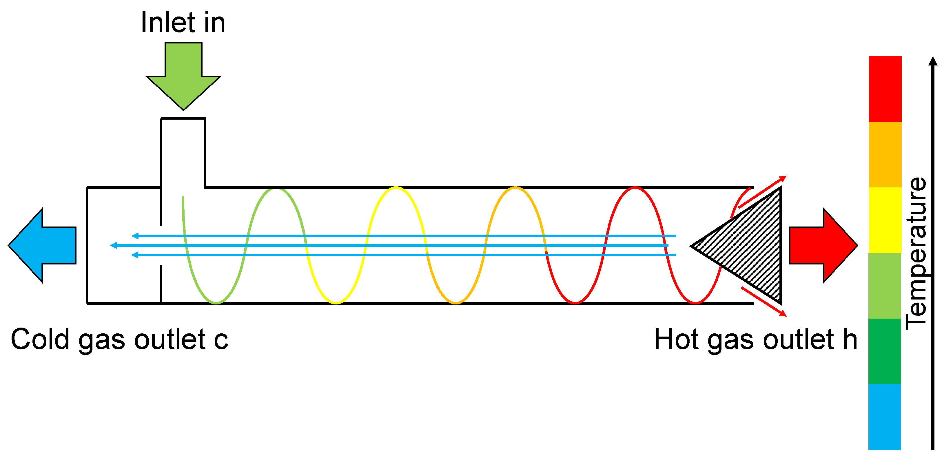
The fundamental principle of the RHVT involves the tangential entry and expansion of a high-pressure fluid through one or several nozzles, causing the flow to rotate within the tube. As a result, a stream of gas, referred to as the hot gas stream, emerges near the opposite end of the entry point with a higher temperature than the inlet stream. Simultaneously, a second stream, known as the cold gas stream, emerges as a core flow near the inlet with a reduced temperature compared to the inlet. The schematic layout and temperature distribution are depicted in Figure 1.
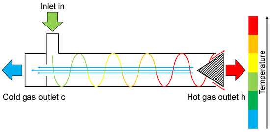
Figure 1.
Schematic layout and temperature distribution of the vortex tube.
The mass flow rates of the two streams can be adjusted using a valve (indicated by the hatched area in Figure 1). In the literature, usually only the cold gas mass flow fraction is referenced, which describes the ratio of the cold gas mass flow to the inlet mass flow . Thus, the hot gas mass flow fraction is given by . It is noteworthy that the maximum temperature difference of each outlet stream compared to the inlet stream occurs when its respective mass flow rate is low, as can be seen in Figure 2.

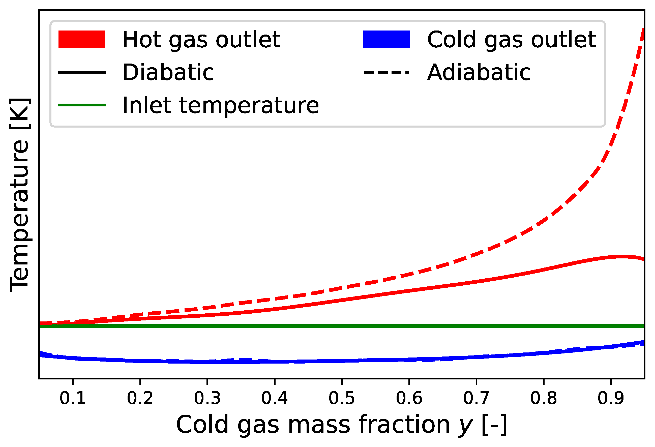
Figure 2.
Typical temperature distributions for an uninsulated and insulated vortex tube at a constant pressure ratio (cf. Keller et al. [3]).
To date, the exact mechanism(s) causing the temperature separation effect in the vortex tube has not been conclusively determined. Devade [4] provides a good overview of the multitude of theories. The authors largely agree that the actual effect may end up being a combination of several explanation approaches. However, according to Devade [4], in addition to mass flow fractions, the following influencing factors have been identified:
- The working fluid;
- Geometric factors of the vortex tube;
- The number and type of nozzles used;
- The inlet pressure or pressure ratio (following Keller et al. [3]);
- The inlet temperature;
- Phase change during expansion (cf. [5]).
To unravel the mechanism of the vortex tube and its influencing parameters, numerous experimental studies have been carried out. Regarding the length and diameter of the vortex tube ( and ) as well as the diameter of the cold outlet orifice diameter (), the experiments identified optimal geometrical ratios (i.e., and ) (cf. [6]). Moreover, the experimental evaluations have led to the insight that increasing inlet pressures and an increasing number of nozzles can enhance temperature separation at both outlet streams (cf. [3,7,8]). However, the increase in temperature separation is limited to a certain pressure ratio and number of nozzles. A comprehensive overview of the experimental results can be found in [9,10,11].
Furthermore, the particular influence of the thermal insulation of the vortex tube on the temperature separation effect has been discussed by several authors [3,7,12,13]. If the cold gas mass flow fraction y is close to its boundaries 0 or 1, a significant temperature decrease for the cold gas temperature and an increase for the hot gas temperature can be observed, respectively. This leads to non-negligible heat exchange with the environment. Stephan et al. [7], Thakare and Parekh [12] and Promvonge and Eiamsa-ard [13] showed that for insulated vortex tubes, the temperature difference to the inlet can be increased for both the hot and cold outlet sides. Keller et al. [3] also point out that if the insulation is satisfying, the otherwise typical temperature drop to y-values close to one can be suppressed, and the temperature difference increases progressively towards the limit of (cf. Figure 2).
In addition to experimental work, model-based analyses constitute the second major group of scientific work on the Ranque–Hilsch vortex tube. These can be broadly divided into numerical investigations using CFD software tools and analytical models involving fluid mechanical and/or thermodynamic considerations. The main objective of CFD studies is to extend the knowledge gained from the experimental work. Different working fluids and a wider range of geometry variations can be tested while minimizing the resources required (cf. [14,15,16,17]). Furthermore, the CFD results can provide a deeper understanding of the temperature separation effect inside the vortex tube. A comprehensive overview of CFD-based investigations and their results can be found in [9,18].
On the other hand, analytical modeling approaches were carried out to estimate the vortex tube performance in a particular application. Therefore, early approaches to analytical modeling of the temperature separation effect were limited to predicting maximum achievable temperature differences or predicting the operating range. Nowadays, analytical models are based on two different approaches:
- Fluid mechanical approaches;
- Thermodynamic black-box approaches.
As the name indicates, fluid mechanical modeling approaches attempt to describe the temperature separation behavior with basic fluid mechanical equations (i.e., conservation of mass, impulse, and energy) describing the fluid behavior inside the vortex tube. Thereby, fluid mechanical approaches depend on the geometrical information of the vortex tube. Furthermore, since the mechanism of the temperature separation effect is not yet clear, fluid mechanical models often rely on empirical constants that are fitted to measurement data (cf. [19]) or a lot of assumptions (cf. [20]).
Regarding thermodynamic black-box approaches, the energy and entropy balance for steady-state flow processes can be formulated for the vortex tube (cf. Equations (1) and (2)), and the two unknown outlet temperatures (i.e., and ) can be determined. Thereby, the internal mechanism responsible for temperature separation is treated as a black-box, which is represented by the irreversible entropy generation . To define the behavior of the irreversible entropy generation for different geometric and operating conditions, different simple parameter sets are defined [3,21,22,23,24].
Today, vortex tubes are mainly used for cooling applications or for material separation [25,26]. Nevertheless, there are ideas for using the hot outlet of the vortex tube in processes like Rankine, Brayton, or heat pump cycles [3,24,27]. Performance estimation models are needed to assess its potential within thermodynamic cycles. However, the given modeling approaches for RHVTs show weaknesses, which will be discussed in detail in the following section of the present study. To overcome these weaknesses, a simple yet comprehensive modeling approach was developed. It covers the influence of the main process parameters (e.g., , , , and y) on the temperature separation effect while allowing fast computation. In that way, the present study presents a new analytical approach to assess the vortex tube performance based on the theoretic principles behind the vortex tube effect.
2. Methodology
The following subsections shall provide fundamental insights into the derivation and evaluation of the developed modelling approach to determine the vortex tube performance in different applications. Therefore, to better understand the necessity of a new model, the different modeling approaches are reviewed, and their respective weaknesses are discussed.
2.1. Review of the Available Vortex Tube Modeling Approaches
As mentioned before, the first performance estimation approaches of the vortex tube are restricted to describing the maximum performance of the vortex tube. For example, Fulton [28] derived an expression for the maximum temperature difference on the cold gas side depending on the turbulent Prandtl number. Ahlborn et al. [29] formulated comparable limits for the achievable hot and cold gas temperatures relative to the inlet temperature, depending on the pressure difference. The approach considers a second vortex between the hot and cold flows. In a later work, they formulated an expression for the occurring temperature differences via the cold gas mass flow fraction y and the de-dimensionalized pressure difference X as well as the isentropic exponent . In contrast, Stephan et al. [7] formulated an empirical equation for the temperature difference on the cold gas side for geometrically similar vortex tubes. The equation depends on the cold gas mass flow fraction y, while the influence of the pressure difference is not considered. Piralishvili and Fuzeeva [30] provided an empirical formula but included other quantities such as the Reynolds and Prandtl numbers.
The most discussed fluid mechanical modeling approaches of the vortex tube were proposed by Shannak [19] and Mansour et al. [20]. Shannak [19] related temperature separation to friction losses in the vortex tube. For this purpose, he established the Bernoulli equation for both partial flows. Together with energy and mass conservation, this resulted in Equations (3) and (4) for hot and cold gas temperature.
The parameters and describe empirical friction factors that depend on the pressures and , the inlet temperature , and the cold gas mass fraction y.
In contrast to Shannak [19], Mansour et al. [20] did not consider empirically determined equations. Instead, they modeled the working fluid with an equation of state for real gases. Assuming that the velocities of the vortex are much higher in the circumferential direction than in the axial or radial direction and that the largest velocity changes occur along the radius, a computational path is defined, which can be used to determine hot and cold gas temperatures.
Thermodynamic black-box modeling approaches have been presented by Keller et al. [3], Mischner and Bespalov [21], Liu et al. [22], Zhao and Ning [23], and Cetin and Zhu [24]. All authors have developed one parameter that condenses all geometric and operational conditions but differs in its implementation.
To better understand the approaches of Keller et al. [3] and Mischner and Bespalov [21], a closer look at experimental results considering the irreversible entropy production may be helpful: O’Connell [31] examined the Equations (1) and (2) for different working fluids in the vortex tube and concluded that is lower than the entropy generation of an adiabatic throttling valve with the same inlet and outlet pressure. The exact difference between both irreversible entropy generations depends on the cold mass fraction y and the pressure difference between the inlet and the outlet. Saidi and Yazdi [32] stated a similar finding for exergy losses, which are closely related to entropy generation. Thereby, the entropy generation of a throttling valve is determined for the same inlet and outlet pressures using an entropy balance (cf. Equation (5)). The pressure difference between hot and cold gas outlets is neglected in the investigations presented.
Following those findings, Mischner and Bespalov [21] formulated a relation for the reduction of entropy generation compared to the adiabatic throttling valve via an efficiency parameter and a flow parameter, the Rossby number . Thus, for ideal gases, they determined a “separation entropy” depending on a theoretically maximum separation entropy by which the throttling valve associated entropy generation is reduced by the vortex tube (cf. Equations (6) and (7)). depends on the cold mass fraction y, as can be seen in Equation (8), and is derived from an analogy between temperature separation and stream separation of a single-component flow.
Keller et al. [3] chose a similar but strongly simplified approach to describe . It is assumed that the entropy generation of an adiabatic throttling valve is reduced linearly dependent on the cold mass fraction y (cf. Equation (9)). In Equation (9), R is the mass-specific gas constant, and H is the so-called vortex tube coefficient, which depends on the specific vortex tube used and which has to be determined experimentally.
Keller et al. [3] further considered the change in velocities in the energy conservation formula (cf. Equation (10)), which was neglected by Mischner and Bespalov [21]. With known geometrical parameters, the velocities can be determined by the continuity equation (cf. Equation (11)).
Liu et al. [22], Zhao and Ning [23], and Cetin and Zhu [24] used isentropic nozzle efficiency in their calculations to compute a virtual state point (index n), from which the vortex tube outlet flows split isobarically (cf. Equation (12)). Thereby, the enthalpy at the virtual state n was inserted to determine the inlet enthalpy in Equation (1). As a second equation, the irreversible entropy generation must be greater than or equal to zero (cf. Equation (13)).
The objective of the present study is to develop a vortex tube model capable of simulating the temperature separation effect for an arbitrary fluid. Therefore, next to applications using gaseous fluid, the model should be capable of depicting its behavior for a supercritical fluid as for the Joule cycle proposed by Cetin and Zhu [24]. Since the supercritical operating range has not been studied for vortex tubes yet, the modeling approaches presented previously cannot be directly validated using experimental data. However, the qualitative behavior of the vortex tube effect, depending on the operating parameters mentioned, can be investigated for different phases.
An important relationship to consider is the dependence of temperature separation on the cold gas mass flow fraction y and the pressure difference between inlet and outlet streams. At the same time, ensuring thermodynamically correct results from the modeling approach is crucial: the entropy generation of the vortex tube model should align with the range defined by existing measurements in the subcritical region. Promising modeling approaches include the two fluid dynamics models by Shannak [19] and Mansour et al. [20], as well as the three thermodynamic black-box models developed by Keller et al. [3], Mischner and Bespalov [21], and Liu et al. [22]. Table 1 provides an overview of the individual advantages and disadvantages of these models.

Table 1.
Overview of advantages and disadvantages of investigated vortex tube models.
The advantage of the modeling approach presented by Shannak [19] is that the temperature of the hot and cold sides can be directly evaluated through formulas. There is no need for an iterative process or any pre-calculations. However, a significant drawback of this modeling approach is that Shannak [19] does not consider essential factors influencing the vortex tube effect. Thus, different vortex tube geometries can lead to entirely different results, as well as the use of different working fluids (see [5,33,34,35]) or thermal insulation (see [3,7]).
The model proposed by Mansour et al. [20] offers the advantage of real gas behavior consideration and has been validated with existing experimental data. However, the underlying experimental data from Zhu [36] were not taken systematically across different values of y or specific pressure ratios. Therefore, the quality of the experimental data and the accuracy of the calculated temperatures cannot be assessed reliably. Another issue with the model proposed by Mansour et al. [20] is the assumption that the static temperature at the cold gas outlet is equal to the static temperature at the inlet. According to this assumption, the differences in total temperature at the inlet and cold gas outlet would only consider variations in fluid velocities. However, there is no evidence in the existing literature supporting this conclusion.
Furthermore, a general challenge in flow-based models is the consideration of geometric parameters. Based on the general understanding of vortex tubes, it is difficult to estimate whether the optimal geometric ratios derived for air, regarding the maximization of temperature separation, would also apply universally to subcritical or supercritical fluids. Additionally, it is unknown whether the existing geometries can be linearly scaled up or down based on the available mass or volume flows.
Therefore, models that consider the geometric design through a simple parameterization are desirable. This is the case for models that solely rely on thermodynamic conservation equations. For example, Keller et al. [3] proposed a pipe coefficient H, which accounts for the influence of geometric parameters, while Mischner and Bespalov [21] introduced the Rossby number . Another advantage of these modeling approaches is the relatively fast solution process. Mischner and Bespalov [21] allow for direct evaluation of the desired temperatures, while Keller et al. [3] only require solving a simple set of equations with low computational effort.
However, both models encounter challenges in calculating the irreversible entropy generation of the vortex tube, denoted as . In the case of Mischner and Bespalov [21], this is achieved by calculating a separation entropy generation , which partially compensates for the throttling entropy generation. The required variable, (cf. Equation (7)), is derived through the analogy between the separation of a single-component stream and thermal separation. The equation used is the mixing equation for ideal gas mixtures (Equation (14)). Mischner and Bespalov [21] acknowledge that this formula is not applicable to single-component flows. This phenomenon is known as the “Gibbs paradox” and is attributed to the discontinuity between “very similar” and identical gases (see [21], S. 35). Nevertheless, the same formula (i.e., the mixing equation for ideal gas mixtures) is subsequently used for the analogy of identical gases, resulting in an expression for the theoretical separation entropy generation, as shown in Equation (8).
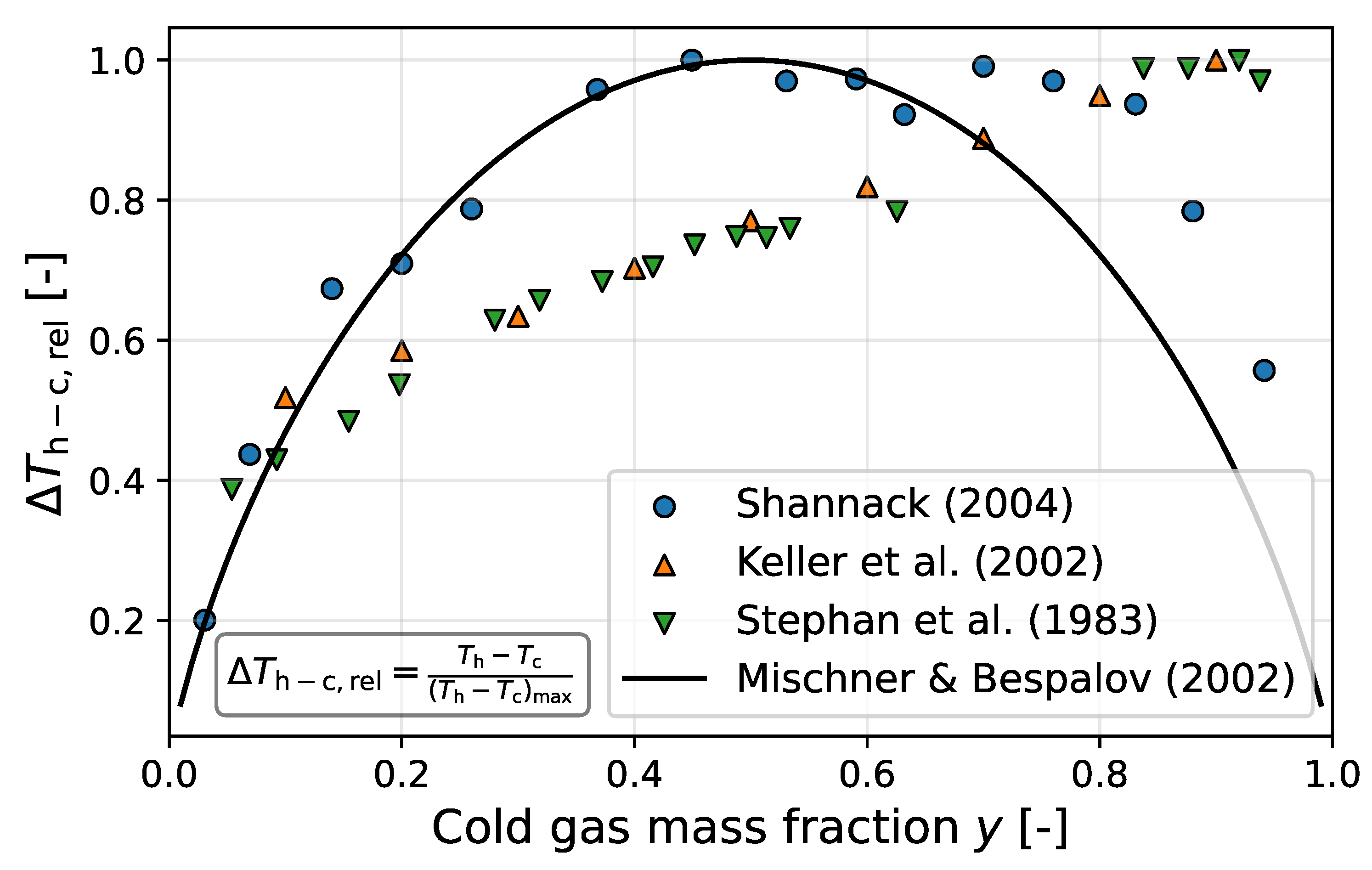
It is not clear if this approach is permissible in this case. Instead, parallels between the behavior of the theoretical separation entropy generation and the relative temperature difference between both outlets (definition in Figure 3) are referenced. Although these parallels are observed in the measurements by Shannak [19], other data sets, such as those from Keller et al. [3] or Stephan et al. [7], exhibit a less symmetric behavior with peaks shifted to higher values of y (see Figure 3). The black curve in Figure 3 does not represent actual data; instead, it represents the theoretical expectation of Mischner and Bespalov [21] based on the behavior of . Furthermore, the calculation of the efficiency employs the formula for . is based on a linear relationship between the current Rossby number and a maximum efficiency, which, based on several intermediate steps, ultimately relies on the assumed maximum of at (see Figure 3).
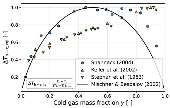
Figure 3.
Dimensionless temperature differences between hot gas and cold gas outlet of the vortex tube for the measured data of Keller et al. [3], Stephan et al. [7], and Shannak [19] compared with the theoretical course according to Mischner and Bespalov [21] (in each case for ).
The vortex tube coefficient H proposed by Keller et al. [3] does not have a theoretical basis and needs to be determined experimentally. However, the authors observed that for increasing pressure differences at a constant vortex tube coefficient H, the temperature separation decreases. This is due to the fact that as the pressure difference increases, the irreversible entropy generation of the throttling valve increases while the compensating term remains constant. As a result, the compensated portion decreases relative to the total entropy generation. However, this effect does not align with the observations made in experimental investigations. Consequently, the vortex tube coefficient should be represented as a function of the pressure and . The influence of both parameters can be derived using experimental data. However, it is unclear how the pressures interact with the vortex tube coefficient H. Furthermore, due to the lack of usable data for fluids other than air in vortex tubes, it is unknown whether the analysis of H for air can be directly applied to other fluids. It should be emphasized that there is no trivial upper limit for the vortex tube coefficient. Therefore, estimating potential deviations of the real coefficient is challenging.
The nozzle efficiency approach proposed by Liu et al. [22], Zhao and Ning [23], and Cetin and Zhu [24] offers the advantage of simple and rapid calculations, similar to the previously discussed thermodynamic modeling approaches. However, some calculation steps remain unclear, as will be discussed in the following. Firstly, the formulas used by Liu et al. [22] and Zhao and Ning [23] do not indicate how the enthalpy at the virtual state n (calculated using the nozzle efficiency ) is used. Instead of replacing the inlet enthalpy in the energy balance in Equation (1) with , the energy balance is applied to the inlet and the two outlets of the vortex tube. Only the work of Cetin and Zhu [24] shows that the energy balance replaces the inlet condition with the nozzle exit condition. Secondly, the proposed method would result in a non-isenthalpic process. For nozzle efficiencies greater than zero, the enthalpy at the virtual state n is smaller than the vortex tube inlet enthalpy. However, the origin of the enthalpy difference between the vortex tube inlet and the virtual state n remains unclear. A possible conversion into kinetic energy could solve the dilemma but is neither discussed nor introduced into the corresponding energy balance. Moreover, since both outlet states are unknown, a second equation would be required to obtain a unique solution. However, the proposed system of energy balance combined with the condition that the irreversible entropy production must be greater than or equal to zero leads to infinite possible solutions (e.g., the trivial solution of ). To achieve a unique result, alternative conditions or constraints would be necessary, which are also not discussed.
2.2. Derivation of New Black-Box Modeling Approach
As evident from the advantages and disadvantages of the above-discussed modeling approaches, a new simple thermodynamic black-box model needs to be developed for calculating the irreversible entropy generation of the vortex tube. For this purpose, an intermediate parameter from Mischner and Bespalov [21] can be employed, referred to as the vortex tube efficiency in this work. According to Equation (15), is determined by the ratio of irreversible entropy generation in the vortex tube to the entropy generation of a throttling valve.
As the irreversible entropy generation of the vortex tube is reduced by the temperature separation effect (compared to the one of the throttling valve), a fixed range of is given. A vortex tube efficiency of zero corresponds to an adiabatic throttling valve, while represents an isentropic vortex tube. cannot be exceeded, as it would result in negative irreversible entropy generation of the vortex tube, violating the second law of thermodynamics. Negative values of are also not possible, as the effect of temperature separation is closely linked to the reduction in entropy generation compared to a simple throttling valve. This can be explained well using the entropy balance for ideal gases in the vortex tube, as presented by Mischner and Bespalov [21], shown in Equation (16).
For ideal gases, the entropy generation can be clearly divided into a pressure-driven component and a temperature-driven component . Here, corresponds to the entropy generation of an isenthalpic throttling valve. Thus, must represent the separation entropy. Under the condition that , it follows that for all possible ratios and .
By using literature data and considering the value range, the behavior of across different pressure ranges and y-values can be investigated, ultimately leading to the derivation of a formula for . Finally, Equation (17) can be employed to determine the vortex tube entropy.
2.3. Evaluation of Measured Data
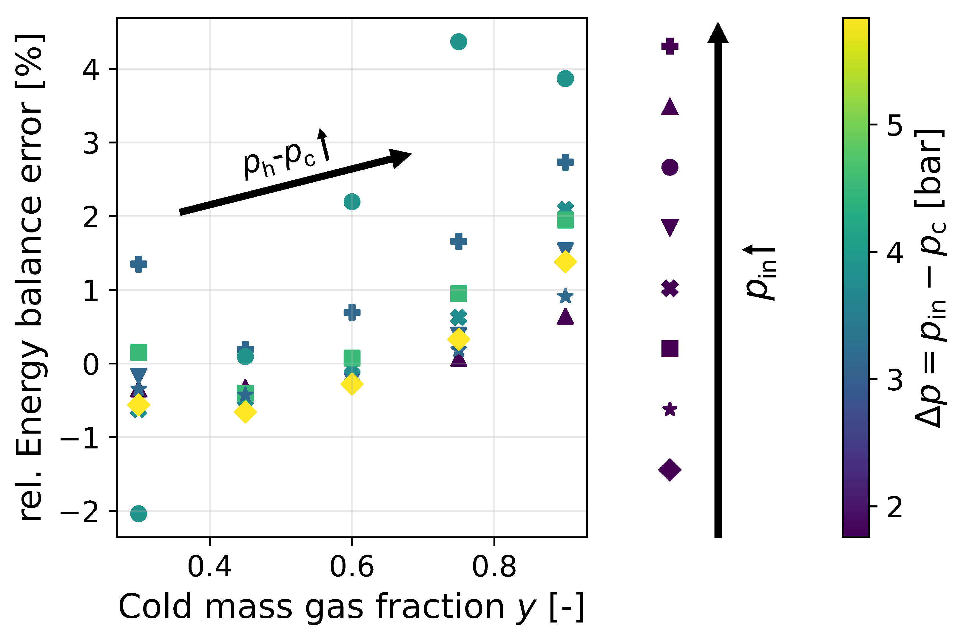
Studying the energy balance for different sets of experimental data from the literature, it can be seen that there is a disparity between the enthalpy at the inlet and the sum of the two enthalpies of the outgoing substreams (cf. Figure 4). This phenomenon may have several causes, which cannot be precisely differentiated from each other due to a lack of information in the literature. Neglecting the pressure difference () may have an influence. The data provided by Parker and Straatman [8] document both outlet pressures. While the pressure at the cold gas outlet remains constant, the pressure at the hot gas outlet is greater than for increasing y. However, the data in Figure 4 show that neglecting the pressure difference between the two outlets is not the only reason for the energy balance error.

Figure 4.
Error of mass-specific energy balance relative to inlet enthalpy for Parker and Straatman’s [8] results.
Another reason can be the change in velocity between the inlet and outlets, which is typically not measured. This would require information on the diameters or cross-sectional areas of the respective measuring planes, which are usually not given.
The third possible cause of the imbalance in the energy balance is insufficient insulation of the vortex tube. As shown by Keller et al. [3], very high temperatures can be reached on the hot side for sufficiently high y-values if the insulation is adequate. At the same time, these adiabatic vortex tube temperatures offer great potential for heat transfer to the environment if insulation is inadequate. On the other hand, the cold side offers the potential for heat transfer from the environment. These two heat transfer effects cannot be separated in their sum. Because of the inequality in the energy balance, three ways of balancing entropy are considered:
- Neglect of the inequality of the energy balance;
- Correction of the entropy balance by means of heat flow;
- Correction of one output flow enthalpy and adiabatic entropy balance.
As a reference point, the temperature data provided in literature are evaluated without any corrective measures. Accordingly, the irreversible entropy generation at the vortex tube is given by Equation (18). Via Equation (19), the separation entropy follows as the difference between entropy generation of the throttling valve (cf. (5)) and the vortex tube.
If the corrections are applied, it is assumed that the influence of altered outlet pressures and the velocities of the cold and hot sides can be neglected since the data for a more precise calculation are lacking in the literature. Accordingly, all inequalities of the energy balance are accounted for by the heat transfer with the environment. In both correction approaches, the transferred heat flux is determined from the energy balance (Equation (20)). The heat flux is assumed to be an outgoing heat flux in the balance: if it results in a negative sign, it enters the vortex tube. Since only the sum of all heat flows is considered and no differentiation can be made between the heat transfer of the cold outlet and the hot outlet, the resulting heat flow is attributed to the side corresponding to the sign of the heat flux.
For the first correction approach (corr. V1), this results in a correction of the entropy balance by the transferred heat flux, which adds or removes entropy at a certain transfer temperature (cf. Equation (21)). The transfer temperature is thereby determined as the temperature of the heat-transferring partial mass flow.
The second approach (corr. V2) corrects the enthalpy of the heat-transferring partial flow (cf. Equations (22) and (23)). The resulting adiabatic enthalpy, , can then be used to calculate an adiabatic temperature or an adiabatic entropy . The irreversible entropy generation is calculated using Equation (21), where the adiabatic entropy is used for the heat-transferring partial flow. A supporting visualization of the proposed correction variants can be found in the Supplementary Data (Figure S1).
The results of the proposed entropy analysis are discussed below using measured data from Keller et al. [3], Stephan et al. [7], Shannak [19], Parker and Straatman [8], Sarifudin et al. [37], Promvonge and Eiamsa-ard [13], and Majidi et al. [38] regarding air as a working fluid. In addition, the data of Zhu [36] for CO2, Williams [33] for methane, and O’Connell [31] for helium were considered. Fluid property values for the calculation were obtained using the Python (version 3.10.9) module Coolprop (version 6.4.3). Major assumptions can be found in Table 2. Results not reported in the paper can be found in the Supplementary Data (Figures S2–S74).
Table 2.
Assumptions of the vortex tube efficiency evaluation of the present study.
3. Results
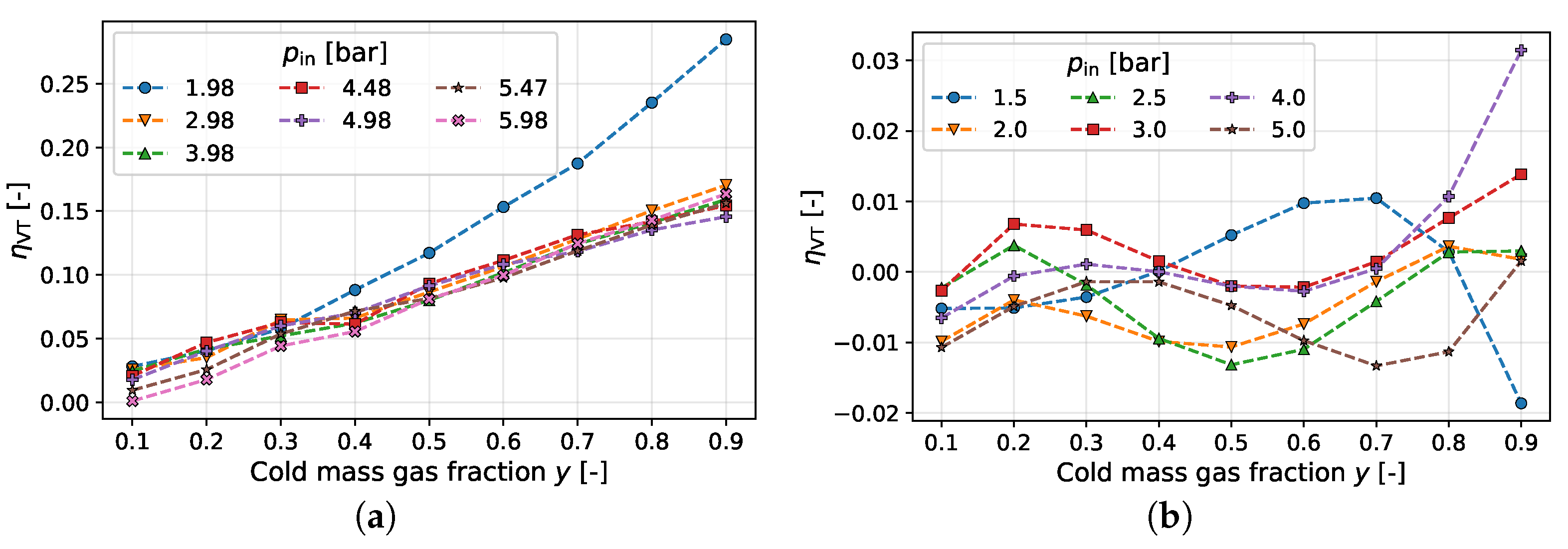
First, the effect of the corrections was evaluated and compared to the calculation without correction. Figure 5a,b exemplarily shows the resulting vortex tube efficiency of the studies conducted by Keller et al. [3] and Stephan et al. [7] for different inlet pressures and cold gas mass fractions. The corresponding corrected values can be seen in Figure 6a,c, respectively.
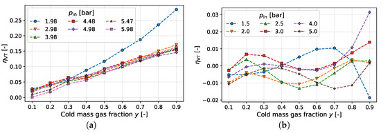
Figure 5.
Uncorrected results for versus cold gas fraction of different pressure studies. (a) Keller et al. [3]. (b) Stephan et al. [7].
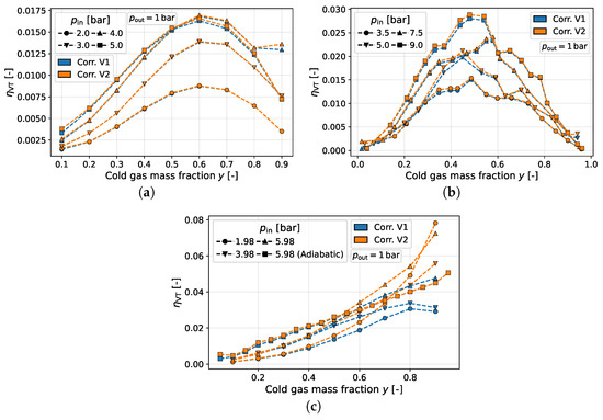
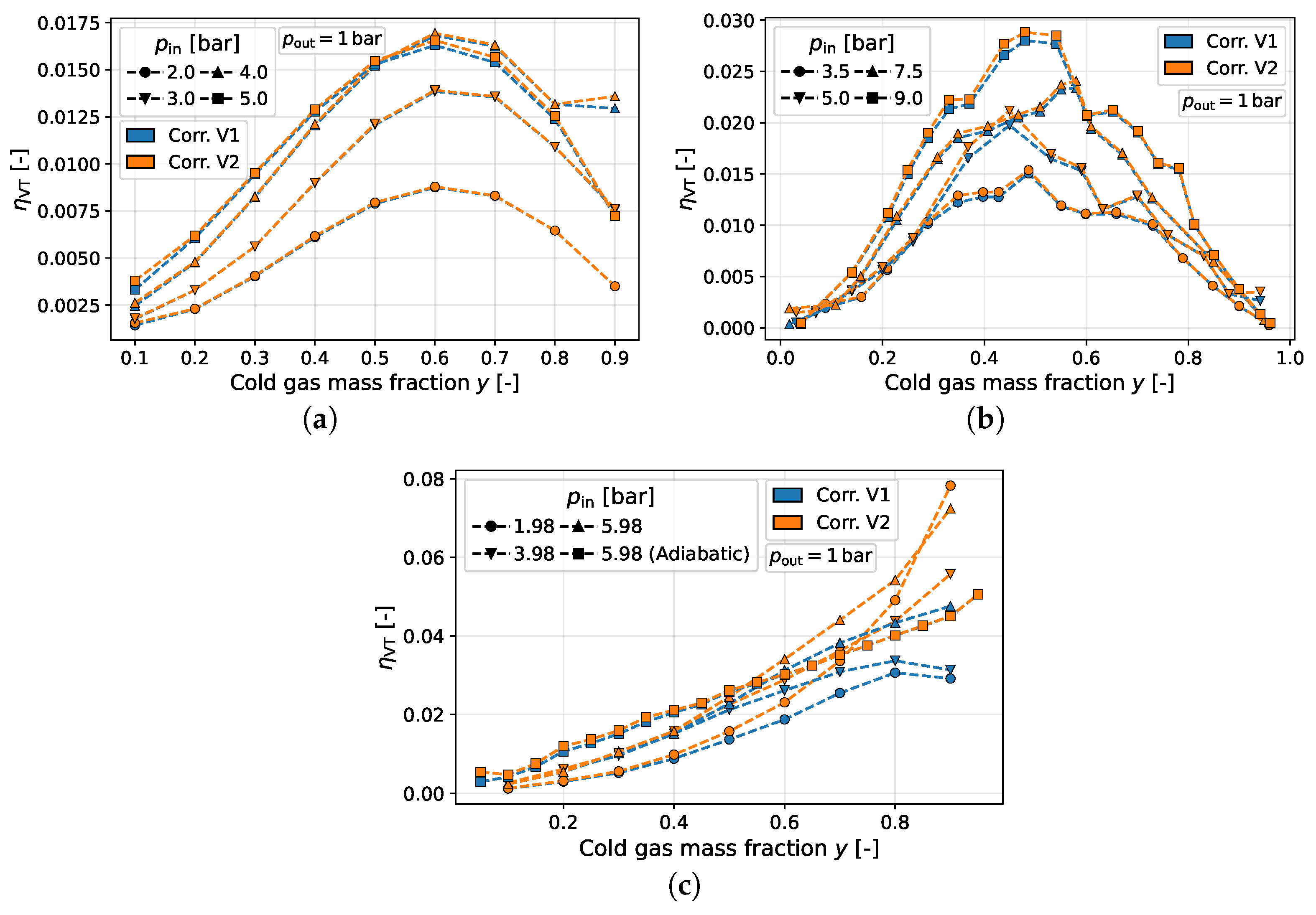
Figure 6.
Corrected results for versus cold gas fraction for different studies with air. (a) Stephan et al. [7]. (b) Shannak [19]. (c) Keller et al. [3].
In the data of Keller et al. [3], all values for are already in the positive range before correction; the data presented by Stephan et al. [7] are distributed almost symmetrically around . However, as has already been discussed, a negative sign for is not thermodynamically meaningful. In addition to the negative values, the data provided by Stephan et al. [7] illustrate that only through the correction a clear structure or trend for becomes apparent (see Figure 6a). For the results presented by Keller et al., [3] the qualitative behavior of the results versus y remains similar for all three computational methods. On the other hand, the results presented by Keller et al. [3] show a big difference in the absolute values for : the efficiency of the uncorrected version reaches up to 25%, while only a maximum of 8% is seen in the corrected versions (cf. Figure 6c). The reason for this behavior is high heat fluxes, which removes entropy from the system. In the uncorrected version, this dissipated fraction of entropy is also credited to the separation entropy, which thus increases and consequently causes to increase. The same reasoning can be applied to explain negative efficiencies. When heat is transferred from the ambient to the cold side, entropy is introduced into the system. Thus, the sum of the entropy generation is greater than that of the entropy generation, which is compensated for by the separation effect. This results, without correction, in a larger than the entropy generation of a throttling valve, and thus a negative vortex tube efficiency.
In the following, based on the previous findings, only the correction variants are examined. However, the corresponding uncorrected results can be found in the Supplementary Data.
3.1. Cold Gas Mass Fraction Influence
As stated before, the cold gas mass fraction has a crucial influence on the outlet temperatures. To investigate the corresponding influence of the cold gas mass fraction on the vortex tube efficiency, Figure 6 illustrates the results of versus y for the data provided by Stephan et al. [7], Shannak [19], and Keller et al. [3] at different inlet pressures. Overall, two trends for can be identified for both correction variants:
- A maximum turning point;
- A steady increase.
On the one hand, there are measured data for which the efficiency increases versus y up to a certain point and then decreases again. In this case, the maximum for is located between . Examples include the data of Stephan et al. [7] and Shannak [19] (cf. Figure 6a,b). Hereby, the reason behind the position of the optimum of over the cold gas mass fraction cannot be identified. However, the optimal cold mass fraction of the different data sets does not seem to have a dependency on the inlet pressure or pressure ratio. Further examples can be found in the Supplementary Data.
On the other hand, some data sets show a steadily increasing efficiency, as in Figure 6c for the data set of Keller et al. [3]. While the first correction variant shows both trends, the second correction variant shows only the steadily increasing efficiency. Special attention should be paid here to the slope of the efficiency, which must not be constant (i.e., linear increase) but may also increase steadily. Furthermore, Figure 6c shows the adiabatic results of Keller et al. [3], which also indicate a linear trend of over y. As a result, it can be observed that the vortex tube efficiency increases for increasing . Regarding , further experimental investigations are necessary to fully understand the differences between the observed trends.
3.2. Pressure Influence
Similar to the effect of cold gas mass fraction, the effect of inlet and outlet pressures can be studied. In most experimental investigations of the influence of pressure on the temperature separation effect, only the inlet pressure is varied. Thus, for these investigations, the pressure difference and the pressure ratio both represent only the change in the . For this reason, one of the two quantities can be omitted, which is why only the behavior of versus the pressure ratio is shown in these cases. The corresponding Figures S33–S47 for the pressure difference can be found in the Supplementary Data.
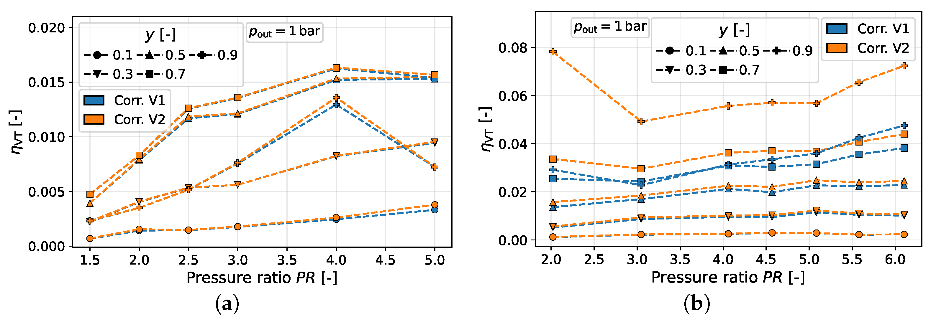
Figure 7a shows the dependence of the vortex tube efficiency versus the pressure ratio for both correction variants, considering the data of Stephan et al. [7] and Keller et al. [3].
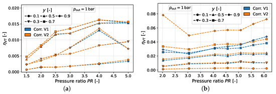
Figure 7.
Corrected results for versus pressure ratio for different pressure studies. (a) Stephan et al. [7]. (b) Keller et al. [3].
Overall, inlet pressure variations do not show a clear behavior for . For the study of Stephan et al. [7], very similar curves are shown for both correction variants: a rather linearly increasing trend of the vortex tube efficiency can be observed for the data points associated with lower y-values. For higher y, the progression of with a rising pressure ratio seems to be limited. In contrast, the results of Keller et al. [3] demonstrate a greater quantitative variation in behavior between the correction variants, particularly for smaller pressure ratios and high y-values (cf. Figure 7b). In the high y-range, the efficiency for correction variant two decreases by several percentage points with an increase in the pressure ratio before it increases again. This is also the case for the first correction variant, but the drop in efficiency is much less pronounced, and the increase in efficiency with is dominant. For low y-values, it should also be noted that the efficiency is almost constant.
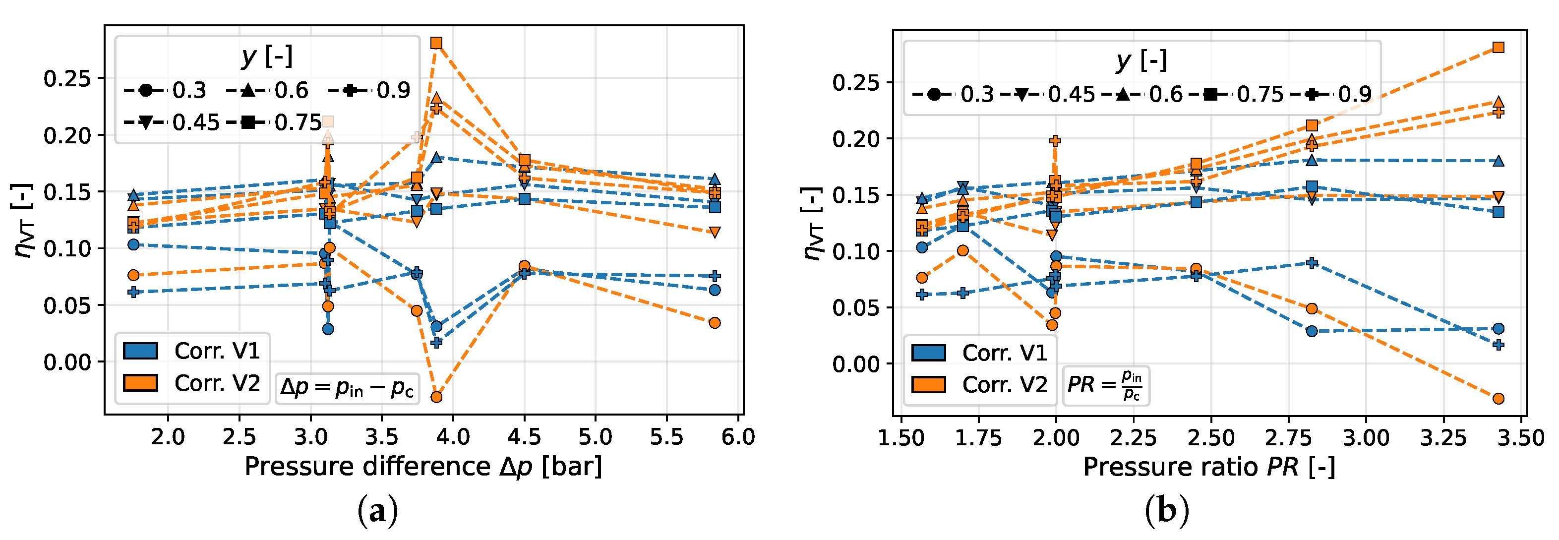
Furthermore, the data provided by Parker and Straatman [8] are examined, who varied both inlet and outlet pressures. Figure 8a shows the vortex tube efficiency at different pressure differences, and Figure 8b represents the efficiency at different pressure ratios.
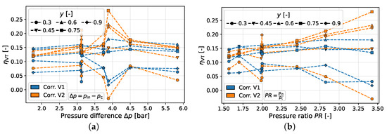
Figure 8.
Corrected results for versus pressure difference and pressure ratio for the study of Parker and Straatman [8]. (a) Dependence on . (b) Dependence on .
For the pressure differences, no clear trend can be seen for both correction variants. The vortex tube efficiencies at are associated with the highest pressure ratios, so values are peaking. Otherwise, the efficiencies appear to be constant (corr. V1) or slightly increasing (corr. V2). Only for is a slight decrease observed for both correction variants.
Looking at the pressure ratio, clearer trends can be seen, although these trends differ depending on their associated y-value. Thus, for correction variant one, a downward trend with an increasing pressure ratio can be seen for and for , whereas the efficiency slightly increases or remains constant for the remaining y-values.
For correction variant two, the decreasing efficiency is only observed for , while for y-values higher than , the efficiency increases with the pressure difference instead. Furthermore, the increase in efficiency is quantitatively more pronounced (for , it rises above 15%).
3.3. Further Influences of the Vortex Tube Efficiency
Finally, individual aspects regarding the vortex tube efficiency shall be investigated further. For example, the behavior of the vortex tube with and without thermal insulation was investigated by Keller et al. [3], Stephan et al. [7], and Promvonge and Eiamsa-ard [13]. For the results of Keller et al. [3], a distinct linear behavior of versus the cold gas mass fraction can be observed (cf. Figure 6c). However, for the results provided by Stephan et al. [7] and Promvonge and Eiamsa-ard, [13] no qualitatively or quantitatively significant difference or distinct trend was witnessed between insulated and non-insulated measurements for the vortex efficiency after the application of the correction variants. Therefore, to avoid redundancy, the results of Stephan et al. [7] and Promvonge and Eiamsa-ard [13] can be found in the Supplementary Data (Figures S48–S56). The vortex tube effect has also been investigated for media other than air. Unfortunately, complete data sets for evaluation are lacking. Usually, several media are directly compared with each other, and only maximum values for temperature separation are given. Nevertheless, the vortex tube efficiency was analyzed for available data comprising helium, methane, and CO2. The corresponding Figures S57–S74 for the vortex tube efficiency can be found in the Supplementary Data. Overall, the same observations as for air can be carried out for all evaluated working fluids: the vortex tube efficiency of methane over the cold gas mass fraction evaluated for the measurements reported by Williams [33] appears to have a maximum for lower inlet pressures, while for higher inlet pressures a linear trend over y is present. For helium, O’Connell [31] provides an extensive data set. Here, the differences in vortex tube entropy generation compared to the throttling valve (i.e., ) are provided directly. Thus, no separate heat flux correction can be performed. The method described by O’Connell [31] seems to correspond to correction variant one. Evaluating the vortex tube efficiency versus y, O’Connell’s [31] data show a maximum in vortex tube efficiency at . For the pressure influence, only the was varied. An increase in vortex tube efficiency for small pressure ratios can be seen for all y-values considered, whereas larger pressure ratios do not cause any further increase in the vortex tube efficiency; in fact, it can also drop. The vortex tube efficiencies for the data set provided by Zhu [36] lack a systematic measurement scheme for either constant pressures or constant y. Therefore, it is not possible to identify a trend for these two influencing factors and match it with the findings for air. Despite this, a lot of the calculated efficiencies can be classified at 20%. This shows that efficiencies in the order of Parker and Straatman’s data [8] for air are not unrealistic for other media (here ) either.
4. Discussion
Considering the presented evaluations of the vortex tube efficiency, a function of the vortex tube efficiency shall be formulated, which depicts the crucial influencing parameters of the vortex tube performance. A simple approach is to express the function as a product of subfunctions, each of which depends exclusively on a single influencing parameter (cf. Equation (24)). It should be noted that the assumption of non-interdependence has not yet been sufficiently validated. In particular, depending on the cold gas mass fraction y, the evaluation of the pressure influence has shown different trends. Therefore, further systematic measurements are required to explore the influence of the inlet and outlet pressure on the vortex tube efficiency.
Regarding the influence of the cold gas mass fraction, a trend curve with a maximum and a steadily increasing trend could be observed. Thus, a linear function serves as a compromise between the contrary trends. Furthermore, the measurement of a thermally strongly insulated vortex tube by Keller et al. [3] shows a clearly linear trend (cf. Figure 6c). Moreover, to define more complex functions (e.g., a quadratic function), further assumptions or further knowledge (e.g., the location of a maximum) would be necessary. As a result, the subfunction was expressed in Equation (25). Thereby, the subfunction is already scaled inside the limits of the vortex tube efficiency (i.e., ) for .
Since no clear trend can be worked out regarding the influence of pressure, efficiency was assumed to be constant for different pressures. At first glance, it seems more intuitive that with increasing pressure differences or pressure ratios, the efficiency increases. However, since the evaluations also show decreasing and constant trends (cf. Figure 7 and Figure 8b), the assumption of a constant vortex tube efficiency over different operating pressures serves as a conservative estimate. The resulting subfunction is shown in Equation (26).
In addition, depends on the geometry and the working fluid. Hereby, important geometries reported in literature are the length and diameter of the vortex tube ( and ) and the diameter of the cold outlet orifice diameter () as well as their ratios (i.e., and ). Therefore, the influence of the geometry and the working fluid is condensed in the form of a reference vortex tube efficiency in Equation (27). According to the observed maximum values of the individual measurement series provided in the literature, the value of should lie between 0% and 25%. Further experimental investigations should also focus on the influence of the different geometric parameters and working fluids regarding this reference vortex tube efficiency.
Overall, the vortex tube efficiency follows Equation (28).
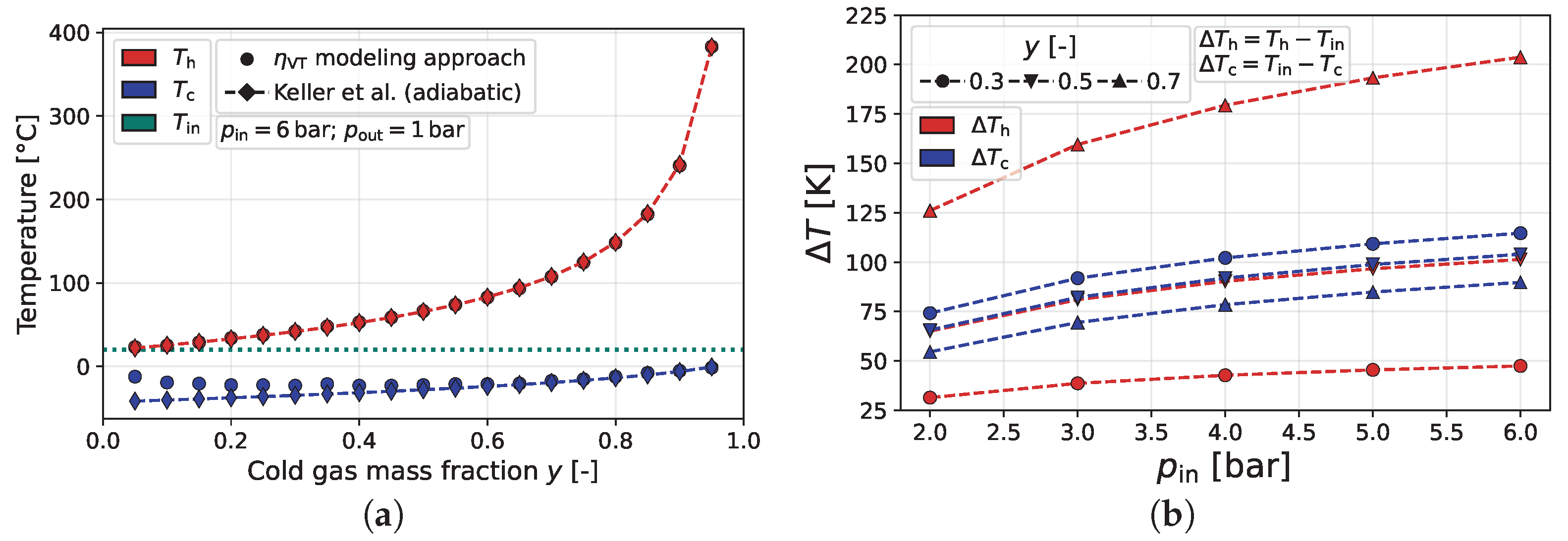
Figure 9a compares the resulting vortex tube efficiency model to the adiabatic measurements of Keller et al. [3], depicting a high quantitative precision of the proposed black-box modeling approach. In addition, Figure 9b shows the temperature separation for air at increasing inlet pressures (and constant outlet pressure). As can be seen, this model satisfies the effect of increased temperature separation for higher pressure ratios, respectively, regarding different working fluids.
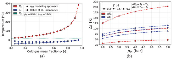
Figure 9.
Temperature separation results of the proposed black-box modeling approach for the final vortex tube efficiency model using air as a working fluid. (a) Comparison of the adiabatic measurements of Keller et al. [3]. (b) Comparison of different inlet pressures at a constant bar.
5. Conclusions
The present study aimed to investigate a simplified vortex tube modeling approach for thermodynamic performance simulations. In the first step, weaknesses of existing vortex tube modeling approaches were discussed. Based on the discussed approaches and the corresponding weaknesses, a vortex tube model was developed. The developed model is a thermodynamic black-box model using energy and entropy balances. It includes the influence of process variables (e.g., , , , and y) on the temperature separation effect by means of a defined vortex tube efficiency . The vortex tube efficiency is a new parameter introduced in this work, which describes the ratio of the reduction of the entropy generation due to the temperature separation effect and the entropy generation of an adiabatic throttling valve at the same operating pressures. To develop an expression of the influence of the different parameters on the vortex tube efficiency, experimental data provided in the literature were evaluated. The result has been the development of a vortex tube efficiency function.
The key outcomes of the present study are as follows:
- For the derivation of using experimental data, it is necessary to consider heat transfer to and from the ambient.
- The literature data do not provide a clear and comprehensive trend for the developed expression of , especially for the influence of the pressure ratio or the geometric influence.
- A simple conservative yet physical-based formulation of is capable of depicting the vortex tube behavior for air in alignment with measurement data.
The present work is limited to available data in the literature. Therefore, future work should focus on the systematic experimental investigation of the influence of the process parameters and geometries as well as the working fluid on the vortex tube efficiency. On the one hand, this means examining the dependence of the vortex tube efficiency on the pressure gradient used and to illuminate possible interdependencies between and y. In addition, the calculation approach for should also be investigated considering different aggregate states. However, the proposed expression for the vortex tube efficiency can now be used for thermodynamic performance estimations to explore the potential of the vortex tube in different applications like Rankine and Joule cycles.
Supplementary Materials
The following supporting information can be downloaded at https://www.mdpi.com/article/10.3390/en17164180/s1, Figure S1: Visualized correction scheme of the measured values; Figure S2: Relative error of the mass-specific energy balance of the data for air provided by Keller et al. [3]; Figure S3: Relative error of the mass-specific energy balance of the adiabatic data for air provided by Keller et al. [3]; Figure S4: Relative error of the mass-specific energy balance of the data for air provided by Stephan et al. [7]; Figure S5: Relative error of the mass-specific energy balance of the comparison between adiabatic and diabatic conditions for air provided by Stephan et al. [7]; Figure S6: Relative error of the mass-specific energy balance of the data provided by Shannak [19]; Figure S7: Relative error of the mass-specific energy balance of the data for air provided by Sarifudin et al. [37]; Figure S8: Relative error of the mass-specific energy balance of the comparison between adiabatic and diabatic conditions for air provided by Promvonge and Eiamsa-ard [13]; Figure S9: Relative error of the mass-specific energy balance of the data for CO2 provided by Zhu [36]; Figure S10: Relative error of the mass-specific energy balance of the data for methane provided by Williams [33]; Figure S11: -y diagram of the data for air at different inlet pressures provided by Keller et al. [3] (corr. V1); Figure S12: -y diagram of the data for air at different inlet pressures provided by Keller et al. [3] (corr. V2); Figure S13: -y diagram of the data for air at different inlet pressures provided by Stephan et al. [7] (corr. V1); Figure S14: -y diagram of the data for air at different inlet pressures provided by Stephan et al. [7] (corr. V2); Figure S15: -y diagram of the data for air at different inlet pressures provided by Shannak [19] (without corr.); Figure S16: -y diagram of the data for air at different inlet pressures provided by Shannak [19] (corr. V1); Figure S17: -y diagram of the data for air at different inlet pressures provided by Shannak [19] (corr. V2); Figure S18: -y diagram of the data for air at different inlet pressures provided by Parker and Straatman [8] (without corr.); Figure S19: -y diagram of the data for air at different inlet pressures provided by Parker and Straatman [8] (corr. V1); Figure S20: -y diagram of the data for air at different inlet pressures provided by Parker and Straatman [8] (corr. V2); Figure S21: -y diagram of the data for air at different inlet pressures provided by Sarifudin et al. [37] (without corr.); Figure S22: -y diagram of the data for air at different inlet pressures provided by Sarifudin et al. [37] (corr. V1); Figure S23: -y diagram of the data for air at different inlet pressures provided by Sarifudin et al. [37] (corr. V2); Figure S24: - diagram of the data for air at different cold gas mass fractions provided by Keller et al. [3] (without corr.); Figure S25: - diagram of the data for air at different cold gas mass fractions provided by Keller et al. [3] (corr. V1); Figure S26: - diagram of the data for air at different cold gas mass fractions provided by Keller et al. (corr. V2); Figure S27: - diagram of the data for air at different cold gas mass fractions provided by Stephan et al. [7] (without corr.); Figure S28: - diagram of the data for air at different cold gas mass fractions provided by Stephan et al. [7] (corr. V1); Figure S29: - diagram of the data for air at different cold gas mass fractions provided by Stephan et al. [7] (corr. V2); Figure S30: - diagram of the data for air at different cold gas mass fractions provided by Parker and Straatman [8] (without corr.); Figure S31: - diagram of the data for air at different cold gas mass fractions provided by Parker and Straatman [8] (corr. V1); Figure S32: - diagram of the data for air at different cold gas mass fractions provided by Parker and Straatman [8] (corr. V2); Figure S33: - diagram of the data for air at different cold gas mass fractions provided by Sarifudin et al. [37] (without corr.); Figure S34: - diagram of the data for air at different cold gas mass fractions provided by Sarifudin et al. [37] (corr. V1); Figure S35: - diagram of the data for air at different cold gas mass fractions provided by Sarifudin et al. [37] (corr. V2); Figure S36: - diagram of the data for air at different cold gas mass fractions provided by Keller et al. [3] (without corr.); Figure S37: - diagram of the data for air at different cold gas mass fractions provided by Keller et al. [3] (corr. V1); Figure S38: - diagram of the data for air at different cold gas mass fractions provided by Keller et al. [3] (corr. V2); Figure S39: - diagram of the data for air at different cold gas mass fractions provided by Stephan et al. [7] (without corr.); Figure S40: - diagram of the data for air at different cold gas mass fractions provided by Stephan et al. [7] (corr. V1); Figure S41: - diagram of the data for air at different cold gas mass fractions provided by Stephan et al. [7] (corr. V2); Figure S42: - diagram of the data for air at different cold gas mass fractions provided by Parker and Straatman [8] (without corr.); Figure S43: - diagram of the data for air at different cold gas mass fractions provided by Parker and Straatman [8] (corr. V1); Figure S44: - diagram of the data for air at different cold gas mass fractions provided by Parker and Straatman [8] (corr. V2); Figure S45: - diagram of the data for air at different cold gas mass fractions provided by Sarifudin et al. [37] (without corr.); Figure S46: - diagram of the data for air at different cold gas mass fractions provided by Sarifudin et al. [37] (corr. V1); Figure S47: - diagram of the data for air at different cold gas mass fractions provided by Sarifudin et al. [37] (corr. V2); Figure S48: -y diagram of the data for air at adiabatic conditions provided by Keller et al. [3] (without corr.); Figure S49: -y diagram of the data for air at adiabatic conditions provided by Keller et al. [3] (corr. V1); Figure S50: -y diagram of the data for air at adiabatic conditions provided by Keller et al. [3] (corr. V2); Figure S51: -y diagram of the data for air at adiabatic and diabatic conditions provided by Stephan et al. [7] (without corr.); Figure S52: -y diagram of the data for air at adiabatic and diabatic conditions provided by Stephan et al. [7] (corr. V1); Figure S53: -y diagram of the data for air at adiabatic and diabatic conditions provided by Stephan et al. [7] (corr. V2); Figure S54: -y diagram of the data for air at adiabatic and diabatic conditions provided by Promvonge and Eiamsa-ard [13] (without corr.); Figure S55: -y diagram of the data for air at adiabatic and diabatic conditions provided by Promvonge and Eiamsa-ard [13] (corr. V1); Figure S56: -y diagram of the data for air at adiabatic and diabatic conditions provided by Promvonge and Eiamsa-ard [13] (corr. V2); Figure S57: -y diagram of the data for CO2 at different inlet and outlet pressures provided by Zhu [36] (without corr.); Figure S58: -y diagram of the data for CO2 at different inlet and outlet pressures provided by Zhu [36] (without corr.); Figure S59: -y diagram of the data for CO2 at different inlet and outlet pressures provided by Zhu [36] (corr. V1); Figure S60: -y diagram of the data for CO2 at different inlet and outlet pressures provided by Zhu [36] (corr. V1); Figure S61: -y diagram of the data for CO2 at different inlet and outlet pressures provided by Zhu [36] (corr. V2); Figure S62: -y diagram of the data for CO2 at different inlet and outlet pressures provided by Zhu [36] (corr. V2); Figure S63: -y diagram of the data for methane at different inlet and outlet pressures provided by Williams [33] (without corr.); Figure S64: -y diagram of the data for methane at different inlet and outlet pressures provided by Williams [33] (corr. V1); Figure S65: -y diagram of the data for methane at different inlet and outlet pressures provided by Williams [33] (corr. V2); Figure S66: -y diagram of the data for helium at different inlet and outlet pressures provided by O’Connell [31] (without corr.); Figure S67: -y diagram of the data for helium at different inlet and outlet pressures provided by O’Connell [31] (corr. V1); Figure S68: -y diagram of the data for helium at different inlet and outlet pressures provided by O’Connell [31] (corr. V2); Figure S69: - diagram of the data for helium at different cold gas mass fractions provided by O’Connell [31] (without corr.); Figure S70: - diagram of the data for helium at different cold gas mass fractions provided by O’Connell [31] (corr. V1); Figure S71: - diagram of the data for helium at different cold gas mass fractions provided by O’Connell [31] (corr. V2); Figure S72: - diagram of the data for helium at different cold gas mass fractions provided by O’Connell [31] (without corr.); Figure S73: - diagram of the data for helium at different cold gas mass fractions provided by O’Connell [31] (corr. V1); Figure S74: - diagram of the data for helium at different cold gas mass fractions provided by O’Connell [31] (corr. V2).
Author Contributions
R.S.: Conceptualization, Methodology, Investigation, Software, Formal analysis, Writing—original draft preparation; N.H.P.: Conceptualization, Investigation, Formal analysis, Project administration, Writing—original draft preparation; M.W.: Supervision, Writing—review and editing. All authors have read and agreed to the published version of the manuscript.
Funding
This research received no external funding.
Data Availability Statement
All result data and information to reproduce the results are available in the main text or the Supplementary Data.
Acknowledgments
The authors would like to thank Jürgen U. Keller and his team of the “Institut für Fluid- und Thermodynamik” at the University of Siegen for their insights and access to their research on the vortex tube.
Conflicts of Interest
The authors declare no conflicts of interest.
Abbreviations
| Symbols | ||
| Symbol | Unit | Description |
| A | Area | |
| c | m/s | Velocity |
| J/(kg K) | Specific heat capacity at constant pressure | |
| d | m | Diameter |
| f | - | Function |
| - | Empirical constant | |
| - | Empirical constant | |
| h | J/kg | Specific enthalpy |
| J/kg | Corrected specific enthalpy | |
| H | - | Vortex tube coefficient |
| L | m | Length |
| kg/s | Mass flow | |
| M | kg/mol | Molar mass |
| p | Pa | Pressure |
| - | Pressure ratio | |
| J/kg | Specific heat flow | |
| R | J/(mol K) | Ideal gas constant |
| - | Rossby number | |
| s | J/(kg K) | Specific entropy |
| J/(kg K) | Corrected specific entropy | |
| T | K | Temperature |
| K | Corrected temperature | |
| X | - | De-dimensionalized pressure difference |
| y | - | Cold gas mass fraction |
| Greek symbols | ||
| Symbol | Unit | Description |
| - | Isentropic exponent | |
| - | Difference between two values | |
| - | Efficiency | |
| kg/ | Density | |
| - | Mass fraction | |
| Indices and abbreviations | ||
| Note: Indices which belong to one specific symbol (e.g., ) are not shown in this table. | ||
| Symbol | Description | |
| A | Component A of a binary mixture | |
| B | Component B of a binary mixture | |
| c | Cold outlet | |
| Corr | Correction | |
| h | Hot outlet | |
| h-c | Difference between hot and cold outlet | |
| i | Component i of a mixture | |
| in | Inlet | |
| irr | Irreversible | |
| mix | Mixutre | |
| out | Outlet | |
| p | Constant pressure | |
| ref | Reference | |
| rel | Relative | |
| sep | Separation | |
| th | Theoretically | |
| throt | Throttling valve | |
| T | Constant temperature | |
| V1 | Variant 1 | |
| V2 | Variant 2 | |
| VT | Vortex tube | |
References
- Ranque, G. Experiments on expansion in a vortex with simultaneous exhaust of hot air and cold air. J. Phys. Radium 1933, 4, 112–114. [Google Scholar]
- Hilsch, R. The use of expansion of gases in a centrifugal field as a cooling process. Rev. Sci. Instrum. 1947, 18, 108–113. [Google Scholar] [CrossRef] [PubMed]
- Keller, J.U.; Göbel, M.U.; Staudt, R. Das Wirbelrohr: Bemerkungen zu den Grundlagen und neuen energietechnischen Anwendungen. In Moderne Wege der Energieversorgung, Deutsche Physikalische Gesellschaft—Arbeitskreis Energie, Vorträge Leipzig Tagung (2002); The Physikzentrum Bad Honnef (PBH): Bad Honnef, Germany, 2003; pp. 125–161. [Google Scholar]
- Devade, K.D. Augmentation of Refrigeration Effect of Vortex Tube. Ph.D. Thesis, Shivaji University, Kolhapur, India, 2017. [Google Scholar]
- Collins, R.L.; Lovelace, R.B. Experimental Study of Two-Phase Propane Expanded through the Ranque-Hilsch Tube. J. Heat Transf. 1979, 101, 300–305. [Google Scholar] [CrossRef]
- Hamdan, M.O.; Al-Omari, S.A.; Oweimer, A.S. Experimental study of vortex tube energy separation under different tube design. Exp. Therm. Fluid Sci. 2018, 91, 306–311. [Google Scholar] [CrossRef]
- Stephan, K.; Lin, S.; Durst, M.; Huang, F.; Seher, D. An investigation of energy separation in a vortex tube. Int. J. Heat Mass Transf. 1983, 26, 341–348. [Google Scholar] [CrossRef]
- Parker, M.J.; Straatman, A.G. Experimental study on the impact of pressure ratio on temperature drop in a Ranque-Hilsch vortex tube. Appl. Therm. Eng. 2021, 189, 116653. [Google Scholar] [CrossRef]
- Thakare, H.; Monde, A.; Parekh, A. Experimental, computational and optimization studies of temperature separation and flow physics of vortex tube: A review. Renew. Sustain. Energy Rev. 2015, 52, 1043–1071. [Google Scholar] [CrossRef]
- Kirmaci, V.; Kaya, H. Effects of working fluid, nozzle number, nozzle material and connection type on thermal performance of a Ranque–Hilsch vortex tube: A review. Int. J. Refrig. 2018, 91, 254–266. [Google Scholar] [CrossRef]
- Subudhi, S.; Sen, M. Review of Ranque–Hilsch vortex tube experiments using air. Renew. Sustain. Energy Rev. 2015, 52, 172–178. [Google Scholar] [CrossRef]
- Thakare, H.R.; Parekh, A.D. Experimental investigation & CFD analysis of Ranque–Hilsch vortex tube. Energy 2017, 133, 284–298. [Google Scholar] [CrossRef]
- Promvonge, P.; Eiamsa-ard, S. Investigation on the Vortex Thermal Separation in a Vortex Tube Refrigerator. ScienceAsia 2005, 31, 215–223. [Google Scholar] [CrossRef]
- Aghagoli, A.; Sorin, M. Thermodynamic performance of a CO2 vortex tube based on 3D CFD flow analysis. Int. J. Refrig. 2019, 108, 124–137. [Google Scholar] [CrossRef]
- Ambedkar, P.; Dutta, T. CFD analysis of different working gases in Ranque-Hilsch vortex tube. Mater. Today Proc. 2023, 72, 761–767. [Google Scholar] [CrossRef]
- Zangana, L.M.K.; Barwari, R.R.I. The effect of convergent-divergent tube on the cooling capacity of vortex tube: An experimental and numerical study. Alex. Eng. J. 2020, 59, 239–246. [Google Scholar] [CrossRef]
- Bazgir, A.; Heydari, A.; Nabhani, N. Investigation of the thermal separation in a counter-flow Ranque-Hilsch vortex tube with regard to different fin geometries located inside the cold-tube length. Int. Commun. Heat Mass Transf. 2019, 108, 104273. [Google Scholar] [CrossRef]
- Sharma, T.; Rao, A.; K, M. Numerical Analysis of a Vortex Tube: A Review. Arch. Comput. Methods Eng. 2016, 24, 251–280. [Google Scholar] [CrossRef]
- Shannak, B.A. Temperature separation and friction losses in vortex tube. Heat Mass Transf. 2004, 40, 779–785. [Google Scholar] [CrossRef]
- Mansour, A.; Lagrandeur, J.; Poncet, S. Analysis of transcritical CO2 vortex tube performance using a real gas thermodynamic model. Int. J. Therm. Sci. 2022, 177, 107555. [Google Scholar] [CrossRef]
- Mischner, J.; Bespalov, V. Zur Thermo- und Gasdynamik des Ranque-Hilsch-Wirbelrohrs; VDI Verlag: Düsseldorf, Germany, 2002. [Google Scholar]
- Liu, Y.F.; Geng, C.J.; Jin, G.Y. Vortex Tube Expansion Transcritical CO2 Heat Pump Cycle. In Proceedings of the Digital Manufacturing & Automation III; Trans Tech Publications Ltd.: Bäch, Switzerland, 2012; Applied Mechanics and Materials; Volume 190, pp. 1340–1344. [Google Scholar] [CrossRef]
- Zhao, J.; Ning, J. Performance analysis on CO2 heat pump cycle with a vortex tube. In Proceedings of the 3rd International Conference on Smart Materials and Nanotechnology in Engineering (SMNE 2016), Sanya, China, 1–2 March 2016; pp. 183–188. [Google Scholar]
- Cetin, T.H.; Zhu, J. Thermodynamic assessment of a novel self-condensing sCO2 recompression system with vortex tube. Energy Convers. Manag. 2022, 269, 116110. [Google Scholar] [CrossRef]
- Exair—Vortex Tube for Spot Cooling. Available online: https://www.exair.com/products/vortex-tubes-and-spot-cooling-products/vortex-tubes.html (accessed on 8 March 2024).
- FILTAN-Wirbelrohrabscheider. Available online: http://www.filtan-gas.com/deutsch/wirbel_a_de.html (accessed on 29 November 2022).
- Liu, Y.; Sun, Y.; Tang, D. Analysis of a CO2 Transcritical Refrigeration Cycle with a Vortex Tube Expansion. Sustainability 2019, 11, 2021. [Google Scholar] [CrossRef]
- Fulton, C.D. Ranque’s tube. Refrig. Eng. 1950, 58, 473–479. [Google Scholar]
- Ahlborn, B.K.; Keller, J.U.; Rebhan, E. The Heat Pump in a Vortex Tube. J. Non-Equilib. Thermodyn. 1998, 23, 159–165. [Google Scholar] [CrossRef]
- Piralishvili, S.A.; Fuzeeva, A.A. Similarity of the energy-separation process in vortex Ranque tubes. J. Eng. Phys. Thermophys. 2006, 79, 27–32. [Google Scholar] [CrossRef]
- O’Connell, J.P. Detailed thermodynamics for analysis and design of Ranque-Hilsch vortex tubes. AIChE J. 2018, 64, 1067–1074. [Google Scholar] [CrossRef]
- Saidi, M.; Allaf Yazdi, M. Exergy model of a vortex tube system with experimental results. Energy 1999, 24, 625–632. [Google Scholar] [CrossRef]
- Williams, A. The Cooling of Methane with Vortex Tubes. J. Mech. Eng. Sci. 1971, 13, 369–375. [Google Scholar] [CrossRef]
- Kırmacı, V.; Uluer, O.; Dincer, K. An Experimental Investigation of Performance and Exergy Analysis of a Counterflow Vortex Tube Having Various Nozzle Numbers at Different Inlet Pressures of Air, Oxygen, Nitrogen, and Argon. J. Heat Transf. 2010, 132. [Google Scholar] [CrossRef]
- Han, X.; Li, N.; Wu, K.; Wang, Z.; Tang, L.; Chen, G.; Xu, X. The influence of working gas characteristics on energy separation of vortex tube. Appl. Therm. Eng. 2013, 61, 171–177. [Google Scholar] [CrossRef]
- Zhu, J. Experimental Investigation of Vortex Tube and Vortex Nozzle for Applications in Air-Conditioning, Refrigeration, and Heat Pump Systems. Ph.D. Thesis, University of Illinois at Urbana-Champaign, Champaign, IL, USA, 2015. [Google Scholar]
- Sarifudin, A.; Wijayanto, D.S.; Widiastuti, I.; Pambudi, N.A. Dataset of Comprehensive Thermal Performance on Cooling the Hot Tube Surfaces of Vortex Tube at Different Pressure and Fraction. Data Brief 2020, 30, 105611. [Google Scholar] [CrossRef] [PubMed]
- Majidi, D.; Alighardashi, H.; Farhadi, F. Best vortex tube cascade for highest thermal separation. Int. J. Refrig. 2018, 85, 282–291. [Google Scholar] [CrossRef]
Disclaimer/Publisher’s Note: The statements, opinions and data contained in all publications are solely those of the individual author(s) and contributor(s) and not of MDPI and/or the editor(s). MDPI and/or the editor(s) disclaim responsibility for any injury to people or property resulting from any ideas, methods, instructions or products referred to in the content. |
© 2024 by the authors. Licensee MDPI, Basel, Switzerland. This article is an open access article distributed under the terms and conditions of the Creative Commons Attribution (CC BY) license (https://creativecommons.org/licenses/by/4.0/).