Optimal Clean Energy Resource Allocation in Balanced and Unbalanced Operation of Sustainable Electrical Energy Distribution Networks


Abstract
1. Introduction
2. Distributed Clean Energy Resources and Distribution Networks
2.1. Distributed Clean Energy Resources (DCER)
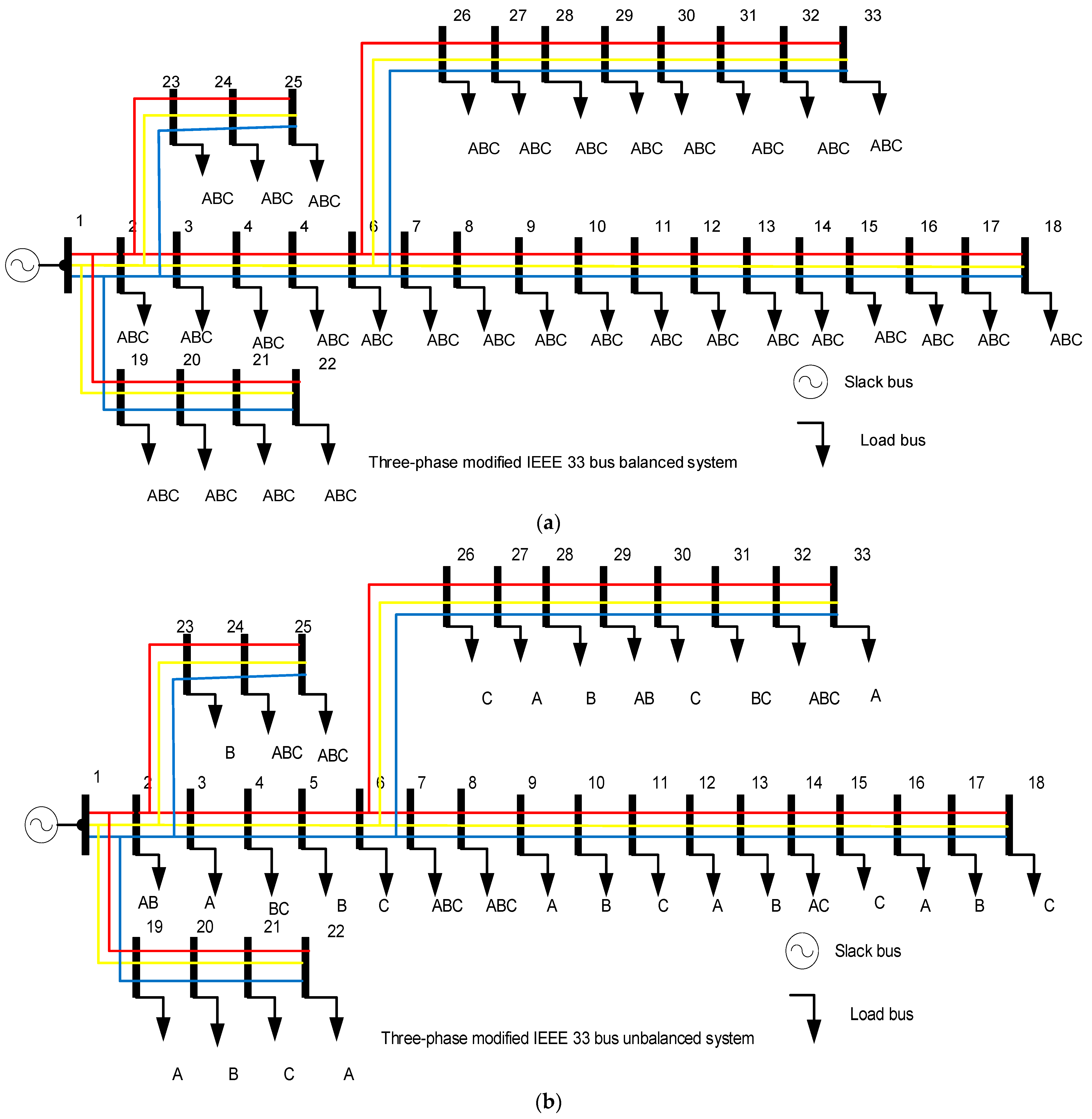
2.2. Three-Phase Distribution Networks
3. Modelling of Distribution Network
3.1. Modelling of Transmission Line
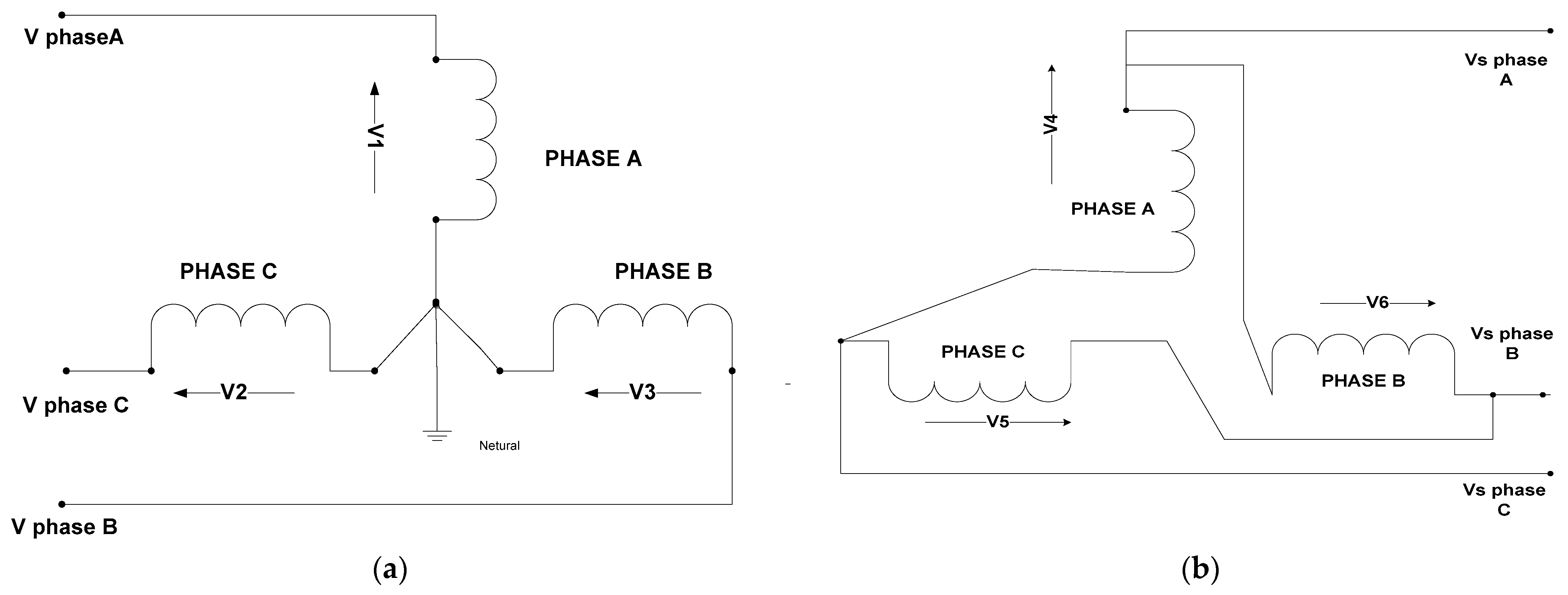
3.2. Modelling of Three-Phase Distribution Transformer
3.3. Distribution Load Flow Methodology
3.4. Constraint Considerations
3.4.1. Voltage Limit Constraints
3.4.2. DCER Active and Reactive Power Constraints
3.5. Performance Parameters
3.5.1. Active and Reactive Power Losses
3.5.2. Pollutant Emissions
3.5.3. Cost of Energy Loss ()
3.5.4. Distribution Clean Energy Resource Cost
- where and are the active and reactive powers of DCER,
- where , and .
3.5.5. Payback Year for DCER
3.5.6. Solar Model
3.5.7. Wind Model
4. Multi-Objective Performance Function
4.1. Active Power Loss Index ()
4.2. Reactive Power Loss Index ()
4.3. Voltage Deviation Index (VDI)
5. Soft Computing Techniques
5.1. Particle Swarm Optimization (PSO)
5.2. Teaching–Learning-Based Optimization
5.2.1. Phase I: Teaching Phase
5.2.2. Phase II: Learner Phase
5.3. JAYA Optimization Algorithm
5.4. Sine Cosine Optimization (SCO) Algorithm
5.5. RAO Optimization Algorithm
5.6. HBO Algorithm
5.6.1. Phase I: Digging Phase
5.6.2. Phase II: Honey Phase
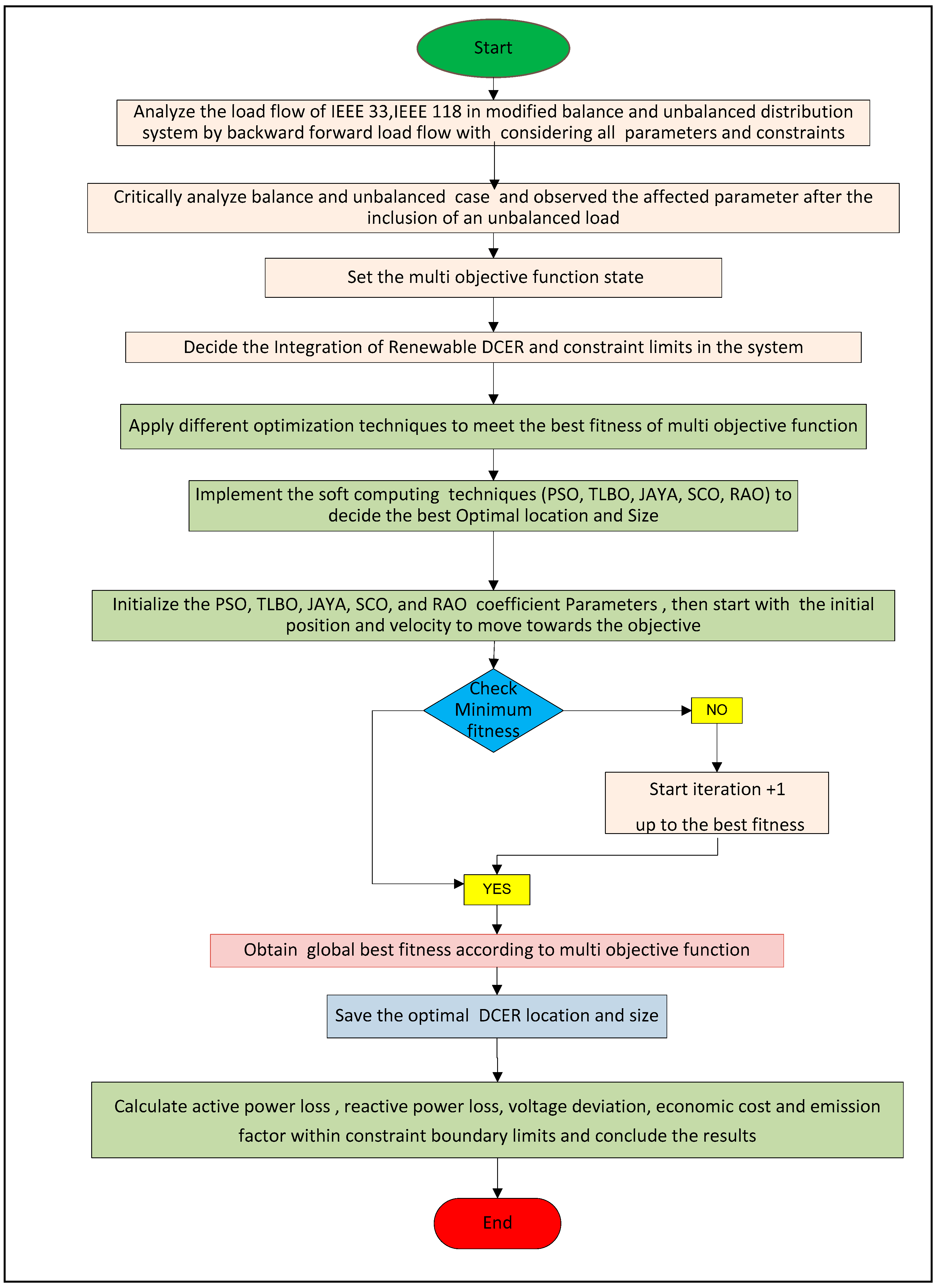
6. Results and Discussion
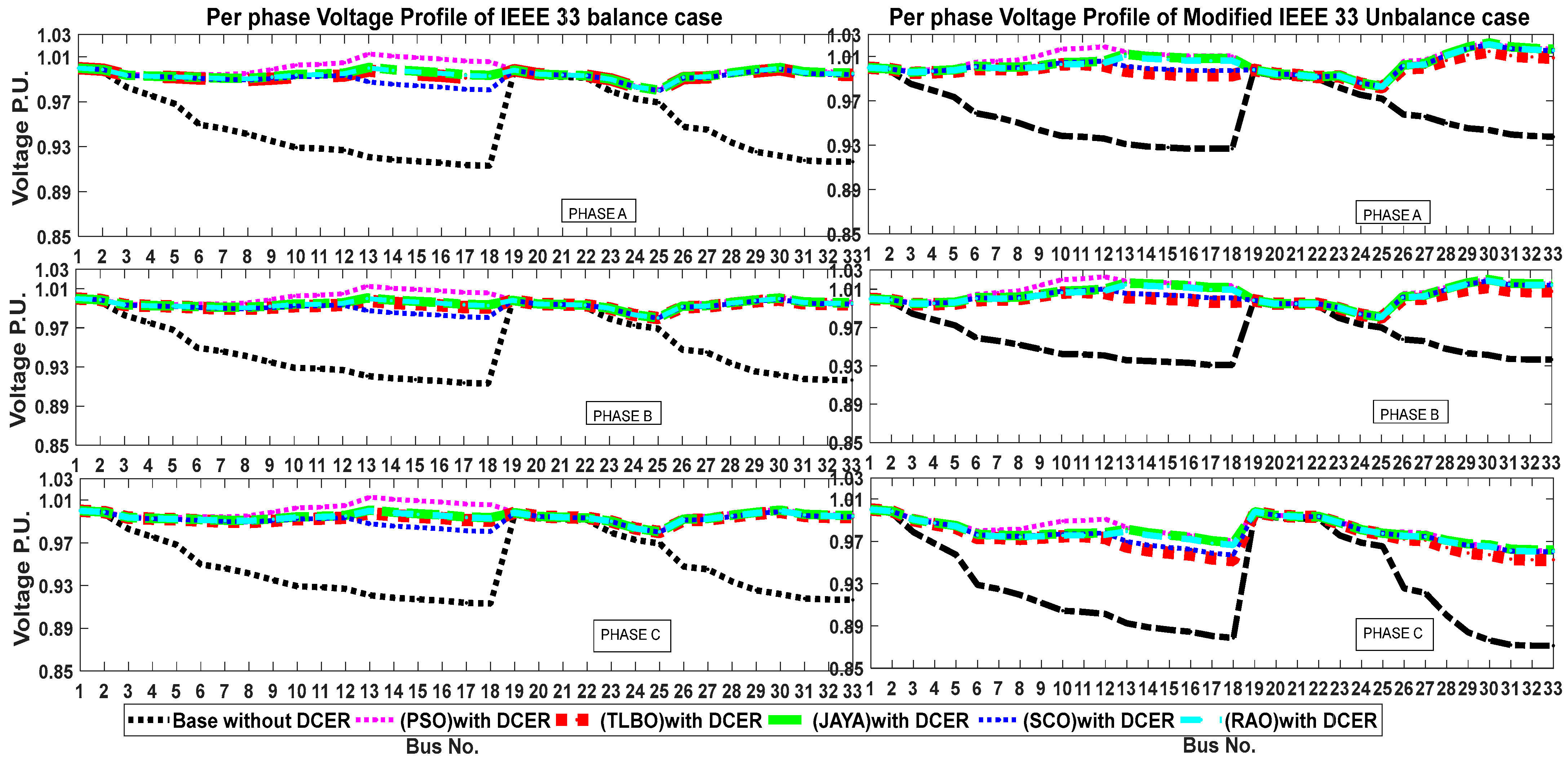
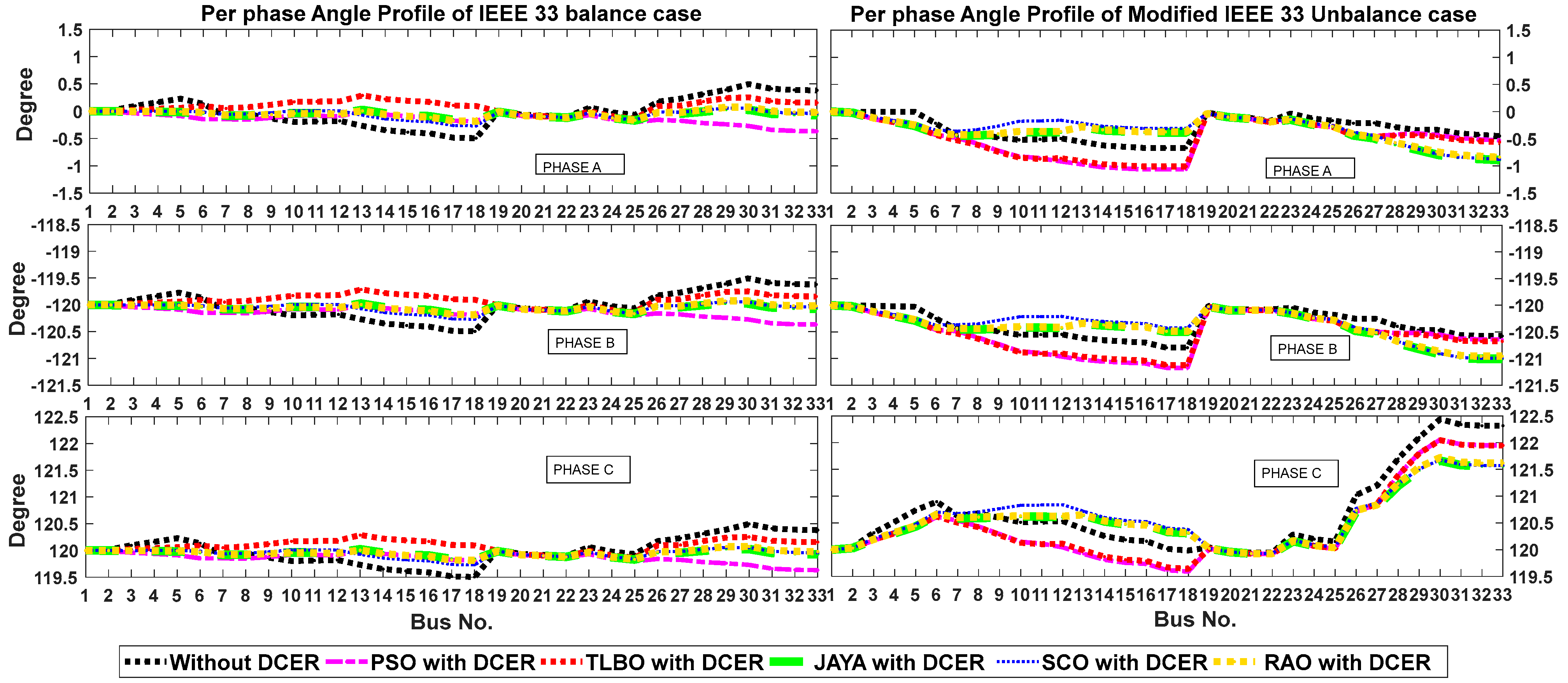
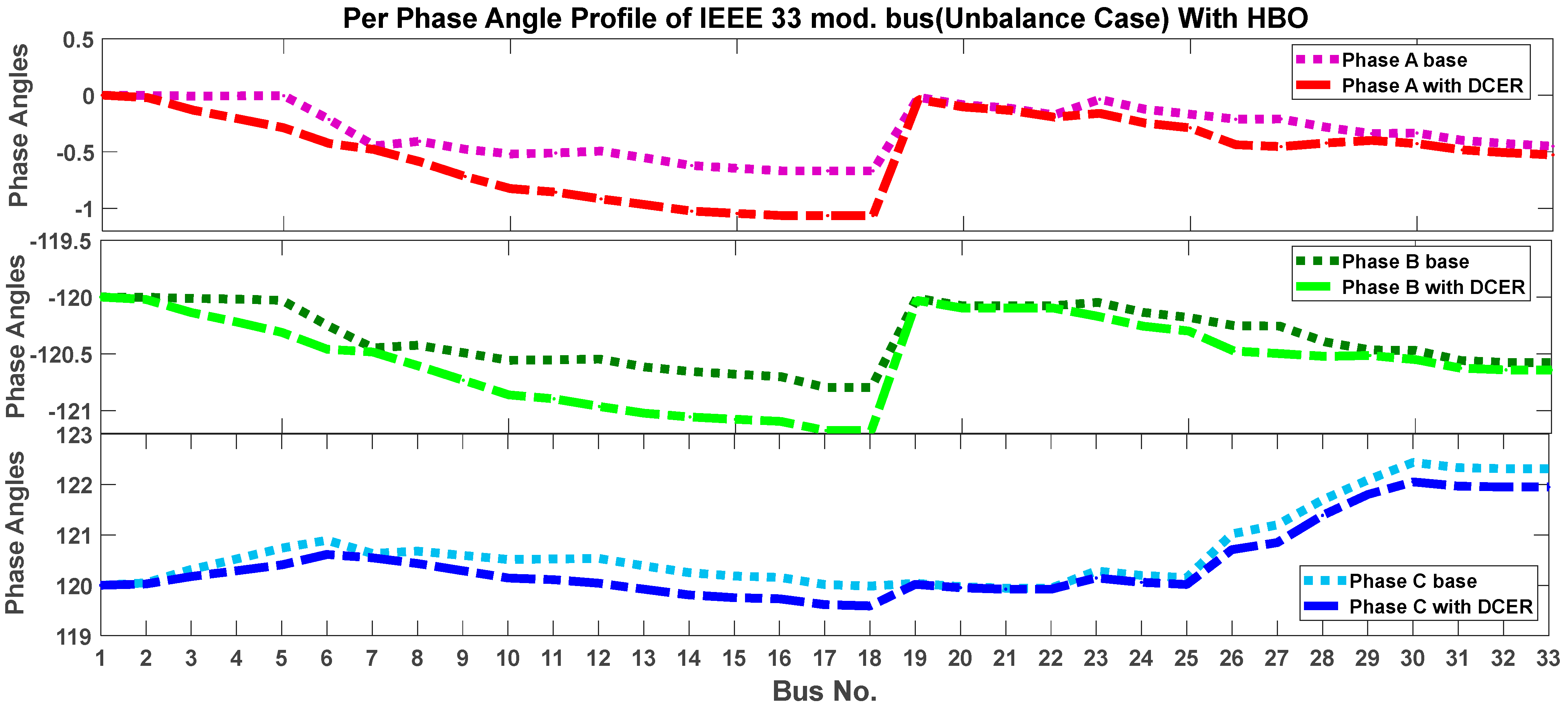
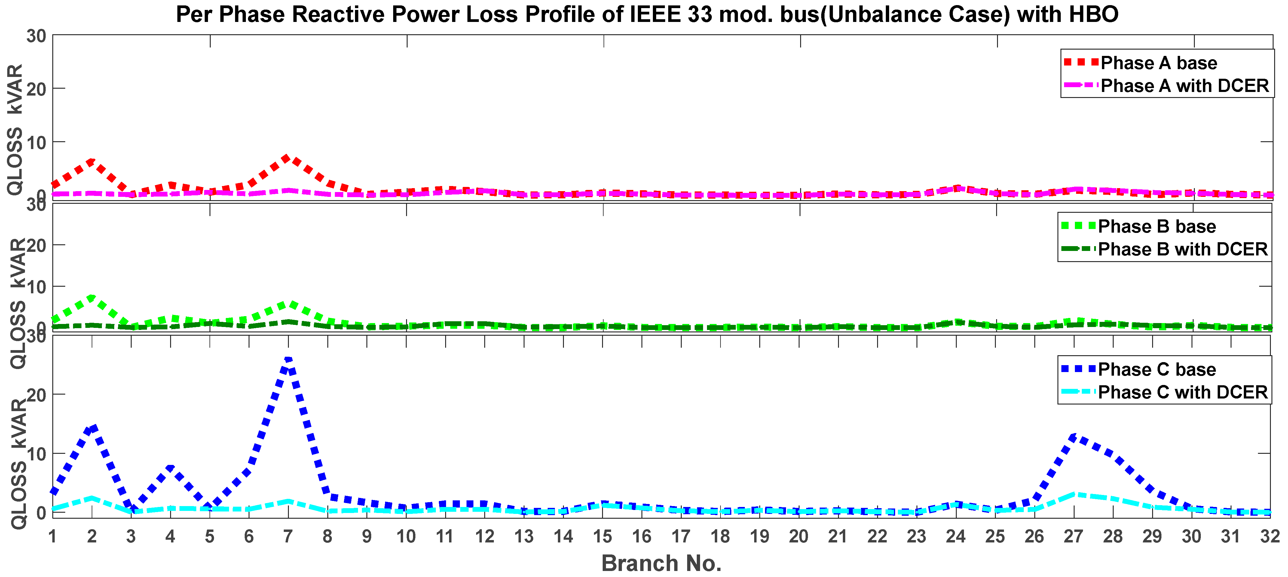
6.1. Case I: IEEE 33-Bus System
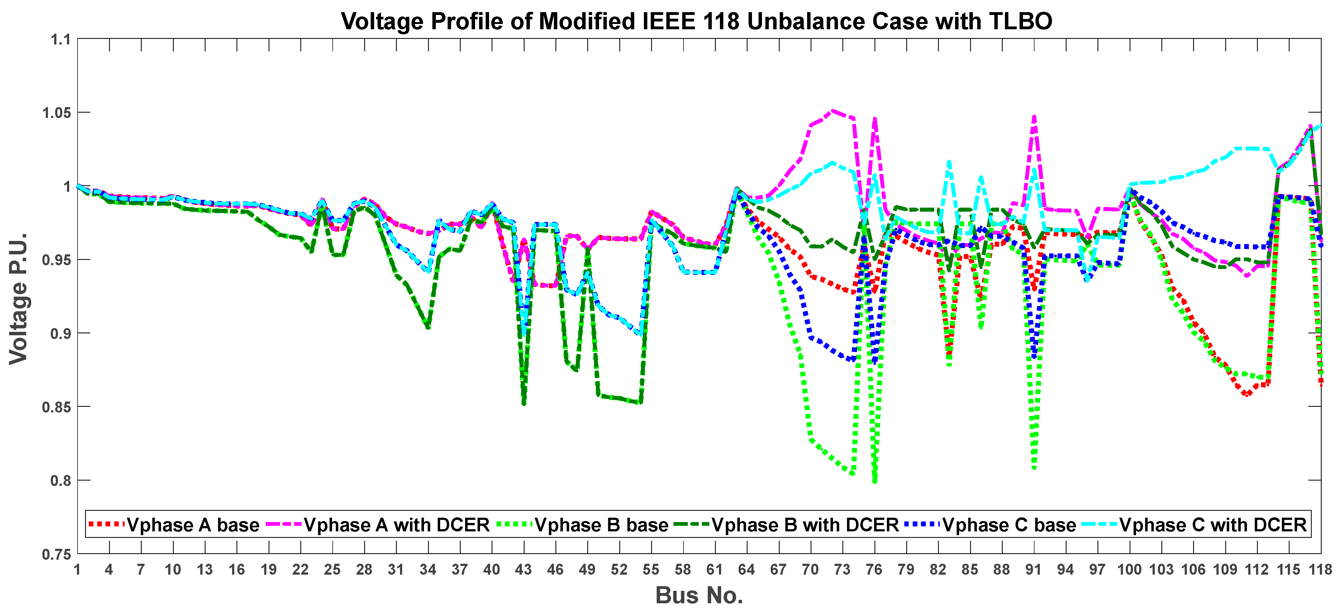
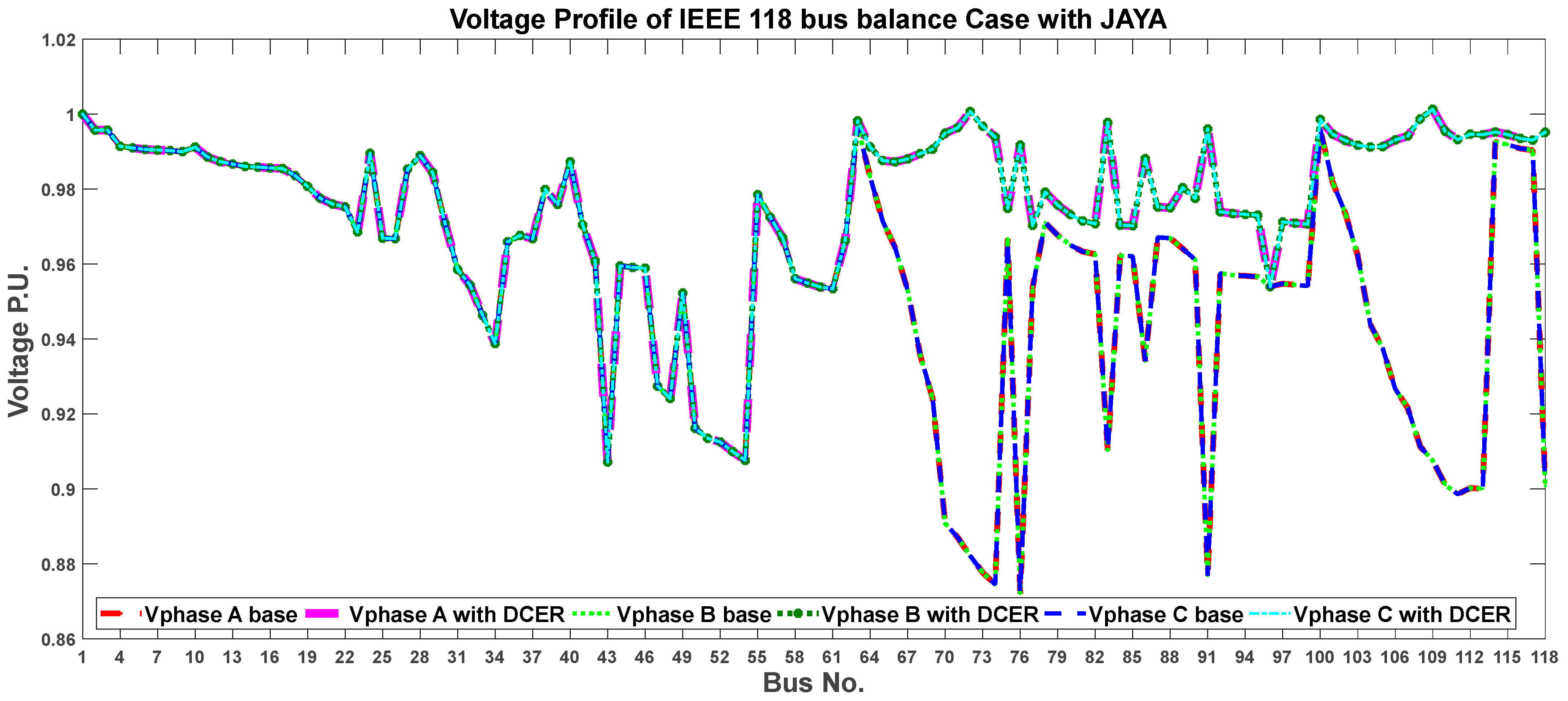
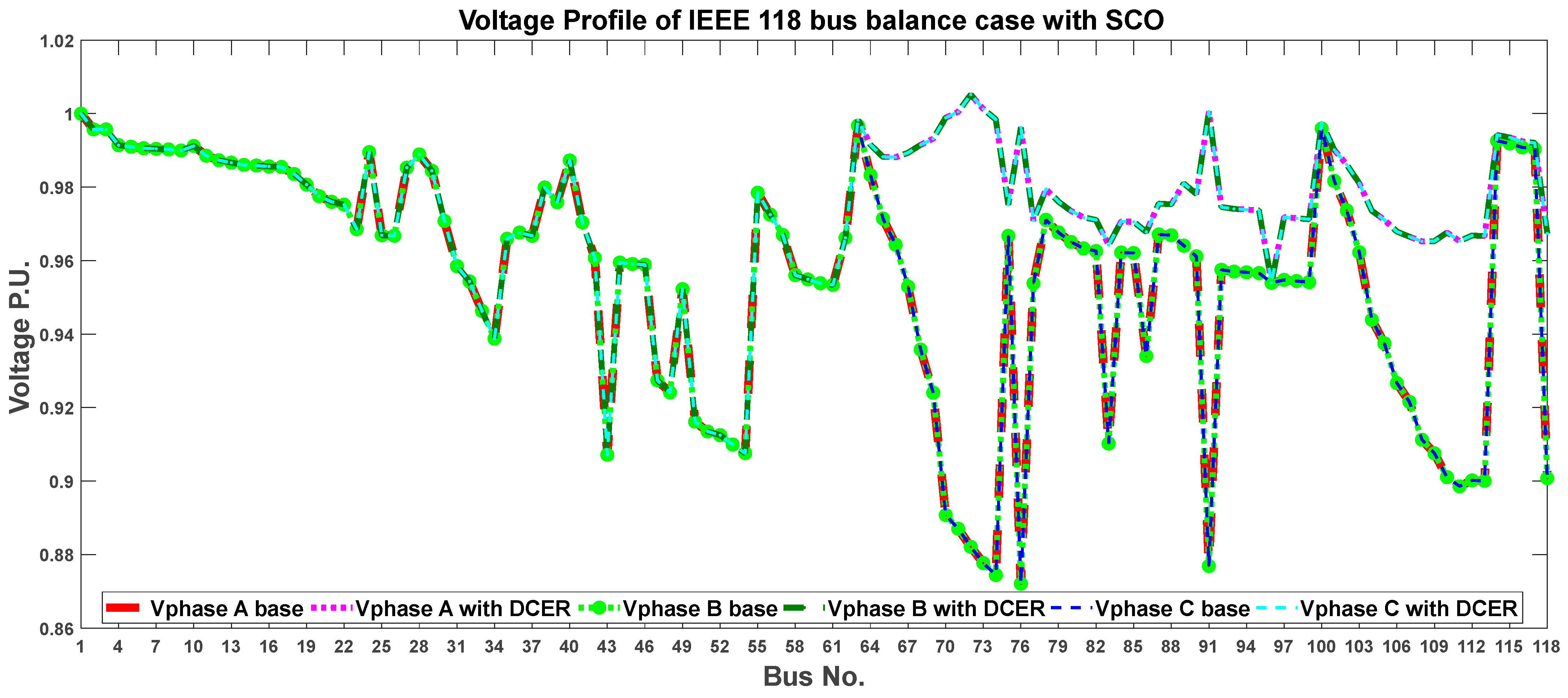
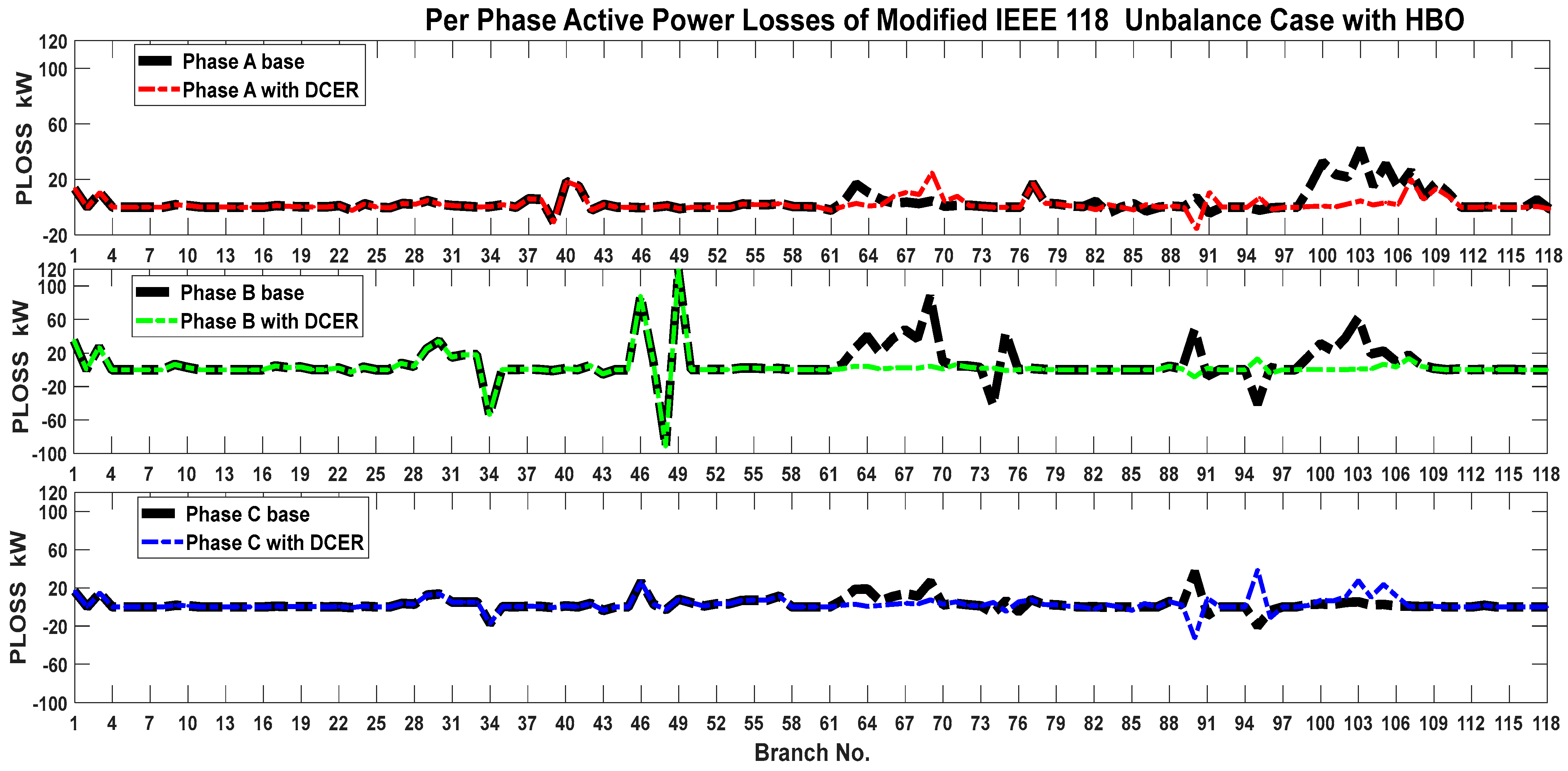
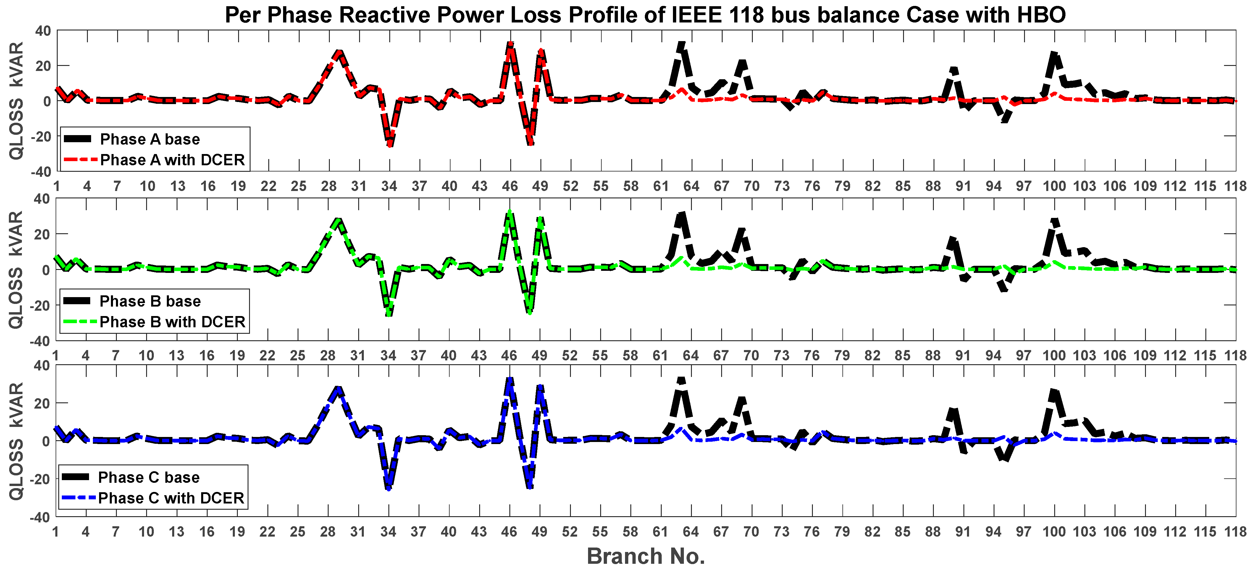
6.2. Case II: IEEE 118-Bus Distribution System
7. Conclusions
Author Contributions
Funding
Data Availability Statement
Acknowledgments
Conflicts of Interest
Abbreviations
| DCER | Distributed Clean Energy Resources |
| DG | Distribution Generation |
| PSO | Particle Swarm Optimization |
| TLBO | Teaching Learning-Based Optimization |
| SCO | Sine Cosine Optimization |
| KVL | Kirchhoff’s Voltage Law |
| KCL | Kirchhoff’s Current Law |
| NR | Newton Raphson |
| GHG | Greenhouse Gas |
| RAO | Rao Algorithm |
| RDN | Radial Distribution Network |
| HBO | Honey Badger Optimization |
| APSO | Adaptive Particle Swarm Optimization |
| MINLP | Mixed-Integer Nonlinear Programming |
| EHO | Elephant Herding Optimization |
| APLI | Active Power Loss Index |
| QPLI | Reactive Power Loss Index |
| VDI | Voltage Deviation Index |
| PFMO | Multi-Objective Performance Function |
| CEL | Cost of Energy Loss |
| JAYA | Jaya Algorithm |
| MOF | Multi-Objective Function |
| PFMO | Multi-Objective Performance Function |
Appendix A

| IEEE 33 Three-Phase Balanced Load Data | Modified IEEE 33 Unbalanced Three-Phase Load Data | ||||||||||||||||
|---|---|---|---|---|---|---|---|---|---|---|---|---|---|---|---|---|---|
| Bus No. | Phase Distribution | Connection Type | Bus Type | Active Load (Phase A) | Reactive Load (Phase A) | Active Load (Phase B) | Reactive Load (Phase B) | Active Load (Phase C) | Reactive Load (Phase C) | Phase Distribution | Connection Type | Active Load (Phase A) | Reactive Load (Phase A) | Active Load (Phase B) | Reactive Load (Phase B) | Active Load (Phase C) | Reactive Load (Phase C) |
| 1 | ABC | Y | slack | 0 | 0 | 0 | 0 | 0 | 0 | ABC | Y | 0 | 0 | 0 | 0 | 0 | 0 |
| 2 | ABC | Y | PQ | 33.33 | 20.00 | 33.33 | 20.00 | 33.33 | 20.00 | AB | Y | 50 | 30 | 50 | 30 | 0 | 0 |
| 3 | ABC | Y | PQ | 30.00 | 13.33 | 30.00 | 13.33 | 30.00 | 13.33 | A | Y | 90 | 40 | 0 | 0 | 0 | 0 |
| 4 | ABC | Y | PQ | 40.00 | 26.67 | 40.00 | 26.67 | 40.00 | 26.67 | BC | Y | 0 | 0 | 60 | 40 | 60 | 40 |
| 5 | ABC | Y | PQ | 20.00 | 10.00 | 20.00 | 10.00 | 20.00 | 10.00 | B | Y | 0 | 0 | 60 | 30 | 0 | 0 |
| 6 | ABC | Y | PQ | 20.00 | 6.67 | 20.00 | 6.67 | 20.00 | 6.67 | C | Y | 0 | 0 | 0 | 0 | 60 | 20 |
| 7 | ABC | Y | PQ | 66.67 | 33.33 | 66.67 | 33.33 | 66.67 | 33.33 | ABC | D | 66.67 | 33.33 | 66.67 | 33.33 | 66.67 | 33.33 |
| 8 | ABC | Y | PQ | 66.67 | 33.33 | 66.67 | 33.33 | 66.67 | 33.33 | ABC | Y | 66.67 | 33.33 | 66.67 | 33.33 | 66.67 | 33.33 |
| 9 | ABC | Y | PQ | 20.00 | 6.67 | 20.00 | 6.67 | 20.00 | 6.67 | A | Y | 60 | 20 | 0 | 0 | 0 | 0 |
| 10 | ABC | Y | PQ | 20.00 | 6.67 | 20.00 | 6.67 | 20.00 | 6.67 | B | Y | 0 | 0 | 60 | 20 | 0 | 0 |
| 11 | ABC | Y | PQ | 15.00 | 10.00 | 15.00 | 10.00 | 15.00 | 10.00 | C | Y | 0 | 0 | 0 | 0 | 45 | 30 |
| 12 | ABC | Y | PQ | 20.00 | 11.67 | 20.00 | 11.67 | 20.00 | 11.67 | A | Y | 60 | 35 | 0 | 0 | 0 | 0 |
| 13 | ABC | Y | PQ | 20.00 | 11.67 | 20.00 | 11.67 | 20.00 | 11.67 | B | Y | 0 | 0 | 60 | 35 | 0 | 0 |
| 14 | ABC | Y | PQ | 40.00 | 26.67 | 40.00 | 26.67 | 40.00 | 26.67 | AC | Y | 60 | 40 | 0 | 0 | 60 | 40 |
| 15 | ABC | Y | PQ | 20.00 | 3.33 | 20.00 | 3.33 | 20.00 | 3.33 | C | Y | 0 | 0 | 0 | 0 | 60 | 10 |
| 16 | ABC | Y | PQ | 20.00 | 6.67 | 20.00 | 6.67 | 20.00 | 6.67 | A | Y | 60 | 20 | 0 | 0 | 0 | 0 |
| 17 | ABC | Y | PQ | 20.00 | 6.67 | 20.00 | 6.67 | 20.00 | 6.67 | B | Y | 0 | 0 | 60 | 20 | 0 | 0 |
| 18 | ABC | Y | PQ | 30.00 | 13.33 | 30.00 | 13.33 | 30.00 | 13.33 | C | Y | 0 | 0 | 0 | 0 | 90 | 40 |
| 19 | ABC | Y | PQ | 30.00 | 13.33 | 30.00 | 13.33 | 30.00 | 13.33 | A | Y | 90 | 40 | 0 | 0 | 0 | 0 |
| 20 | ABC | Y | PQ | 30.00 | 13.33 | 30.00 | 13.33 | 30.00 | 13.33 | B | Y | 0 | 0 | 90 | 40 | 0 | 0 |
| 21 | ABC | Y | PQ | 30.00 | 13.33 | 30.00 | 13.33 | 30.00 | 13.33 | C | Y | 0 | 0 | 0 | 0 | 90 | 40 |
| 22 | ABC | Y | PQ | 30.00 | 13.33 | 30.00 | 13.33 | 30.00 | 13.33 | A | Y | 90 | 40 | 0 | 0 | 0 | 0 |
| 23 | ABC | Y | PQ | 30.00 | 16.67 | 30.00 | 16.67 | 30.00 | 16.67 | B | Y | 0 | 0 | 90 | 50 | 0 | 0 |
| 24 | ABC | Y | PQ | 140.00 | 66.67 | 140.00 | 66.67 | 140.00 | 66.67 | ABC | Y | 140 | 66.67 | 140 | 66.67 | 140 | 66.67 |
| 25 | ABC | Y | PQ | 140.00 | 66.67 | 140.00 | 66.67 | 140.00 | 66.67 | ABC | D | 140 | 66.67 | 140 | 66.67 | 140 | 66.67 |
| 26 | ABC | Y | PQ | 20.00 | 8.33 | 20.00 | 8.33 | 20.00 | 8.33 | C | Y | 0 | 0 | 0 | 0 | 60 | 25 |
| 27 | ABC | Y | PQ | 20.00 | 6.67 | 20.00 | 6.67 | 20.00 | 6.67 | A | Y | 60 | 25 | 0 | 0 | 0 | 0 |
| 28 | ABC | Y | PQ | 20.00 | 6.67 | 20.00 | 6.67 | 20.00 | 6.67 | B | Y | 0 | 0 | 60 | 20 | 0 | 0 |
| 29 | ABC | Y | PQ | 40.00 | 23.33 | 40.00 | 23.33 | 40.00 | 23.33 | AB | Y | 60 | 35 | 60 | 35 | 0 | 0 |
| 30 | ABC | Y | PQ | 66.67 | 200.00 | 66.67 | 200.00 | 66.67 | 200.00 | C | Y | 0 | 0 | 0 | 0 | 200 | 600 |
| 31 | ABC | Y | PQ | 50.00 | 23.33 | 50.00 | 23.33 | 50.00 | 23.33 | BC | Y | 0 | 0 | 75 | 35 | 75 | 35 |
| 32 | ABC | Y | PQ | 70.00 | 33.33 | 70.00 | 33.33 | 70.00 | 33.33 | ABC | Y | 70 | 33.33 | 70 | 33.33 | 70 | 33.33 |
| 33 | ABC | Y | PQ | 20.00 | 13.33 | 20.00 | 13.33 | 20.00 | 13.33 | A | Y | 60 | 40 | 0 | 0 | 0 | 0 |
Appendix B
| IEEE 118 Three-Phase Balanced Load Data | Modified IEEE 118 Unbalanced Three-Phase Load Data | ||||||||||||||||
|---|---|---|---|---|---|---|---|---|---|---|---|---|---|---|---|---|---|
| Bus No. | Phase Distribution | Connection Type | Bus Type | Active Load (Phase A) | Reactive Load (Phase A) | Active Load (Phase B) | Reactive Load (Phase B) | Active Load (Phase C) | Reactive Load (Phase C) | Phase Distribution | Connection Type | Active Load (Phase A) | Reactive Load (Phase A) | Active Load (Phase B) | Reactive Load (Phase B) | Active Load (Phase C) | Reactive Load (Phase C) |
| 1 | ABC | Y | slack | 0 | 0 | 0 | 0 | 0 | 0 | ABC | Y | 0.00 | 0.00 | 0.00 | 0.00 | 0.00 | 0.00 |
| 2 | ABC | Y | PQ | 44.61 | 33.71 | 44.61 | 33.71 | 44.61 | 33.71 | AB | Y | 66.92 | 50.57 | 66.92 | 50.57 | 0.00 | 0.00 |
| 3 | ABC | Y | PQ | 5.40 | 3.76 | 5.40 | 3.76 | 5.40 | 3.76 | A | Y | 16.21 | 11.29 | 0.00 | 0.00 | 0.00 | 0.00 |
| 4 | ABC | Y | PQ | 11.44 | 7.28 | 11.44 | 7.28 | 11.44 | 7.28 | BC | Y | 0.00 | 0.00 | 17.16 | 10.92 | 17.16 | 10.92 |
| 5 | ABC | Y | PQ | 24.34 | 21.20 | 24.34 | 21.20 | 24.34 | 21.20 | B | Y | 0.00 | 0.00 | 73.02 | 63.60 | 0.00 | 0.00 |
| 6 | ABC | Y | PQ | 48.07 | 22.87 | 48.07 | 22.87 | 48.07 | 22.87 | C | Y | 0.00 | 0.00 | 0.00 | 0.00 | 144.20 | 68.60 |
| 7 | ABC | Y | PQ | 34.82 | 20.58 | 34.82 | 20.58 | 34.82 | 20.58 | ABC | D | 34.82 | 20.58 | 34.82 | 20.58 | 34.82 | 20.58 |
| 8 | ABC | Y | PQ | 9.52 | 3.83 | 9.52 | 3.83 | 9.52 | 3.83 | ABC | Y | 9.52 | 3.83 | 9.52 | 3.83 | 9.52 | 3.83 |
| 9 | ABC | Y | PQ | 29.19 | 17.02 | 29.19 | 17.02 | 29.19 | 17.02 | A | Y | 87.56 | 51.07 | 0.00 | 0.00 | 0.00 | 0.00 |
| 10 | ABC | Y | PQ | 66.07 | 35.59 | 66.07 | 35.59 | 66.07 | 35.59 | B | Y | 0.00 | 0.00 | 198.20 | 106.77 | 0.00 | 0.00 |
| 11 | ABC | Y | PQ | 48.93 | 25.33 | 48.93 | 25.33 | 48.93 | 25.33 | C | Y | 0.00 | 0.00 | 0.00 | 0.00 | 146.80 | 76.00 |
| 12 | ABC | Y | PQ | 8.68 | 6.23 | 8.68 | 6.23 | 8.68 | 6.23 | A | Y | 26.04 | 18.69 | 0.00 | 0.00 | 0.00 | 0.00 |
| 13 | ABC | Y | PQ | 17.37 | 7.74 | 17.37 | 7.74 | 17.37 | 7.74 | B | Y | 0.00 | 0.00 | 52.10 | 23.22 | 0.00 | 0.00 |
| 14 | ABC | Y | PQ | 47.30 | 39.17 | 47.30 | 39.17 | 47.30 | 39.17 | AC | Y | 70.95 | 58.75 | 0.00 | 0.00 | 70.95 | 58.75 |
| 15 | ABC | Y | PQ | 7.29 | 9.60 | 7.29 | 9.60 | 7.29 | 9.60 | C | Y | 0.00 | 0.00 | 0.00 | 0.00 | 21.87 | 28.79 |
| 16 | ABC | Y | PQ | 11.12 | 8.82 | 11.12 | 8.82 | 11.12 | 8.82 | A | Y | 33.37 | 26.45 | 0.00 | 0.00 | 0.00 | 0.00 |
| 17 | ABC | Y | PQ | 10.81 | 8.41 | 10.81 | 8.41 | 10.81 | 8.41 | B | Y | 0.00 | 0.00 | 32.43 | 25.23 | 0.00 | 0.00 |
| 18 | ABC | Y | PQ | 6.74 | 3.97 | 6.74 | 3.97 | 6.74 | 3.97 | C | Y | 0.00 | 0.00 | 0.00 | 0.00 | 20.23 | 11.91 |
| 19 | ABC | Y | PQ | 52.31 | 26.17 | 52.31 | 26.17 | 52.31 | 26.17 | A | Y | 156.94 | 78.52 | 0.00 | 0.00 | 0.00 | 0.00 |
| 20 | ABC | Y | PQ | 182.10 | 117.13 | 182.10 | 117.13 | 182.10 | 117.13 | B | Y | 0.00 | 0.00 | 546.29 | 351.40 | 0.00 | 0.00 |
| 21 | ABC | Y | PQ | 60.10 | 54.73 | 60.10 | 54.73 | 60.10 | 54.73 | C | Y | 0.00 | 0.00 | 0.00 | 0.00 | 180.31 | 164.20 |
| 22 | ABC | Y | PQ | 31.06 | 18.20 | 31.06 | 18.20 | 31.06 | 18.20 | A | Y | 93.17 | 54.59 | 0.00 | 0.00 | 0.00 | 0.00 |
| 23 | ABC | Y | PQ | 28.39 | 13.22 | 28.39 | 13.22 | 28.39 | 13.22 | B | Y | 0.00 | 0.00 | 85.18 | 39.65 | 0.00 | 0.00 |
| 24 | ABC | Y | PQ | 56.03 | 31.73 | 56.03 | 31.73 | 56.03 | 31.73 | ABC | Y | 56.03 | 31.73 | 56.03 | 31.73 | 56.03 | 31.73 |
| 25 | ABC | Y | PQ | 41.70 | 50.07 | 41.70 | 50.07 | 41.70 | 50.07 | ABC | D | 41.70 | 50.07 | 41.70 | 50.07 | 41.70 | 50.07 |
| 26 | ABC | Y | PQ | 5.34 | 8.21 | 5.34 | 8.21 | 5.34 | 8.21 | C | Y | 0.00 | 0.00 | 0.00 | 0.00 | 16.03 | 24.62 |
| 27 | ABC | Y | PQ | 8.68 | 8.21 | 8.68 | 8.21 | 8.68 | 8.21 | A | Y | 26.03 | 24.62 | 0.00 | 0.00 | 0.00 | 0.00 |
| 28 | ABC | Y | PQ | 198.19 | 174.21 | 198.19 | 174.21 | 198.19 | 174.21 | B | Y | 0.00 | 0.00 | 594.56 | 522.62 | 0.00 | 0.00 |
| 29 | ABC | Y | PQ | 40.21 | 19.71 | 40.21 | 19.71 | 40.21 | 19.71 | AB | Y | 60.31 | 29.56 | 60.31 | 29.56 | 0.00 | 0.00 |
| 30 | ABC | Y | PQ | 34.13 | 33.18 | 34.13 | 33.18 | 34.13 | 33.18 | C | Y | 0.00 | 0.00 | 0.00 | 0.00 | 102.38 | 99.55 |
| 31 | ABC | Y | PQ | 171.13 | 106.17 | 171.13 | 106.17 | 171.13 | 106.17 | BC | Y | 0.00 | 0.00 | 256.70 | 159.25 | 256.70 | 159.25 |
| 32 | ABC | Y | PQ | 158.42 | 152.05 | 158.42 | 152.05 | 158.42 | 152.05 | ABC | Y | 158.42 | 152.05 | 158.42 | 152.05 | 158.42 | 152.05 |
| 33 | ABC | Y | PQ | 50.48 | 45.60 | 50.48 | 45.60 | 50.48 | 45.60 | A | Y | 151.43 | 136.79 | 0.00 | 0.00 | 0.00 | 0.00 |
| 34 | ABC | Y | PQ | 68.46 | 27.77 | 68.46 | 27.77 | 68.46 | 27.77 | ABC | Y | 68.46 | 27.77 | 68.46 | 27.77 | 68.46 | 27.77 |
| 35 | ABC | Y | PQ | 43.87 | 31.03 | 43.87 | 31.03 | 43.87 | 31.03 | AB | Y | 65.80 | 46.54 | 65.80 | 46.54 | 0.00 | 0.00 |
| 36 | ABC | Y | PQ | 149.47 | 123.26 | 149.47 | 123.26 | 149.47 | 123.26 | A | Y | 448.40 | 369.79 | 0.00 | 0.00 | 0.00 | 0.00 |
| 37 | ABC | Y | PQ | 146.84 | 107.21 | 146.84 | 107.21 | 146.84 | 107.21 | BC | Y | 0.00 | 0.00 | 220.26 | 160.82 | 220.26 | 160.82 |
| 38 | ABC | Y | PQ | 37.51 | 18.38 | 37.51 | 18.38 | 37.51 | 18.38 | B | Y | 0.00 | 0.00 | 112.54 | 55.13 | 0.00 | 0.00 |
| 39 | ABC | Y | PQ | 17.99 | 13.00 | 17.99 | 13.00 | 17.99 | 13.00 | C | Y | 0.00 | 0.00 | 0.00 | 0.00 | 53.96 | 39.00 |
| 40 | ABC | Y | PQ | 131.02 | 114.20 | 131.02 | 114.20 | 131.02 | 114.20 | ABC | D | 131.02 | 114.20 | 131.02 | 114.20 | 131.02 | 114.20 |
| 41 | ABC | Y | PQ | 108.91 | 92.85 | 108.91 | 92.85 | 108.91 | 92.85 | ABC | Y | 108.91 | 92.85 | 108.91 | 92.85 | 108.91 | 92.85 |
| 42 | ABC | Y | PQ | 178.75 | 80.08 | 178.75 | 80.08 | 178.75 | 80.08 | A | Y | 536.26 | 240.24 | 0.00 | 0.00 | 0.00 | 0.00 |
| 43 | ABC | Y | PQ | 25.42 | 22.19 | 25.42 | 22.19 | 25.42 | 22.19 | B | Y | 0.00 | 0.00 | 76.25 | 66.56 | 0.00 | 0.00 |
| 44 | ABC | Y | PQ | 17.84 | 13.25 | 17.84 | 13.25 | 17.84 | 13.25 | C | Y | 0.00 | 0.00 | 0.00 | 0.00 | 53.52 | 39.76 |
| 45 | ABC | Y | PQ | 13.44 | 10.65 | 13.44 | 10.65 | 13.44 | 10.65 | A | Y | 40.33 | 31.96 | 0.00 | 0.00 | 0.00 | 0.00 |
| 46 | ABC | Y | PQ | 13.22 | 6.92 | 13.22 | 6.92 | 13.22 | 6.92 | B | Y | 0.00 | 0.00 | 39.65 | 20.76 | 0.00 | 0.00 |
| 47 | ABC | Y | PQ | 22.07 | 14.12 | 22.07 | 14.12 | 22.07 | 14.12 | AC | Y | 33.10 | 21.18 | 0.00 | 0.00 | 33.10 | 21.18 |
| 48 | ABC | Y | PQ | 24.63 | 17.22 | 24.63 | 17.22 | 24.63 | 17.22 | C | Y | 0.00 | 0.00 | 0.00 | 0.00 | 73.90 | 51.65 |
| 49 | ABC | Y | PQ | 38.26 | 19.32 | 38.26 | 19.32 | 38.26 | 19.32 | A | Y | 114.77 | 57.97 | 0.00 | 0.00 | 0.00 | 0.00 |
| 50 | ABC | Y | PQ | 306.12 | 401.70 | 306.12 | 401.70 | 306.12 | 401.70 | B | Y | 0.00 | 0.00 | 918.37 | 1205.10 | 0.00 | 0.00 |
| 51 | ABC | Y | PQ | 70.10 | 48.89 | 70.10 | 48.89 | 70.10 | 48.89 | C | Y | 0.00 | 0.00 | 0.00 | 0.00 | 210.30 | 146.66 |
| 52 | ABC | Y | PQ | 22.23 | 18.87 | 22.23 | 18.87 | 22.23 | 18.87 | A | Y | 66.68 | 56.61 | 0.00 | 0.00 | 0.00 | 0.00 |
| 53 | ABC | Y | PQ | 14.07 | 13.39 | 14.07 | 13.39 | 14.07 | 13.39 | B | Y | 0.00 | 0.00 | 42.21 | 40.18 | 0.00 | 0.00 |
| 54 | ABC | Y | PQ | 144.58 | 94.47 | 144.58 | 94.47 | 144.58 | 94.47 | C | Y | 0.00 | 0.00 | 0.00 | 0.00 | 433.74 | 283.41 |
| 55 | ABC | Y | PQ | 20.70 | 8.95 | 20.70 | 8.95 | 20.70 | 8.95 | A | Y | 62.10 | 26.86 | 0.00 | 0.00 | 0.00 | 0.00 |
| 56 | ABC | Y | PQ | 30.82 | 29.46 | 30.82 | 29.46 | 30.82 | 29.46 | B | Y | 0.00 | 0.00 | 92.46 | 88.38 | 0.00 | 0.00 |
| 57 | ABC | Y | PQ | 28.40 | 18.48 | 28.40 | 18.48 | 28.40 | 18.48 | ABC | Y | 28.40 | 18.48 | 28.40 | 18.48 | 28.40 | 18.48 |
| 58 | ABC | Y | PQ | 115.10 | 110.80 | 115.10 | 110.80 | 115.10 | 110.80 | ABC | D | 115.10 | 110.80 | 115.10 | 110.80 | 115.10 | 110.80 |
| 59 | ABC | Y | PQ | 7.50 | 5.61 | 7.50 | 5.61 | 7.50 | 5.61 | C | Y | 0.00 | 0.00 | 0.00 | 0.00 | 22.50 | 16.83 |
| 60 | ABC | Y | PQ | 26.85 | 16.39 | 26.85 | 16.39 | 26.85 | 16.39 | A | Y | 80.55 | 49.16 | 0.00 | 0.00 | 0.00 | 0.00 |
| 61 | ABC | Y | PQ | 31.95 | 30.25 | 31.95 | 30.25 | 31.95 | 30.25 | B | Y | 0.00 | 0.00 | 95.86 | 90.76 | 0.00 | 0.00 |
| 62 | ABC | Y | PQ | 20.97 | 15.90 | 20.97 | 15.90 | 20.97 | 15.90 | AB | Y | 31.46 | 23.85 | 31.46 | 23.85 | 0.00 | 0.00 |
| 63 | ABC | Y | PQ | 159.60 | 154.58 | 159.60 | 154.58 | 159.60 | 154.58 | C | Y | 0.00 | 0.00 | 0.00 | 0.00 | 478.80 | 463.74 |
| 64 | ABC | Y | PQ | 40.31 | 17.34 | 40.31 | 17.34 | 40.31 | 17.34 | BC | Y | 0.00 | 0.00 | 60.47 | 26.00 | 60.47 | 26.00 |
| 65 | ABC | Y | PQ | 46.37 | 33.45 | 46.37 | 33.45 | 46.37 | 33.45 | ABC | Y | 46.37 | 33.45 | 46.37 | 33.45 | 46.37 | 33.45 |
| 66 | ABC | Y | PQ | 130.59 | 64.50 | 130.59 | 64.50 | 130.59 | 64.50 | A | Y | 391.78 | 193.50 | 0.00 | 0.00 | 0.00 | 0.00 |
| 67 | ABC | Y | PQ | 9.25 | 8.90 | 9.25 | 8.90 | 9.25 | 8.90 | ABC | Y | 9.25 | 8.90 | 9.25 | 8.90 | 9.25 | 8.90 |
| 68 | ABC | Y | PQ | 17.60 | 8.42 | 17.60 | 8.42 | 17.60 | 8.42 | AB | Y | 26.41 | 12.63 | 26.41 | 12.63 | 0.00 | 0.00 |
| 69 | ABC | Y | PQ | 22.30 | 12.90 | 22.30 | 12.90 | 22.30 | 12.90 | A | Y | 66.89 | 38.71 | 0.00 | 0.00 | 0.00 | 0.00 |
| 70 | ABC | Y | PQ | 155.83 | 131.71 | 155.83 | 131.71 | 155.83 | 131.71 | BC | Y | 0.00 | 0.00 | 233.75 | 197.57 | 233.75 | 197.57 |
| 71 | ABC | Y | PQ | 198.28 | 79.91 | 198.28 | 79.91 | 198.28 | 79.91 | B | Y | 0.00 | 0.00 | 594.85 | 239.74 | 0.00 | 0.00 |
| 72 | ABC | Y | PQ | 44.17 | 28.12 | 44.17 | 28.12 | 44.17 | 28.12 | C | Y | 0.00 | 0.00 | 0.00 | 0.00 | 132.50 | 84.36 |
| 73 | ABC | Y | PQ | 17.57 | 7.49 | 17.57 | 7.49 | 17.57 | 7.49 | ABC | D | 17.57 | 7.49 | 17.57 | 7.49 | 17.57 | 7.49 |
| 74 | ABC | Y | PQ | 289.93 | 204.93 | 289.93 | 204.93 | 289.93 | 204.93 | ABC | Y | 289.93 | 204.93 | 289.93 | 204.93 | 289.93 | 204.93 |
| 75 | ABC | Y | PQ | 10.45 | 9.94 | 10.45 | 9.94 | 10.45 | 9.94 | A | Y | 31.35 | 29.82 | 0.00 | 0.00 | 0.00 | 0.00 |
| 76 | ABC | Y | PQ | 64.13 | 40.81 | 64.13 | 40.81 | 64.13 | 40.81 | B | Y | 0.00 | 0.00 | 192.39 | 122.43 | 0.00 | 0.00 |
| 77 | ABC | Y | PQ | 21.92 | 15.12 | 21.92 | 15.12 | 21.92 | 15.12 | C | Y | 0.00 | 0.00 | 0.00 | 0.00 | 65.75 | 45.37 |
| 78 | ABC | Y | PQ | 79.38 | 74.41 | 79.38 | 74.41 | 79.38 | 74.41 | A | Y | 238.15 | 223.22 | 0.00 | 0.00 | 0.00 | 0.00 |
| 79 | ABC | Y | PQ | 98.18 | 54.16 | 98.18 | 54.16 | 98.18 | 54.16 | B | Y | 0.00 | 0.00 | 294.55 | 162.47 | 0.00 | 0.00 |
| 80 | ABC | Y | PQ | 161.86 | 145.97 | 161.86 | 145.97 | 161.86 | 145.97 | AC | Y | 242.79 | 218.96 | 0.00 | 0.00 | 242.79 | 218.96 |
| 81 | ABC | Y | PQ | 81.18 | 61.01 | 81.18 | 61.01 | 81.18 | 61.01 | C | Y | 0.00 | 0.00 | 0.00 | 0.00 | 243.53 | 183.03 |
| 82 | ABC | Y | PQ | 81.18 | 61.01 | 81.18 | 61.01 | 81.18 | 61.01 | A | Y | 243.53 | 183.03 | 0.00 | 0.00 | 0.00 | 0.00 |
| 83 | ABC | Y | PQ | 44.75 | 39.76 | 44.75 | 39.76 | 44.75 | 39.76 | B | Y | 0.00 | 0.00 | 134.25 | 119.29 | 0.00 | 0.00 |
| 84 | ABC | Y | PQ | 7.57 | 9.32 | 7.57 | 9.32 | 7.57 | 9.32 | C | Y | 0.00 | 0.00 | 0.00 | 0.00 | 22.71 | 27.96 |
| 85 | ABC | Y | PQ | 16.50 | 8.84 | 16.50 | 8.84 | 16.50 | 8.84 | A | Y | 49.51 | 26.52 | 0.00 | 0.00 | 0.00 | 0.00 |
| 86 | ABC | Y | PQ | 127.93 | 85.72 | 127.93 | 85.72 | 127.93 | 85.72 | B | Y | 0.00 | 0.00 | 383.78 | 257.16 | 0.00 | 0.00 |
| 87 | ABC | Y | PQ | 16.55 | 6.87 | 16.55 | 6.87 | 16.55 | 6.87 | C | Y | 0.00 | 0.00 | 0.00 | 0.00 | 49.64 | 20.60 |
| 88 | ABC | Y | PQ | 7.49 | 3.94 | 7.49 | 3.94 | 7.49 | 3.94 | A | Y | 22.47 | 11.81 | 0.00 | 0.00 | 0.00 | 0.00 |
| 89 | ABC | Y | PQ | 20.98 | 14.32 | 20.98 | 14.32 | 20.98 | 14.32 | B | Y | 0.00 | 0.00 | 62.93 | 42.96 | 0.00 | 0.00 |
| 90 | ABC | Y | PQ | 10.22 | 11.64 | 10.22 | 11.64 | 10.22 | 11.64 | ABC | Y | 10.22 | 11.64 | 10.22 | 11.64 | 10.22 | 11.64 |
| 91 | ABC | Y | PQ | 20.84 | 22.26 | 20.84 | 22.26 | 20.84 | 22.26 | ABC | D | 20.84 | 22.26 | 20.84 | 22.26 | 20.84 | 22.26 |
| 92 | ABC | Y | PQ | 38.19 | 27.25 | 38.19 | 27.25 | 38.19 | 27.25 | C | Y | 0.00 | 0.00 | 0.00 | 0.00 | 114.57 | 81.75 |
| 93 | ABC | Y | PQ | 27.10 | 22.18 | 27.10 | 22.18 | 27.10 | 22.18 | A | Y | 81.29 | 66.53 | 0.00 | 0.00 | 0.00 | 0.00 |
| 94 | ABC | Y | PQ | 10.58 | 5.32 | 10.58 | 5.32 | 10.58 | 5.32 | B | Y | 0.00 | 0.00 | 31.73 | 15.96 | 0.00 | 0.00 |
| 95 | ABC | Y | PQ | 11.11 | 20.16 | 11.11 | 20.16 | 11.11 | 20.16 | AB | Y | 16.66 | 30.24 | 16.66 | 30.24 | 0.00 | 0.00 |
| 96 | ABC | Y | PQ | 177.09 | 74.95 | 177.09 | 74.95 | 177.09 | 74.95 | C | Y | 0.00 | 0.00 | 0.00 | 0.00 | 531.28 | 224.85 |
| 97 | ABC | Y | PQ | 169.01 | 122.47 | 169.01 | 122.47 | 169.01 | 122.47 | BC | Y | 0.00 | 0.00 | 253.52 | 183.71 | 253.52 | 183.71 |
| 98 | ABC | Y | PQ | 8.80 | 3.90 | 8.80 | 3.90 | 8.80 | 3.90 | ABC | Y | 8.80 | 3.90 | 8.80 | 3.90 | 8.80 | 3.90 |
| 99 | ABC | Y | PQ | 15.33 | 10.13 | 15.33 | 10.13 | 15.33 | 10.13 | A | Y | 45.99 | 30.39 | 0.00 | 0.00 | 0.00 | 0.00 |
| 100 | ABC | Y | PQ | 33.55 | 15.86 | 33.55 | 15.86 | 33.55 | 15.86 | ABC | Y | 33.55 | 15.86 | 33.55 | 15.86 | 33.55 | 15.86 |
| 101 | ABC | Y | PQ | 152.16 | 116.77 | 152.16 | 116.77 | 152.16 | 116.77 | AB | Y | 228.24 | 175.15 | 228.24 | 175.15 | 0.00 | 0.00 |
| 102 | ABC | Y | PQ | 174.19 | 149.76 | 174.19 | 149.76 | 174.19 | 149.76 | A | Y | 522.56 | 449.29 | 0.00 | 0.00 | 0.00 | 0.00 |
| 103 | ABC | Y | PQ | 136.14 | 56.15 | 136.14 | 56.15 | 136.14 | 56.15 | BC | Y | 0.00 | 0.00 | 204.22 | 84.23 | 204.22 | 84.23 |
| 104 | ABC | Y | PQ | 47.16 | 44.75 | 47.16 | 44.75 | 47.16 | 44.75 | B | Y | 0.00 | 0.00 | 141.48 | 134.25 | 0.00 | 0.00 |
| 105 | ABC | Y | PQ | 34.81 | 22.01 | 34.81 | 22.01 | 34.81 | 22.01 | C | Y | 0.00 | 0.00 | 0.00 | 0.00 | 104.43 | 66.02 |
| 106 | ABC | Y | PQ | 32.26 | 27.88 | 32.26 | 27.88 | 32.26 | 27.88 | ABC | D | 32.26 | 27.88 | 32.26 | 27.88 | 32.26 | 27.88 |
| 107 | ABC | Y | PQ | 164.64 | 139.78 | 164.64 | 139.78 | 164.64 | 139.78 | ABC | Y | 164.64 | 139.78 | 164.64 | 139.78 | 164.64 | 139.78 |
| 108 | ABC | Y | PQ | 75.13 | 45.29 | 75.13 | 45.29 | 75.13 | 45.29 | A | Y | 225.38 | 135.88 | 0.00 | 0.00 | 0.00 | 0.00 |
| 109 | ABC | Y | PQ | 169.74 | 129.07 | 169.74 | 129.07 | 169.74 | 129.07 | B | Y | 0.00 | 0.00 | 509.21 | 387.21 | 0.00 | 0.00 |
| 110 | ABC | Y | PQ | 62.83 | 57.82 | 62.83 | 57.82 | 62.83 | 57.82 | C | Y | 0.00 | 0.00 | 0.00 | 0.00 | 188.50 | 173.46 |
| 111 | ABC | Y | PQ | 306.01 | 299.52 | 306.01 | 299.52 | 306.01 | 299.52 | A | Y | 918.03 | 898.55 | 0.00 | 0.00 | 0.00 | 0.00 |
| 112 | ABC | Y | PQ | 101.69 | 71.79 | 101.69 | 71.79 | 101.69 | 71.79 | B | Y | 0.00 | 0.00 | 305.08 | 215.37 | 0.00 | 0.00 |
| 113 | ABC | Y | PQ | 18.13 | 13.66 | 18.13 | 13.66 | 18.13 | 13.66 | AC | Y | 27.19 | 20.49 | 0.00 | 0.00 | 27.19 | 20.49 |
| 114 | ABC | Y | PQ | 70.38 | 64.30 | 70.38 | 64.30 | 70.38 | 64.30 | C | Y | 0.00 | 0.00 | 0.00 | 0.00 | 211.14 | 192.90 |
| 115 | ABC | Y | PQ | 22.34 | 17.78 | 22.34 | 17.78 | 22.34 | 17.78 | A | Y | 67.01 | 53.34 | 0.00 | 0.00 | 0.00 | 0.00 |
| 116 | ABC | Y | PQ | 54.02 | 30.11 | 54.02 | 30.11 | 54.02 | 30.11 | B | Y | 0.00 | 0.00 | 162.07 | 90.32 | 0.00 | 0.00 |
| 117 | ABC | Y | PQ | 16.26 | 9.72 | 16.26 | 9.72 | 16.26 | 9.72 | C | Y | 0.00 | 0.00 | 0.00 | 0.00 | 48.79 | 29.16 |
| 118 | ABC | Y | PQ | 11.30 | 6.33 | 11.30 | 6.33 | 11.30 | 6.33 | A | Y | 33.90 | 18.98 | 0.00 | 0.00 | 0.00 | 0.00 |
References
- Das, D.; Kothari, D.P.; Kalam, A. Simple and efficient method for load flow solution of radial distribution networks. Int. J. Electr. Power Energy Syst. 1995, 17, 335–346. [Google Scholar] [CrossRef]
- Haque, M.H. Load flow solution of distribution systems with voltage-dependent load models. Electr. Power Syst. Res. 1996, 36, 151–156. [Google Scholar] [CrossRef]
- Bohre, A.K.; Agnihotri, G.; Dubey, M. Optimal sizing and sitting of DG with load models using soft computing techniques in practical distribution system. IET Gener. Transm. Distrib. 2016, 10, 2606–2621. [Google Scholar] [CrossRef]
- Hu, Z.; Wang, X. A probabilistic load flow method considering branch outages. IEEE Trans. Power Syst. 2006, 21, 507–514. [Google Scholar] [CrossRef]
- Das, B. Consideration of input parameter uncertainties in load flow solution of three-phase unbalanced radial distribution system. IEEE Trans. Power Syst. 2006, 21, 1088–1095. [Google Scholar] [CrossRef]
- Vieira, J.C.M.; Freitas, W.; Morelato, A. Phase-decoupled method for three-phase power-flow analysis of unbalanced distribution systems. IEE Proc.-Gener. Transm. Distrib. 2004, 151, 568–574. [Google Scholar] [CrossRef]
- Li, L.; Zhizhong, G.; Chengmin, W. A new topology structure and load flow solution for radial distribution networks. In Proceedings of the International Conference on Power System Technology, Kunming, China, 13–17 October 2002; Volume 2, pp. 1064–1067. [Google Scholar]
- Rani, K.S.; Acharjee, P.; Bohre, A.K. Determining Optimal Size and Placement of Renewable DG Considering Variation of Load. Blue Eyes Intell. Eng. Sci. 2019, 8, 310–315. [Google Scholar] [CrossRef]
- Bohre, A.K.; Agnihotri, G.; Dubey, M. The optimal distributed generation placement sizing using novel optimization technique. Middle-East. J. Sci. Res 2015, 10, 1228–1236. [Google Scholar]
- Rani, K.S.; Saw, B.K.; Achargee, P.; Bohre, A.K. Optimal sizing and placement of renewable DGs using GOA considering seasonal variation of load and DGs. In Proceedings of the 2020 International Conference on Computational Intelligence for Smart Power System and Sustainable Energy (CISPSSE), Keonjhar, India, 29–31 July 2020; pp. 1–6. [Google Scholar]
- Bohre, A.K.; Agnihotri, G.; Dubey, M.; Kalambe, S. Impacts of the Load Models on Optimal Planning of Distributed Generation in Distribution System. Adv. Artif. Intell. 2015, 2015, 297436. [Google Scholar] [CrossRef]
- Kalesar, B.M.; Seifi, A.R. Fuzzy load flow in balanced and unbalanced radial distribution systems incorporating composite load model. Int. J. Electr. Power Energy Syst. 2010, 32, 17–23. [Google Scholar] [CrossRef]
- Nayak, M.R.; Behura, D.; Nayak, S. Performance analysis of unbalanced radial feeder for integrating energy storage system with wind generator using inherited competitive swarm optimization algorithm. J. Energy Storage 2021, 38, 102574. [Google Scholar] [CrossRef]
- Daratha, N.; Das, B.; Sharma, J. Robust voltage regulation in unbalanced radial distribution system under uncertainty of distributed generation and loads. Int. J. Electr. Power Energy Syst. 2015, 73, 516–527. [Google Scholar] [CrossRef]
- Raju, G.V.; Bijwe, P.R. Reactive power/voltage control in distribution systems under uncertain environment. IET Gener. Transm. Distrib. 2008, 2, 752–763. [Google Scholar] [CrossRef]
- Su, C.L. Stochastic evaluation of voltages in distribution networks with distributed generation using detailed distribution operation models. IEEE Trans. Power Syst. 2009, 25, 786–795. [Google Scholar] [CrossRef]
- Prasad, C.H.; Subbaramaiah, K.; Sujatha, P. Cost–benefit analysis for optimal DG placement in distribution systems by using elephant herding optimization algorithm. Renew. Wind. Water Sol. 2019, 6, 2. [Google Scholar] [CrossRef]
- Yammani, C.; Maheswarapu, S.; Matam, S.K. A Multi-objective Shuffled Bat algorithm for optimal placement and sizing of multi distributed generations with different load models. Int. J. Electr. Power Energy Syst. 2016, 79, 120–131. [Google Scholar] [CrossRef]
- Suresh, M.C.V.; Belwin, E.J. Optimal DG placement for benefit maximization in distribution networks by using Dragonfly algorithm. Renew. Wind. Water Sol. 2018, 5, 4. [Google Scholar] [CrossRef]
- Murty, V.V.; Kumar, A. Optimal placement of DG in radial distribution systems based on new voltage stability index under load growth. Int. J. Electr. Power Energy Syst. 2015, 69, 246–256. [Google Scholar] [CrossRef]
- Dashtdar, M.; Najafi, M.; Esmaeilbeig, M.; Bajaj, M. Placement and optimal size of DG in the distribution network based on nodal pricing reduction with nonlinear load model using the IABC algorithm. Sādhanā 2022, 47, 73. [Google Scholar] [CrossRef]
- Dolatabadi, S.H.; Ghorbanian, M.; Siano, P.; Hatziargyriou, N.D. An Enhanced IEEE 33 Bus Benchmark Test System for Distribution System Studies. IEEE Trans. Power Syst. 2020, 36, 2565–2572. [Google Scholar] [CrossRef]
- Bohre, A.K.; Agnihotri, G.; Dubey, M.; Kalambe, S. Assessment of Intericate DG Planning With Practical Load Models by using PSO. Electr. Comput. Eng. Int. J. (ECIJ) 2015, 4, 15–22. [Google Scholar] [CrossRef]
- Bohre, A.K.; Acharjee, P.; Sawle, Y. Analysis of grid connected hybrid micro-grid with different utility tariffs. In Proceedings of the 2021 1st International Conference on Power Electronics and Energy (ICPEE), Bhubaneswar, India, 2–3 January 2021; pp. 1–6. [Google Scholar]
- Kansal, S. Cost-Benefit analysis for Optimal DG Placement in Distribution Systems. Int. J. Ambient. Energy 2015, 38, 45–54. [Google Scholar] [CrossRef]
- Mtonga, T.P.; Kaberere, K.K.; Irungu, G.K. Optimal network reconfiguration for real power losses reduction in the IEEE 33-bus radial distribution system. In Proceedings of the 2022 Sustainable Research and Innovation (SRI) Conference, Nairobi, Kenya, 5–6 October 2022. [Google Scholar]
- Vempalle, R.; Kumar, D.P. An intelligent optimization technique for performance improvement in radial distribution network. Int. J. Intell. Unmanned Syst. 2022, 52. [Google Scholar] [CrossRef]
- Xie, X.; Sun, Y. A piecewise probabilistic harmonic power flow approach in unbalanced residential distribution systems. Int. J. Electr. Power Energy Syst. 2022, 141, 108114. [Google Scholar] [CrossRef]
- Antić, T.; Thurner, L.; Capuder, T.; Pavić, I. Modeling and open source implementation of balanced and unbalanced harmonic analysis in radial distribution networks. Electr. Power Syst. Res. 2022, 209, 107935. [Google Scholar] [CrossRef]
- Arrilliaga, J.; Bradley, D.A.; Bodger, P.S. Power System Harmonics; Wiley: Hoboken, NJ, USA, 1985. [Google Scholar]
- Yan, Y.H.; Chen, C.S.; Moo, C.S.; Hsu, C.T. Harmonic analysis for industrial customers. IEEE Trans. Ind. Appl. Soc. 1994, 30, 462–468. [Google Scholar] [CrossRef]
- Kennedy, J.; Eberhart, R. Particle swarm optimization. In Proceedings of the ICNN’95-International Conference on Neural Networks, Perth, Australia, 17 November–1 December 1995; Volume 4, pp. 1942–1948. [Google Scholar]
- Rao, R.V. Teaching-learning-based optimization algorithm. In Teaching Learning Based Optimization Algorithm; Springer: Cham, Switzerland, 2016; pp. 9–39. [Google Scholar]
- Rao, R.V.; Savsani, V.J.; Balic, J. Teaching–learning-based optimization algorithm for unconstrained and constrained real-parameter optimization problems. Eng. Optim. 2012, 44, 1447–1462. [Google Scholar] [CrossRef]
- Rao, R.V.; Savsani, V.J.; Vakharia, D.P. Teaching–learning-based optimization: A novel method for constrained mechanical design optimization problems. Comput.-Aided Des. 2011, 43, 303–315. [Google Scholar] [CrossRef]
- Rao, R. Jaya: A simple and new optimization algorithm for solving constrained and unconstrained optimization problems. Int. J. Ind. Eng. Comput. 2016, 7, 19–34. [Google Scholar]
- Mirjalili, S. SCA: A sine cosine algorithm for solving optimization problems. Knowl.-Based Syst. 2016, 96, 120–133. [Google Scholar] [CrossRef]
- Rao, R.V.; Keesari, H.S. Rao algorithms for multi-objective optimization of selected thermodynamic cycles. Eng. Comput. 2021, 37, 3409–3437. [Google Scholar] [CrossRef]
- Rao, R. Rao algorithms: Three metaphor-less simple algorithms for solving optimization problems. Int. J. Ind. Eng. Comput. 2020, 11, 107–130. [Google Scholar] [CrossRef]
- William, H.K. Distribution System Modelling and Analysis; CRC Press: Boca Raton, FL, USA, 2012. [Google Scholar]
- Abdelhay, A.S.; Om, P.M. Electric Distribution Systems; Wiley: Hoboken, NJ, USA, 2011. [Google Scholar]
- Chen, T.-H.; Chen, M.-S.; Inoue, T.; Kotas, P.; Chebli, E.A. Three-phase co-generator and transformer models for distribution system analysis. IEEE Trans. Power Deliv. 1991, 6, 1671–1681. [Google Scholar] [CrossRef]
- Teng, J.H.; Chang, C.Y. A novel and fast three-phase load flow for unbalanced radial distribution systems. IEEE Trans. Power Syst. 2002, 17, 1238–1244. [Google Scholar] [CrossRef]
- Milovanović, M.; Radosavljević, J.; Arsić, N.; Perović, B. A Power Flow Method for Unbalanced Three-Phase Distribution Networks with Nonlinear Loads. In Proceedings of the 2022 21st International Symposium INFOTEH-JAHORINA (INFOTEH), East Sarajevo, Bosnia and Herzegovina, 16–18 March 2022; pp. 1–6. [Google Scholar] [CrossRef]
- Emanuel, A.E. Summary of IEEE standard 1459: Definitions for the measurement of electric power quantities under sinusoidal, non-sinusoidal, balanced, or unbalanced conditions. IEEE Trans. Ind. Appl. 2004, 40, 869–876. [Google Scholar] [CrossRef]
- Meena, N.K.; Swarnkar, A.; Gupta, N.; Niazi, K.R. Multi-objective Taguchi approach for optimal DG integration in distribution systems. IET Gener. Transm. Distrib. 2017, 11, 2418–2428. [Google Scholar] [CrossRef]
- Singh, P.; Meena, N.K.; Yang, J.; Vega-Fuentes, E.; Bishnoi, S.K. Multi-criteria decision making monarch butterfly optimization for optimal distributed energy resources mix in distribution networks. Appl. Energy 2020, 278, 115723. [Google Scholar] [CrossRef]
- HOMER® Energy. HOMER Grid, Version 1.8 User Manual; HOMER® Energy: Boulder, CO, USA. Available online: https://support.ul-renewables.com/homer-manual-grid/index.html (accessed on 12 December 2023).
- Wang, C. Modeling and Control of Hybrid Wind/Photovoltaic/Fuel Cell Distributed Generation Systems. Ph.D. Thesis, Montana State University, Bozeman, MT, USA, 2006. [Google Scholar]
- Adewumi, O.B.; Fotis, G.; Vita, V.; Nankoo, D.; Ekonomou, L. The impact of distributed energy storage on distribution and transmission networks’ power quality. Appl. Sci. 2022, 12, 6466. [Google Scholar] [CrossRef]
- Liu, B.; Braslavsky, J.H. Robust dynamic operating envelopes for DER integration in unbalanced distribution networks. IEEE Trans. Power Syst. 2023, 39, 3921–3936. [Google Scholar] [CrossRef]
- Pinthurat, W.; Hredzak, B.; Konstantinou, G.; Fletcher, J. Techniques for compensation of unbalanced conditions in LV distribution networks with integrated renewable generation: An overview. Electr. Power Syst. Res. 2023, 214, 108932. [Google Scholar] [CrossRef]
- Zhang, D.; Shafiullah, G.M.; Das, C.K.; Wong, K.W. Optimal Allocation of Battery Energy Storage Systems to Enhance System Performance and Reliability in Unbalanced Distribution Networks. Energies 2023, 16, 7127. [Google Scholar] [CrossRef]
- Jiao, W.; Wu, Q.; Huang, S.; Chen, J.; Li, C.; Zhou, B. DMPC based distributed voltage control for unbalanced distribution networks with single-/three-phase DGs. Int. J. Electr. Power Energy Syst. 2023, 150, 109068. [Google Scholar] [CrossRef]
- Vijayan, V.; Mohapatra, A.; Singh, S.N.; Dewangan, C.L. An Efficient Modular Optimization Scheme for Unbalanced Active Distribution Networks with uncertain EV and PV Penetrations. IEEE Trans. Smart Grid 2023, 14, 3876–3888. [Google Scholar] [CrossRef]
- Yang, N.C.; Liu, M.J.; Lai, K.Y.; Adinda, E.W. Three-phase power flow calculations using initial voltage estimation method for unbalanced distribution networks. IEEE Access 2022, 10, 103705–103717. [Google Scholar] [CrossRef]
- Tapia-Tinoco, G.; Granados-Lieberman, D.; Valtierra-Rodriguez, M.; Avina-Cervantes, J.G.; Garcia-Perez, A. Modeling of electric springs and their multi-objective voltage control based on continuous genetic algorithm for unbalanced distribution networks. Int. J. Electr. Power Energy Syst. 2022, 138, 107979. [Google Scholar] [CrossRef]
- Zandrazavi, S.F.; Guzman, C.P.; Pozos, A.T.; Quiros-Tortos, J.; Franco, J.F. Stochastic multi-objective optimal energy management of grid-connected unbalanced microgrids with renewable energy generation and plug-in electric vehicles. Energy 2022, 241, 122884. [Google Scholar] [CrossRef]
- Lotfi, H.; Ghazi, R. Optimal participation of demand response aggregators in reconfigurable distribution system considering photovoltaic and storage units. J. Ambient Intell. Humaniz. Comput. 2021, 12, 2233–2255. [Google Scholar] [CrossRef]
- Lotfi, H. Multi-objective energy management approach in distribution grid integrated with energy storage units considering the demand response program. Int. J. Energy Res. 2020, 44, 10662–10681. [Google Scholar] [CrossRef]
- Lotfi, H. Optimal sizing of distributed generation units and shunt capacitors in the distribution system considering uncertainty resources by the modified evolutionary algorithm. J. Ambient Intell. Humaniz. Comput. 2022, 13, 4739–4758. [Google Scholar] [CrossRef]
- Mondal, S.; De, M. Distributed Energy Resource Deployment to Mitigate Adverse Effects of High EV Penetration in Unbalanced Distribution System by Analytical Sensitivity-Based Optimization. Electr. Power Compon. Syst. 2024, 2024, 1–12. [Google Scholar] [CrossRef]
- Mondal, S.; De, M. Optimal capacitor placement for unbalanced distribution system using graph theory. IETE J. Res. 2023, 69, 6512–6519. [Google Scholar] [CrossRef]
- El-Sehiemy, R.; Shaheen, A.; Ginidi, A.; Elhosseini, M. A Honey Badger Optimization for Minimizing the Pollutant Environmental Emissions-Based Economic Dispatch Model Integrating Combined Heat and Power Units. Energies 2022, 15, 7603. [Google Scholar] [CrossRef]
- Hashim, F.A.; Houssein, E.H.; Hussain, K.; Mabrouk, M.S.; Al-Atabany, W. Honey Badger Algorithm: New metaheuristic algorithm for solving optimization problems. Math. Comput. Simul. 2022, 192, 84–110. [Google Scholar] [CrossRef]
- Aljohani, T.M.; Saad, A.; Mohammed, O.A. Two-stage optimization strategy for solving the VVO problem considering high penetration of plug-in electric vehicles to unbalanced distribution networks. IEEE Trans. Ind. Appl. 2021, 57, 3425–3440. [Google Scholar] [CrossRef]
- Girigoudar, K.; Roald, L.A. On the impact of different voltage unbalance metrics in distribution system optimization. Electr. Power Syst. Res. 2020, 189, 106656. [Google Scholar] [CrossRef]
- Mousavi, M.; Wu, M. A DSO framework for market participation of DER aggregators in unbalanced distribution networks. IEEE Trans. Power Syst. 2021, 37, 2247–2258. [Google Scholar] [CrossRef]
- Barutcu, I.C.; Karatepe, E.; Boztepe, M. Impact of harmonic limits on PV penetration levels in unbalanced distribution networks considering load and irradiance uncertainty. Int. J. Electr. Power Energy Syst. 2020, 118, 105780. [Google Scholar] [CrossRef]
- Zheng, W.; Huang, W.; Hill, D.J. A deep learning-based general robust method for network reconfiguration in three-phase unbalanced active distribution networks. Int. J. Electr. Power Energy Syst. 2020, 120, 105982. [Google Scholar] [CrossRef]
- Hashmi, M.U.; Koirala, A.; Ergun, H.; Van Hertem, D. Flexible and curtailable resource activation in three-phase unbalanced distribution networks. Electr. Power Syst. Res. 2022, 212, 108608. [Google Scholar] [CrossRef]
- Rafi, F.H.M.; Hossain, M.J.; Rahman, M.S.; Taghizadeh, S. An overview of unbalance compensation techniques using power electronic converters for active distribution systems with renewable generation. Renew. Sustain. Energy Rev. 2020, 125, 109812. [Google Scholar] [CrossRef]
- Guo, Y.; Zhang, Q.; Wang, Z. Cooperative peak shaving and voltage regulation in unbalanced distribution feeders. IEEE Trans. Power Syst. 2021, 36, 5235–5244. [Google Scholar] [CrossRef]
- Mohamed, M.A.E.H.; Ali, Z.M.; Ahmed, M.; Al-Gahtani, S.F. Energy saving maximization of balanced and unbalanced distribution power systems via network reconfiguration and optimum capacitor allocation using a hybrid metaheuristic algorithm. Energies 2021, 14, 3205. [Google Scholar] [CrossRef]
- Souheyla, B.; Omar, B. Golden Jackal Algorithm for Optimal Size and Location of Distributed Generation in Unbalanced Distribution Networks. Alger. J. Renew. Energy Sustain. Dev. 2023, 5, 28–39. [Google Scholar]
- Dincer, F. The analysis on photovoltaic electricity generation status, potential and policies of the leading countries in solar energy. Renew. Sustain. Energy Rev. 2011, 15, 713–720. [Google Scholar] [CrossRef]
- Kumar, V.; Shrivastava, R.L.; Untawale, S.P. Solar energy: Review of potential green & clean energy for coastal and offshore applications. Aquat. Procedia 2015, 4, 473–480. [Google Scholar]
- Fathi, R.; Tousi, B.; Galvani, S. A new approach for optimal allocation of photovoltaic and wind clean energy resources in distribution networks with reconfiguration considering uncertainty based on info-gap decision theory with risk aversion strategy. J. Clean. Prod. 2021, 295, 125984. [Google Scholar] [CrossRef]
- Tarhan, C.; Çil, M.A. A study on hydrogen, the clean energy of the future: Hydrogen storage methods. J. Energy Storage 2021, 40, 102676. [Google Scholar] [CrossRef]
- Ismail, B.I. Power Generation Using Nonconventional Renewable Geothermal & Alternative Clean Energy Technologies. In Planet Earth 2011: Global Warming Challenges and Opportunities for Policy and Practice; IntechOpen: London, UK, 2011. [Google Scholar]
- Surendra, K.C.; Takara, D.; Hashimoto, A.G.; Khanal, S.K. Biogas as a sustainable energy source for developing countries: Opportunities and challenges. Renew. Sustain. Energy Rev. 2014, 31, 846–859. [Google Scholar] [CrossRef]
- Ouali, S.; Cherkaoui, A. An improved backward/forward sweep power flow method based on a new network information organization for radial distribution systems. J. Electr. Comput. Eng. 2020, 2020, 5643410. [Google Scholar] [CrossRef]
- Hossain, E.; Tür, M.R.; Padmanaban, S.; Ay, S.; Khan, I. Analysis and mitigation of power quality issues in distributed generation systems using custom power devices. IEEE Access 2018, 6, 16816–16833. [Google Scholar] [CrossRef]
- Ha, M.P.; Huy, P.D.; Ramachandaramurthy, V.K. A review of the optimal allocation of distributed generation: Objectives, constraints, methods, and algorithms. Renew. Sustain. Energy Rev. 2017, 75, 293–312. [Google Scholar]
- Rawat, M.S.; Vadhera, S. Probabilistic approach to determine penetration of hybrid renewable DGs in distribution network based on voltage stability index. Arab. J. Sci. Eng. 2020, 45, 1473–1498. [Google Scholar] [CrossRef]
- Abido, M.A. Optimal power flow using particle swarm optimization. Int. J. Electr. Power Energy Syst. 2002, 24, 563–571. [Google Scholar] [CrossRef]
- Hester, R.E.; Harrison, R.M. Air pollution in the 21st century. J. Chem. Technol. Biotechnol. 2007, 82, 731–742. [Google Scholar]
- Ghasemian, S.; Faridzad, A.; Abbaszadeh, P.; Taklif, A.; Ghasemi, A.; Hafezi, R. An overview of global energy scenarios by 2040: Identifying the driving forces using cross-impact analysis method. Int. J. Environ. Sci. Technol. 2020, 21, 1–24. [Google Scholar] [CrossRef]
- Rao, R.S.; Ravindra, K.; Satish, K.; Narasimham, S.V.L. Power loss minimization in distribution system using network reconfiguration in the presence of distributed generation. IEEE Trans. Power Syst. 2012, 28, 317–325. [Google Scholar] [CrossRef]
- Kansal, S.; Kumar, V.; Tyagi, B. Composite active and reactive power compensation of distribution networks. In Proceedings of the 2012 IEEE 7th International Conference on Industrial and Information Systems (ICIIS), Chennai, India, 6–9 August 2012; pp. 1–6. [Google Scholar]
- Zhu, J.Z. Optimal reconfiguration of electrical distribution network using the refined genetic algorithm. Electr. Power Syst. Res. 2002, 62, 37–42. [Google Scholar] [CrossRef]
- Gopiya-Naik, S.; Khatod, D.K.; Sharma, M.P. Optimal allocation of distributed generation in distribution system for loss reduction. In Proceedings of the 2012 IACSIT Coimbatore Conferences, Coimbatore, India, 18–19 February 2012; Volume 28, pp. 42–46. [Google Scholar]


| Author(s) | Bus System | Objective | Methodology | Outcomes |
|---|---|---|---|---|
| Das, D. et al. [1] | Radial distribution network (RDN) | To solve load flow problems for RDNs. | The proposed method solely focuses on evaluating the voltage magnitudes using basic algebraic expressions. | RDN load flow solution is a simple and efficient method. |
| Bohre, A.K. et al. [3] | Standard balanced IEEE 33, IEEE 54, and IEEE 69 RDNs | To find optimal DG sizing and placement using load models and soft computing approaches. | Optimal solution for an MOF is obtained using GA and PSO. | Proposed method offers economic benefits, enhanced reliability, and minimized losses. |
| Hu, Z. and Wang, X. [4] | The 24-bus RDN | To solve load flow using the probabilistic load flow technique with branch outages taken into account. | Probabilistic load flow method. | Proposed load flow approach can perform faster speed calculations that consider branch outages. |
| Rani, K. et al. [8] | Practical balanced 94-bus system | Optimal size and placement of renewable DG with load variation. | Solved by APSO. | Voltage index, active power loss, and cost-economic factor improvements were suggested. |
| Kalesar, B.M. and Seifi, A.R. [12] | Balanced and unbalanced RDNs | Composite load model with fuzzy load flow. | Fuzzy load flow method. | The results showed that this fuzzy load flow method can be used in large-scale balanced and unbalanced distribution systems. |
| Nayak, M.R. et al. [13] | IEEE 37 unbalanced RDN | Optimal allocation of BESS energy with wind power penetrations. | Inherited Competitive Swarm Optimization. | Showed a suitable sustainable average charging method to charge the battery, reduce the loss, and enhance the voltage profile. |
| Daratha, N. et al. [14] | Modified IEEE 123 unbalanced RDN | To fix the voltage regulation issue in unbalanced RDNs. | Problem solved by mixed-integer nonlinear programming (MINLP) and Monte Carlo simulations to obtain optimal result. | The results show that, even in the presence of generation and load uncertainties, the magnitude and imbalance ratio of voltages will always remain within the specified limits. |
| Suresh, M.C.V. and Belwin, E.J. [19] | IEEE 15, 33, and 69 balanced RDNs | To improve voltage profile, regulation, losses, and stability, and minimize the cost. | Dragonfly algorithm used for minimization of objective function and the results were compared with those of the Elephant Herding Optimization Algorithm and evolutionary algorithms. | Results showed a reduction in losses and cost using proposed method. |
| Murty, V.V. and Kumar, A. [20] | IEEE 12, modified 12, IEEE 69 and IEEE 85 bus | To decide on the best DG placement based on the revised voltage stability index. | Proposed voltage stability index method. | The proposed methodology showed an enhancement of voltage stability of the system under load growth. |
| Dashtdar, M. et al. [21] | 38-bus RDN | To determine DG placement and appropriate size based on reducing nodal pricing using a nonlinear load model. | Improved Artificial Bee Colony (IABC) algorithm for optimization. | Showed a reduction in nodal pricing and indices of loss. |
| Mtonga, T.P. et al. [26] | IEEE 33 bus and IEEE 69-bus balanced RDNs | Reconfiguration of network. | Sparrow search algorithm. | Reduced real power losses and enhanced the efficiency and performance. |
| Xie, X. and Sun, Y. [28] | IEEE-13, 123, and 8500 tests | To analyse the probabilistic and time-varying harmonics. | Developed method for evaluating harmonic characteristics in unbalanced residential distribution systems. | Evaluated the probabilistic harmonic emission level. |
| Teng, J.H. and Chang, C.Y. [43] | Unbalanced RDN | To develop a novel and fast three-phase load flow method. | Proposed a unique and fast three-phase load flow approach for imbalanced RDNs. | The approach enhanced the efficiency and speed of load flow calculations. |
| Milovanović, M. et al. [44] | IEEE 13 unbalanced RDN | To develop a power flow method for nonlinear loads. | Introduced a power flow approach for nonlinear loads in unbalanced three-phase distribution networks. | Showed improved accuracy in analysing systems with nonlinear load components. |
| Meena, N.K. et al. [46] | Distribution systems | To find optimal integration of DG into distribution systems. | Multi-objective Taguchi approach (MOTA). | Optimal integration of DG and improved system performance and reliability. |
| Singh, P. et al. [47] | IEEE 33-bus benchmark test system | To find optimal distributed energy resource (DER) mix in RDNs. | Monarch Butterfly Optimization (MBO) with multi-criteria decision-making (MCDM). | Reduced annual energy loss and increased voltage stability margin. |
| Adewum, O.B. et al. [50] | UK electrical system grid | To study distributed energy storage in RDNs. | ESS integration methodologies were used to examine the effect of distributed energy storage on power quality. | Reduced the peak energy demand, improved DG benefits and reduced expansion costs. |
| Liu, B. and Braslavsky, J.H. [51] | 33-bus and 132-bus unbalanced RDNs | To analyse the operating statuses of customers and the controllability of reactive powers. | The three-phase optimal power flow problem with linear imbalance was solved using a non-convex technique based on a geometric construction. | Maximized the available capacity with new sources. |
| Pinthurat, W. et al. [52] | LV distribution networks | Integration of renewable energy in LV distribution networks. | Review and study of LV distribution networks under unbalanced conditions. | Investigated the EV charging issues under unbalanced conditions. |
| Zhang, D. et al. [53] | IEEE 33 unbalanced RDN | Optimal battery energy storage system allocation. | Proposed an optimal BESS allocation mechanism to increase RDN dependability and economics. | Showed optimal allocation strategies using BESS to improve system performance and reliability. |
| Jiao, W. et al. [54] | Unbalanced distribution network with 45 loads | To minimize active and reactive power loss and voltage variation. | Implemented distributed voltage control using DMPC. | DMPC controller achieved the goal with both single- and three-phase DG. |
| Vijayan, V. et al. [55] | IEEE 123 test node feeder | Efficient modular optimization scheme. | This study proposed a modular optimization scheme designed considering the uncertainties in Electric Vehicle (EV) and Photovoltaic (PV) penetrations. | Achieved minimal voltage regulation and reduced peak demand and energy loss. |
| Yang, N.C. et al. [56] | IEEE 13- and IEEE 4-bus systems | Power flow calculations for a three-phase system. | Initial voltage estimation. | Found the feasibility and effectiveness of the unbalanced test system. |
| Tapia-Tinoco, G. et al. [57] | Modified IEEE 13 unbalanced RDN | To provide a technique for controlling ESs in real-time applications. | Modelling of electric springs using a continuous genetic algorithm and multi-objective voltage control. | Achieved optimized power losses, voltage deviation, and voltage imbalances. |
| Zandrazavi, S.F. et al. [58] | Modified IEEE 34 unbalanced RDN | Stochastic multi-objective optimal energy management. | Introduced an approach for stochastic multi-objective optimization for efficient energy management in grid-connected imbalanced microgrids with renewable energy and plug-in electric vehicles. | Minimized the operating cost of the system. |
| Clean Energy Source | Author(s) | Impact |
|---|---|---|
| Photovoltaic Energy | Dincer, F. [76] | Provide alternatives for policymakers and reduce emissions. |
| Solar Energy | Kumar, V. et al. [77] | Provide alternatives for coastal/offshore projects by utilizing a clean energy source. |
| Photovoltaic and Wind Energy | Fathi, R. et al. [78] | Reduce greenhouse gas emissions and allow for optimal clean energy resource allocation in distribution networks. |
| Hydrogen Energy | Tarhan, C. and Mehmet, A.Ç. [79] | Offer reduced emissions and provide clean and sustainable energy for the future. |
| Geothermal and Alternative Clean Energy | Ismail, B.I. [80] | Offer clean energy with reduced environmental emissions. |
| Biogas Energy | Surendra, K.C. et al. [81] | It improves sustainable energy usage in developing countries and promotes the utilization of clean energy resources. |
| Optimization Technique | Modified IEEE 33 Balanced Case | ||||||
|---|---|---|---|---|---|---|---|
| Multi-Objective Fitness Factor | Size and Location of DCER1 | Size and Location of DCER2 | |||||
| P (kW) | Q (kVAr) | Location | P (kW) | Q (kVAr) | Location | ||
| PSO | 0.12553 | 1075.7813 | 507.9305 | 13 | 961.0633 | 1150.0000 | 30 |
| TLBO | 0.12201 | 846.0809 | 315.1442 | 13 | 1137.5810 | 1004.1470 | 30 |
| JAYA | 0.11984 | 849.1086 | 390.8586 | 13 | 1112.3944 | 1080.6349 | 30 |
| SCO | 0.11393 | 822.2383 | 351.1445 | 13 | 1102.8561 | 1066.9439 | 30 |
| RAO | 0.10857 | 834.9450 | 398.0917 | 13 | 1116.0595 | 1048.5717 | 30 |
| HBO | 0.10851 | 865.9414 | 421.9040 | 13 | 1103.9513 | 1039.1702 | 30 |
| Optimization Technique | Modified IEEE 33 Unbalanced Case | ||||||
| Multi-Objective Fitness Factor | P (kW) | Q (kVAr) | Location | P (kW) | Q (kVAr) | Location | |
| PSO | 0.2088 | 986.4774 | 897.1920 | 12 | 1215.0997 | 805.6353 | 30 |
| TLBO | 0.2064 | 723.6780 | 702.6870 | 11 | 1139.0659 | 780.3199 | 30 |
| JAYA | 0.1903 | 883.6662 | 413.1314 | 13 | 1152.4844 | 1148.5203 | 30 |
| SCO | 0.1885 | 958.1873 | 340.0362 | 12 | 1089.8410 | 1149.5499 | 30 |
| RAO | 0.1865 | 853.2926 | 397.2511 | 13 | 1151.1015 | 1116.8672 | 30 |
| HBO | 0.1826 | 883.6394 | 372.8694 | 13 | 1122.6246 | 1120.131 | 30 |
| Optimization Technique | Modified IEEE 33 Balanced Case | Modified IEEE 33 Unbalanced Case | ||||
|---|---|---|---|---|---|---|
| P Cost (USD) | Q Cost (USD) | Total Cost (USD) | P Cost (USD) | Q Cost (USD) | Total Cost (USD) | |
| PSO | 33,158.85 | 1317.297 | 34,476.15 | 34,056.65 | 1353 | 35,409.65 |
| TLBO | 26,385.85 | 1048.225 | 27,434.08 | 29,660.23 | 1178 | 30,838.23 |
| JAYA | 29,430.01 | 1169.161 | 30,599.17 | 31,233.25 | 1241 | 32,474.25 |
| SCO | 28,361.85 | 1126.726 | 29,488.58 | 29,791.95 | 1184 | 30,975.95 |
| RAO | 28,933.47 | 1149.435 | 30,082.90 | 30,282.45 | 1203 | 31,485.45 |
| HBO | 29,221.73 | 1160.881 | 30,382.61 | 29,860.25 | 1186 | 31,046.25 |
| Optimization Technique | Modified IEEE 33 Balanced Case | Modified IEEE 33 Unbalanced Case | ||||
|---|---|---|---|---|---|---|
| Grid kVA without DCER | Grid kVA after DCER Installation | Grid Power Savings | Grid kVA without DCER | Grid kVA after DCER Installation | Grid Power Savings | |
| PSO | 4599.1 | 1832.4 | 60% | 4645.6 | 1696.8 | 63% |
| TLBO | 2022.6 | 56% | 2092.8 | 55% | ||
| JAYA | 1971.4 | 57% | 1896.0 | 59% | ||
| SCO | 2028.6 | 56% | 1916.5 | 59% | ||
| RAO | 1991.5 | 57% | 1944.4 | 58% | ||
| HBO | 1968.3 | 57% | 1951.8 | 58% | ||
| Optimization Technique | Modified IEEE 33 Balanced Case | Modified IEEE 33 Unbalanced Case | ||||||||
|---|---|---|---|---|---|---|---|---|---|---|
| Total DCER Installation Cost (USD) | CEL (Cost of Energy Loss) (USD) | CEL with DCER (USD) | CEL Cost Savings per Annum in USD (%) | Payback Period for DCER | Total DCER Installation Cost (USD) | CEL (Cost of Energy Loss) (USD) | CEL with DCER (USD) | CEL Cost Savings per Annum in USD (%) | Payback Period for DCER | |
| PSO | 34,476.15 | 16,314.5 | 2558.3 | 13,756.2 (84.32%) | 2.5 | 35,409.6 | 19,426.4 | 4856.6 | 14,569.9 (75%) | 2.4 |
| TLBO | 27,434.08 | 2337.9 | 13,976.6 (85.67%) | 2.0 | 30,838.5 | 4796.3 | 14,630.1 (75.31%) | 2.1 | ||
| JAYA | 30,599.17 | 2295.7 | 14,018.9 (85.92%) | 2.2 | 32,474.0 | 4319.2 | 15,107.2 (77.76%) | 2.1 | ||
| SCO | 29,488.58 | 2378.7 | 13,935.8 (85.42%) | 2.1 | 30,975.5 | 4364.5 | 15,061.9 (77.53%) | 2.1 | ||
| RAO | 30,082.90 | 2295.9 | 14,018.7 (85.92%) | 2.1 | 31,485.5 | 4313.6 | 15,112.9 (77.73%) | 2.1 | ||
| HBO | 30,382.61 | 2299.8 | 14,014.6 (85.90%) | 2.1 | 3146.25 | 4321.3 | 15,105.1 (77.74%) | 2.1 | ||
| Power Generation at Slack Bus | Greenhouse Gas Emissions in g/kWh | Yearly Greenhouse Gas Emissions in Tonnes without DCER | Yearly Greenhouse Gas in Tonnes after DCER Installation | Emission Savings after Renewable DCER Installation | ||||
|---|---|---|---|---|---|---|---|---|
| Optimization Technique | Modified IEEE 33 Balanced Case | |||||||
| PG (kW) | QG (kVAr) | PG (kW) | QG (kVAr) | |||||
| Without DCER | With DCER | |||||||
| PSO | 3905.44 | 2428.90 | 1708.00 | 663.66 | 632.4683 | 21,313.84 | 9463.06 | 56% |
| TLBO | 1758.02 | 1000.19 | 9740.20 | 54% | ||||
| JAYA | 1779.78 | 847.74 | 9860.73 | 54% | ||||
| SCO | 1817.09 | 901.82 | 10,067.44 | 53% | ||||
| RAO | 1790.23 | 872.51 | 9918.64 | 53% | ||||
| HBO | 1771.41 | 858.13 | 9812.31 | 54% | ||||
| Optimization Technique | Modified IEEE 33 Unbalanced Case | GHG Emissions in g/kWh | Yearly GHG in Tonnes without DCER | Yearly GHG Emissions in Tonnes after DCER Installation | Savings after Renewable DCER Installation | |||
| PG | QG | PG | QG | |||||
| Without DCER | With DCER | |||||||
| PSO | 3943.41 | 2455.80 | 1571.77 | 639.13 | 632.4683 | 21,521.07 | 8708.29 | 60% |
| TLBO | 1908.98 | 857.69 | 10,576.53 | 51% | ||||
| JAYA | 1730.12 | 775.57 | 9585.59 | 55% | ||||
| SCO | 1718.75 | 847.89 | 9522.58 | 56% | ||||
| RAO | 1761.69 | 822.94 | 9760.51 | 55% | ||||
| HBO | 1759.89 | 844.04 | 9750.53 | 55% | ||||
| Optimization Technique | Modified IEEE 33 Balanced Case | Modified IEEE 33 Unbalanced Case | ||||
|---|---|---|---|---|---|---|
| Phase A/B/C Voltage (pu) | Bus No. (All Phases) | Phase A Voltage (pu) | Phase B Voltage (pu) | Phase C Voltage (pu) | Bus No. (A, B, C Phases) | |
| Base Case without DCER | 0.913 | 18 | 0.927 | 0.931 | 0.871 | 18, 18, 33 |
| PSO with DCER | 0.981 | 25 | 0.984 | 0.982 | 0.961 | 18, 18, 33 |
| TLBO with DCER | 0.98 | 25 | 0.982 | 0.98 | 0.952 | 25, 25, 18 |
| JAYA with DCER | 0.98 | 25 | 0.983 | 0.981 | 0.962 | 25, 25, 33 |
| SCO with DCER | 0.98 | 25 | 0.983 | 0.981 | 0.957 | 25, 25, 18 |
| RAO with DCER | 0.98 | 25 | 0.983 | 0.981 | 0.96 | 25, 25, 33 |
| HBO with DCER | 0.98 | 25 | 0.982 | 0.981 | 0.961 | 25, 25, 33 |
| Optimization Technique | Modified IEEE 33 Balanced Case | Modified IEEE 33 Unbalanced Case | ||||
|---|---|---|---|---|---|---|
| Phase A/B/C Voltage (pu) | Bus No. (All Phases) | Phase A Voltage (pu) | Phase B Voltage (pu) | Phase C Voltage (pu) | Bus No. (A, B, C Phases) | |
| Base Case without DCER | 1 | 1 | 1 | 1 | 1 | 1, 1, 1 |
| PSO with DCER | 1.013 | 13 | 1.022 | 1.02 | 0.961 | 30, 30, 33 |
| TLBO with DCER | 1 | 1 | 1.015 | 1.012 | 1 | 30, 30, 1 |
| JAYA with DCER | 1.001 | 13 | 1.022 | 1.02 | 1 | 30, 30, 1 |
| SCO with DCER | 1 | 1 | 1.021 | 1.019 | 1 | 30, 30, 1 |
| RAO with DCER | 1 | 1 | 1.021 | 1.019 | 1 | 30, 30, 1 |
| HBO with DCER | 1.001 | 13 | 1.021 | 1.019 | 1 | 30, 30, 1 |
| Optimization Technique | Active Power Losses without and with DCER (kW) | ||||||||
|---|---|---|---|---|---|---|---|---|---|
| Without DCER in Balanced Load Case (kW) | With DCER Integration in Balanced Load Case (kW) | Percentage Savings | |||||||
| Phase A | Phase B | Phase B | Total | Phase A | Phase B | Phase C | Total | ||
| PSO | 67.56 | 67.56 | 67.56 | 202.68 | 10.59 | 10.59 | 10.59 | 31.78 | 84% |
| TLBO | 9.68 | 9.68 | 9.68 | 29.04 | 86% | ||||
| JAYA | 9.51 | 9.51 | 9.51 | 28.52 | 86% | ||||
| SCO | 9.85 | 9.85 | 9.85 | 29.55 | 85% | ||||
| RAO | 9.51 | 9.51 | 9.51 | 28.52 | 86% | ||||
| HBO | 9.47 | 9.47 | 9.47 | 28.40 | 86% | ||||
| Optimization Technique | Without DCER in Unbalanced Load Case (kW) | With DCER Integration in Unbalanced Load Case (kW) | Percentage Savings | ||||||
| Phase A | Phase B | Phase C | Total | Phase A | Phase B | Phase C | Total | ||
| PSO | 45.54 | 45.88 | 149.92 | 241.34 | 14.81 | 16.59 | 28.93 | 60.33 | 75% |
| TLBO | 12.29 | 13.18 | 34.11 | 59.58 | 75% | ||||
| JAYA | 14.53 | 15.60 | 23.52 | 53.66 | 78% | ||||
| SCO | 13.63 | 14.74 | 25.84 | 54.22 | 78% | ||||
| RAO | 13.94 | 14.93 | 24.72 | 53.59 | 78% | ||||
| HBO | 13.84 | 14.87 | 24.81 | 53.52 | 78% | ||||
| Optimization Technique | Reactive Power Losses—Base Case and with DCER (kVAr) | ||||||||
|---|---|---|---|---|---|---|---|---|---|
| Without DCER in Balanced Load Case (kVAr) | With DCER Integration in Balanced Load Case (kVAr) | Percentage Savings | |||||||
| Phase A | Phase B | Phase C | Total | Phase A | Phase B | Phase C | Total | ||
| PSO | 45.05 | 45.05 | 45.05 | 135.14 | 7.53 | 7.53 | 7.53 | 22.58 | 83% |
| TLBO | 6.89 | 6.89 | 6.89 | 20.68 | 85% | ||||
| JAYA | 6.79 | 6.79 | 6.79 | 20.37 | 85% | ||||
| SCO | 7.04 | 7.04 | 7.04 | 21.11 | 84% | ||||
| RAO | 6.78 | 6.78 | 6.78 | 20.33 | 85% | ||||
| HBO | 6.73 | 6.73 | 6.73 | 20.18 | 85% | ||||
| Optimization Technique | Without DCER in Unbalanced Load Case (kVAr) | With DCER Integration in Unbalanced Load Case (kVAr) | Percentage Savings | ||||||
| Phase A | Phase B | Phase C | Total | Phase A | Phase B | Phase C | Total | ||
| PSO | 30.68 | 29.87 | 101.84 | 162.39 | 10.84 | 11.64 | 20.5 | 42.97 | 74% |
| TLBO | 10.42 | 11.58 | 20.16 | 42.16 | 74% | ||||
| JAYA | 9.32 | 9.91 | 19.21 | 38.44 | 76% | ||||
| SCO | 9.87 | 10.01 | 19.13 | 39.01 | 76% | ||||
| RAO | 9.32 | 9.87 | 19.14 | 38.33 | 76% | ||||
| HBO | 9.29 | 9.87 | 19.05 | 38.21 | 76% | ||||
| IEEE 33 Balanced Case | Modified IEEE 33 Unbalanced Case | |||||||
|---|---|---|---|---|---|---|---|---|
| Case | Ploss (kW) | Ploss Reduction (%) | Qloss (kVAr) | Qloss Reduction (%) | Ploss (kW) | Ploss Reduction (%) | Qloss (kVAr) | Qloss Reduction (%) |
| Base Case | 211.7 | - | 143.1 | - | - | - | - | - |
| With DG/DCER | 96.76 [89] | 52.26% | NA | NA | NA | NA | NA | NA |
| 67.95 [90] | 67.79% | 54.79 | 61.69% | NA | NA | NA | NA | |
| 139.53 [91] | 33.87% | NA | NA | NA | NA | NA | NA | |
| Base Case [92] | 213 | - | 143 | - | - | - | - | - |
| Case I [92] | 112.3 [92] | 47.27% | 79.1 | 44.68% | NA | NA | NA | NA |
| Case II [92] | 134 [92] | 37.08% | 90 | 37.07% | NA | NA | NA | NA |
| Base Case [59] | 202.68 [59] | - | 135.16 [59] | - | - | - | - | - |
| Proposed Work | ||||||||
| Base Case | 202.68 | - | 135.14 | - | 241.34 | - | 162.39 | - |
| PSO with DCER | 31.78 | 84% | 22.58 | 83% | 60.33 | 75% | 42.97 | 74% |
| TLBO with DCER | 29.04 | 86% | 20.68 | 85% | 59.58 | 75% | 42.16 | 74% |
| JAYA with DCER | 28.52 | 86% | 20.37 | 85% | 53.66 | 78% | 38.44 | 76% |
| SCO with DCER | 29.55 | 85% | 21.11 | 84% | 54.22 | 78% | 38.72 | 76% |
| RAO with DCER | 28.52 | 86% | 20.33 | 85% | 53.59 | 78% | 38.33 | 76% |
| HBO with DCER | 28.40 | 86% | 20.18 | 85% | 53.52 | 78% | 38.21 | 76% |
| Optimization Technique | IEEE 118 Balanced Case | ||||||
|---|---|---|---|---|---|---|---|
| Multi-Objective Fitness Factor | Size and Location of DCER 1 | Size and Location of DCER 2 | |||||
| P (kW) | Q (kVAr) | Location | P (kW) | Q (kVAr) | Location | ||
| HBO | 0.3680 | 2497.40 | 3068.91 | 109 | 2869.75 | 2782.34 | 71 |
| RAO | 0.3734 | 3602.67 | 3339.05 | 107 | 2666.03 | 2780.68 | 72 |
| TLBO | 0.3926 | 3381.08 | 2743.44 | 109 | 2738.74 | 1850.33 | 72 |
| SCO | 0.3958 | 1859.20 | 1948.81 | 110 | 2917.40 | 1929.27 | 72 |
| JAYA | 0.3994 | 3461.27 | 2651.53 | 109 | 2798.93 | 1846.97 | 72 |
| PSO | 0.4163 | 2282.19 | 2653.46 | 112 | 2015.51 | 1692.03 | 76 |
| Optimization Technique | Modified IEEE 118 Unbalanced Case | ||||||
| Multi-Objective Fitness Factor | P (kW) | Q (kVAr) | Location | P (kW) | Q (kVAr) | Location | |
| HBO | 0.4421 | 6021.13 | 3724.61 | 107 | 3124.45 | 3212.12 | 72 |
| TLBO | 0.4427 | 3514.14 | 2630.10 | 109 | 3301.42 | 1152.42 | 72 |
| JAYA | 0.4441 | 3314.66 | 2443.87 | 108 | 2719.22 | 2040.63 | 72 |
| RAO | 0.4496 | 3249.56 | 2125.19 | 108 | 2312.22 | 1796.60 | 72 |
| PSO | 0.4530 | 1823.25 | 1550.30 | 118 | 3184.22 | 1800.42 | 72 |
| SCO | 0.4588 | 2063.26 | 2232.36 | 118 | 3259.64 | 1760.95 | 72 |
| Optimization Technique | IEEE 118 Balanced Case | Modified IEEE 118 Unbalanced Case | ||||
|---|---|---|---|---|---|---|
| P Cost (USD) | Q Cost (USD) | Total Cost (USD) | P Cost (USD) | Q Cost (USD) | Total Cost (USD) | |
| PSO | 86,910.05 | 3452.68 | 90,362.73 | 67,014.65 | 2662.29 | 69,676.94 |
| TLBO | 91,875.65 | 3649.95 | 95,525.60 | 75,650.65 | 3005.38 | 78,656.03 |
| JAYA | 74,643.45 | 2965.36 | 77,608.81 | 89,690.25 | 3563.13 | 93,253.38 |
| SCO | 60,315.25 | 2396.14 | 62,711.39 | 79,866.45 | 3172.86 | 83,039.31 |
| RAO | 87,752.65 | 3486.15 | 91,238.80 | 78,436.05 | 3116.03 | 81,552.08 |
| HBO | 117,025.25 | 4649.07 | 121,674.32 | 138,734.85 | 5511.53 | 144,246.38 |
| Optimization Technique | IEEE 118 Balanced Case | Modified IEEE 118 Unbalanced Case | ||||
|---|---|---|---|---|---|---|
| Grid kVA without DCER | Grid kVA after DCER Installation | Grid Power Savings | Grid kVA without DCER | Grid kVA after DCER Installation | Grid Power Savings | |
| PSO | 29,910.31 | 23,145.90 | 23% | 30,321.94 | 21,022.24 | 31% |
| TLBO | 21,428.85 | 28% | 21,709.28 | 28% | ||
| JAYA | 21,374.02 | 29% | 21,876.55 | 28% | ||
| SCO | 22,981.19 | 23% | 19,818.67 | 35% | ||
| RAO | 20,486.81 | 32% | 22,607.49 | 25% | ||
| HBO | 21,371.72 | 29% | 18,057.45 | 40% | ||
| Optimization Technique | IEEE 118 Balanced Case | Modified IEEE 118 Unbalanced Case | ||||||||
|---|---|---|---|---|---|---|---|---|---|---|
| Total DCER Installation Cost (USD) | CEL (Cost of Energy Loss) (USD) | CEL with DCER (USD) | CEL Cost Savings per Annum in USD (%) | Payback Period for DCER | Total DCER Installation Cost (USD) | CEL (Cost of Energy Loss) (USD) | CEL with DCER (USD) | CEL Cost Savings per Annum in USD (%) | Payback Period for DCER | |
| PSO | 90,362.73 | 104,180.32 | 51,316.7 (50.7%) | 52,863.54 | 1.97 | 69,676.94 | 132,275.25 | 68,305.92 | 63,969.3 (48.4%) | 2.07 |
| TLBO | 95,525.60 | 44,418.5 (57.4%) | 59,761.79 | 1.74 | 78,656.03 | 66,109.85 | 66,165.3 (50.0%) | 2.00 | ||
| JAYA | 77,608.81 | 44,417.7 (57.4%) | 59,762.56 | 1.74 | 93,253.38 | 65,449.08 | 66,826.1 (50.5%) | 1.98 | ||
| SCO | 62,711.39 | 47,786.9 (54.1%) | 56,393.37 | 1.85 | 83,039.31 | 72,430.65 | 59,844.6 (45.2%) | 2.21 | ||
| RAO | 91,238.80 | 49,050.6 (52.9%) | 55,129.66 | 1.89 | 81,552.08 | 66,431.78 | 65,843.4 (49.8%) | 2.01 | ||
| HBO | 121,674.32 | 47,653.6 (54.3%) | 56,526.69 | 1.84 | 144,246.38 | 76,447.14 | 55,828.1 (42.2%) | 2.37 | ||
| Power Generation in Slack Bus | Greenhouse Gas Emissions in g/kWh | Yearly Greenhouse Gas Emissions in Tonnes without DCER | Yearly Greenhouse Gas Emissions in Tonnes after DCER Installation | Emission Savings after Renewable DCER Installation | ||||
|---|---|---|---|---|---|---|---|---|
| Optimization Technique | IEEE 118 Balanced Case | |||||||
| PG (kW) | QG (kVAr) | PG (kW) | QG (kVAr) | |||||
| Without DCER | With DCER | |||||||
| PSO | 23,980.84 | 17,875.85 | 19,057.37 | 13,135.81 | 632.47 | 132,863.955 | 105,586.1439 | 21% |
| TLBO | 17,154.68 | 12,841.82 | 95,044.44881 | 28% | ||||
| JAYA | 17,014.43 | 12,936.68 | 94,267.39473 | 29% | ||||
| SCO | 18,533.78 | 13,588.01 | 102,685.2311 | 23% | ||||
| RAO | 17,065.27 | 11,335.16 | 94,549.04072 | 29% | ||||
| HBO | 17,946.67 | 11,604.63 | 99,432.42484 | 25% | ||||
| Optimization Technique | Modified IEEE 118 Unbalanced Case | GHG Emissions in g/kWh | Yearly GHG Emissions in Tonnes without DCER | Yearly GHG Emissions in Tonnes after DCER Installation | Savings after Renewable DCER Installation | |||
| PG | QG | PG | QG | |||||
| Without DCER | With DCER | |||||||
| PSO | 24,320.14 | 18,109.41 | 16,734.46 | 12,723.69 | 632.47 | 134,743.8705 | 92,716.22876 | 31% |
| TLBO | 24,320.14 | 18,109.41 | 16,720.77 | 13,845.89 | 92,640.40031 | 31% | ||
| JAYA | 24,320.14 | 18,109.41 | 17,493.72 | 13,135.95 | 96,922.85679 | 28% | ||
| SCO | 24,320.14 | 18,109.41 | 16,231.89 | 11,371.25 | 89,931.75494 | 33% | ||
| RAO | 24,320.14 | 18,109.41 | 17,976.07 | 13,709.82 | 99,595.31055 | 26% | ||
| HBO | 24,320.14 | 18,109.41 | 14,524.85 | 10,728.48 | 80,474.03852 | 40% | ||
| Optimization Technique | IEEE 118 Balanced Case | Modified IEEE 118 Unbalanced Case | ||||
|---|---|---|---|---|---|---|
| Phase A/B/C Voltage (pu) | Bus No. (All Phases) | Phase A Voltage (pu) | Phase B Voltage (pu) | Phase C Voltage (pu) | Bus No. (A, B, C Phases) | |
| Base Case without DCER | 0.872069 | 76 | 0.857238 | 0.798224 | 0.879212 | 111, 76, 76 |
| PSO with DCER | 0.907167 | 54 | 0.925452 | 0.851135 | 0.898199 | 111, 43, 54 |
| TLBO with DCER | 0.907167 | 54 | 0.931914 | 0.851135 | 0.898199 | 46, 43, 54 |
| JAYA with DCER | 0.907167 | 54 | 0.931914 | 0.851135 | 0.898199 | 46, 43, 54 |
| SCO with DCER | 0.907167 | 54 | 0.931914 | 0.851135 | 0.898199 | 46, 43, 54 |
| RAO with DCER | 0.907167 | 54 | 0.931914 | 0.851135 | 0.898199 | 46, 43, 54 |
| HBO with DCER | 0.907167 | 54 | 0.931914 | 0.851135 | 0.898199 | 43, 46, 54 |
| Optimization Technique | IEEE 118 Balanced Case | Modified IEEE 118 Unbalanced Case | ||||
|---|---|---|---|---|---|---|
| Phase A/B/C Voltage (pu) | Bus No. (All Phases) | Phase A Voltage (pu) | Phase B Voltage (pu) | Phase C Voltage (pu) | Bus No. (A, B, C Phases) | |
| Base Case without DCER | 1.00000 | 1 | 1.00000 | 1.00000 | 1.00000 | 1, 1, 1 |
| PSO with DCER | 1.00000 | 1 | 1.04978 | 1.02972 | 1.02868 | 72, 117, 117 |
| TLBO with DCER | 1.00061 | 109 | 1.04300 | 1.00000 | 1.04714 | 72, 01, 109 |
| JAYA with DCER | 1.00129 | 109 | 1.04172 | 1.00000 | 1.03829 | 72, 01, 108 |
| SCO with DCER | 1.00518 | 72 | 1.05106 | 1.03835 | 1.04143 | 72, 117, 118 |
| RAO with DCER | 1.01135 | 72 | 1.02779 | 1.00000 | 1.03489 | 72, 01, 108 |
| HBO with DCER | 1.01178 | 71 | 1.06793 | 1.01357 | 1.07065 | 72, 107, 107 |
| Optimization Technique | Active Power Losses without and with DCER (kW) | ||||||||
|---|---|---|---|---|---|---|---|---|---|
| Without DCER in Balanced Load Case (kW) | With DCER Integration in Balanced Load Case (kW) | Percentage Savings | |||||||
| Phase A | Phase B | Phase C | Total | Phase A | Phase B | Phase C | Total | ||
| PSO | 431.41 | 431.41 | 431.41 | 1294.24 | 212.50 | 212.50 | 212.50 | 637.51 | 51% |
| TLBO | 183.94 | 183.94 | 183.94 | 551.82 | 57% | ||||
| JAYA | 183.94 | 183.94 | 183.94 | 551.81 | 57% | ||||
| SCO | 197.89 | 197.89 | 197.89 | 593.66 | 54% | ||||
| RAO | 203.12 | 203.12 | 203.12 | 609.36 | 53% | ||||
| HBO | 197.34 | 197.34 | 197.34 | 592.01 | 54% | ||||
| Optimization Technique | Without DCER in Unbalanced Load Case (kW) | With DCER Integration in Unbalanced Load Case (kW) | |||||||
| Phase A | Phase B | Phase C | Total | Phase A | Phase B | Phase C | Total | Percentage Savings | |
| PSO | 436.54 | 881.55 | 325.18 | 1643.27 | 212.08 | 399.28 | 237.21 | 848.57 | 48% |
| TLBO | 198.87 | 375.60 | 246.82 | 821.29 | 50% | ||||
| JAYA | 203.58 | 381.66 | 227.84 | 813.08 | 51% | ||||
| SCO | 216.74 | 406.40 | 276.68 | 899.81 | 45% | ||||
| RAO | 199.69 | 403.67 | 221.93 | 825.29 | 50% | ||||
| HBO | 254.22 | 375.08 | 320.40 | 949.71 | 42% | ||||
| Optimization Technique | Reactive Power Losses—Base Case and with DCER (kVAr) | ||||||||
|---|---|---|---|---|---|---|---|---|---|
| Without DCER in Balanced Load Case (kVAr) | With DCER Integration in Balanced Load Case (kVAr) | Percentage Savings | |||||||
| Phase A | Phase B | Phase C | Total | Phase A | Phase B | Phase C | Total | ||
| PSO | 325.09 | 325.09 | 325.09 | 975.28 | 185.79 | 185.79 | 185.79 | 557.36 | 43% |
| TLBO | 169.21 | 169.21 | 169.21 | 507.63 | 48% | ||||
| JAYA | 169.02 | 169.02 | 169.02 | 507.06 | 48% | ||||
| SCO | 180.08 | 180.08 | 180.08 | 540.23 | 45% | ||||
| RAO | 175.08 | 175.08 | 175.08 | 525.25 | 46% | ||||
| HBO | 175.68 | 175.68 | 175.68 | 527.03 | 46% | ||||
| Optimization Technique | Without DCER in Unbalanced Load Case (kVAr) | With DCER Integration in Unbalanced Load Case (kVAr) | Percentage Savings | ||||||
| Phase A | Phase B | Phase C | Total | Phase A | Phase B | Phase C | Total | ||
| PSO | 292.93 | 656.95 | 263.62 | 1213.49 | 154.64 | 356.34 | 187.72 | 698.70 | 42% |
| TLBO | 151.88 | 353.57 | 198.49 | 703.95 | 42% | ||||
| JAYA | 153.03 | 356.81 | 185.99 | 695.82 | 43% | ||||
| SCO | 134.25 | 336.62 | 199.29 | 670.16 | 45% | ||||
| RAO | 152.35 | 371.61 | 185.03 | 708.99 | 42% | ||||
| HBO | 167.50 | 340.87 | 227.78 | 736.14 | 39% | ||||
Disclaimer/Publisher’s Note: The statements, opinions and data contained in all publications are solely those of the individual author(s) and contributor(s) and not of MDPI and/or the editor(s). MDPI and/or the editor(s) disclaim responsibility for any injury to people or property resulting from any ideas, methods, instructions or products referred to in the content. |
© 2024 by the authors. Licensee MDPI, Basel, Switzerland. This article is an open access article distributed under the terms and conditions of the Creative Commons Attribution (CC BY) license (https://creativecommons.org/licenses/by/4.0/).
Share and Cite
Kumar, A.; Kumar, S.; Sinha, U.K.; Bohre, A.K.; Saha, A.K. Optimal Clean Energy Resource Allocation in Balanced and Unbalanced Operation of Sustainable Electrical Energy Distribution Networks. Energies 2024, 17, 4572. https://doi.org/10.3390/en17184572
Kumar A, Kumar S, Sinha UK, Bohre AK, Saha AK. Optimal Clean Energy Resource Allocation in Balanced and Unbalanced Operation of Sustainable Electrical Energy Distribution Networks. Energies. 2024; 17(18):4572. https://doi.org/10.3390/en17184572
Chicago/Turabian StyleKumar, Abhinav, Sanjay Kumar, Umesh Kumar Sinha, Aashish Kumar Bohre, and Akshay Kumar Saha. 2024. "Optimal Clean Energy Resource Allocation in Balanced and Unbalanced Operation of Sustainable Electrical Energy Distribution Networks" Energies 17, no. 18: 4572. https://doi.org/10.3390/en17184572
APA StyleKumar, A., Kumar, S., Sinha, U. K., Bohre, A. K., & Saha, A. K. (2024). Optimal Clean Energy Resource Allocation in Balanced and Unbalanced Operation of Sustainable Electrical Energy Distribution Networks. Energies, 17(18), 4572. https://doi.org/10.3390/en17184572