Abstract
Precisely determining how cables distribute their current-carrying capacity and temperature field is crucial for the dependable and cost-effective functioning of power grids. Firstly, the power cable structure and the advantages and disadvantages of different laying methods are analyzed in detail. Secondly, the theoretical model of current-carrying capacity calculation and temperature field of power cables, including heat convection, heat conduction, and heat radiation, is constructed, and the method for calculating cable current-carrying capacity, relying on the double-point chordal interception method, is suggested. Then, the COMSOL multiphysics 6.2 finite element simulation software is utilized to create a simulation model that aligns with the real cable laying technique. Finally, the current-carrying capacity and temperature field of power cables are simulated and analyzed for different arrangements of power cables in three laying modes, namely directly buried, row pipe, and trench. The simulation results show that the cable laying method greatly affects the cable’s carrying capacity; the more centralized the cable distribution, the smaller the flow. The method can be realized in different ways of laying power cables in the real-time rapid calculation of flow as the actual laying of power cables has an important reference and reference significance.
1. Introduction
Cross-linked polyethylene (XLPE) power cables, known for their superior electrical and physicochemical characteristics, extensive transmission capacity, lightweight nature, and ease of installation and upkeep, are extensively utilized in both AC and DC power transmission systems [1,2,3,4]. However, determining the capacity of power cables to transmit current is challenging, influenced by variables like installation techniques, operational environments, and other environmental conditions. To guarantee the secure and consistent functioning of subterranean cables and to fully utilize their capacity to carry current, there is an immediate need to examine and assess the temperature variance of these cables in comparison to their current-carrying capacity [5,6,7].
The ability of power cables to transmit current primarily hinges on the highest temperature permissible for their primary insulation during prolonged use, and the magnitude of this capacity significantly affects the temperature of the conductor. Excessive current capacity in cables results in elevated conductor temperatures, hastening the degradation of insulation and performance and reducing the cable’s lifespan. The literature [8] used numerical algorithms to analyze the effect of geometric coefficients determined by factors such as cable size, spacing, and arrangement on the heat transfer of cables with different numbers and arrangements. The literature [9] carried out ±500 kV high-voltage DC XLPE cable temperature distribution and its influencing factors research, and it can be seen that when the surrounding temperature exceeds 15 °C, the conductor’s temperature limits the current-carrying capacity’s size and the ambient temperature falls below 15 °C, the highest allowable temperature variance among the insulation layer restrictions on the current-carrying capacity’s size. The literature [10] puts forward a consideration of the mutual heat effect of the ultra-high voltage cable tunnel setting thermal circuit model; the error between the calculation results of the model and the finite element simulation results is less than 2.5%, which can provide new ideas for the complex laying situation of power cable current-carrying capacity calculation. In recent years, as the electric power sector evolved and electricity usage rose, the count of cable loops in various laying techniques, including direct burial, row piping, trenching, tunneling, and more, is growing, and this has resulted in a rise in the number of external heat sources surrounding the body of the cable and the mutual influence, which complicates the field of cable temperature and the computation of the cable’s current-bearing capacity. The literature [11] performed a computational analysis on the capacity of cables to carry current, utilizing the electromagnetic-thermal-fluid coupling field in multi-circuit pipe installation, revealing that the configuration of cables in these pipes influences both the loss and improvement of cable capacity. The literature [12] examined how the conditions of laying and the external environment affect the distribution of temperature fields in cables.
Presently, the prevalent methods for determining the cable’s current-carrying capacity primarily involve analytical and numerical calculations [13,14,15,16,17,18]. The IEC-60287 standard [3,7,13] adopted by the method of thermal circuitry is based on the analytical method and the development of a more representative calculation method, such as the mirror method, and the analytical method of the assumptions of the premise of more, such as the ground assumed to be an isothermal surface, cable surface assumed to be the surface of the isothermal surface, etc., for a lot of the actual conditions for simplification or neglect so that the calculation results are not precise enough. For some special laying environments of power cables, the calculation results of the analytical method and the actual situation of the difference are large [19,20,21,22]. Over the past few years, advancements in numerical heat transfer science have led to the gradual introduction and acceptance of a numerical approach for determining the temperature field and the capacity of power cables to conduct current. The temperature field calculation of underground cabling is described in detail in the literature [23], but the effect of the internal structure of the cable is not taken into account, which makes the reference value of this method in practical application decrease. The literature [24] calculates the current-carrying capacity with a wrinkled aluminum jacket and copper wire shield structure by the thermal analysis method and designs a DC current-carrying test to test the current-carrying capacity of two kinds of cable samples, which is not able to calculate the effect of thermal radiation generated by external air convection on the current-carrying capacity, and the load capacity cannot be calculated in real time. In the literature [25], the temperature field distribution of a single cable buried in an underground drainage ditch is calculated by the finite element method, and the short-time carrying capacity of a set of cables installed in an underground drainage ditch is calculated by the iterative method, but this did not take into account the effect of heat transfer between loops. In the literature [26], the finite element method was used to couple the equation of fluid field and temperature field. The characteristics of fluid velocity distribution in cable trench and cable surface temperature distribution were obtained, and the influence of the cable trench ventilation system on current-carrying capacity was studied. It can be seen that for every 1 K increase in air temperature, the permissible load flow rate of the cable decreases by about 5.6 A accordingly. The literature [27] carried out hierarchical modeling of submarine cable body and buried environment and proposed a method for calculating the dynamic temperature field of submarine cable and evaluating short-term allowable current-carrying capacity based on the thermal path analysis model. The literature [28] established the coupling simulation model of the temperature field and flow field of cluster cables by finite element simulation software and obtained the DC current-carrying capacity, temperature distribution, and flow field distribution of cluster cables under direct burial and row laying and running in bipolar DC topology.
To summarize, in the current research on the current-carrying capacity and temperature field of cables, the research on the current-carrying capacity and temperature field of directly buried cables is predominant, and there are fewer studies on the discharge pipe and trench type. The current studies are conducted on the current-carrying capacity and temperature field of a single laying. This study builds a theoretical model for calculating the current-carrying capacity and temperature field of power cables, which includes heat convection, heat conduction, and heat radiation, and proposes a method for calculating the cable’s carrying capacity based on the double-point chordal interception method, which is aimed at single-core cables and two-core cables, and utilizes the COMSOL software to study the distribution of current-carrying capacity and temperature field of power cables with different laying arrangement and quantify the current-carrying capacity and temperature field distribution of different laying arrangements.
2. Power Cable Structure and Laying Method
Power cables can usually include single-core cables and multi-core cables. Generally, single-core cables are mostly used for 110 kV and above high-voltage transmission lines, and multi-core cables are mostly used for lower voltage transmission lines, such as 10 kV and 35 kV. This paper uses mainly single-core power cables as the object of study, and the specific structure of the single-core cables is shown in Figure 1.
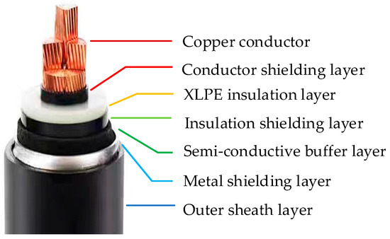
Figure 1.
The specific structure of single-core cables.
In Figure 1, a single-core power cable is mainly composed of an outer sheath layer, a metal shielding layer, a semi-conductive buffer layer, an insulation shielding layer, an XLPE insulation layer, a conductor shielding layer, and a copper conductor. Among them, the copper conductor is the conductive part of the cable, and its role is to transport electrical energy. The role of the XLPE insulation layer is to form electrical isolation between the core conductor and the outside world to ensure the safety of the cable. Due to manufacturing process issues, the insulation layer, the conductor, and the metal sheath will inevitably exist between the air gaps, burrs, and so on. The insulation shielding layer and the conductor shielding layer can eliminate the gaps between them while making the insulation layer inside and outside the surface, respectively, with the conductor and metal sheath equipotential to avoid partial discharge. The semi-conductive buffer layer can relieve the pressure of the outside world on the internal structure to avoid the damage caused by the metal sheath welding process on the insulating layer, but the metal sheath also plays a longitudinal role in blocking water. The metal shielding layer can shield the interference of the external electric field to form a ground zero potential. It also provides access to the short circuit fault current, to a certain extent, to protect the safe operation of the cable. The outer sheath layer commonly has polyethylene or PVC wrapped in the outermost surface of the cable to try to avoid external factors on the cable caused by mechanical damage and corrosion of certain chemical components, so that the cable can be laid in a variety of complex environments to ensure stable and good performance of power transmission. Due to the insulation shielding layer and conductor shielding layer being thin relative to the rest of the structure of the layer, in the calculation of the temperature field, ensuring calculation accuracy and reducing computational complexity can be attributed to the XLPE insulation layer.
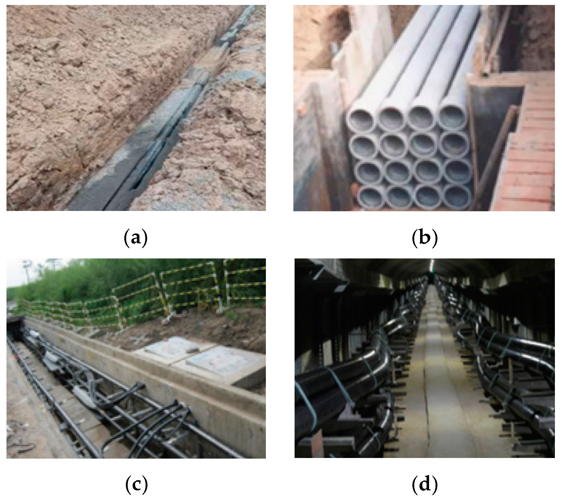
Cable laying methods generally include four ways: direct burial, pipe, cable trench, and tunnel. Figure 2 shows the diagram of different laying methods.

Figure 2.
Diagrams of different ways of laying cables: (a) Cable direct burial laying method; (b) Cable pipe laying method; (c) Cable trench laying method; (d) Cable tunnel laying method.
In Figure 2, direct burial laying is convenient and saves materials and labor. The construction cycle is short, but maintenance is inconvenient, and the cables are prone to mechanical damage and chemical or electrochemical corrosions due to the surrounding soil, as well as termites and rodent hazards, and troubleshooting requires digging up the road surface. Rows of pipe laying can be laid side by side when the numbers of cables increase and with the same path in the future. Carrying out the installation of cable routes, maintenance, or updating does not require repeated excavation of the road, but the civil engineering investment is larger. Cable trench laying is more convenient, the maintenance difficulty is lower, and an excavation after the construction of the cable can be successively casted according to the need to lay more to the cable. However, the construction cycle is longer, and the construction cost is higher. Tunnel laying greatly facilitates cable operation and maintenance for the cable operation and maintenance personnel to build a good operation and maintenance environment, but the cables occupy a larger space, the construction cycle is longer, and the construction cost is particularly high. Therefore, the actual cable laying can be based on the laying materials, labor input, construction cycle, and later operation and maintenance for a reasonable choice.
3. Power Cable Temperature Field and Current-Carrying Capacity Simulation and Calculation Modeling
When the power cables are buried directly in the ground, its heat is mainly transferred between the cable body and the soil by heat conduction, while for pipe laying and trench laying, due to the airflow between the inner wall of the casing and the cable, the three ways of heat convection, heat conduction, and heat radiation should be considered in the calculation of the amount of current-carrying capacity and the temperature field of the cable. Among them, the heat conduction control equation in the region with a heat source is shown in the following equation.
where qv is the volumetric heat generation rate in W/m3, and T is the medium temperature.
The heat transfer control equations for the region without heat source are shown below.
The natural convection of air in a discharge pipe or ditch can be described by the laws of mass conservation, momentum conservation, and energy conservation in a two-dimensional right-angle coordinate system, and the law of mass conservation is shown in Equation (3).
where u and v are components of velocity vector in the x-axis and y-axis flow fields, respectively, in m/s; ρ is the air density in kg/m3.
Neglecting the viscous dissipation of air and assuming that the physical parameters (except the air density) are constant, the momentum conservation equations in the air region are shown in Equations (4) and (5).
where η is the hydrodynamic viscosity in Pa·s, p is the pressure of the flow field in Pa, α is the coefficient of volumetric expansion in K−1, g is the gravitational acceleration in m/s2, Tr is the reference temperature of the fluid in K, and θ is the angle of gravitational acceleration with respect to the x-axis.
The energy equation of the air region is given in Equation (6), where the air layer is in a steady state, is a single substance, and does not account for viscous dissipation, radiation, and internal heat sources.
where λ is the material coefficient of thermal conductivity and is able to reflect the thermal conductivity of the material, which is an important parameter. The size of the value will be affected by the temperature and other factors, generally determined through relevant tests, and its unit is W/(m·K).
For drain laying and trench laying, there is also heat radiation from the inside of the drain or trench and the cable surface, which can be expressed as Equation (7).
where Qi is the heat transfer of area cell i, εi is the thermal emissivity of area cell i, δ is the Stefan–Boltzmann constant, Fij is the angular coefficient of area cells i and j, Ai is the area of area cell i, and Ti and Tj are the absolute temperature values of area cells i and j, respectively.
In the setting of boundary conditions, known boundary normal heat flux, known boundary temperature, and convection boundary conditions are three types of boundary conditions. The governing equations are shown below.
where q2 is the heat flow density in W/m2, k is the thermal conductivity in W/(m·K), Tf is the fluid temperature in K, h is the convective heat transfer coefficient in W/(m2·K), and Γ is the integration boundary.
In this test, the boundary conditions under the three laying methods are set in the same way; the soil exchanged heat with the air in the form of convection, and the convective heat transfer coefficient is taken to be 12.5 W/(m2·K). The deeper soil is set as a known boundary temperature, i.e., the temperature is a constant value, taken to be 8 °C, and the soil on the right side and the soil on the left side are set as a known boundary normal to the density of heat flow, i.e., the density of the heat flow along the normal direction is zero.
Using the double-point chordal intercept method to calculate the current-carrying capacity of cables, i.e., first select two different currents, I1 and I2, and calculate the maximum temperatures T1 and T2 corresponding to the cables, respectively, on the basis of calculating the current-carrying capacity using the double-point chordal intercept method, and its solution formula is shown below.
where Ik+1, Ik, and Ik−1 are the cables’ carrying capacities calculated for k + 1-th, k-th, and k−1-th, and f(Ik) and f(Ik−1) are the cables’ maximum temperatures calculated according to Ik and Ik−1, respectively.
Since the XLPE cable is allowed to work at a maximum temperature of 90 °C for a long time, the conditions constrained by the algorithm for calculating the cable’s carrying capacity is shown below.
where ε is the set threshold. In order to take into account the requirements of algorithm accuracy and solution speed, through many experiments, the threshold is taken as 0.1 °C in the paper.
The double-point chordal interception method is used to calculate the carrying capacity of the cable. The steps are shown below.
- Step 1: Randomly select the current value as Ik−1 and calculate f(Ik−1) at this point. If the target is satisfied, then Ik−1 is the required carrying capacity; otherwise, go to Step 2.
- Step 2: Randomly select the current value as Ik and calculate f(Ik) at this point. If it meets the requirements, then Ik is the required amount of current-carrying capacity; otherwise, go to Step 3.
- Step 3: Calculate the value of the carrying capacity Ik+1 according to Equation (11) and calculate f(Ik+1). If it meets the requirements, then Ik+1 is the required carrying capacity; otherwise, go to Step 4.
- Step 4: Let Ik−1 = Ik, f(Ik−1) = f(Ik), Ik = Ik+1, and f(Ik) = f(Ik+1); go to Step 3.
4. Calculation Results and Analysis
In order to analyze the current-carrying capacity and temperature field changes of cables in different laying modes, the XLPE cables with cable type 64/110 kV-YJLW-02-630 mm2 are taken as the object of study, and the temperature field of cables is simulated and calculated using COMSOL Multiphysics. The geometric dimensions of each part of the structure of the power cable are given in Table 1; the laying conditions of power cables and the physical parameters of the material are given in Table 2.

Table 1.
Geometric dimensions of the structure of the parts of the power cable.
Table 2.
Power cable laying conditions and material physical parameters.
The existing research shows that the impact of cable heat at a distance of 2 m away from the outside of the is weak and does not affect heat transfer around the cable, which should be set when the regional scope is large enough. When 20 m away from the cable, the temperature of the soil is no longer influenced by cable heat. Now, to ensure the accuracy of model calculations, a distance from the cable of below 20 m for the soil depth is selected, so that the boundary is far enough from the cable, the temperature is constant, and this belongs to the first category of boundary conditions. From the cable, around 20 m for the right and left boundaries of soil, the boundary is far enough from the cable, and the density of heat flow does not change, which belongs to the second category of boundary conditions. The existence of convection air and the upper boundary of the soil heat transfer belong to the third boundary condition.
4.1. Simulation Analysis of Temperature Field and Current-Carrying Capacity of Cable under the Direct Burial Laying Method
In the power cable direct burial laying model, cable conductor spacing is set at 250 mm, and the cable laying depth is 1 m. Through finite element simulations, when the temperature of the cable conductor is the highest at 90 °C, the cable current-carrying capacity is calculated to be 938 A. The other two phases of the cable had maximum temperatures of 85.80 °C and 86.18 °C, respectively. The temperature field distribution of the power cable is illustrated in Figure 3; the maximum temperature occurs in the middle cable conductor, and the lowest temperature occurs in the lower boundary of the soil, which is 8 °C.
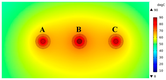
Figure 3.
Temperature field distribution of cables under the direct burial laying method.
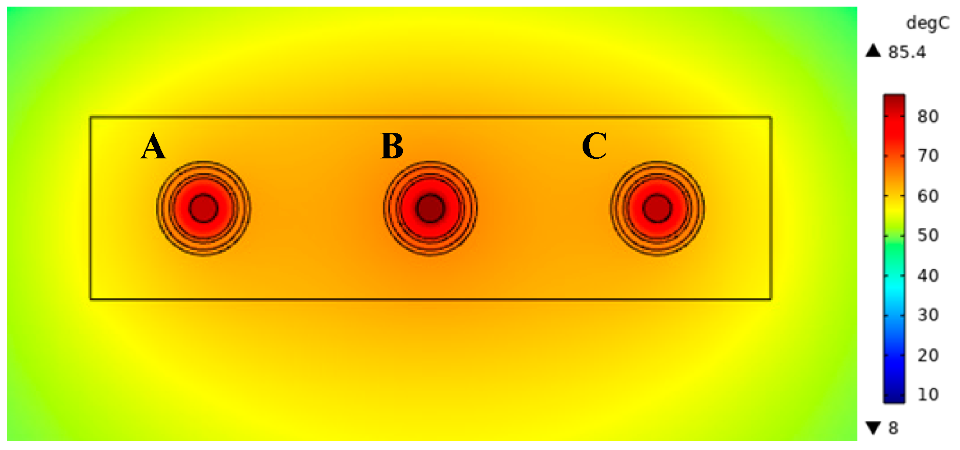
According to the power engineering cable design standards, the cable will be laid directly buried around a layer of sand backfill to avoid soil moisture migration on flow-carrying caused by a greater impact. Studying the backfill sand and backfill type of direct burial cable laying on the impact of flow, moist sand and dry sand thermal conductivity show 2 W/(m·K) (15% moisture content) and 1.5 W/(m·K) (9% moisture content) along the cable axis and up and down the immediate sides of 100 mm sand thickness. Without changing the other laying conditions, backfill moist sand laying is still applied to the cable conductor with the same carrier flow of 938 A. The three-phase cable conductor temperature field distribution is illustrated in Figure 4.

Figure 4.
Temperature field distribution of cables laid on backfilled moist sandy soil.
From Figure 4, the temperature of the B-phase cable is the highest at 85.44 °C, and the highest temperature of the A-phase and C-phase cables are 82.34 °C and 82.63 °C, respectively, when backfilled moist sandy soil is laid. Similarly, without changing other laying conditions, the three-phase cable conductor in dry sandy soil under the carrying capacity of 938 A is obtained, the cable’s carrying capacity is calculated by the double-point chordal interception method, and the temperatures and carrying capacities of the three-phase cable conductors under different backfilled sandy soil types are obtained, as shown in Table 3.
Table 3.
Temperature and carrying capacity of three-phase cable conductor when backfilling sand.
From Table 3, compared with backfilling with virgin soil, when backfilling with dry sandy soil and moist sandy soil, the conductor temperature of three-phase cables is reduced, and the highest decreases in conductor temperature are about 2.98 °C and 4.56 °C, and cables’ carrying capacities are improved by 1.92% and 3.09%, respectively. Direct burial laying is mainly heaty conduction between solids, where the heat generated by cables is transferred to the surrounding environment through soil/sand thermal conductivity. The backfill of sand is more conducive to cable heat dissipation. The thermal conductivity of the moist sand is stronger than that of the dry sand, and the heat dissipation capacity is stronger, so the three-phase cable conductor temperatures are relatively low, showing maximum flow-carrying capacity. In addition, by increasing the thickness of sand and sand moisture content, the cable’s carrying capacity can also be enhanced to different degrees.
4.2. Simulation Analysis of Cable Temperature Field and Current-Carrying Capacity under the Discharge Pipe Laying Method
Power cable pipe laying needs to be pre-buried in the ground cement or plastic pipe, and then the power cable through the pipe laying. Due to China Southern Power Grid Company’s laying pipes generally having 3 × 4 specifications, these specifications of the pipe will also be used in this paper. Simulation selection of PVC pipe includes an inner radius of 125 mm, outer radius of 135 mm, and wall thickness of 10 mm. For the pre-laying of the pipe, the distance between the axes of the pipe is 300 mm, the pipe is buried 1 m deep underground, and the lowest layer of the pipe is 20 m away from deep soil, with the left and right sides of the pipe being 20 m away from left and right borders. When setting the material parameters, the inner part of the pipe is ordinary air; the pipe is made of PVC material, and its thermal conductivity is 0.1667 W/(m·K). The material parameters of the cable and soil are the same as those mentioned before, and the boundary condition setting is the same as that of the previous calculation case.
For single-circuit cable duct laying up and down a zigzag arrangement structure, through the finite element simulation, when the cable temperature is maximum at 90 °C, cable current-carrying capacity is calculated to be 855 A. The maximum temperature of the B-phase cable is 90 °C, while the maximum temperatures of A-phase and C-phase cables are 86.78 °C and 82.85 °C, respectively. The temperature field distribution of the power cable is illustrated in Figure 5.
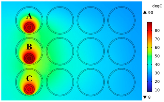
Figure 5.
Temperature field distribution of single-circuit cable duct laying with the upper and lower zigzag arrangement.
In Figure 5, the highest temperature occurs above cable B because the power cable in the middle phase is more affected by the heat generated by other phase cables, and the middle position is not conducive to the conduction of heat into soil. When power cables are laid in the row of pipes, the heat loss is first conducted through air convection, then through the PVC row of pipes, and finally, by the soil to conduct heat. Due to the small space inside the row of pipes, the air is not able to flow sufficiently to conduct heat, so the air temperature inside the tube is higher; therefore, compared with the direct burial method of laying, the power cable’s current-carrying capacity in the way of the row of pipe laying is smaller.
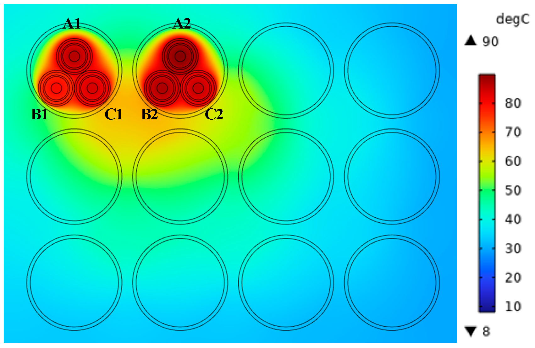
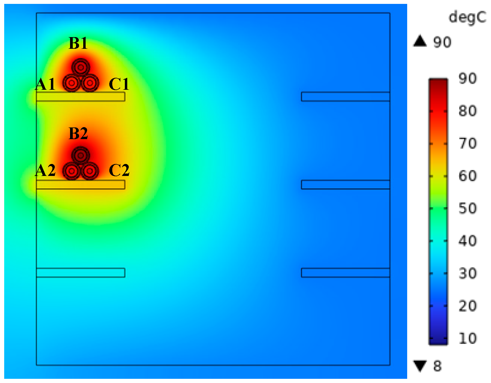
In this section, the current-carrying capacity and temperature field of double-circuit power cables laid in PVC plastic pipes are calculated and analyzed in different arrangements. Double-circuit power cables include three types of arrangements: upper and lower zigzag arrangement, horizontal triangular arrangement, and upper and lower triangular arrangement. For the upper and lower zigzag arrangement model, when the temperature of the cable conductor is 90 °C, the calculated cable current-carrying capacity is 719 A; at this time, the double-circuit cable pipe laying up and down the zigzag arrangement of the temperature field distribution is illustrated in Figure 6.
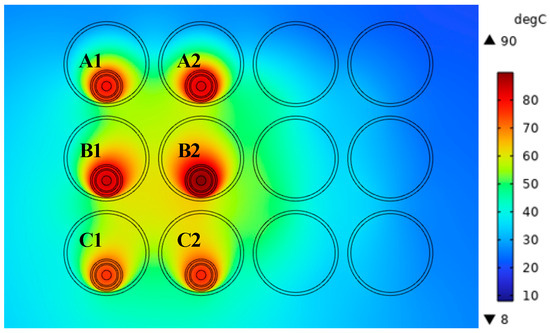
Figure 6.
Temperature field distribution of double-circuit cable duct laying with the upper and lower zigzag arrangement.
Duct-laying double-circuit power cables arranged in a zigzag pattern above and below each cable conductor temperature are shown in Table 4.
Table 4.
Double-circuit cable duct laying up and down a zigzag arrangement of each cable conductor temperature.
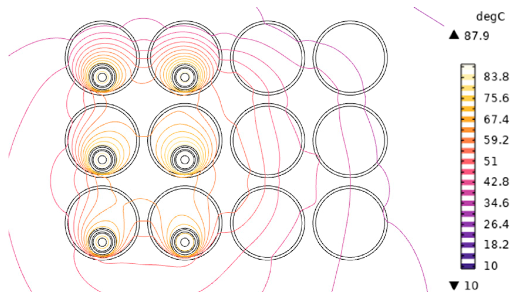
In Figure 6, for the duct where the highest temperature of B2 cable is located, the air temperature inside the discharge pipe is between about 58 and 84 °C. The PVC discharge pipe has poor heat dissipation performance, and its internal temperature is also between 57 and 64 °C. When the power cable is laid in the tube, the heat loss first passes through the air convection, then conducts heat through the PVC tube, and finally, the soil conducts heat. Because the space inside the tube is small, the air cannot flow sufficiently to conduct heat, making the air inside the tube high in temperature. The power cable of the intermediate phase is greatly affected by the heating of other phase cables, and the middle position is not conducive to the conduction of heat to the soil, so the temperature of the B1 and B2 phases is higher, while the C1 phase is located deep in the soil and has a large contact area with the soil, which is more conducive to the conduction of heat, so the C1-phase cable has the lowest temperature. The isotherm distribution obtained from Figure 6 is shown in Figure 7.
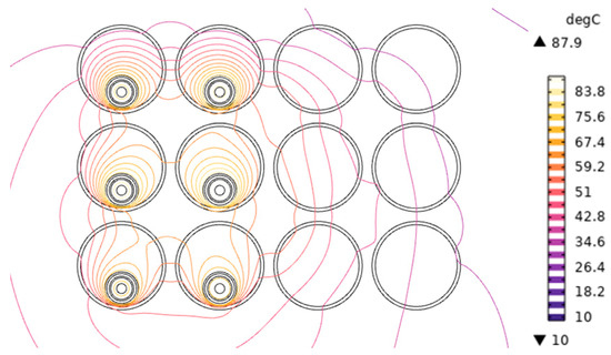
Figure 7.
Isothermal distribution diagram of double-circuit cable duct laying up and down in a zigzag arrangement.
From Figure 7, the isotherms in the area far from the power cable are distributed sparsely, while the isotherms in the area near the power cable are distributed very densely.
When power cables are arranged in a horizontal triangle way inside the row of pipes, generally, three power cables are laid in a pipe, and the relevant geometric parameters, physical parameters, and boundary condition settings are the same as the previous settings. In this case, the two outermost rows of pipes are selected for laying because the outermost rows of pipes have good heat dissipation conditions and are more conducive to the design of power cable capacity increase. When the temperature of the cable conductor is up to 90 °C, the cable’s current-carrying capacity is 655 A; at this time, the double-circuit power cable pipe laying horizontal triangular arrangement of the temperature field distribution is as shown in Figure 8.

Figure 8.
Temperature field distribution of the horizontal triangular arrangement of double-circuit cable duct laying.
The temperature of each cable conductor for a horizontal triangular arrangement of double-circuit power cable duct laying is shown in Table 5.
Table 5.
Double-circuit cable duct laying horizontal triangular arrangement of each cable conductor temperature.
In Figure 8, the pipeline where the A2 cable is located has the highest temperature, which makes the temperature above the row of pipes higher due to the upward flow of heated air. Due to a row of pipes laying three power cables, the space occupation is relatively large and the airflow space is small and is not conducive to fluid heat conduction. For the row of pipes closely installed to three power cables, the interactions between the cables are large, so the current-carrying capacity is very small in this way of laying.
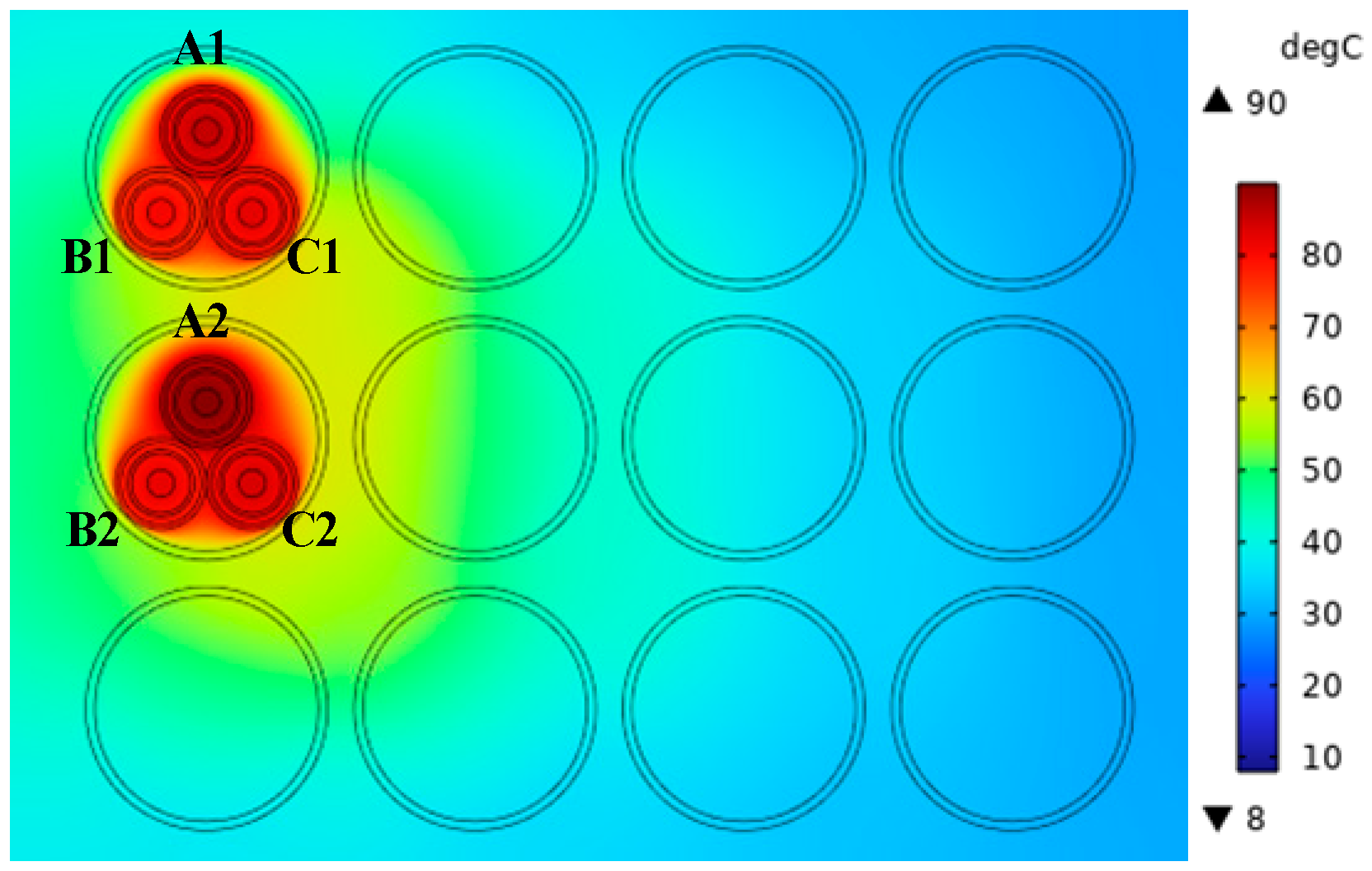
For power cables arranged in the lower and upper triangular way inside the tube, when the temperature of the cable conductor is up to 90 °C, the calculated cable current-carrying capacity is 657 A; at this time, the double-circuit cable tube laying up and down the triangular arrangement of the temperature field distribution is as shown in Figure 9.

Figure 9.
Temperature field distribution of the upper and lower triangular arrangement of double-circuit cable duct laying.
Double-circuit cable duct laying up and down in a triangular arrangement of each cable conductor temperature is shown in Table 6.
Table 6.
Double-circuit cable duct laying up and down in a triangular arrangement of each cable conductor temperature.
In Figure 9, the pipeline where the A2 cable is located has the highest temperature, affected by the depth of the soil; the upper and lower triangular arrangement of heat dissipation is better than the horizontal triangular arrangement, so compared with the horizontal triangular arrangement of the double-circuit power cable row pipe laying, the upper and lower triangular arrangement of the structure of the flow-carrying capacity is increased by 2 A.
4.3. Simulation Analysis of Cable Temperature Field and Current-Carrying Capacity under the Trench Laying Method
Due to cable trench laying and tunnel laying having the same space structure, the cable temperature field and the change rule of carrier flow are the same, so the trench laying method is used as an example for research. Trench laying is a very important mode of laying cables; the trench is full of air, so the cable trench part of the thermal conductivity problem belongs to the fluid heat conduction, and the trench outside the soil shows solid heat conduction. This kind of laying is more widely used in urban construction. The size of the cable trench is selected as 2 m × 2 m, the spacing of the bracket is 500 mm, the distance between the trench wall and the right and left boundaries of the soil is 20 m, the distance between the bottom of the trench and the boundary of the deep soil is 20 m, and the trench is near the ground as a cover. A certain width is reserved for the representation in the model, and the other relevant geometrical parameters, physical parameters, and boundary condition settings are the same as the previous settings.
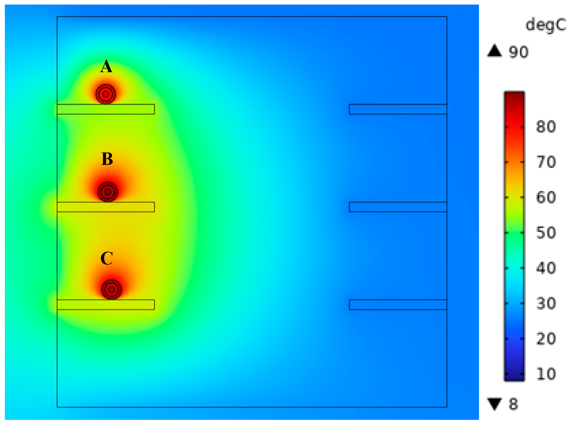
When single-circuit cable trench laying up and down a zigzag arrangement, through the finite element simulation, the temperature of the cable conductor is maximum at 90 °C, and the calculated cable current-carrying capacity is 892 A, in which the maximum temperature of the B-phase cable is 90 °C, and the maximum temperatures of the A-phase and C-phase cables are 83.72 °C and 88.06 °C, respectively. The distribution of the temperature field of the power cable is illustrated in Figure 10.
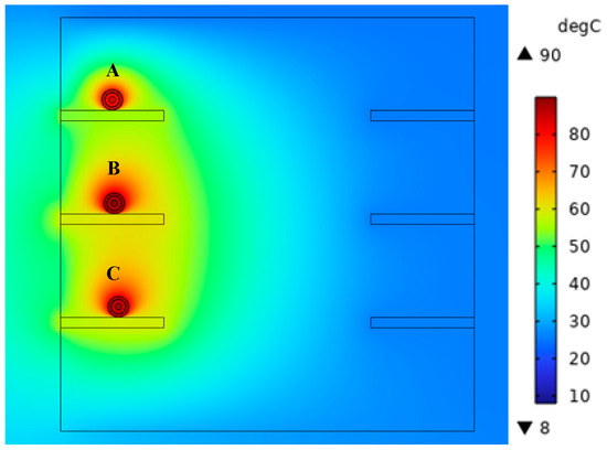
Figure 10.
Temperature field distribution of single-circuit cable trench laying with the upper and lower zigzag arrangement.
When single-circuit cable trench laying up and down a zigzag arrangement, the highest temperature appears in the B-phase cable, while the A-phase cable temperature is the lowest. This is due to the existence of airflow inside the cable trench; the trench above the internal distance from the ground is only spaced by a trench cover. When air flows faster, the cable body can be emitted by the heat away from a part of the body, so the A-phase cable temperature is the lowest, while the B-phase cables are in the center, by the A-phase and C-phase cables and airflow, so the temperature is the highest.
When the single-circuit cable trench laying is arranged horizontally through the finite element simulation, the temperature of the cable conductor is up to 90 °C, and the cable current-carrying capacity is calculated to be 759 A, in which the highest temperature of the C-phase cable is 90 °C, while the highest temperatures of the A-phase and B-phase cables are 85.76 °C and 89.98 °C, respectively. The distribution of the temperature field of the power cable is illustrated in Figure 11; due to convection of air, both the B-phase and C-phase cables show high temperatures close to 90 °C.
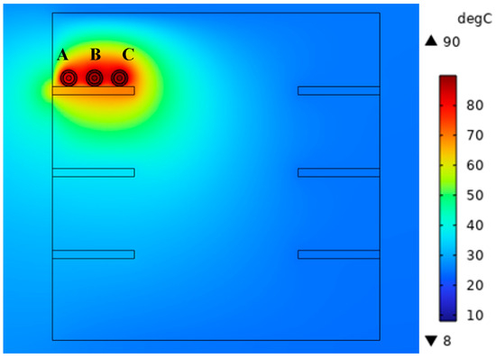
Figure 11.
Temperature field distribution of single-circuit cable trench laying in the horizontal arrangement.
When single-circuit cable trench laying in a triangular arrangement, through the finite element simulation calculation, the temperature of the cable conductor is the highest at 90 °C, and the current-carrying capacity of the cable is calculated to be 672 A, in which the highest temperature of the B-phase cable is 90 °C, while the highest temperatures of the A-phase and C-phase cables are 81.83 °C and 82.20 °C. The distribution of the temperature field of the power cable is shown in Figure 12; the triangular arrangement of the cable between the phases of heat transfer and cable arrangement congestion are not easy for airflow, so the cable’s carrying capacity is smaller.
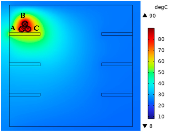
Figure 12.
Temperature field distribution of single-circuit cable trench laying in a triangular arrangement.
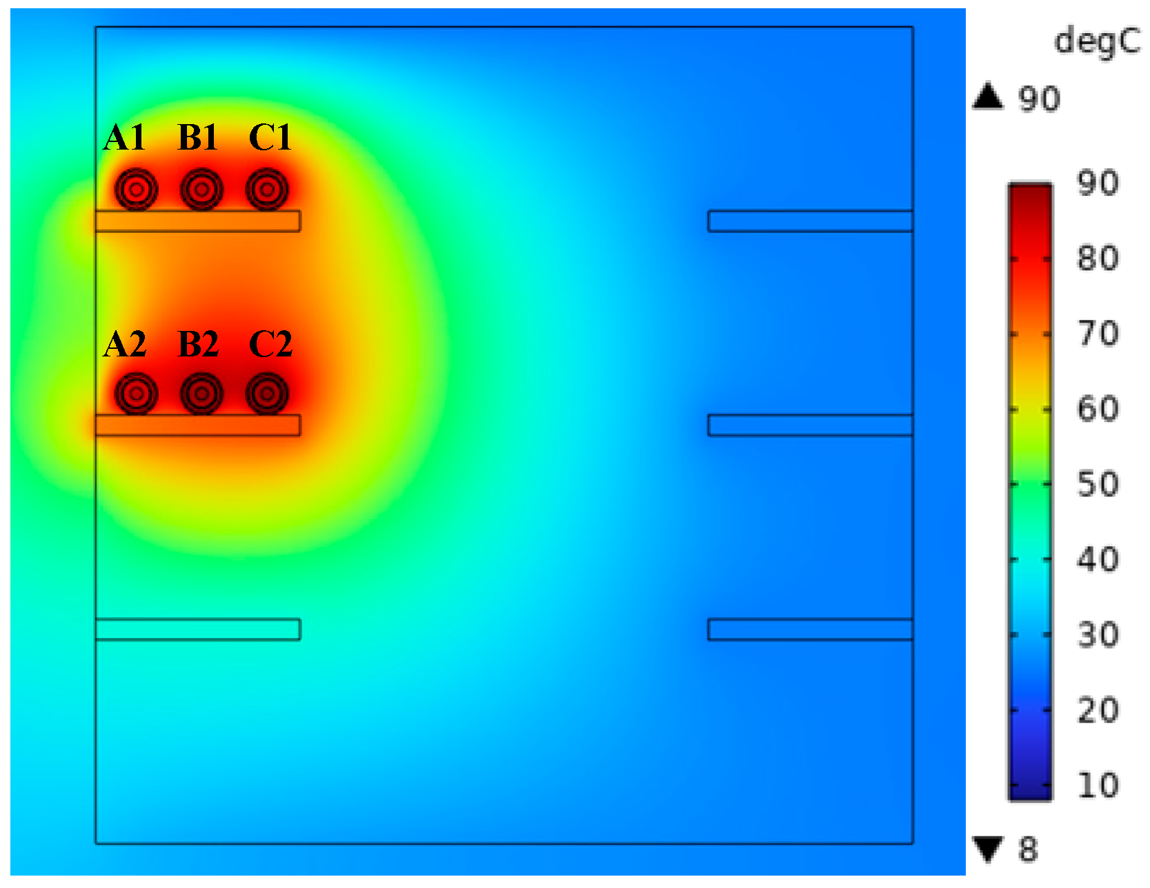
When double-circuit cable trench laying up and down in a horizontal arrangement, through finite element simulation calculations, the temperature of the cable conductor is the highest at 90 °C, and the cable’s current-carrying capacity is calculated to be 671 A, in which the highest temperature of the C2-phase cable is 90.04 °C. The temperature field distribution of the power cable is illustrated in Figure 13.
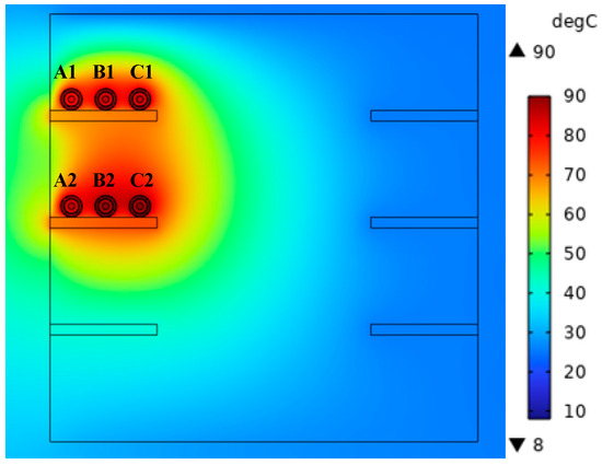
Figure 13.
Temperature field distribution of double-circuit cable trench laying with up and down horizontal alignment.
Double-circuit cable trench laying with up and down horizontal arrangement of each cable conductor temperature is illustrated in Table 7.
Table 7.
Double-circuit cable trench laying with up and down horizontal arrangement of each cable conductor temperature.
When double-circuit power cables are laid horizontally up and down in the trench, the cable heat generation affects each other, but because the cable is surrounded by flowing air, air convection causes faster heat transfer, making this thermal interaction not very obvious, so the conductor temperature difference between different cables is not very big, but under the action of the airflow field, the cable near the aisle has a higher temperature.
When double-circuit cable trench laying with an upper and lower triangular arrangement, through the finite element simulation calculation, the temperature of the cable conductor is the highest at 90 °C, and the calculated cable current-carrying capacity is 608 A, of which the highest temperature of the B2-phase cable is 90.05 °C. The temperature field distribution of the power cable is shown in Figure 14.

Figure 14.
Temperature field distribution with upper and lower triangular arrangement of double-circuit cable trench laying.
Double-circuit cable trench laying with up and down triangular arrangement of each cable conductor temperature is shown in Table 8.
Table 8.
Double-circuit cable trench laying with up and down triangular arrangement of each cable conductor temperature.
In Figure 14, the temperature of the power cables with triangular arrangement is higher because the air is heated in an upward flow; before the lower temperature of the air squeezed out, it is squeezed out of the cold air to the other parts of the flow back to where the cable is heated, and then it rises again, until a dynamic equilibrium is reached, so the B-phase cable temperature is higher than those of the A-phase and C-phase. The B1-phase cables from the ground are only spaced by a trench cover, so air flows faster, and the heat emitted by the cable body can be taken away since part of the B1-phase cable temperature is lower than the B2-phase cable temperature.
4.4. Analysis of Temperature Field and Current-Carrying Capacity Calculation Results under Different Laying Methods of Power Cables
In this paper, the current-carrying capacity and temperature field of power cables in different arrangements under three laying modes of power cables—directly buried, rows of pipes, and trenches—are simulated and analyzed in detail, and the current-carrying capacity under different laying methods is shown in Table 9.
Table 9.
Carrying capacity of power cables under different laying methods.
As can be seen from Table 9, the more centralized the distribution of cables, the lower the current-carrying capacity, and backfilling with a certain amount of sand can improve the current-carrying capacity when the cables are laid. For a single-circuit power cable arrangement, due to the triangular arrangement of power cables with a small distance between each other, the heat dissipation space is not as good as the upper and lower zigzag arrangement or the horizontal arrangement of power cables, so the triangular arrangement of power cables will have a smaller current-carrying capacity. From the size of the flow-carrying point of view, the direct burial laying method of cable flow-carrying is the largest, followed by pipe laying, while trench laying is the smallest. However, the direct burial laying method is inconvenient to maintain, easy to be damaged by mechanical external forces and the chemical or electrochemical corrosion from the surrounding soil, as well as termites and rodent hazards, and troubleshooting requires digging up the roadway and the inputs of pipe laying and trench laying, which will greatly increase the construction costs. In addition, this paper mainly carries out the simulation calculations of current-carrying capacity and temperature field for single-circuit and double-circuit laying methods, and further in-depth research can be carried out on multi-circuit laying methods, different laying depths, different laying spacings, and different load intensities. In the simulation experiment, the current flow through which the cable can withstand the maximum temperature when transporting electric energy is set to the current-carrying capacity. Since the maximum temperature of the cable is set to 90 °C each time, and the cable spacing is set to be small, the temperature change of different phases of the cable is very small, but the download flow will vary greatly in different laying methods.
5. Conclusions
This paper focuses on XLPE cables, simulates and analyzes the current-carrying capacity and temperature field of single-circuit and double-circuit power cables in different arrangements under three laying modes—directly buried, row pipe, and trench—and builds a theoretical model for the calculation of the current-carrying capacity and temperature field of power cable with three thermal conductivity modes, including heat convection, heat conduction, and heat radiation. It also puts forward a method of calculating cable current-carrying capacity based on the double-point chordal intersection method. By using COMSOL software, the simulation model conforming to the actual cable laying method is established. Through the simulation results and analyses, the cable laying method greatly affects cable capacity; the directly buried laying method’s cable load capacity is the largest, followed by pipe laying, while trench laying is the smallest, and the more centralized the distribution of cables, the smaller the load capacity; the more decentralized the distribution, the greater the load capacity. Backfilling with a certain amount of sand can improve the load capacity in a closed cable trench. At the same time, in an enclosed cable, after the temperature reaches a steady state, the air in the ditch velocity is slow, so convection ventilation equipment needs to be added to improve the carrying capacity of the cable. The simulation calculation method proposed can calculate the load capacity of power cables under different laying modes in real time, quantify power cables’ current-carrying capacities, and reduce the risk of thermal aging of the cable insulation layer, which is of great significance to ensure the safe and economic operation of cables.
Author Contributions
Conceptualization, Y.N. and D.C.; methodology, S.Z.; software, S.Z.; validation, Y.N., X.X., and Z.W.; formal analysis, S.Z.; investigation, X.W.; resources, X.X.; data curation, Z.W.; writing—original draft preparation, S.Z.; writing—review and editing, Z.W.; visualization, Y.N.; supervision, D.C.; project administration, X.W.; funding acquisition, Z.W. All authors have read and agreed to the published version of the manuscript.
Funding
The authors declare that this study received funding from the China Southern Power Grid Company Limited’s Science and Technology Projects (YN-KJXM20240027). The funder was not involved in the study design, collection, analysis, interpretation of data, the writing of this article or the decision to submit it for publication.
Data Availability Statement
The original contributions presented in the study are included in the article, further inquiries can be directed to the corresponding author.
Conflicts of Interest
Authors Yongjie Nie, Daoyuan Chen, Xiaowei Xu were employed by the Electric Power Research Institute, Yunnan Power Grid Co., Ltd. The remaining authors declare that the research was conducted in the absence of any commercial or financial relationships that could be construed as a potential conflict of interest.
References
- Zhang, H.; Yu, S.; Liu, Z.; Cheng, X.; Zeng, Y.; Shu, J.; Liu, G. Research on the improvement of cable ampacity in dense cable trench. Energies 2024, 17, 2579. [Google Scholar] [CrossRef]
- Chang, S.J.; Kwon, G.Y. Anomaly detection for shielded cable including cable joint using a deep learning approach. IEEE Trans. Instrum. Meas. 2023, 72, 3516410. [Google Scholar] [CrossRef]
- Brakelmann, H.; Anders, G.J. Ampacity calculations of underground power cables with end effects. IEEE Trans. Power Deliv. 2023, 38, 1968–1976. [Google Scholar] [CrossRef]
- Meng, F.; Chen, X.; Hong, Z.; Shi, Y.; Zhu, H.; Muhammad, A.; Paramane, A.; Huang, R.; Han, Z. Insulation properties and interfacial quantum chemical analysis of cross-linked polyethylene under different degassing time for HVDC cable factory joint applications. IEEE Trans. Dielectr. Electr. Insul. 2023, 30, 271–278. [Google Scholar] [CrossRef]
- Vyatkin, V.S.; Kiuchi, M.; Otabe, E.S.; Ohya, M.; Matsushita, T. Enhanced current-carrying capacity of three-layer cable composed of Bi-2223 tapes using the longitudinal field effect. IEEE Trans. Appl. Supercond. 2015, 25, 5400404. [Google Scholar] [CrossRef]
- Mohamed, A.Z.E.D.; Zaini, H.G.; Gouda, O.E.; Ghoneim, S.S.M. Mitigation of magnetic flux density of underground power cable and its conductor temperature based on FEM. IEEE Access 2021, 9, 146592–146602. [Google Scholar] [CrossRef]
- Zhang, Y.; Yu, F.; Ma, Z.; Li, J.; Qian, J.; Liang, X.; Zhang, J.; Zhang, M. Conductor temperature monitoring of high-voltage cables based on electromagnetic-thermal coupling temperature analysis. Energies 2022, 15, 525. [Google Scholar] [CrossRef]
- Ei-kady, M.A.; Anders, G.A.; Motlis, J.; Horrocks, D.J. Modified values for geometric factor of external thermal resistance of cables in duct banks. IEEE Trans. Power Deliv. 1988, 3, 1303–1309. [Google Scholar] [CrossRef]
- Wu, J.; Chen, L.; Yan, Y.; Zhao, P. Study on temperature distribution of ±500 kV HVDC XLPE cable and its influencing factors. High Volt. Appar. 2023, 59, 113–119. [Google Scholar]
- Ma, A.; Zhang, Y. Thermal circuit model of EHV cable laid in tunnel considering mutual thermal effect. High Volt. Eng. 2022, 48, 1068–1076. [Google Scholar]
- Le, Y.; Zheng, X.; Zhang, Z.; Li, S.; Chen, G.; Zhang, L.; Lu, Z. Numerical caculation of ampacity for multi-loop cable system in ducts based on electromagnetic-thermal-flow coupled field. Sci. Technol. Eng. 2017, 17, 197–202+261. [Google Scholar]
- Wang, Y.; Chen, R.; Chen, W.; Yuan, Y. Calculation of trench laying cable ampacity and its influencing factors. Electr. Power Autom. Equip. 2010, 30, 24–29. [Google Scholar]
- Ozyesil, O.; Altun, B.; Demirol, Y.B.; Alboyaci, B. The effect of the vertical layout on underground cable current carrying capacity. Energies 2024, 17, 674. [Google Scholar] [CrossRef]
- Xu, X.; Yuan, Q.; Sun, X.; Hu, D.; Wang, J. Simulation analysis of carrying capacity of tunnel cable in different laying ways. Int. J. Heat Mass Transf. 2019, 130, 455–459. [Google Scholar] [CrossRef]
- Hu, Z.; Ye, X.; Li, Q.; Luo, X.; Zhao, Y.; Zhang, H.; Zhang, L. Analysis on three-core power cable temperature field and ampacity model under typical laying environment. Front. Energy Res. 2024, 12, 1430501. [Google Scholar] [CrossRef]
- Che, C.; Yan, B.; Fu, C.; Li, G.; Qin, C.; Liu, L. Improvement of cable current carrying capacity using COMSOL software. Energy Rep. 2022, 8, 931–942. [Google Scholar] [CrossRef]
- Qiao, J.; Zhao, X.; Xia, Y.; Feng, Y.; Xiao, Y.; Yang, L. Simulation analysis of steady-state ampacity of ±500 kV high-voltage DC submarine cables under different laying methods. High Volt. Eng. 2023, 49, 597–607. [Google Scholar]
- Chen, X.; Wang, Q.; Yu, J.; Yao, G. Simulation research on DC ampacity of 10 kV AC XLPE cable under different DC operation topologies and laying modes. High Volt. Eng. 2021, 47, 4044–4054. [Google Scholar]
- Chippendale, R.D.; Pilgrim, J.A.; Goddard, K.F.; Cangy, P. Analytical thermal rating method for cables installed in j-tubes. IEEE Trans. Power Deliv. 2017, 32, 1721–1729. [Google Scholar] [CrossRef]
- Gouda, O.E.; Dein, A.Z.E.; Amer, G.M. Effect of the formation of the dry zone around underground power cables on their ratings. IEEE Trans. Power Deliv. 2011, 26, 972–978. [Google Scholar] [CrossRef]
- Chatzipetros, D.; Pilgrim, J.A. Impact of proximity effects on sheath losses in trefoil cable arrangements. IEEE Trans. Power Deliv. 2020, 35, 455–463. [Google Scholar] [CrossRef]
- Sedaghat, A.; Lu, H.; Bokhari, A.; Leon, F.D. Enhanced thermal model of power cables installed in ducts for ampacity calculations. IEEE Trans. Power Deliv. 2018, 33, 2404–2411. [Google Scholar] [CrossRef]
- Hanna, M.A.; Chikhani, A.Y.; Salama, M.M.A. Thermal analysis of power cables in multi-layered soil part I: Theoretical model. IEEE Trans. Power Deliv. 1993, 8, 761–771. [Google Scholar] [CrossRef]
- Zhang, H.; Yin, Y.; Xie, S.; Hu, M.; Fan, Y.; Li, X. Calculation and testing research on current rating capacity of XLPE insulated HVDC cable with different metallic screen type. High Volt. Eng. 2021, 47, 2117–2123. [Google Scholar]
- Liang, Y.; Yan, C.; Zhao, J.; Sun, K.; Liu, J. Numerical calculation of transient temperature field and sort-term ampacity of group of cables in ducts. High Volt. Eng. 2011, 37, 1002–1007. [Google Scholar]
- Yang, Y.; Cheng, P.; Chen, J.; Yang, F. Current-carrying capacity calculation based on coupling fields for cable in ventilated trench and its influencing factors. Electr. Power Autom. Equip. 2023, 33, 139–143+154. [Google Scholar]
- Bian, X.; Chen, Y.; Zhou, Q.; Zhang, Y.; Wei, B.; Tong, P. Dynamic temperature field calculation and short-time allowable ampacity evaluation of submarine cable based on thermal analytical model. High Volt. Eng. 2023, 49, 793–802. [Google Scholar]
- Wang, Q.; Wang, G.; Yu, J.; Chen, X. Research on simulation of DC current-carrying capacity of clustered cables laying under various laying modes. High Volt. Appar. 2022, 58, 157–164. [Google Scholar]


Disclaimer/Publisher’s Note: The statements, opinions and data contained in all publications are solely those of the individual author(s) and contributor(s) and not of MDPI and/or the editor(s). MDPI and/or the editor(s) disclaim responsibility for any injury to people or property resulting from any ideas, methods, instructions or products referred to in the content. |
© 2024 by the authors. Licensee MDPI, Basel, Switzerland. This article is an open access article distributed under the terms and conditions of the Creative Commons Attribution (CC BY) license (https://creativecommons.org/licenses/by/4.0/).