Abstract
This paper presents a model-based PID tuning method for a reactor used in microwave-assisted chemistry. The reactor is equipped with a solid-state source of microwaves and a PID controller capable of increasing or decreasing the delivered microwave power to maintain the reacting substances at the desired temperature. The model has the form of an algorithm applied in numerical simulations of two simultaneous processes: heating a substance by absorbing microwave radiation and cooling it by dissipating heat to the surroundings. It has proven its suitability for tuning the PID controller in a time-efficient manner. Despite some noticeable inaccuracies, the presented approach easily finds PID coefficients that result in stable and repeatable controller operation. In this way, significant time savings can be achieved, as well as minimizing the risks associated with, for example, boiling liquid spills. The article demonstrates that a carefully designed, but still relatively simple, model can yield significant benefits in tuning PID controllers.
1. Introduction
Microwaves occupy a part of the electromagnetic spectrum between 300 MHz and 300 GHz, corresponding to a wavelength ranging from 1 m to 1 mm. Their ability to heat various kinds of materials was discovered decades ago, and it is currently widely used in many fields of science and industry [1,2,3,4].
In chemistry, it has been observed that certain reactions assisted by microwave irradiation resulted in enhancing reaction rates, selectivity, and yields compared with conventional heating [5,6]. For this reason, much attention is being paid to microwave reactors—devices that allow the reaction mixture to be exposed to a microwave field.
Typically, a microwave reactor consists of a high-power microwave source coupled to a cavity comprising a reaction vessel. In continuous flow designs, the reaction vessel allows the mixture to flow through the cavity at the desired flow rate. In batch reactors, the vessel contains a fixed volume of reagents, optionally mixed to prevent unwanted sedimentation and equalize the temperature [7,8].
In the case of conventional heating, heat is first supplied to the walls of the vessel and only then dissipated into its contents. In contrast, microwaves penetrate the vessel and transfer their energy directly to the molecules of the reacting compounds, providing more or less volumetric heating, which provides a number of benefits. The desired temperature is reached faster, and the reaction time decreases. Accordingly, the formation risk of side products also decreases, and the final product purity increases [9]. Unwanted temperature gradients and local overheating in the volume of the mixture can be avoided. Overheating (superheating) is an undesirable effect during a chemical reaction due to the possibility of sintering or melting certain compounds, causing their degradation. The microwave power can be precisely controlled, which, in consequence, allows one to control the temperature over time. This, in turn, provides reproducible reaction conditions.
In addition to the above thermal effects, numerous researchers have reported that the mere presence of a microwave field can affect the rate and results of a chemical reaction due to the enhancement of the diffusion coefficient [10,11]. The explanation and analysis of this influence are beyond the scope of the paper since they certainly require an in-depth knowledge of chemistry. However, it should be noted here that to obtain all the benefits of microwave heating, not only must the desired temperature be provided, but also the electromagnetic field distribution. In particular, it is quite easy to ensure the predetermined temperature of the mixture using a pulsed microwave field of a chosen duty cycle. Still, under such conditions, the mentioned non-thermal effects may not occur, and the reaction result may be different than expected.
Taking this into account, a microwave reactor should be designed so as to provide a uniform temperature distribution in the volume of the reaction vessel under the uniform microwave field, varying in time in a controllable manner to set the temperature precisely. The uniformity of the temperature and microwave field can be assured by the appropriate shape of the cavity, the vessel, and the type of coupling of the cavity to the microwave source. Some additional means can also be used, such as impedance-matching elements placed in the cavity.
In order to achieve the desired changes in temperature and field over time, a control system is needed. In the context of the reactor under discussion in this paper, a software proportional–integral–derivative (PID) controller was employed for this purpose. The tuning of the PID’s coefficients proved problematic due to the complex nature of microwave interactions with the internals of the cavity and the generally temperature-dependent electrical properties of the matter.
2. Related Work
The problem of PID tuning has been studied for a long time, and a number of solutions have been developed [12,13]. The widely used trial-and-error method involves changing the PID parameters iteratively, starting from a certain initial setting until the desired system behavior is achieved. Despite its apparent simplicity, this method is time-consuming, as a reasonable result is usually obtained only after many iterations. Moreover, the system can be damaged if its limits are accidentally exceeded.
Rule-based methods utilize knowledge of how the system responds to a specific input. For example, in the widely known Ziegler–Nichols algorithm [14], the integral and derivative coefficients are set to zero, and the proportional coefficient is increased to obtain stable oscillations of the system response. The period of these oscillations and the proportional coefficient for which they were observed allow one to calculate all three PID parameters using simple formulas. Other methods from this group are the Cohen-Coon, Chien–Hrones–Reswick, and Lambda methods [12,13,15,16]. They all provide reasonable results as long as the system behavior can be approximated by one of the known simple mathematical models, which may not be true in more complex cases. Moreover, it is still necessary to perform a number of experiments in an actual reactor with all the disadvantages mentioned above.
In model-based methods, an accurate mathematical model of the controlled system must be developed first, and then the issue of finding the best PID parameters is reduced to an optimization task. Numerical simulations of how the system reacts to input and cooperates with the PID controller can be achieved off-line, i.e., without access to actual hardware. After the simulation shows that the current parameters provide the system behavior fulfilling the assumed quality criterion, they are programmed in the controller.
The key issue in model-based methods is to find a model that reflects the phenomena occurring in the controlled system well. Many industrial processes can be considered as following “first order with dead time” or “integrating plus dead time” formulas [17,18]. In such cases, i.e., if the entire process can be expressed in a single mathematical expression, one just needs to choose the unknown coefficients of this expression based on the measurement data. In more complex cases, it may be necessary to determine the form of the expression itself. Yet another solution is to identify the laws of physics governing the system and then implement them in simulations.
In the present paper, we apply a model-based approach to tuning the PID controller that controls the delivered microwave power and, consequently, the temperature in the batch microwave reactor. The novelty of the presented model is the use of laws describing the heating and cooling of substances instead of treating the entire reactor as a black box implementing a given mathematical formula. Owing to this, it is possible to observe how the system responds to changes in the well-defined physical parameters of the heated substance, such as a specific heat or cooling factor.
The use of the model obviates the need for time-consuming and potentially dangerous experiments in an actual reactor. Working with hot liquids requires taking the necessary precautions, which may prove inadequate when a poorly tuned PID controller causes the liquid to boil and subsequently spill. The model developed enables the controller to be tuned quickly using numerical simulations, thus avoiding the aforementioned risks associated with working with actual hardware.
3. The Controlled Microwave Reactor
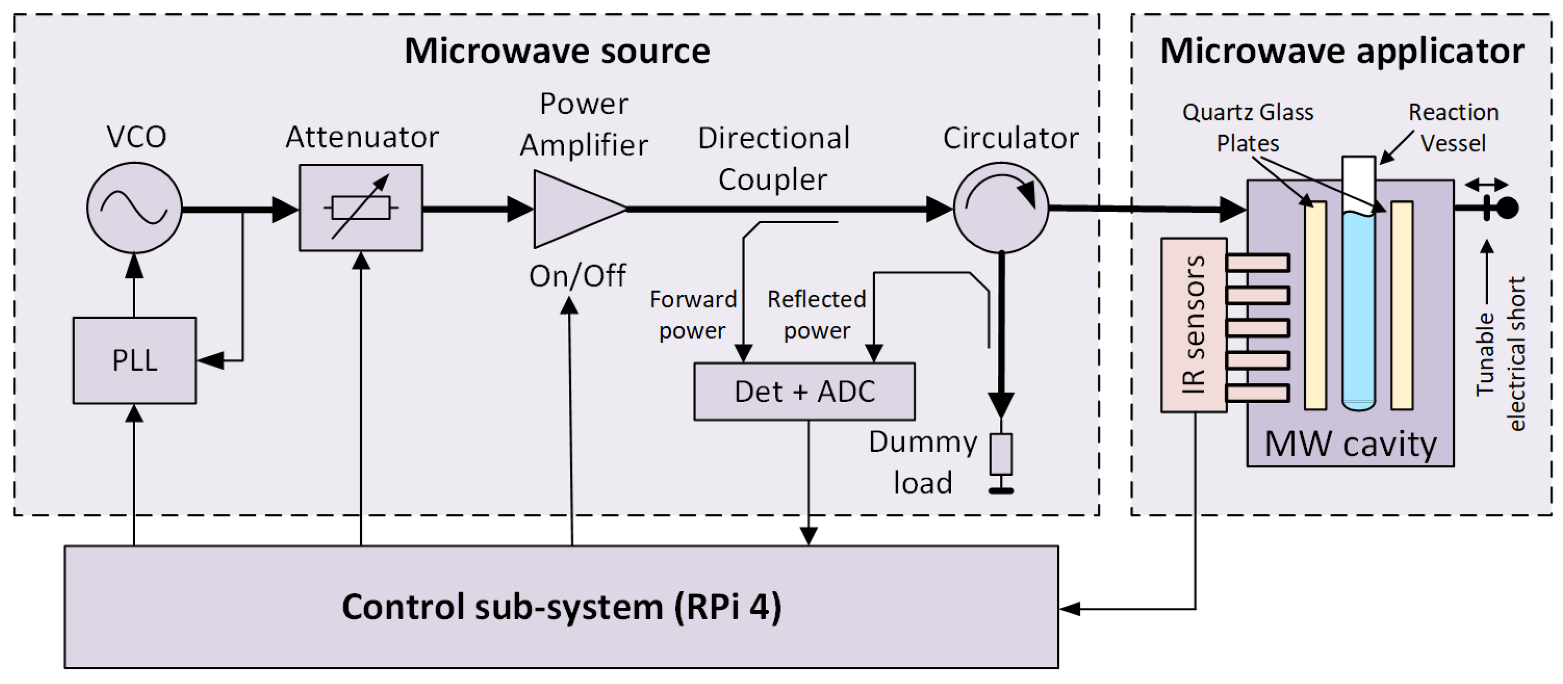
A block diagram of the microwave reactor is shown in Figure 1, and its photograph is presented in Figure 2. The reactor follows the general structure of such devices known from the literature [19] and consists of three main blocks: a microwave source, a microwave applicator, and a control sub-system.
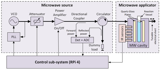
Figure 1.
A block diagram of the microwave reactor.
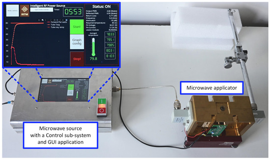
Figure 2.
A photograph of the microwave reactor.
The microwave source is designed as a cascade of several radio-frequency components. The first is a microwave synthesizer based on a voltage-controlled oscillator (VCO) coupled to a phase-locked loop (PLL). A low-power signal from the synthesizer is provided to a power amplifier via a tunable attenuator. The power amplifier is insulated against load changes using a circulator, which directs the reflected wave to a dummy load. Both forward and reflected power levels are measured using a pair of directional couplers and a power measurement block comprising logarithmic detectors and analog-to-digital converters (ADC). This way, the return loss of a load attached to the microwave source can be determined.
The central part of the microwave applicator is a microwave cavity [20], comprising a reaction vessel in the form of a typical laboratory tube. The cavity is a two-port network connected to the microwave source at the first port and a tunable electrical short at the second port. The tube is surrounded by impedance-matching plates made of quartz glass. Both the tube and the plates are held in place by supports made of Teflon to minimize loss (not shown in this figure for clarity). The plates and the correctly tuned electrical short ensure the desired microwave field distribution inside the reaction vessel. It should be noted that this distribution should be considered quasi-uniform and not literally uniform. The inner diameter of the tube corresponds to the wavelength at the desired operating frequency, assuming that the tube is filled with a substance characterized by a high electric permittivity ranging from 20 to 80. Therefore, the vessel almost acts as a dielectric resonator, and the presence of field minima and maxima disturbing the field’s uniformity inside its volume is inevitable. The temperature along the tube’s height is measured without contact using an array of infrared (IR) sensors. More information regarding the source and applicator, as well as the microwave field distributions in the correctly and poorly tuned reactor, can be found in Refs. [20,21]. The primary parameters of the reactor are presented in Table 1.

Table 1.
The primary parameters of the reactor.
The control sub-system is based on a Raspberry Pi 4 microcomputer. A dedicated driver monitors the current state and enables manual and automatic reactor control. Various system parameters and diagnostic data are tracked, the most important of which are the temperature values from all available sensors and the forward and reflected power levels from detectors. The driver can switch the power amplifier on or off, set the frequency of the microwave source, and set the attenuation of the tunable attenuator. The frequency is typically set once before the chemical reaction starts. However, the attenuation is used to tune the microwave power delivered to the cavity and, thereby, the temperature of the reacting mixture. In the automatic control mode, this is carried out using a software PID controller implemented as a part of the driver.
4. Results—The Software PID Controller and the Reactor Model
4.1. The Modeling Method
The PID controller model can be expressed by the following pseudo-code:
- Set the general algorithm parameters:
- time step: s
- mass of the tube: kg
- specific heat of the tube: J/kg/°C
- cooling factor: s−1
- temperature measurement delay: s
- standard deviation of the temperature measurement fluctuation:
- PID function call interval: s
- Set the parameters describing the specific experiment:
- mass of the substance to be heated:
- its specific heat:
- ambient temperature:
- desired temperature:
- switch-off time:
- Init variables:
- time index:
- initial power: W
- current temperature equal to the ambient temperature:
- Calculate the temperature change based on Equation (5) and
- Update the current temperature:
- Check whether the maximum heating time has elapsed:
- If , then and go to 8
- If seconds have passed since the last PID function call:
- i.
- Retrieve the temperature value with the account of the measurement delay:
- ii.
- Add some fluctuation:
- iii.
- Call the PID function to obtain the attenuation value:
- iv.
- Update the current power:
- Update the time index:
- Go to 4
The function denoted as realizes the operation of the PID controller given by
with substitutions (the current temperature, the process variable) and (the desired temperature, the setpoint). is the current error value and is an index of the current time instant. is a function that maps the desired power level onto corresponding attenuation (the controlled variable), is the current integral value, and , , and are the coefficients of the proportional, integral, and derivative terms, respectively. The switch-off time indicates when the heating process should be ended. stands for fluctuations generated according to the Gaussian distribution with zero mean and variance . All values are stored in double-precision floating-point variables to avoid problems with rounding and overflow.
The current temperature is calculated as an average over all temperature sensors. The mapping function is based on a lookup table containing power levels for all available attenuation settings from 0 to 31 dB. The controller defined by Equation (1) is able, at least theoretically, to track a time-varying setpoint. However, in this paper, only fixed setpoint cases are analyzed, which is stressed by omitting the time instant index in . The PID function is called every 1 s.
There are two objectives of the control: to keep the current temperature close to the setpoint and to keep the attenuation fixed. The latter objective is equivalent to keeping the microwave power fixed, which is advantageous for the reasons explained above. Deriving a PID controller configuration that meets both objectives requires the model to take into account the physical effects occurring in the microwave applicator during the heating process.
4.2. Microwave Absorption in the Cavity
From the point of view of microwave engineering, the cavity acts as a load for the microwave source. The impedance of this load depends on the tunable electrical short position and electrical properties of the reacting mixture, which may vary in temperature and time (due to the reaction progress). In a correctly tuned reactor, the return loss defined at the interface between the source and the cavity should be reasonably low the entire time the reaction proceeds.
Figure 3 shows the return loss at the cavity input port, measured in three cases where tap water was heated to various temperatures. The presented curves were obtained using the reactor’s capability of measuring the forward and reflected power levels and thus should be considered illustrative since the reactor was not designed to be a highly accurate reflectometer. However, one can see that the return loss is below −15 dB for lower temperatures, while for higher temperatures, it can reach approx. −8.5 dB. The lowest recorded value is −22.5 dB. This means that 0.5% to 14% of power may be reflected due to the impedance mismatch and lost in the dummy load. Since it was not possible to develop a simple model that would theoretically predict the value of the return loss based on the available information regarding the substances filling the reaction vessel, in the described reactor model, it is assumed that all the power delivered is dissipated in the microwave cavity, which obviously may decrease the modeling accuracy. The accurate calculation of the input reflection coefficient would require a thermal-electromagnetic FDTD simulation, which would complicate the model considerably. As the simplicity of the model was considered a more important objective than its absolute accuracy, it was decided to neglect the value of reflection losses.
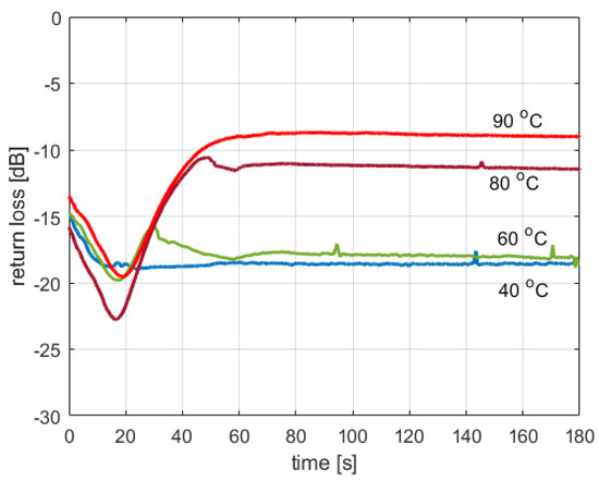
Figure 3.
Return loss in tap water heating experiments.
Microwaves penetrating the cavity can be absorbed by the elements of the cavity itself and by the reacting mixture. To maximize the reactor efficiency, the cavity was made of brass and the other elements of low-loss dielectric materials (the matching plates—quartz glass, the supports—Teflon, and the reaction vessel—laboratory glass). For this reason, the absorption by these elements is neglected, and in consequence, it is assumed that all the power dissipates in the reacting substances to be heated.
4.3. Heating and Cooling the Reacting Mixture
Let us consider that kilograms of a substance having a specific heat is placed in the reaction vessel, and the microwave source delivers temporary power . For a short time interval , one can express the temperature increase as
Equation (2) needs to be expanded by considering the presence of the reaction vessel, which is the main contributor to the inertia of temperature readings. Assuming that the vessel heats up fast as a result of being heated by its content, one can write the following:
where and are the vessel mass and specific heat, respectively. Other elements of the thermodynamic system (metal cavity, quartz glass impedance matching plates, etc.) have been omitted because, due to the low thermal conductivity of air and the large mass of the metal cavity, their influence on the overall system is marginal. On the other hand, their inclusion would complicate the model considerably.
The temperature drop due to heat being dissipated to the surroundings can be described using Newton’s law of cooling:
where is the current temperature of the substance of interest, is the ambient temperature, and the cooling factor that must be determined experimentally. The resultant temperature change is as follows:
Integrating the temperature changes calculated using Formulas (2)–(5) makes it possible to obtain the temperature course over an arbitrarily long period.
4.4. The Temperature Measurement Fluctuations
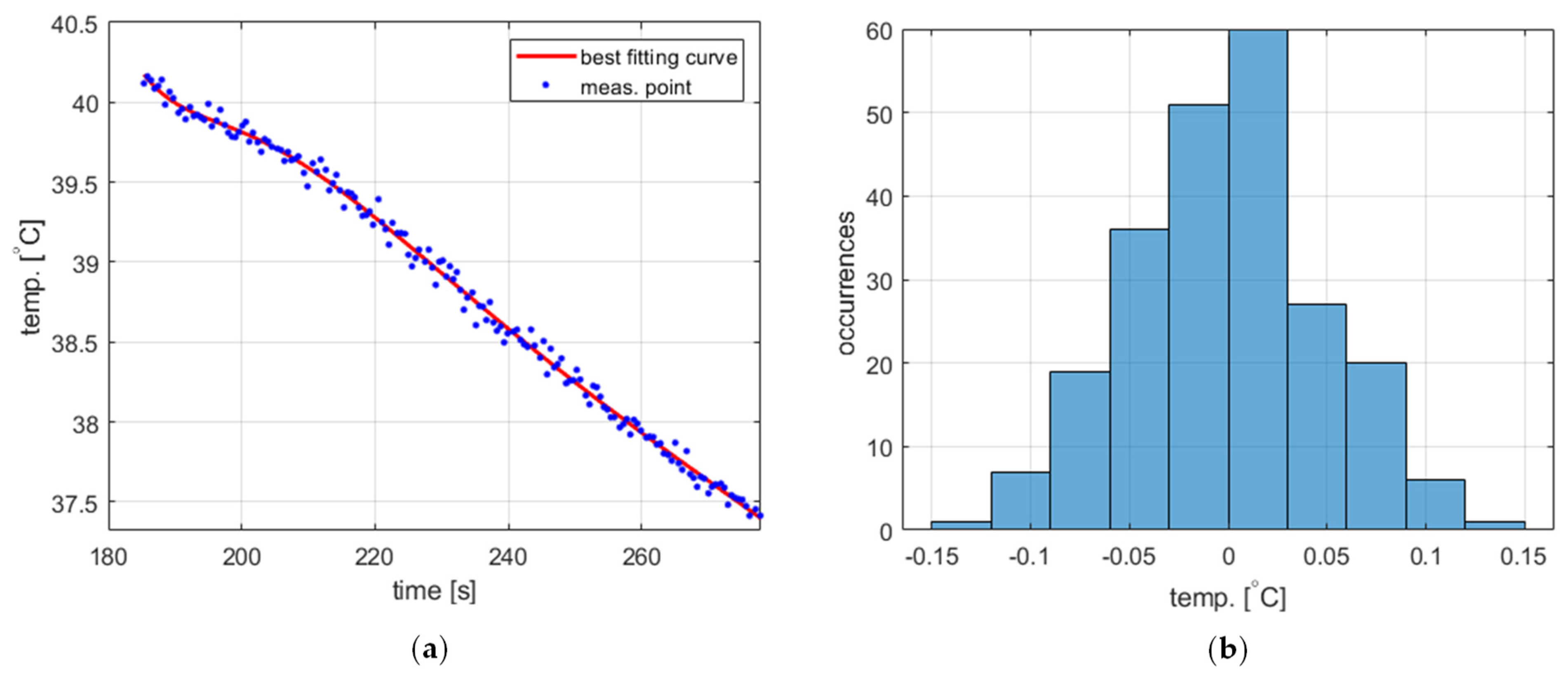
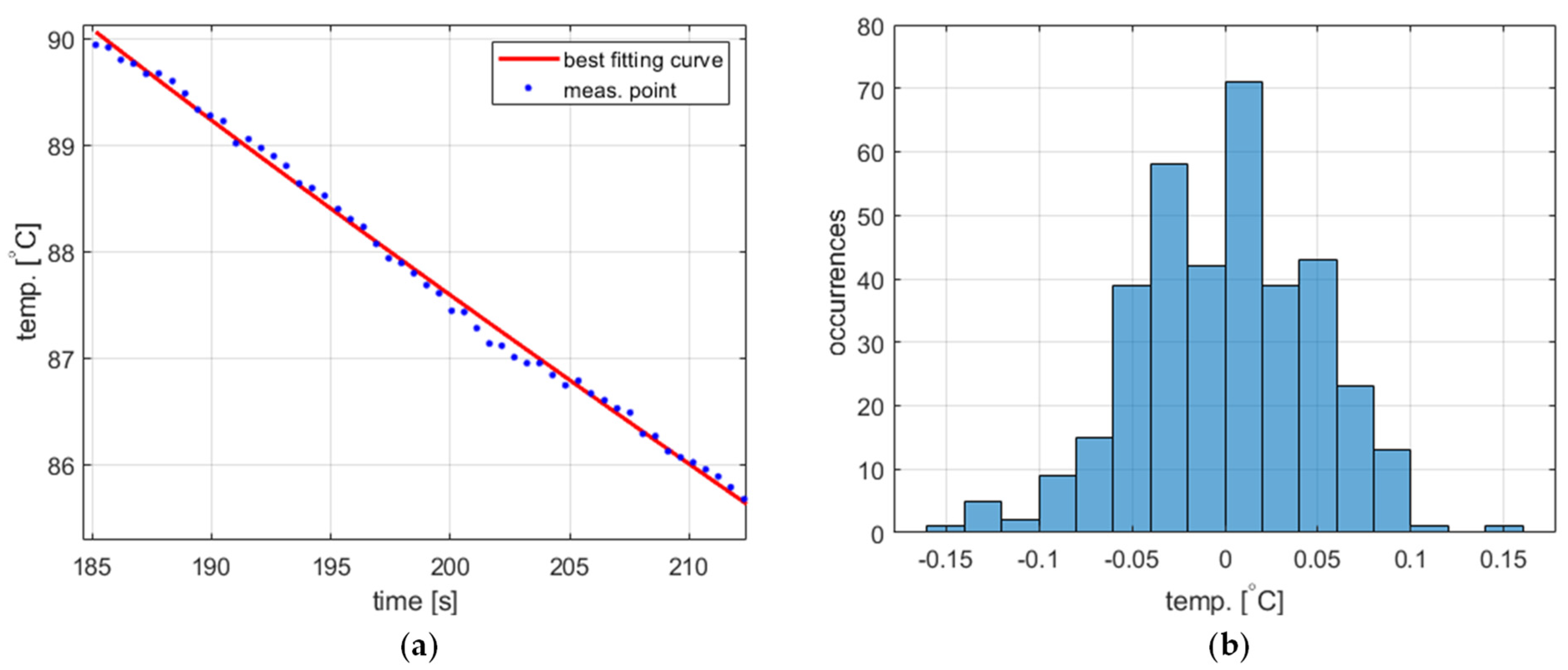
The temperature measurement performed to obtain the process variable value exhibits short-time fluctuations, which should be taken into account in the PID controller model. The statistical characteristics of these fluctuations were experimentally identified based on data obtained from two experiments, namely water cooling from 40 ° to 90 °C (Figure 4a and Figure 5a, respectively). The acquired temperature signals were decomposed into a monotonically decreasing component assumed to correspond to the actual cooling process and a rapidly time-varying component representing the fluctuations. The decomposition was carried out using the fit function available in Matlab R2023b environment [22] using the ninth-degree polynomial as a curve to fit. In both cases, the latter component was determined to have more or less Gaussian distribution (Figure 4b and Figure 5b) with a standard deviation of 0.0498 for 40 °C and 0.0490 for 90 °C. Accordingly, the temperature measurement fluctuations were assumed to be Gaussian-distributed for the entire PID model with a standard deviation of 0.05.
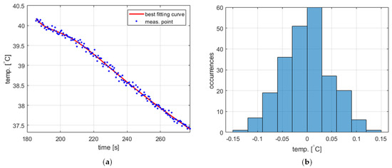
Figure 4.
The temperature measurement fluctuations for cooling from 40 °C, (a) measured temperature and the best fitting curve (zoomed for better visibility), and (b) the histogram of the fluctuations.

Figure 5.
The temperature measurement fluctuations for cooling from 90 °C, (a) measured temperature and the best fitting curve (zoomed for better visibility), and (b) the histogram of the fluctuations.
4.5. The Cooling Factor
Integrating Equation (4) makes it possible to express the cooling process using an exponential function of time:
where is the initial temperature. Thus, the cooling factor can be determined by finding , which provides the best fitting of the curve in Formula (6) for the experimental data.
Such a procedure was carried out using the aforementioned fit function for two data sets representing cooling tap water from both 90 °C and 60 °C (Figure 6). The results obtained were [s−1] and [s−1], respectively. As can be seen, they are different for different temperature ranges, and in both cases, the cooling process does not seem to follow the exponential function given by Equation (6) with high accuracy. This phenomenon has not been studied in depth. However, the obvious hypothesis is that the ambient temperature is not constant. The model developed assumes that the external environment for the tube is the inside of the cavity. Therefore, the ambient temperature corresponds to the air temperature inside the cavity. Due to the relatively small volume and lack of ventilation, air heats up when water in the tube is heated up to the initial temperature , and then cools down when the microwave source is turned off, starting the cooling process. Consequently, may differ from room temperature and vary over time.
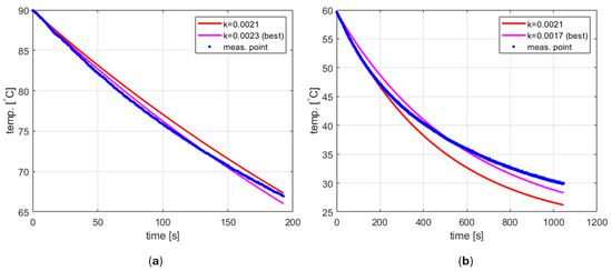
Figure 6.
The cooling process (a) starting from 90 °C, (b) starting from 60 °C.
Modeling changes in the ambient temperature is a complex problem that cannot be easily incorporated into the PID model due to unknown thermal resistance values between the tube and particular cavity elements. For this reason, it was decided to adopt a simplified approach in which the cooling process is described by Equation (6) with known and fixed and . The ambient temperature is easy to be determined using a thermometer. After several experiments, the cooling factor has been estimated and set to [s−1]. For the case shown in Figure 6a, this value results in a difference between the measured and calculated values of less than 1.5 °C. For the case of cooling from 60 °C, shown in Figure 6b, the difference reaches 4 °C. However, it should be noted that this occurs for relatively low temperatures, and for higher temperatures, the curve obtained fits the measurement data very well (actually better than the best curve). This may be advantageous because it is unlikely to use the reactor to carry out reactions that require a temperature close to the ambient one.
4.6. The Delay of the Temperature Measurement
As a result of volumetric heating in the microwave reactor, the content of the reaction vessel is heated up first, and only then does the temperature of the vessel itself increase. Since the contactless temperature sensors observe the walls of the vessel, temperature measurements are subject to a certain delay . This delay, in general, is problematic to determine due to the dependency on hard-to-define internal and external thermal boundary conditions. Thus, in the developed model, was experimentally estimated to be 4.5 s.
5. Discussion—Model Validation
The developed model was tested by comparing the temperature and power course obtained from the numerical simulation performed over time using the algorithm proposed above and the measurements performed in the microwave reactor. Unless expressly stated otherwise, the heated substance was 5 g of tap water. Such an amount completely fills the working part of the reaction vessel. The specific heat of water was assumed to be constant and set to [J/kg/°C].
5.1. The Effect of the Temperature Measurement Fluctuations
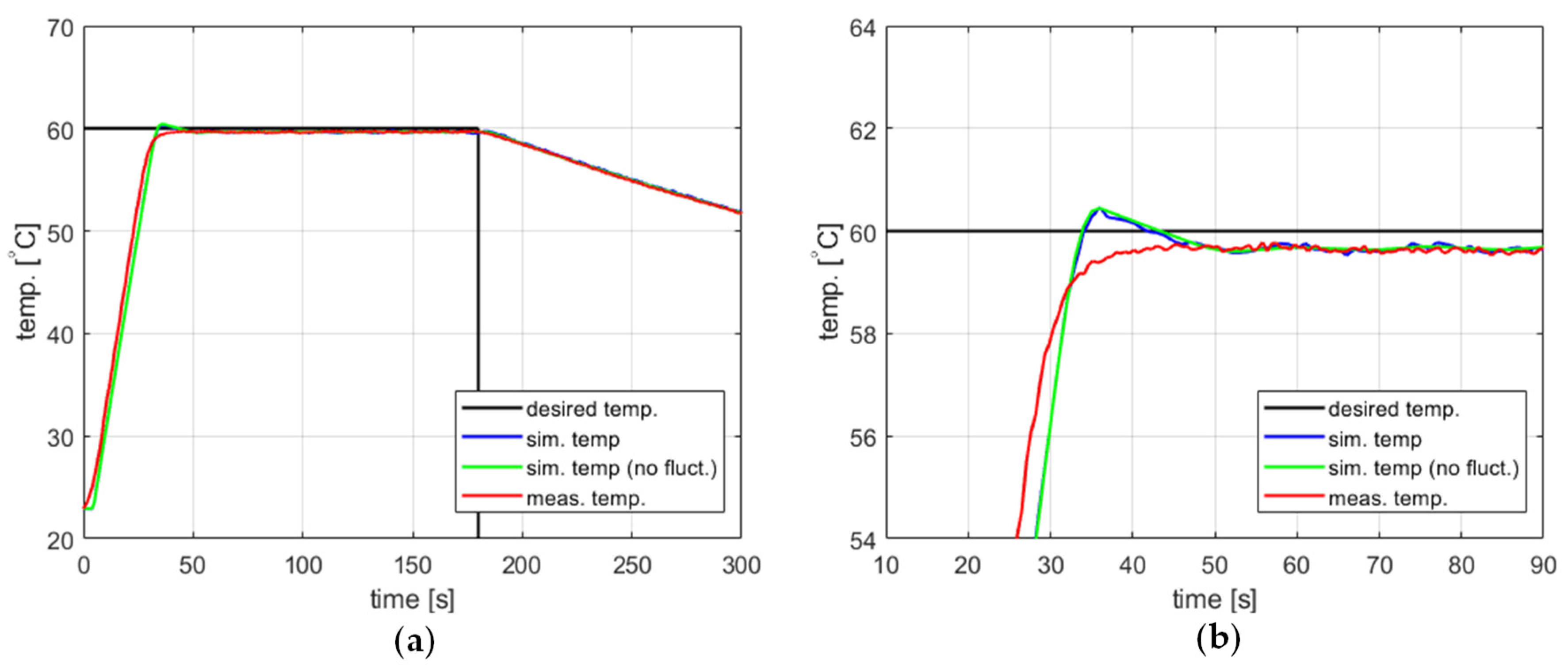
The impact of including temperature measurement fluctuations in the model on its accuracy can be demonstrated using the example of a PID controller with coefficients , , and and a setpoint of 60 °C. Figure 7 compares the measured and modeled behavior of such a controller, with and without the temperature measurement fluctuations taken into account. Curves for both the measured and simulated temperature over time seem to be reasonable for most applications. The steady-state error is approximately 0.5 °C. The model predicts a slight overshoot of about 0.6 °C, which does not occur in practice. Still, this fact has limited significance since the overshoot amplitude is comparable to the steady-state error. Also, it should be stressed that the model gives largely the same temperature response regardless of whether the temperature measurement fluctuations are or are not taken into account.
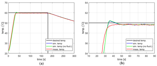
Figure 7.
The temperature over time for a heating process, , , , , (a) large-scale view, (b) zoomed-in view.
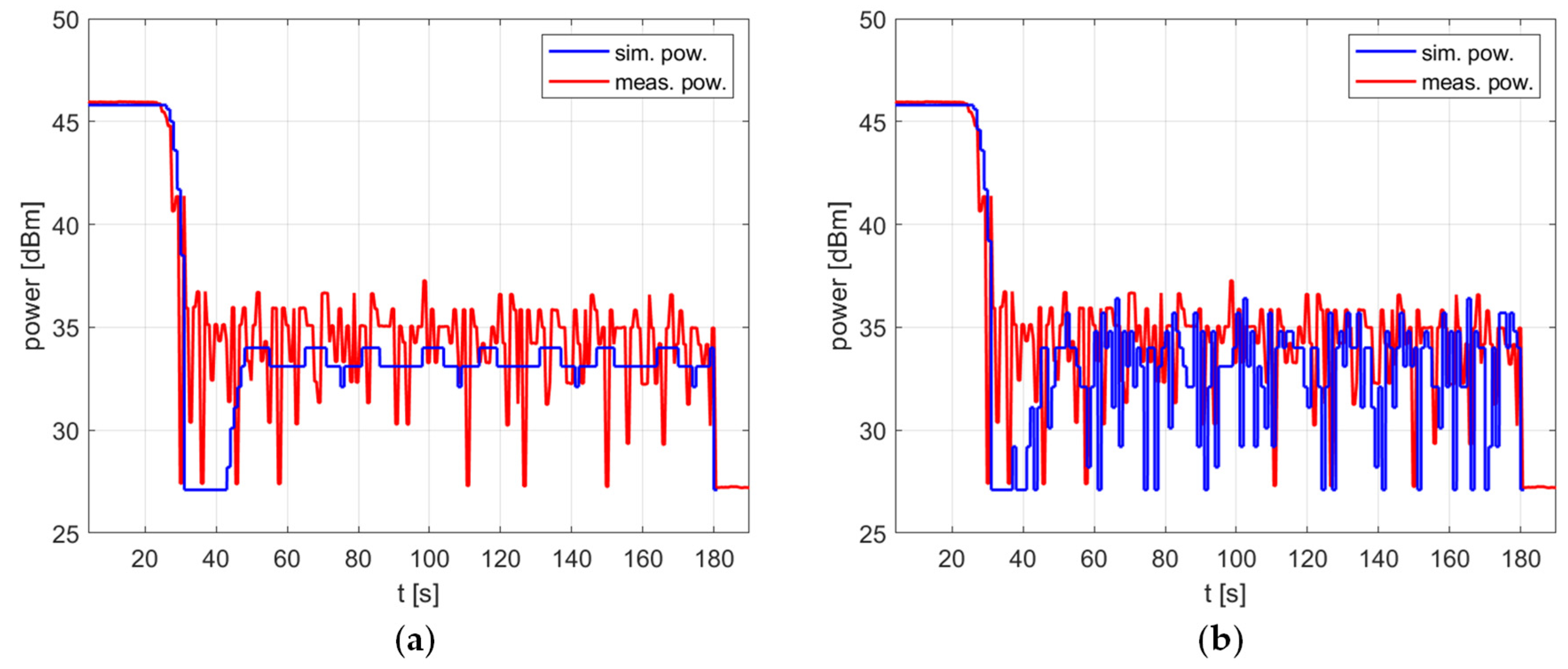
The impact of the temperature measurement fluctuations is clearly visible in Figure 8, which shows the delivered power level over time. For the case in which no fluctuations are taken into account, the simulated power can be considered almost fixed, which is advantageous for the reasons explained above. To be precise, after the overshoot is removed by switching the power off for a short time, the power oscillates periodically by 1 dB, with additional occasional drops of another 1 dB (Figure 8a). However, this steady state occurs in simulation only. In the experiment, the power rapidly changes within the range of 10 dB. To predict such a reactor behavior, one must introduce the temperature measurement fluctuation to the model. Figure 8b shows that after doing this, both the simulated and measured power exhibit changes of similar nature and range.

Figure 8.
The power over time for a heating process, , , , , (a) no temperature measurement fluctuations, (b) temperature measurement fluctuations included.
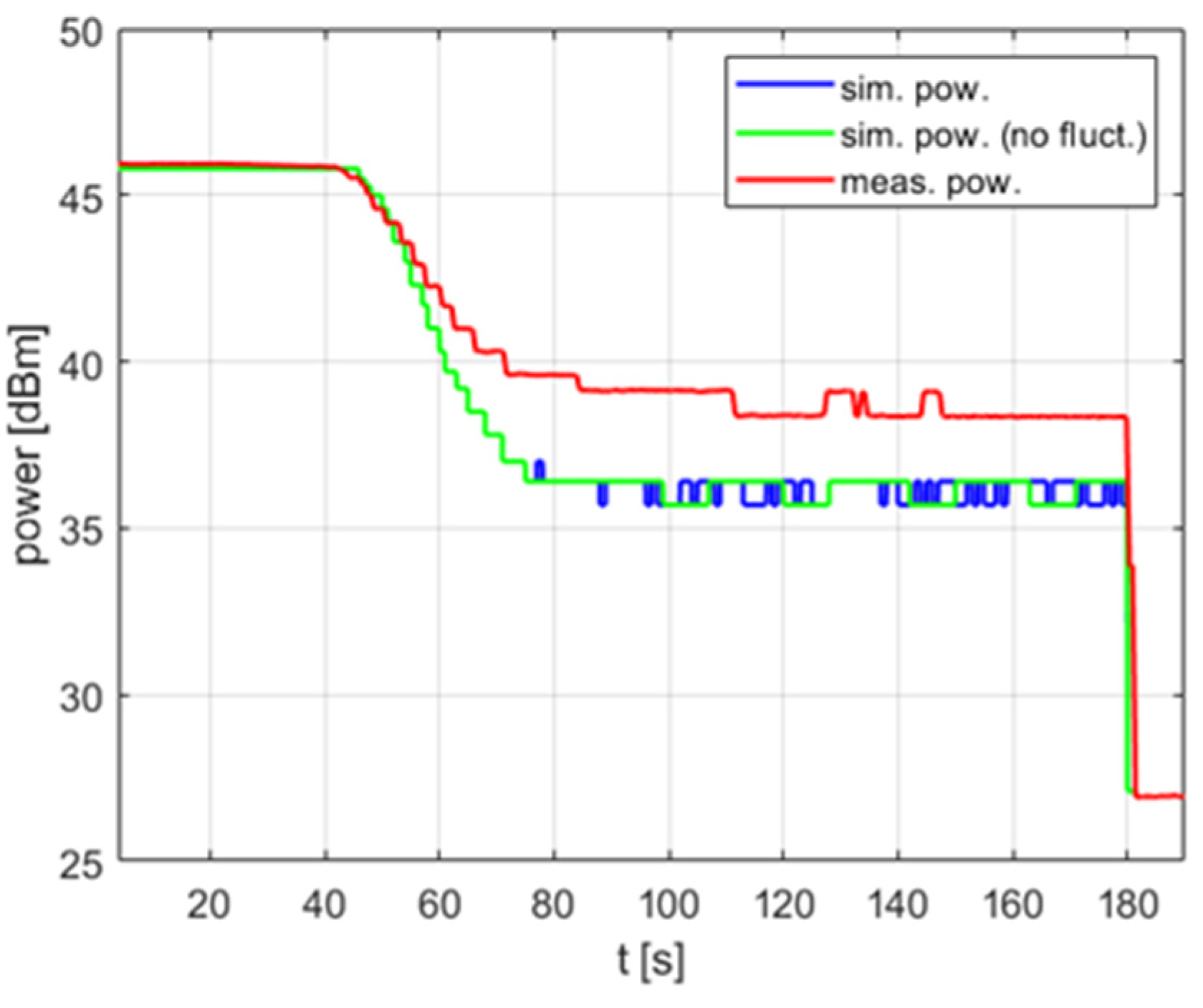
It is worth noting that the impact of the temperature measurement fluctuation is most visible in PID controllers with a non-zero derivative term . For PI (proportional–integral) controllers without a derivative term, omitting fluctuations in the model usually does not significantly reduce its accuracy, as shown in Figure 9. As can be seen, simulations with and without fluctuations result in the same delivered average power level and the same variations over time in the steady state. The measured power level exhibits similar variations but a slightly higher average value—this difference is discussed in the next section of the paper.
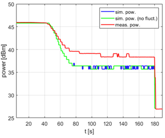
Figure 9.
The power over time for a heating process, , , , .
Moreover, since a constant power level is desired throughout the reaction, controller tuning usually results in . To fully utilize the PID controller capabilities, including the derivative term, one can attempt to adopt a technique known as a derivative filter. However, this technique has not been implemented in the reactor under test.
5.2. Controller Tuning for Various Setpoints
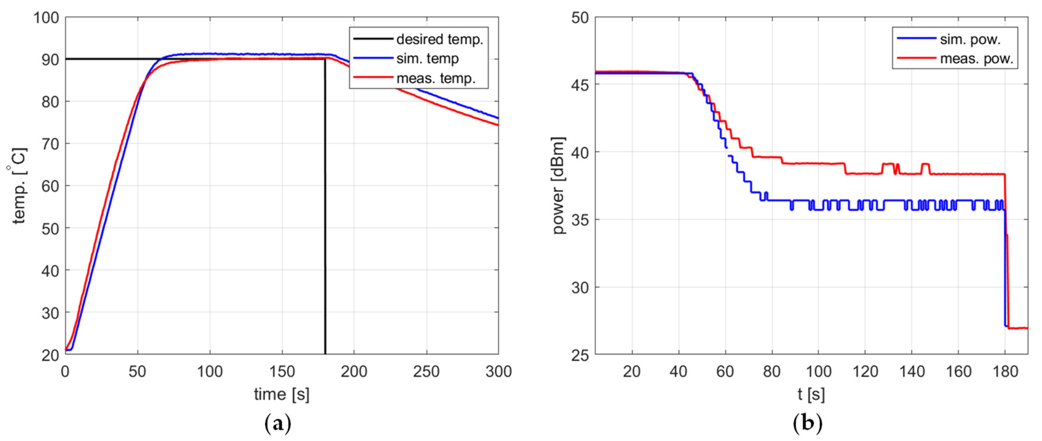
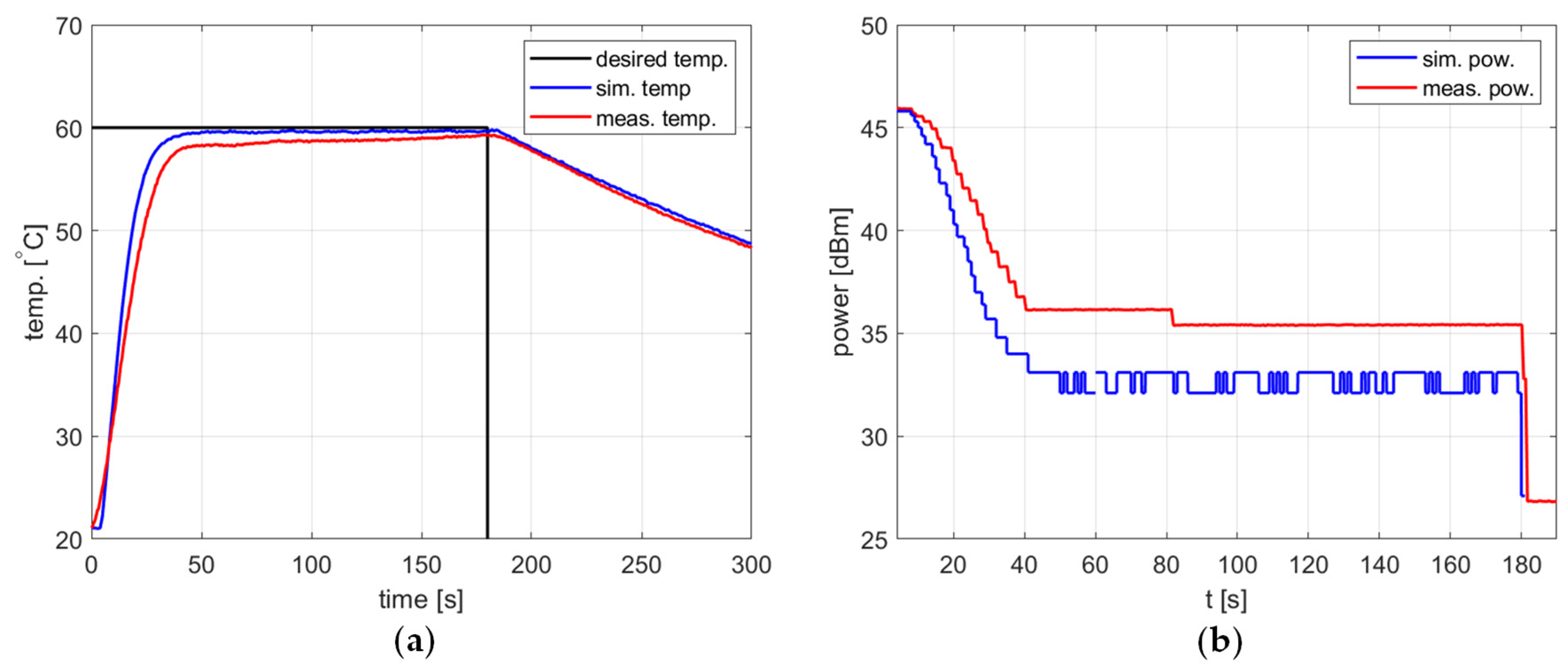
Figure 10, Figure 11 and Figure 12 and Table 2 refer to the simulation and measurement results obtained for heating processes with various setpoints. The PID controller coefficients were tuned for each setpoint using the developed model and the trial-and-error method. This was possible because the simulations based on the proposed algorithm allow one to obtain a PID response almost immediately without time-consuming experiments with actual water heating.
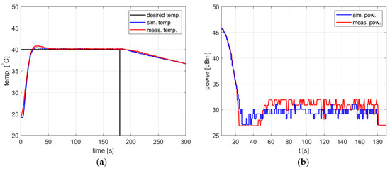
Figure 10.
Heating process, , , , , (a) the temperature over time, (b) power over time.
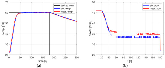
Figure 11.
Heating process, , , , , (a) the temperature over time, (b) power over time.
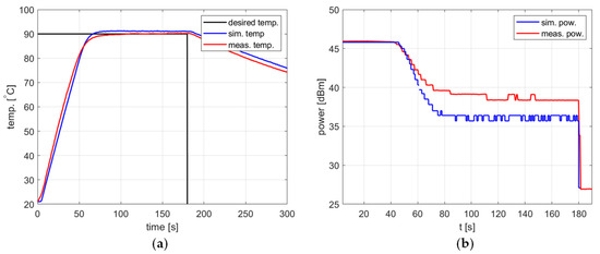
Figure 12.
Heating process, , , , , (a) the temperature over time, (b) power over time.
Table 2.
PID response characteristics.
In all presented cases, tuning aims were achieved, namely tracking the setpoint with a reasonable steady-state error and low power variations. The results obtained are summarized in Table 2.
In all cases, the simulation reflects the temperature course over time well. For a setpoint of 40 °C, the presence of an overshoot is correctly predicted, as is its amplitude. Also, the steady-state error and the rising time show good agreement between the simulation and measurement.
As for the power course over time, its general shape is well predicted, but its level is not. Figure 10, Figure 11 and Figure 12 show a difference of up to 4 dB between simulated and measured power levels. This is probably due to an over-reaching assumption about the heated substance’s total absorption of the delivered power. However, this is not a significant drawback of the model because the purpose of the PID controller is to provide a constant power level, not a set power level. An actual power level results from the temperature setpoint to be tracked.
5.3. Poorly Tuned Controller
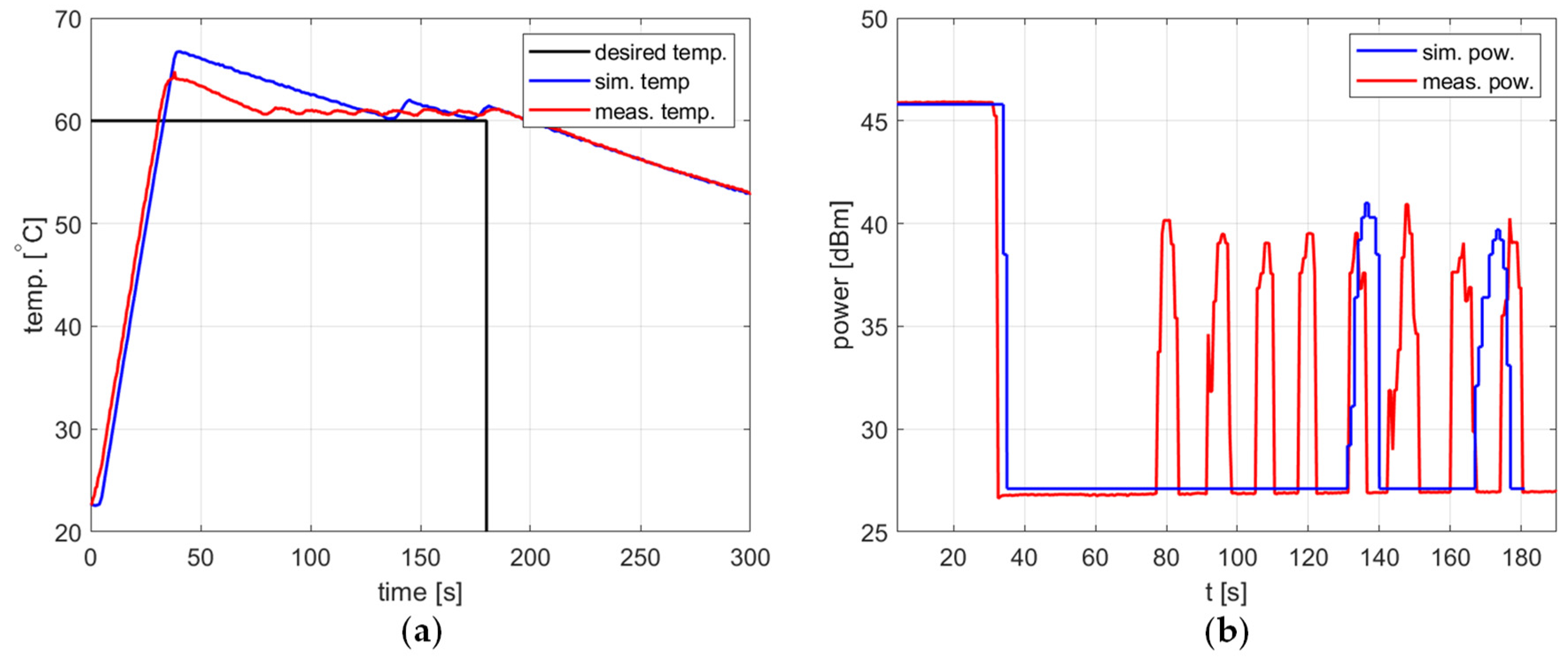
All the previously presented examples of the heating process relate to the correctly tuned controller, i.e., when the steady-state error is low, there are no oscillations, and the overshoot, if present, has limited amplitude. For all the cases, the agreement between the simulations and measurements is good enough to allow one to apply the determined PID coefficients in the reactor or use them as a good starting point for further fine-tuning. However, the investigation showed that the agreement was not so good in the case of a poorly tuned controller. An example of such a situation is presented in Figure 13. In the simulation, the temperature is significantly overshot and then exhibits decreasing oscillations. Similar behavior is observed in the measurements, but the overshoot is smaller and the oscillations are of a much lower amplitude, a much smaller period, and seem not to decrease. Figure 13b shows that peaks in the delivered power level occur in both the simulation and measurement, with a period corresponding to the period of temperature oscillations visible in Figure 13a. Accordingly, they occur more frequently in the measurements than in the simulation, and their amplitude is comparable.
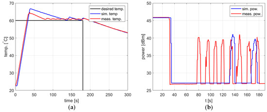
Figure 13.
Heating process for the poorly tuned controller, , , , , (a) the temperature over time, (b) power over time.
It should be emphasized that the practical significance of observed discrepancies is limited. In a typical situation, the model will be used to search for a PID controller configuration, resulting in the set temperature being appropriately tracked. The examples in the previous sections show that the discrepancies between the measurement and the model are significantly smaller.
5.4. Heating the Substance Other Than Water
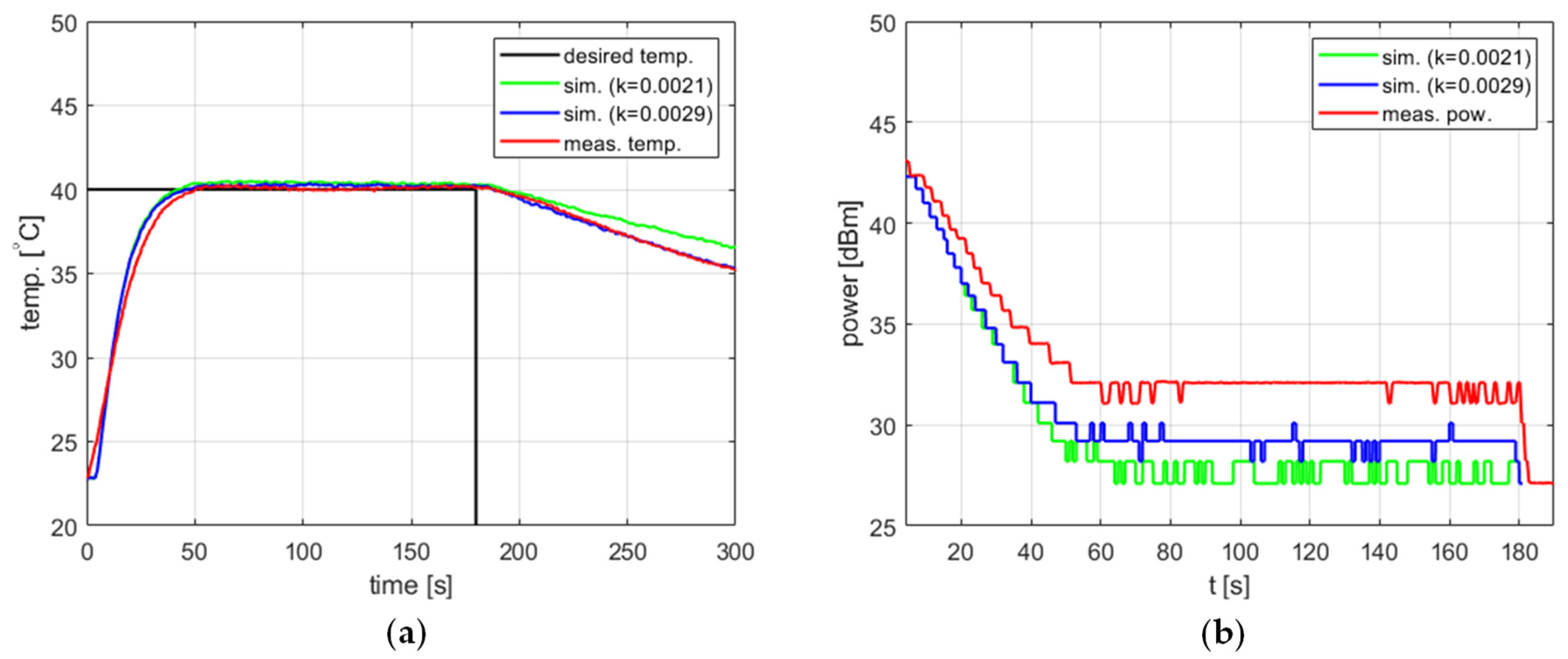
Since the parameters of the proposed model, i.e., the cooling coefficient, the amplitude of temperature measurement fluctuations, and the temperature measurement delay, were determined based on experiments using water, it should be checked whether the model also works for other substances. Such a test was performed using 4 g of 95% ethanol ( [J/kg/°C]). As in the case of water, the amount of ethanol was selected so as to fill the working part of the reaction vessel.
Figure 14 shows the results obtained for the setpoint , , , and . Two values of the cooling factor were tested, one determined for tap water ( [s−1]) and another one determined specifically for ethanol by repeating the experiments described above ( [s−1]). In both cases, the model confirmed its usefulness for tuning the PID controller. A reevaluation of resulted in the better modeling of the cooling process, a lower difference between the simulated and measured power level in the steady state, as well as a lower difference between the steady-state temperature errors. However, in the latter case, the improvement is of the order of 0.1 °C and is thus insignificant.
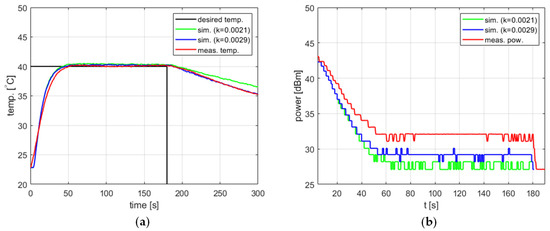
Figure 14.
Heating process for ethanol, , , , , (a) the temperature over time, (b) power over time.
Figure 15 shows the results of an experiment using ethanol in which the largest discrepancy between the simulation and measurement was observed. For the setpoint and the PID coefficients , , , the temperature in the simulation reaches the steady state, whereas in the measurement, it constantly increases slowly, and the steady state is not reached before the heating process ends. Nevertheless, the difference between the measured temperature and the setpoint does not exceed 2 °C and decreases with the progress of the heating process, which may be acceptable in many applications.
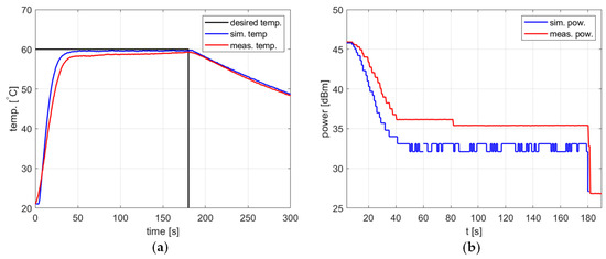
Figure 15.
Heating process for ethanol, , , , , (a) the temperature over time, (b) power over time.
6. Conclusions
In this paper, we proposed the model of a batch microwave reactor equipped with a software PID controller. The model allows one to obtain the coefficients of the PID controller in a quick and easy manner based mostly on numerical simulations, with a minimized number of time-consuming and potentially harmful tests using hot liquids.
The accuracy of the model is sufficient for many applications. In cases when exact temperature control is required, the results obtained from the model may constitute a good starting point for further fine PID controller tuning using experiments in actual hardware.
The proposed solution still needs to have some characteristics determined based on experimental data and optimization techniques. Some of them, like the distribution of temperature measurement fluctuations, can be assumed to be constant and must be determined only once. Others, such as the cooling factor, depend on the heated chemical reagent. Although it has been shown that using the cooling factor value determined for water for ethanol does not drastically reduce the accuracy of the model, this cannot be considered a rule that applies to any pair of substances. Nevertheless, using the presented model significantly limits the number of experiments to be performed for PID tuning.
The model is essentially based on known laws of physics. However, some phenomena were modeled in an extremely simplified way. All microwave power delivered by the microwave source was considered to penetrate the reaction vessel and dissipate in the heated substance. Cooling was assumed to take place at a fixed temperature. Furthermore, the heat transfer inside the reaction vessel and through its walls was only modeled by the temperature measurement delay with an experimentally selected value. Removing these simplifications requires further in-depth investigations.
Author Contributions
Conceptualization, S.K. and P.K.; methodology, S.K.; software, S.K. and P.K.; validation, P.K., W.W. and M.B.; formal analysis, S.K. and W.W.; investigation, S.K.; resources, P.K. and M.B.; data curation, S.K.; writing—original draft preparation, S.K.; writing—review and editing, W.W., P.K. and M.B.; visualization, P.K.; supervision, W.W.; project administration, P.K.; funding acquisition, W.W. All authors have read and agreed to the published version of the manuscript.
Funding
The research was funded by Warsaw University of Technology within the Excellence Initiative: Research University (IDUB) program (BEYOND-POB 1820/54/Z01/2021).
Data Availability Statement
The data used in the presented research are available from the authors upon a reasonable request.
Acknowledgments
The authors acknowledge Dariusz Kołodziej (Warsaw University of Technology) for his assistance with mechanical design of the microwave applicator and its CNC fabrication. The authors acknowledge Adrian Kruczak (Warsaw University of Technology) for the help in GUI application design.
Conflicts of Interest
The authors declare no conflicts of interest. The funders had no role in the design of the study; in the collection, analyses, or interpretation of data; in the writing of the manuscript; or in the decision to publish the results.
References
- Osepchuk, J.M. A History of Microwave Heating Applications. IEEE Trans. Microw. Theory Technol. 1984, 32, 1200–1224. [Google Scholar] [CrossRef]
- Sun, J.; Wang, W.; Yue, Q. Review on Microwave-Matter Interaction Fundamentals and Efficient Microwave-Associated Heating Strategies. Materials 2016, 9, 231. [Google Scholar] [CrossRef] [PubMed]
- Horikoshi, S.; Schiffmann, R.F.; Fukushima, J.; Serpone, N. Microwave Chemical and Materials Processing, 1st ed.; Springer Nature: Singapore, 2018; pp. 183–373. [Google Scholar] [CrossRef]
- Mohabeer, C.; Guilhaume, N.; Laurenti, D.; Schuurman, Y. Microwave-Assisted Pyrolysis of Biomass with and without Use of Catalyst in a Fluidised Bed Reactor: A Review. Energies 2022, 15, 3258. [Google Scholar] [CrossRef]
- Gerbec, J.A.; Magana, D.; Washington, A.; Strouse, G.F. Microwave-enhanced reaction rates for nanoparticle synthesis. J. Am. Chem. Soc. 2005, 127, 15791–15800. [Google Scholar] [CrossRef] [PubMed]
- Shibatani, A.; Matsumura, S.; Asakuma, Y.; Saptoro, A. Promoting Nucleation in Microwave-Assisted Nanoparticle Synthesis Using Combined Two-Stage Irradiation and Anti-Solvent Addition. Crys. Res. Technol. 2019, 54, 1800205. [Google Scholar] [CrossRef]
- Bálint, E.; Tajti, Á.; Keglevich, G. Application of the Microwave Technique in Continuous Flow Processing of Organophosphorus Chemical Reactions. Materials 2019, 12, 788. [Google Scholar] [CrossRef] [PubMed]
- Priecel, P.; Lopez-Sanchez, J.A. Advantages and Limitations of Microwave Reactors: From Chemical Synthesis to the Catalytic Valorization of Biobased Chemicals. ACS Sustain. Chem. Eng. 2019, 7, 3–21. [Google Scholar] [CrossRef]
- Nain, S.; Singh, R.; Ravichandran, S. Importance of Microwave Heating in Organic Synthesis. Adv. J. Chem. 2019, 2, 94–104. [Google Scholar] [CrossRef]
- Antonio, C.; Deam, R.T. Can ‘microwave effects’ be explained by enhanced diffusion? Phys. Chem. Chem. Phys. 2007, 9, 2976–2982. [Google Scholar] [CrossRef] [PubMed]
- Lew, A.; Krutzik, P.O.; Hart, M.E.; Chamberlin, A.R. Increasing Rates of Reaction: Microwave-Assisted Organic Synthesis for Combinatorial Chemistry. J. Comb. Chem. 2002, 4, 95–105. [Google Scholar] [CrossRef] [PubMed]
- Åström, K.J.; Hägglund, T. PID Controllers: Theory, Design and Tuning, 2nd ed.; Instrument Society of America: Pittsburgh, PA, USA, 1995. [Google Scholar]
- O’Dwyer, A. Handbook of PI and PID Controller Tuning Rules, 3rd ed.; Imperial College Press: London, UK, 2009. [Google Scholar]
- Ziegler, J.G.; Nichols, N.B. Optimum settings for automatic controllers. Trans. ASME 1942, 64, 759–768. [Google Scholar] [CrossRef]
- Cohen, G.H.; Coon, G.A. Theoretical Consideration of Retarded Control. Trans. ASME 1953, 75, 827–834. [Google Scholar] [CrossRef]
- Veronesi, M.; Visioli, A. On the Selection of Lambda in Lambda Tuning for PI(D) Controllers. IFAC-PapersOnLine 2020, 53, 4599–4604. [Google Scholar] [CrossRef]
- Bashishtha, T.K.; Singh, V.P.; Yadav, U.K.; Varshney, T. Reaction Curve-Assisted Rule-Based PID Control Design for Islanded Microgrid. Energies 2024, 17, 1110. [Google Scholar] [CrossRef]
- Zeng, D.; Zheng, Y.; Luo, W.; Hu, Y.; Cui, Q.; Li, Q.; Peng, C. Research on Improved Auto-Tuning of a PID Controller Based on Phase Angle Margin. Energies 2019, 12, 1704. [Google Scholar] [CrossRef]
- Olszewska-Placha, M.; Gryglewski, D.; Wojtasiak, W.; Celuch, M. Demonstration of a Combined Active-Passive Methodology for the Design of Solid-State-Fed Microwave Ovens. In Proceedings of the 18th International Conference on Microwave and High Frequency Applications AMPERE, Gothenburg, Sweden, 13–16 September 2021. [Google Scholar]
- Gwarek, W.; Jankowski, K.; Wojtasiak, W.; Borowska, M.; Korpas, P.; Kozłowski, S.; Gryglewski, D.; Kołodziej, D. Aplikator Mikrofalowy do Przeprowadzania Reakcji Chemicznych. Polish Patent 244854, 11 March 2024. Available online: https://api-ewyszukiwarka.pue.uprp.gov.pl/api/collection/749039c36da775a0df0ff024830b480c (accessed on 1 July 2024).
- Korpas, P.; Borowska, M.; Celuch, M.; Gryglewski, D.; Jankowski, K.; Kozłowski, S.; Wojtasiak, W. A Reactor for Microwave-Assisted Chemistry. IEEE Microwave Magazine accepted.
- Matlab Help Center. “Fit” Function Documentation. Available online: https://www.mathworks.com/help/curvefit/fit.html (accessed on 1 June 2024).


Disclaimer/Publisher’s Note: The statements, opinions and data contained in all publications are solely those of the individual author(s) and contributor(s) and not of MDPI and/or the editor(s). MDPI and/or the editor(s) disclaim responsibility for any injury to people or property resulting from any ideas, methods, instructions or products referred to in the content. |
© 2024 by the authors. Licensee MDPI, Basel, Switzerland. This article is an open access article distributed under the terms and conditions of the Creative Commons Attribution (CC BY) license (https://creativecommons.org/licenses/by/4.0/).