Research on Energy-Saving Control Strategies for Single-Effect Absorption Refrigeration Systems

Abstract

The automatic control device is a critical component of absorption refrigeration systems. Its functional enhancement can reduce operating costs, improve energy efficiency, and ensure long-term stable unit operation. Given that absorption refrigeration systems operate under various dynamic conditions, the rational design of control strategies is particularly important. This study analyzes the influence of changes in the cooling water and heat source water flow rates on the outlet temperature of chilled water in the unit based on the open-loop response characteristics of absorption refrigeration systems. It proposes a dual-loop energy-saving control strategy for single-effect hot water lithium bromide absorption refrigeration systems based on the setpoint comprehensive optimization algorithm. Considering the multiple variables, strong coupling, large inertia, long time delay, and nonlinear characteristics of absorption refrigeration systems, as well as the difficulties in modeling these systems, this study applies a model-free adaptive control algorithm to the system’s control. It derives both SISO and MIMO model-free control algorithms with time-delay components. Through simulations comparing MFAC, improved MFAC, and traditional PID control, the dual-loop energy-saving control strategy is demonstrated to effectively reduce system heat consumption by approximately 20%, decrease power consumption by about 10%, and enhance the system’s SCOP by approximately 19.3%.

1. Introduction

Absorption refrigeration originated in 1810, with the creation of the first intermittent absorption refrigeration unit by the Scotsman John Leslie. Fifty years later, the Frenchman Ferdinand Carré invented a continuous ammonia–water absorption refrigeration unit and obtained a U.S. patent for it [1]. In 1976, B.C.L. (Battelle Columbus Laboratories) in the United States proposed the concept of the absorption heat pump and conducted market forecasts that confirmed the practical value of absorption heat pump technology.

Similar to vapor compression refrigeration, absorption refrigeration also achieves cooling by evaporating the refrigerant at a low pressure to absorb heat after it has been throttled and depressurized from a high-pressure liquid state. The primary difference between the two methods lies in how the low-pressure refrigerant vapor is converted into high-pressure vapor. Vapor compression refrigeration uses an engine-driven compressor powered by electricity, whereas absorption refrigeration utilizes a “quasi-compressor subsystem” consisting of an absorber, a solution pump, and a generator, consuming thermal energy to achieve this conversion.

The application of absorption refrigeration systems has a history spanning several decades. However, their relatively low energy efficiency has been a key limiting factor for their widespread adoption. Regarding primary energy utilization efficiency, single-effect absorption refrigeration units have a coefficient of performance (COP) of approximately 0.6 to 0.8 and double-effect units of about 1.0 to 1.2, significantly lower than the COP of mainstream air compression refrigeration systems in the current air conditioning market. To enhance the performance of absorption refrigeration systems, numerous scholars domestically and internationally have conducted extensive research on optimizing units’ structural design [2,3,4,5,6], improving heat exchanger performance [7,8], and exploring new working fluid pairs [9,10]. However, much of this work has focused on the design and development stages of the units, with relatively limited research on further improving the energy efficiency of constructed equipment through control methods. Existing control methods can be broadly categorized into traditional, feedback, and intelligent and optimized control.

1.1. Traditional Control

Early research on controlling absorption refrigeration systems primarily focused on simple start or stop control, open-loop control, and thermal optimization. D. Didion et al. [11] studied the relationship between ambient temperature and unit load during on or off operation and proposed a start/stop control scheme for refrigeration units. S. Alvares et al. [12] found that, due to the thermal inertia effect, start or stop control typically leads to a decrease in system efficiency.

1.2. Feedback Control

With the development of sensor and detection technologies, feedback control has been widely applied in the control of absorption refrigeration systems. Currently, most absorption refrigeration systems use a single-loop control strategy, with the chilled water outlet temperature as the controlled variable. Chen et al. [13] proposed a computer monitoring and closed-loop control strategy for ammonia–water absorption heat pumps, which involves adjusting the flow rates of the refrigerant, dilute solution, and cooling water through control valves. This control scheme enables automatic start/stop and online control of the unit. K.L. Cézara et al. [14] successfully developed a closed-loop PID control system, based on the Arduino platform, which effectively prevented crystallization by optimizing the flow control of water and a LiBr/H₂O salt solution, achieving cost effectiveness and optimized operating conditions. Staudt S. et al. [15] showed that two MIMO control approaches (the proposed state feedback and the MPC approach) allow for a wider operating range and, hence, better part load capability compared to the SISO PI control approach. While MPC generally results in a comparably high computational effort due to the necessity of continuously solving an optimization problem, the proposed state feedback control approach is mathematically simple enough to be implemented in a conventional programmable logic controller.

1.3. Intelligent and Optimized Control

In recent years, with the development of artificial intelligence, scholars have gradually introduced machine learning algorithms, such as artificial neural networks and genetic algorithms, into the modeling and control of absorption refrigeration units. J. Labus et al. [16] demonstrated a control strategy based on inverse artificial neural networks that can accurately estimate key operating variables of small absorption refrigeration units within 25 s, achieving the high-precision control of cooling loads and providing an efficient and low-error solution for online systems. Suellen Cristina Sousa Alcântara et al. [17] combined neural networks and genetic algorithms to predict the transient performance of absorption refrigeration units. They trained neural networks to predict system responses using data and optimized them with genetic algorithms to improve accuracy. Tang C. et al. [18] proposed a predictive control model of regional cooling systems, which was conducive to improving the flexibility of the system alongside its peak-shifting and valley-filling abilities. In this model, an artificial bee colony (ABC)-optimized back-propagation (BP) neural network was used to predict the cooling load of the regional cooling system, and model parameter identification was adopted, combining the use of a river water-source heat pump and ice-storage technology. Homod R. Z. et al. [19] proposed a novel approach, using multiagent deep clustering reinforcement learning (MADCRL) to optimize load-shifting within multi-tank chilled water (MTCW) systems. The core of this approach lies in the MADCRL policy, which intelligently sequences chiller operations by taking advantage of cooler night-time temperatures.

There has been considerable research on the optimization of absorption refrigeration systems [20,21,22,23], but it has mainly focused on optimizing systems’ COP, heat transfer area, and operating costs based on thermodynamic principles under design conditions. J. Marcos et al. [24] demonstrated, through extensive experiments, that increasing the condenser and absorber temperatures or the degassing range of the lithium bromide solution could significantly improve the COP of refrigeration systems.

1.4. Current Research

Existing control schemes for absorption refrigeration systems have certain limitations. Single-loop control schemes can only meet the cooling capacity demand of the system but cannot ensure system efficiency. PID controllers perform poorly in adjusting for the large inertia and long time delays of absorption refrigeration systems. Most advanced control algorithms depend highly on precise mathematical models of the controlled object, and the complex operating mechanisms of absorption refrigeration systems make it difficult to establish accurate system models. Even the simplified mathematical models often fail to accurately describe the system state and cannot be used for controller design, being more suited for system characteristic analysis.

This study focuses on a 5.5 kW hot-water single-effect lithium bromide absorption refrigeration unit, aiming to explore a dual-loop energy-saving control strategy based on system analysis. This scheme uses the cooling water flow rate and the heat source water flow rate as the operating variables, with the unit’s chilled water outlet temperature as the main control variable and the generator’s temperature as an auxiliary control variable, aiming to achieve further energy-saving control of the absorption refrigeration system based on setpoint comprehensive optimization. The single-loop and dual-loop energy-saving control strategies of the absorption refrigeration system were simulated, and the study showed that the latter can effectively reduce the system’s heat consumption, decrease power consumption, and improve the system’s SCOP. The final experiments also proved the feasibility of the control algorithm. At the same cooling capacity of 3.276 kW, compared to single-loop control, the dual-loop control strategy reduced heat consumption by about 20%, power consumption by about 10%, unit COP by 16.6%, and the overall system SCOP by 16.6%.

2. System Description

2.1. Overview of an Absorption Refrigeration System

As shown in Figure 1, a complete absorption refrigeration system primarily consists of the absorption refrigeration unit and three peripheral circuits: the heat source, cooling, and chilled water circuits. The absorption refrigeration unit is the core of the entire refrigeration system, producing the required cooling capacity for users. The heat source circuit (indicated by the red line) provides the necessary thermal energy for the operation of the refrigeration unit. The cooling water circuit (indicated by the green line) removes the heat generated during the unit’s refrigeration process, discharging it into the environment through an outdoor cooling tower. The chilled water circuit (indicated by the blue line) delivers the cooling capacity of the unit to the users, cooling the indoor environment through terminal air conditioning equipment such as fan coil units. The circulation in the three peripheral circuits is driven by pumps installed on the piping of each circuit. Different heat pumps and pipes can affect system operation, and heat pipes with high thermal conductivity are beneficial for improving the overall thermal performance of the system [25], playing an important role by ensuring the smooth operation of the entire control system [26].

2.2. Working Fluid Pair in Absorption Refrigeration

The working fluid used in absorption refrigeration units is a binary solution composed of two substances with different boiling points that can dissolve into one another, commonly referred to as the “working pair”. The solution’s ability to evaporate the low-boiling-point component under certain conditions and strongly absorb the low-boiling-point vapor under others completes the refrigeration cycle. The substance with the higher boiling point is typically called the absorbent, while the other is the refrigerant [27].

2.3. Thermodynamic Analysis of the Absorption Refrigeration Cycle

Absorption refrigeration units operate by transferring heat from a low-temperature environment to a high-temperature environment under the driving force of a heat source [28]. Throughout the entire unit, only the solution pump consumes a small amount of electrical energy to drive the solution’s circulation. The thermodynamic analysis of absorption refrigeration systems involves the application of the law of mass conservation, component conservation equations, and the first and second laws of thermodynamics [29,30,31,32].

Mass conservation:

$${\displaystyle \sum {\dot{m}}_i}={\displaystyle \sum {\dot{m}}_o}$$

(1)

Component conservation:

$${\displaystyle \sum {\dot{m}}_i{X}_i}={\displaystyle \sum {\dot{m}}_o{X}_o}$$

(2)

The essence of the first law of thermodynamics is the energy conservation equation, which states that different energies can be converted into each other, with the total value of energy remaining constant in the conversion process:

$${\displaystyle \sum \dot{Q}}-{\displaystyle \sum \dot{W}}={\displaystyle \sum {\dot{m}}_o{h}_o-{\displaystyle \sum {\dot{m}}_i{h}_i}}$$

(3)

An absorption refrigeration system’s performance can be characterized by its coefficient of performance (COP), which is defined as the ratio of the system’s cooling capacity to the energy consumed:

$$COP={\displaystyle \frac{{\dot{Q}}_{eva}}{{\dot{Q}}_{gen}+{\dot{W}}_{pump}}}$$

(4)

The process of energy transfer in nature has directionality, and refrigeration cannot occur spontaneously. Absorption refrigeration units need to produce cooling by consuming heat. The second law of thermodynamics further states that the conversion efficiency between energies is affected by the quality of energy, and only a portion of it can be converted into useful work, usually referred to as effective energy:

$$\Delta \psi ={\displaystyle \sum {\dot{m}}_i{\psi }_i-{\displaystyle \sum {\dot{m}}_o{\psi }_o}\pm {\displaystyle \sum \dot{Q}\left(1-\frac{T_0}{T}\right)}}\pm {\displaystyle \sum \dot{W}}$$

(5)

Here, ${\dot{m}}_i$ represents the fluid mass flow rate at the inlet and outlet of each component in the system (kg/s); $X_i$ represents the mass fraction of fluid entering and exiting each component of the system; $h_i$ represents the inlet and outlet fluid enthalpy values of various components in the system (kJ/kg); $\dot{Q}$ represents the heat transfer rate of each component in the system (kJ/s); $\dot{W}$ represents external work for the system or the work required to apply power on the system (kW); $\Delta \psi$ represents the system’s effective energy loss (kJ/s); ${\psi }_i$ represents the effective energy of fluid at the inlet and outlet of each component in the system (kJ/kg); $T_0$ represents the ambient temperature (°C); and $T$ represents the temperature of each component (°C).

During the operation of an absorption refrigeration system, all components of the unit continuously exchange heat, such as the shell-side solution and tube-side heat source in the generator, the shell-side refrigerant and tube-side cooling water in the condenser, the shell-side refrigerant and tube-side chilled water in the evaporator, the shell-side solution and tube-side cooling water in the absorber, and the heat transfer between the cold and hot solutions on both sides of the solution heat exchanger. There is a relationship between the heat transfer rate of each component, defined as follows:

$$\dot{Q}=U\cdot A\cdot \Delta T$$

(6)

Here, $U$ represents the heat transfer coefficient (W/(m²·K)); $A$ represents the heat transfer area (m²); and $\Delta T$ represents the heat transfer temperature difference, calculated using the logarithmic mean temperature difference in the text (°C).

This study used the centralized parameter method to establish a dynamic model of the heat exchanger. In order to simplify the model’s structure and facilitate subsequent solving, the following assumptions were adopted in the modeling process of the hot water single-effect lithium bromide absorption refrigeration system:

• The generator, condenser, evaporator, and absorber were modeled using the lumped parameter method. The working medium inside the heat exchanger was in a dynamic-phase equilibrium state, with uniform temperature, pressure, and solution concentration at each point;
• The condensation pressure was equal to the occurrence pressure, and the evaporation pressure was equal to the absorption pressure;
• We neglected the heat exchange between the unit and the surrounding environment;
• We neglected the decrease in pipe pressure caused by pipeline length and resistance;
• The power of the solution pump was very small and could be ignored;
• The inlet cooling water temperature of the condenser was equal to the outlet cooling water temperature of the absorber;
• The refrigerant water at the outlet of the condenser was in a saturated liquid state, while the refrigerant water at the outlet of the evaporator was in a saturated gaseous state;
• There was an isothermal adiabatic throttling process;
• The heat exchange efficiency of the solution heat exchanger was a constant value.

2.4. Performance and Requirements of Absorption Refrigeration Units

Absorption refrigeration units operate under high-vacuum conditions, and their performance is highly dependent on the physical and chemical properties of the working medium. The basic requirement is that the working medium maintains a certain level of miscibility within the unit’s operating temperature range. The solution must also have stable chemical properties, be nontoxic and nonexplosive, and meet the following criteria:

• The boiling point difference between the two components of the solution should be as large as possible;
• The refrigerant should have a high latent heat of vaporization and be easily soluble in the absorbent;
• The physical properties affecting heat and mass transfer, such as fluid viscosity, thermal conductivity, and diffusion coefficient, should be within acceptable ranges;
• Both the refrigerant and absorbent must be noncorrosive, environmentally friendly, inexpensive, and readily available.

After long-term research and screening, we can state that only two working fluids, ammonia–water and lithium bromide–water solutions, have been widely used in the field of absorption refrigeration.

2.5. Dynamic Modeling of Absorption Refrigeration Units

The specific construction process of the six-order dynamic model of the absorption refrigeration unit is detailed in Dr. Wen Haitang’s dissertation [33], with a brief introduction provided here. The model was constructed based on the single-effect lithium bromide absorption refrigeration system introduced in this chapter. The model’s structural parameters were determined according to the design parameters of a hot-water single-effect lithium bromide absorption refrigeration unit. The accuracy of the model was verified by experimentally measuring the operation data of the three peripheral water circuits on the test platform.

The construction process was as follows:

• A thermodynamic analysis was conducted based on the operating characteristics of the single-effect lithium bromide absorption refrigeration cycle to determine the main working medium’s flow and the relationship of the heat transfer equipment.
• Under the simulation assumptions, each component of the unit was mathematically modeled. Components with rapidly changing parameters, such as the solution pump and throttle valve, were modeled by considering only their nonlinear characteristics, and empirical formulas were used instead of dynamic characteristics. The solution heat exchanger, having simple dynamic characteristics, was modeled using a steady-state method. For the generator, condenser, evaporator, and absorber, which have complex dynamic characteristics and slow parameter changes but significantly impact system performance, dynamic mathematical models were established based on the mass, energy, and component conservation equations.
• Through a review of the literature, a calculation equation for the physical properties of the lithium bromide solution suitable for the operating range of the single-effect absorption refrigeration unit was selected. Polynomial equations for the physical properties of refrigerant water were fitted using data from Refprop9.0, an authoritative international refrigerant property calculation software developed by the National Institute of Standards and Technology (NIST) in the United States.
• Based on the boundary conditions and the input–output relationships between the unit components, the component models were combined to form an initial overall model of the unit. Considering the model’s complexity and numerous parameters, a sixth-order nonlinear multivariable state–space model of the unit was obtained by integrating and reducing the state variables based on assumptions and the overall analysis of the unit.

The variables of the overall unit model are the following:

$$x=\left[M_{gen} X_{gen} T_{gen} M_{con} X_{abs} T_{abs}\right]$$

(7)

The state space equations are the following:

$$A\left(x\right)\dot{x}=f(x,u)$$

(8)

$$A(x)=\left[\begin{array}{cccccc}{a}_{11}& 0& 0& 0& 0& 0\\ 0& a_{22}& 0& 0& 0& 0\\ 0& a_{32}& a_{33}& 0& 0& 0\\ 0& 0& 0& a_{44}& 0& 0\\ 0& 0& 0& 0& a_{55}& 0\\ 0& 0& 0& 0& a_{65}& a_{66}\end{array}\right]$$

(9)

$$f(x,u)=\left[\begin{array}{c}{\dot{m}}_{pump}-{\dot{m}}_{v1,2}-{\dot{m}}_{con}\\ \begin{array}{c}\begin{array}{c}\begin{array}{c}\begin{array}{c}{\dot{m}}_{pump}(X_{abs}-X_{gen})+{\dot{m}}_{con}{X}_{gen})\\ {\dot{m}}_{pump}(h_3-h_{s,gen})+{\dot{m}}_{con}(h_{s,gen}-h_{v,gen})+{\dot{Q}}_{gen}\end{array}\\ {\dot{m}}_{con}-{\dot{m}}_{v1,2}\end{array}\\ {\dot{m}}_{v1,1}(X_{gen}-X_{abs})-{\dot{m}}_{10}{X}_{abs}\end{array}\\ {\dot{m}}_{v1,1}(h_6-h_{s,abs})+{\dot{m}}_{10}(h_{v,eva}-h_{s,abs})-{\dot{Q}}_{abs}\end{array}\end{array}\right]$$

(10)

The elements of A(x) are the following:

$$a_{11}=1$$

(11)

$$a_{22}=M_{gen}$$

(12)

$$a_{32}={M_{gen}{\displaystyle \frac{\partial h_{s,gen}}{\partial X_{gen}}}|}_{T_{gen}}$$

(13)

$$a_{33}={{(M{c}_p)}_{gen}+M_{gen}{\displaystyle \frac{\partial h_{s,gen}}{\partial T_{gen}}}|}_{X_{gen}}$$

(14)

$$a_{44}=1$$

(15)

$$a_{55}=(100M_{LiBr}-M_{gen}{X}_{gen})/X_{abs}$$

(16)

$$a_{65}={{\displaystyle \frac{100M_{LiBr}-M_{gen}{X}_{gen}}{X_{abs}}}{\displaystyle \frac{\partial h_{s,abs}}{\partial X_{abs}}}|}_{T_{abs}}$$

(17)

$$a_{66}={(M{c}_p)}_{abs}+{{\displaystyle \frac{100M_{LiBr}-M_{gen}{X}_{gen}}{X_{abs}}}{\displaystyle \frac{\partial h_{s,abs}}{\partial T_{abs}}}|}_{X_{abs}}$$

(18)

The meanings of each symbol are shown in

Table 1. Symbol meaning table.

Symbols	Meanings	Symbols	Meanings
$M_{gen}$	Mass of lithium bromide solution in the generator (kg)	${\dot{m}}_{pump}$	Fluid mass flow rate of solution pump (kg/s)
$X_{gen}$	Mass fraction of generator fluid	${\dot{m}}_{con}$	Fluid mass flow rate of condenser (kg/s)
$T_{gen}$	Generator solution temperature (°C)	${\dot{m}}_{v1,1}$	Saturated liquid mass flow rate (kg/s)
$M_{con}$	Mass of liquid refrigerant water inside the condenser (kg)	${\dot{m}}_{v1,2}$	Saturated gas mass flow rate (kg/s)
$X_{abs}$	Absorber fluid mass fraction	${\dot{m}}_{10}$	Mass flow rate of refrigerant water vapor (kg/s)
$T_{abs}$	Absorber solution temperature (°C)	$h_3$	Generator inlet dilute solution enthalpy value (kJ/kg)
${\dot{Q}}_{gen}$	Generator heat transfer rate (kJ/kg)	$h_6$	Enthalpy value of concentrated solution at the inlet of the absorber (kJ/kg)
${\dot{Q}}_{abs}$	Absorber heat transfer rate (kJ/s)	$h_{s,gen}$	Generator solution enthalpy value (kJ/kg)
$M_{LiBr}$	Molar mass of lithium bromide (g/mol)	$h_{s,abs}$	Absorber solution enthalpy value (kJ/kg)
$M_w$	Molar mass of water (g/mol)	$h_{v,gen}$	Generator outlet refrigerant steam enthalpy value (kJ/kg)
$M{c}_p$	Heat capacity (g/mol)	$h_{v,eva}$	Evaporator outlet refrigerant steam enthalpy value (kJ/kg)

.

2.6. Analysis of the Open-Loop Characteristics of Absorption Refrigeration Systems

During actual operation, the external operating conditions of absorption refrigeration systems such as the hot water, cooling water, and ambient temperatures and the load demand are constantly changing, undergoing dynamic variations. When external conditions change, the operational state of the absorption refrigeration system also changes. In order to maintain efficient unit operation and ensure the performance matching of system components, it is necessary to adjust the refrigeration system’s parameters accordingly, which requires a clear understanding of the system’s dynamic characteristics. The stable operating performance of the unit under certain operating conditions differs significantly from its unstable performance under dynamic conditions. Therefore, it is necessary to dynamically and systematically study the variation rules of how operating conditions affect the performance of absorption refrigeration systems.

Absorption refrigeration systems typically adjust their cooling capacity using the inlet or outlet temperature of chilled water as the control signal. Adjustment methods include heat source and cooling water flow rate, solution circulation, and combined adjustments. From the experimental validation of the unit model, it was found that, despite multiple adjustments to the cooling water and heat source water flow rates during experiments, the variation in the outlet temperature of chilled water from the unit was not significant. This is because absorption refrigeration systems themselves exhibit large lag and inertia; transitioning from one stable state to another often takes hours. Absorption refrigeration systems are susceptible to various disturbances during operation, and studying their performance under different conditions through experiments is time-consuming, labor-intensive, and lacks reproducibility.

This study utilizes a dynamic model of a single-effect lithium bromide absorption refrigeration system to examine the open-loop characteristics of the unit through simulation. The main focus is on investigating the effects of changes in the flow rates of heat source water and cooling water on the outlet temperature of the unit’s chilled water under other constant conditions, in order to provide a reference for the design of absorption refrigeration system controllers.

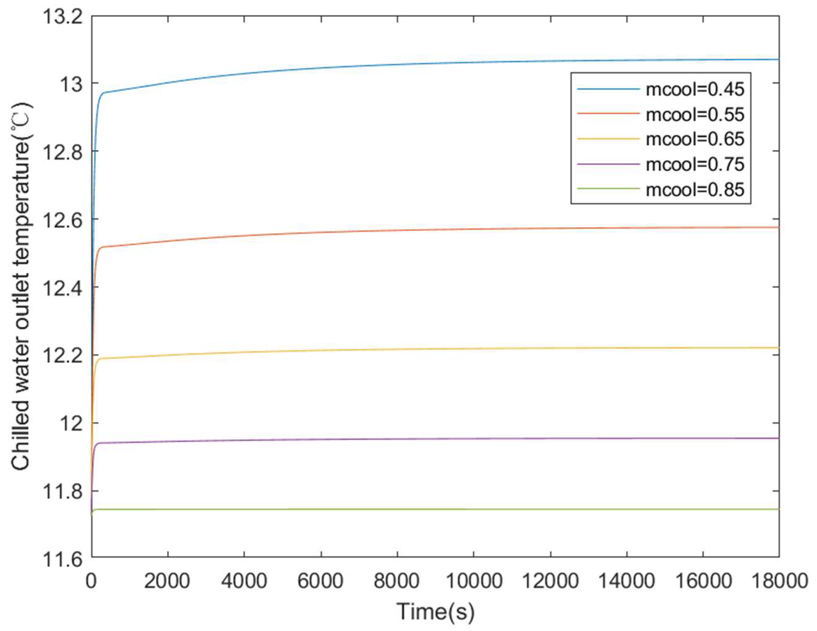
2.7. Influence of Cooling Water Flow Rate on Chilled Water Outlet Temperature

After setting the unit’s hot, cooling, and chilled water inlet temperatures at 95 °C, 32 °C, and 15 °C, respectively, the chilled water flow rate at 0.26 kg/s, and the solution pump frequency at 30 Hz, and maintaining the mass flow rate of hot water at 0.32 kg/s, simulations began with a cooling water mass flow rate of 0.65 kg/s. During the simulation, every 2000 s, the cooling water mass flow rate was adjusted up or down by 0.1 kg/s. The simulation duration was 18,000 s, and the results are shown in Figure 1.

In Figure 2, it can be observed that, under unchanged external conditions, the outlet temperature of chilled water from the unit decreases with increasing cooling water flow rate and increases with decreasing cooling water flow rate. This is because increasing the cooling water flow rate can lower the temperature of the lithium bromide solution in the absorber, enhance the solution’s moisture absorption capacity, accelerate the absorption rate of refrigerant water vapor, increase the evaporator load, and improve the unit’s cooling capacity.

Additionally, the figure shows that, immediately after each adjustment of the cooling water flow rate, the outlet temperature of chilled water from the unit changes rapidly for approximately 200 s, followed by a slower change over the next 1800 s. This phenomenon occurs because a sudden change in the cooling water flow rate directly affects the state of the solution in the absorber, leading to rapid changes in the low-pressure side pressure of the unit. During this time, the chilled water outlet temperature is primarily influenced by the absorber’s thermal inertia, resulting in rapid changes. As the unit continues to operate, changes in the state of the solution at the outlet of the absorber gradually affect the generator and the entire high-pressure side, causing changes in the state of refrigerant water at the condenser outlet, indirectly affecting the unit’s chilled water outlet temperature. This process involves three major thermal inertia stages, leading to relatively slow changes in the chilled water temperature.

Figure 3 depicts the curves of the unit’s chilled water outlet temperature under different cooling water flow rate conditions. The arrows in the figure indicate the mass flow rate of cooling water, ranging from 0.45 to 0.85 kg/s. It can be observed that the chilled water outlet temperature decreases with increasing cooling water flow rate, increasing when the latter decreases. Therefore, under unchanged conditions, increasing the cooling water flow rate can enhance the unit’s refrigeration capacity, while reducing the cooling water flow rate can decrease it.

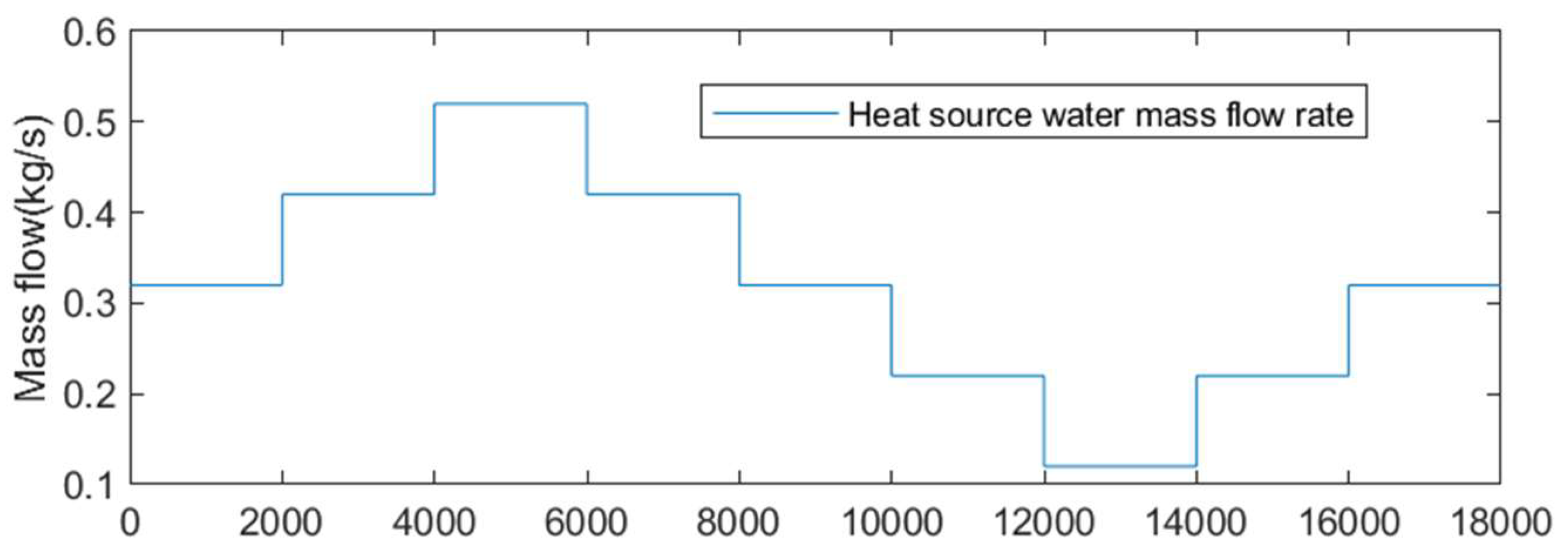
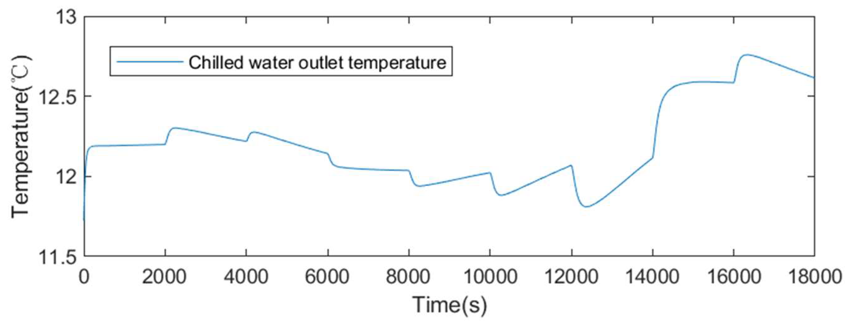
2.8. Influence of Heat Source Water Flow Rate on Chilled Water Outlet Temperature

After setting the heat source, cooling, and chilled water inlet temperatures to 95 °C, 32 °C, and 15 °C, respectively, the chilled water flow rate to 0.26 kg/s, and the solution pump frequency to 30 Hz and keeping the cooling water mass flow rate constant at 0.65 kg/s, simulations were initiated with a heat source water mass flow rate of 0.32 kg/s. During the simulation, the heat source water mass flow rate was adjusted up or down by 0.1 kg/s every 2000 s, and the results are shown in Figure 4.

From the figure, it is evident that, under unchanged conditions, the outlet temperature of chilled water from the unit decreases with increasing heat source water flow rate, increasing when the latter decreases. This is because increasing the heat source water flow rate raises the temperature and concentration of the lithium bromide solution at the generator outlet, thereby enhancing the solution’s ability to absorb refrigerant water vapor in the absorber and increasing the evaporator’s refrigeration capacity. Conversely, reducing the heat source water flow rate decreases the solution concentration at the generator outlet and reduces the absorption rate of the refrigerant water vapor in the lithium bromide solution in the absorber, thereby inhibiting the evaporator’s refrigeration capacity.

Similar to the situation with cooling water flow rate changes, due to the thermal inertia of various unit components, there is a brief overshoot transition phase after a step change in the heat source water flow rate. However, this transition is less pronounced compared to changes in the cooling water flow rate because changes in the generator state do not directly affect the evaporator state but indirectly affect the evaporator outlet temperature of chilled water through their impact on the absorber and condenser states.

The curves of the unit’s chilled water outlet temperature under different heat source water flow rate conditions are shown in Figure 5. The arrows indicate the mass flow rate of the heat source water, ranging from 0.12 to 0.52 kg/s. It can be observed that a higher heat source water flow rate results in a lower chilled water outlet temperature from the unit and a higher cooling capacity. Conversely, a lower heat source flow rate leads to a higher chilled water outlet temperature and a reduced cooling capacity of the unit. Additionally, as the heat source water flow rate increases, the ability to adjust the unit’s cooling capacity gradually diminishes. For instance, increasing the heat source water flow rate from 0.12 kg/s to 0.22 kg/s reduces the outlet temperature of chilled water from approximately 13.8 °C to approximately 12.92 °C, a cooling reduction of about 0.88 °C. In contrast, increasing the heat source water flow rate from 0.42 kg/s to 0.52 kg/s reduces the outlet temperature from approximately 12.3 °C to approximately 12.15 °C, a cooling reduction of only about 0.15 °C, which is approximately 17% of the reduction observed at lower flow rates. Thus, the capacity to adjust the unit load solely through heat source water flow rate modulation is limited.

3. Control Strategy

In absorption refrigeration systems, the selection of manipulated and controlled variables is crucial. Increasing the flow rates of heat sources or cooling water and adjusting their inlet temperatures can increase refrigeration capacity, within certain limits. However, such adjustments typically increase energy consumption and costs, thus impacting economic feasibility. Therefore, setting the inlet temperatures of the heat source and cooling water as external input parameters rather than manipulated variables is advisable. While the solution’s circulation rate is adjustable, it can lead to drastic changes in internal system states, posing safety risks. Consequently, a fixed-solution pump control program is designed to prevent arbitrary changes. The chilled water flow rate is related to the system load and treated as an external input.

The selection of the heat source and cooling water flow rates as manipulated variables, with the unit’s chilled water outlet temperature as the controlled variable, forms the basis of control system design in absorption refrigeration systems.

Modeling absorption refrigeration systems presents challenges in control system design. The foundation for most advanced control techniques relies on establishing mathematical models of the controlled systems. However, in practical industrial processes, it is often difficult to establish precise mathematical models, especially for nonlinear systems. Even when models of controlled systems are established, they are often greatly simplified and may not effectively describe the systems’ characteristics. Consequently, controllers developed based on these models may encounter issues when applied to actual systems. Therefore, the primary purpose of complex system modeling is often to study system characteristics.

To date, controllers for absorption refrigeration systems predominantly utilize PID (proportional–integral–derivative) control technology commonly used in engineering [34]. Its advantages lie in its simplicity and ease of implementation, without requiring a precise mathematical model of the controlled system. However, PID controllers suffer from drawbacks such as the need for parameter retuning when process conditions change, coupled adjustments of three tunable parameters, and inconvenience in achieving a satisfactory performance. For lithium bromide absorption refrigeration systems with strong nonlinearities, time-varying behavior, structural variations, and parameter uncertainties, PID controllers struggle to balance the conflicting demands between dynamic and static system characteristics, often leading to excessive overshoot, long settling times, and instability.

Model-free adaptive control (MFAC) is a data-driven nonlinear system control algorithm proposed by Professor Hou Zhongsheng. Its fundamental concept involves establishing dynamic linearized models equivalent to nonlinear systems at each operating point. A key feature is its independence from the mathematical model of the controlled object, enabling the computation of control quantities and estimates based solely on system input–output data [35]. MFAC does not require precise quantitative process knowledge, ensuring closed-loop stability with simple parameter tuning, broad applicability, and a degree of “self-decoupling” functionality [36], making it suitable for complex absorption refrigeration system control.

MFAC inherits research achievements from adaptive control in linear systems by dynamically linearizing nonlinear systems at each moment, thereby eliminating unmodeled dynamics and significantly enhancing control system robustness against disturbances or parameter variations. MFAC comprises the dynamic linearization of nonlinear systems, including compact-, partial-, and full-format models (CFDL, PFDL, and FFDL, respectively), each of them giving rise to derivative MFAC methods, alongside parameter estimation and control law design. This paper proposes an MFAC scheme for absorption refrigeration systems based on compact-format dynamic linearization.

3.1. Single-Loop Control of Absorption Refrigeration Systems

The predominant control method for absorption refrigeration systems involves a single-loop control structure in which the outlet temperature of chilled water from the unit serves as the controlled variable, with the heat source flow rate or inlet temperature as the manipulated variables. The control structure is illustrated in Figure 6.

The model of the absorption refrigeration system is typically represented as a general form of a single-input and single-output (SISO) nonlinear system model:

$$y\left(k+1\right)=f\left(y\left(k\right),y\left(k-1\right),\cdot \cdot \cdot ,y\left(k-n_y\right),u\left(k\right),u\left(k-1\right),\cdot \cdot \cdot ,u\left(k-n_u\right)\right)$$

(19)

Here, $u\left(k\right)$ represents the heat source water flow rate at time k; $y\left(k\right)$ denotes the outlet temperature of chilled water from the unit at time $k$; $n_y$ and $n_u$ represent the unknown order of the system, typically identified through model identification methods; and $f\left(\cdot \cdot \cdot \right)$ represents the unknown nonlinear function of the system.

Assumption 1. 

System (1) exhibits a feasible control input signal $y^{*}\left(k+1\right)$ that is bounded for a bounded desired output signal, under which the system output equals the desired output.

Assumption 2. 

The partial derivatives $f\left(\cdot \cdot \cdot \right)$ of the system with respect to the control input signal $u\left(k\right)$ are continuous.

Assumption 3. 

The system is a generalized Lipschitz system, meaning that, for any $k$, there exists a constant $\left|\Delta y\left(k+1\right)\right|\le b\left|\Delta u\left(k\right)\right|$ such that, for all $\Delta u\left(k\right)\ne 0$, $\Delta y\left(k+1\right)=y\left(k+1\right)-y\left(k\right)$ and $\Delta u\left(k\right)=u\left(k\right)-u\left(k-1\right)$, where $b$ is a function of the system.

Assumption 4. 

For any input $u\left(k\right)$, the system has continuous partial derivatives and satisfies the generalized Lipschitz condition, i.e., for any $k$, there exists a positive constant $L$ such that, for all, $\left|\Delta y\left(k+1\right)\right|\le L\left|\Delta u\left(k\right)\right|$.

Theorem 1. 

For a nonlinear system (1), if Assumptions 1–3 are satisfied, then there exists a time-varying parameter vector $\varphi \left(k\right)$ such that, for all $\Delta u\left(k\right)\ne 0$,

$$\Delta y\left(k+1\right)=\varphi \left(k\right)\Delta u\left(k\right)$$

(20)

System (1) can be replaced by the following dynamically linearized model based on the tight-format linearization method:

$$y\left(k+1\right)=y\left(k\right)+\varphi \left(k\right)\Delta u\left(k\right)$$

(21)

The vector $\left|\varphi \left(k\right)\right|\le b$ is based on the pseudo-partial derivative (PPD) of compact-format linearization, which is a time-varying parameter. It transforms a complex single-input single-output (SISO) nonlinear system into a time-varying linear system with a single parameter. If the sampling period and $\Delta u\left(k\right)$ are very small, $\varphi \left(k\right)$ can be considered a slowly time-varying parameter, and the relationship between $\varphi \left(k\right)$ and parameter $u\left(k\right)$ can be neglected. To meet the requirement of the rate of change of the control input signal $\Delta u\left(k\right)\ne 0$ and $\Delta u\left(k\right)$ being small, the following control input criterion function is introduced:

$$\min J\left(u\left(k\right)\right)={\left|y^{\ast }\left(k+1\right)-y\left(k+1\right)\right|}^2+\lambda {\left|u\left(k\right)-u\left(k-1\right)\right|}^2$$

(22)

By taking the derivative of both sides of the equation with respect to $u\left(k\right)$ and setting it to zero, the model-free control law for the SISO system is obtained as follows:

$$u\left(k\right)=u\left(k-1\right)+{\displaystyle \frac{\rho \varphi \left(k\right)}{\lambda +{\left|\varphi \left(k\right)\right|}^2}}\left[y^{\ast }\left(k+1\right)-y\left(k\right)\right]$$

(23)

wherein $\rho$ denotes the step size sequence and $\lambda$ represents the weight factor, which serves to constrain the magnitude of the input change $\Delta u\left(k\right)$, ensuring the reasonable substitution range of Equation (3) for Equation (1), indirectly limiting the variation of the pseudo-partial derivative and simultaneously avoiding the singularity caused by a zero denominator in Equation (5).

The term $\varphi \left(k\right)$ in Equation (5) is the unique unknown parameter. To prevent the estimated parameter value from changing too rapidly and avoid an excessively large linearization substitution range, the following parameter estimation criterion function is introduced:

$$\min J\left(\varphi \left(k\right)\right)={\left|y\left(k\right)-y\left(k-1\right)-\varphi \left(k\right)\Delta u\left(k-1\right)\right|}^2+\mu {\left|\varphi \left(k\right)-\widehat{\varphi }\left(k-1\right)\right|}^2$$

(24)

After a process of minimization, the algorithm for estimating the pseudo-partial derivative is derived as follows:

$$\widehat{\varphi }\left(k\right)=\widehat{\varphi }\left(k-1\right)+{\displaystyle \frac{\eta \Delta u\left(k-1\right)}{\mu +{\left|\Delta u\left(k-1\right)\right|}^2}}\left[\Delta y\left(k\right)-\widehat{\varphi }\left(k-1\right)\Delta u\left(k-1\right)\right]$$

(25)

$$\widehat{\varphi }\left(k\right)=\widehat{\varphi }\left(1\right), \left|\widehat{\varphi }\left(k\right)\right|\le \epsilon \mathrm{or} \Delta u\left(k-1\right)\le \epsilon$$

(26)

$\eta$ denotes the step size sequence; $\mu$ is a penalty factor related to the estimation of parameter changes, which constrains the range of linear substitution for the nonlinear system; $\epsilon$ is a sufficiently small, positive constant; $\widehat{\varphi }\left(k\right)$ represents the online estimate of the pseudo-partial derivative; and $\widehat{\varphi }\left(1\right)$ is the initial value of $\widehat{\varphi }\left(k\right)$.

Combining these elements, the model-free adaptive control law for the SISO system can be described as follows:

$$u\left(k\right)=u\left(k-1\right)+{\displaystyle \frac{\rho \widehat{\varphi }\left(k\right)}{\lambda +{\left|\widehat{\varphi }\left(k\right)\right|}^2}}\left[y^{\ast }\left(k+1\right)-y\left(k\right)\right]$$

(27)

Based on the model-free control law, a classic model-free control structure block diagram can be drawn, as shown in Figure 7. From the figure, it can be intuitively seen that the control law of the model-free adaptive control system is independent of the order and structure of the controlled system, relying solely on the system’s input and output data. Additionally, it has only one online adjustable controller parameter, the pseudo-partial derivative (PPD), which facilitates implementation.

Building on Equation (1), and considering the time-delay characteristics of the absorption refrigeration system, the system model can be further represented as the following SISO discrete-time system with a time-delay component:

$$y\left(k+1\right)=f\left(y\left(k\right),y\left(k-1\right),\cdot \cdot \cdot ,y\left(k-n_y\right),u\left(k\right),u\left(k-\tau \right),\cdot \cdot \cdot ,u\left(k-\tau -n_u\right)\right)$$

(28)

where $\tau$ represents the time-delay constant. To better accommodate the delayed system, a control input rate constraint term with a time delay is added to the control input criterion function in Equation (4). The revised input control criterion function is written as follows:

$$\begin{array}{cc}\hfill \min J\left(u\left(k\right)\right)& ={\left[y^{\ast }\left(k+1\right)-y\left(k+1\right)\right]}^2+\lambda {\left[u\left(k\right)-u\left(k-1\right)\right]}^2\hfill \\ & +\eta {\left[{\displaystyle \frac{u\left(k\right)-u\left(k-1-\tau \right)}{T}}\right]}^2\hfill \end{array}$$

(29)

$\lambda$ and $\eta$ are positive weighting factors. Taking the partial derivative of both sides of Equation (11) with respect to $u\left(k\right)$ and setting it to zero, the model-free control law for the delayed nonlinear system is obtained as follows:

$$\begin{array}{c}u\left(k\right)=u\left(k-1\right)+{\displaystyle \frac{\rho \widehat{\varphi }\left(k\right)}{\lambda +{\left|\widehat{\varphi }\left(k\right)\right|}^2+\frac{\eta }{T^2}}}\left[y^{\ast }\left(k+1\right)-y\left(k\right)\right]\\ +{\displaystyle \frac{\frac{\eta }{T^2}}{\lambda +{\left|\widehat{\varphi }\left(k\right)\right|}^2+\frac{\eta }{T^2}}}\left[u\left(k-1-\tau \right)-u\left(k-1\right)\right]\end{array}$$

(30)

$\rho \in \left(0,1\right)$ is the step-size sequence. $\widehat{\varphi }\left(k\right)$ is the online estimate of $\varphi \left(k\right)$, with the estimation criterion function provided as follows:

$$\begin{array}{c}\min J\left(\varphi \left(k\right)\right)={\left|y\left(k\right)-y\left(k-1\right)-\varphi \left(k\right)\Delta \left(k-1\right)\right|}^2\\ +\mu {\left|\varphi \left(k\right)-\varphi \left(k-1\right)\right|}^2\end{array}$$

(31)

Taking into account the influence of the time-delay characteristics on the controlled object, $u\left(k-1\right)-u\left(k-2-\tau \right)$ is used to replace $\Delta u\left(k-1\right)$ in Equation (13), and the estimation criterion function becomes the following:

$$\begin{array}{cc}\hfill \min J\left(\varphi \left(k\right)\right)& ={\left|y\left(k\right)-y\left(k-1\right)-\varphi \left(k\right)\left[\left(k-1\right)-\left(k-2-\tau \right)\right]\right|}^2\hfill \\ & +\mu {\left|\varphi \left(k\right)-\varphi \left(k-1\right)\right|}^2\hfill \end{array}$$

(32)

By differentiating both sides of Equation (14) with respect to $\varphi \left(k\right)$ and setting the result to zero, the pseudo-partial derivative parameter estimation algorithm for the time-delay model-free controller is obtained as follows:

$$\begin{array}{cc}\hfill \widehat{\varphi }\left(k\right)& =\widehat{\varphi }\left(k-1\right)+{\displaystyle \frac{\xi \left[u\left(k-1\right)-u\left(k-2-\tau \right)\right]}{\mu +{\left|u\left(k-1\right)-u\left(k-2-\tau \right)\right|}^2}}\hfill \\ & \times \left\{\Delta y\left(k\right)-\widehat{\varphi }\left(k-1\right)\left[u\left(k-1\right)-u\left(k-2-\tau \right)\right]\right\}\hfill \end{array}$$

(33)

$$\widehat{\varphi }\left(k\right)=\widehat{\varphi }\left(1\right), \left|\widehat{\varphi }\left(k\right)\right|\le \epsilon \mathrm{or} \Delta u\left(k-1\right)\le \epsilon$$

(34)

$\xi \in \left(0,1\right)$ is the step-size sequence, $\mu$ is the weight factor, and $\widehat{\varphi }\left(1\right)$ is the initial value of the pseudo-partial derivative estimation $\widehat{\varphi }\left(k\right)$. The block diagram of the model-free adaptive control system with delay is shown in Figure 8.

3.2. Double-Closed-Loop Energy Control for Absorption Refrigeration Systems

Although the single-loop control scheme for absorption refrigeration systems can meet the refrigeration load requirements, it maintains a constant cooling water flow rate, which can lead to the waste of both electricity and heat sources when the load is small, thereby reducing the system’s coefficient of performance (SCOP) and failing to achieve optimal system control.

To ensure efficient system operation while meeting the refrigeration load demands, the global optimization algorithm is introduced into the control of absorption refrigeration systems. This algorithm determines the optimal setpoints for the system to reach a stable state based on external operating conditions and load demands. An auxiliary controlled variable is added to the control system. Considering that the generator is directly connected to the heat source water and that some scholars have achieved system refrigeration capacity regulation using the generator temperature as a controlled variable, the generator temperature is selected as the additional controlled variable. The heat source water flow rate is used to control the generator temperature, while the cooling water flow rate controls the temperature of the chilled water outlet from the refrigeration unit. This allows the system to track the optimal setpoints. The double-closed-loop energy control strategy for the system is thus designed, as shown in Figure 9.

With the thermal source and cooling water flow rates as the operating variables and the chilled water outlet and generator temperatures as the controlled variables, an absorption refrigeration system can be considered a dual-input dual-output system. For the sake of generality, the absorption refrigeration system can be represented in the following unified form of a multi-input multi-output (MIMO) discrete-time nonlinear system with time delay:

$$y\left(k+1\right)=f\left(y\left(k\right),y\left(k-1\right),\dots ,y\left(k-n_y\right),u\left(k\right),u\left(k-\tau \right),\dots ,u\left(k-\tau -n_u\right)\right)$$

(35)

$u\left(k\right),y\left(k\right)\in R^m$ are the input and output vectors of the system, respectively; $f\left(\dots \right)$ is an unknown nonlinear function; $n_y,n_u$ represent the unknown order of the system; and $\tau$ is the time delay of the system.

For a discrete-time MIMO (multiple-input multiple-output) system (17) with delay that satisfies Assumption 4, the compact-format dynamic linearization model can be expressed as follows:

$$y\left(k+1\right)=y\left(k\right)+\mathit{\varphi }\left(k\right)\Delta u\left(k\right)$$

(36)

$$\mathit{\varphi }\left(k\right)=\left[\begin{array}{cccc}{\mathit{\varphi }}_1\left(k\right)& {\mathit{\varphi }}_2\left(k\right)& \dots & {\mathit{\varphi }}_m\left(k\right)\end{array}\right] \mathrm{and} \Vert \mathit{\varphi }\left(k\right)\Vert \le L, {\mathit{\varphi }}_i\left(k\right)={\left[\begin{array}{cccc}{\varphi }_{i1}& {\varphi }_{i2}& \dots & {\varphi }_{im}\end{array}\right]}^T,i=1,2,\dots ,m$$

Similar to the case of time-delayed SISO discrete-time systems, the model-free control law derivation for time-delayed MIMO systems employs the following criterion function:

$$\begin{array}{c}\min J\left(u\left(k\right)\right)={\left[y^{\ast }\left(k+1\right)-y\left(k+1\right)\right]}^2+\lambda {\Vert u\left(k\right)-u\left(k-1\right)\Vert }^2\\ +\eta {\Vert {\displaystyle \frac{u\left(k\right)-u\left(k-1-\tau \right)}{T}}\Vert }^2\end{array}$$

(37)

$u\left(k-1-\tau \right)=\left[u_1\left(k-1-{\tau }_1\right),\dots ,u_m\left(k-1-{\tau }_m\right)\right]$, and taking partial derivatives of $u\left(k\right)$ on both sides of the equation yields the following:

$$\begin{array}{cc}\hfill \min {\displaystyle \frac{\partial J\left(u\left(k\right)\right)}{\partial u\left(k\right)}}& =-2{\mathit{\varphi }}^T\left(k\right)\left[y^{\ast }\left(k+1\right)-y\left(k\right)-\mathit{\varphi }\left(k\right)\Delta u\left(k\right)\right]\hfill \\ & +2\lambda \left[u\left(k\right)-u\left(k-1\right)\right]+{\displaystyle \frac{2\eta }{T^2}}\left[u\left(k-1-\tau \right)-u\left(k\right)\right]\hfill \end{array}$$

(38)

Setting this equal to zero produces the model-free control law for MIMO systems:

$$\begin{array}{c}u\left(k\right)=u\left(k-1\right)+{\displaystyle \frac{\rho {\widehat{\mathit{\varphi }}}^T\left(k\right)}{\lambda +\frac{\eta }{T^2}+{\Vert \widehat{\mathit{\varphi }}\left(k\right)\Vert }^2}}\left[y^{\ast }\left(k+1\right)-y\left(k\right)\right]\\ +{\displaystyle \frac{\frac{\eta }{T^2}}{\lambda +\frac{\eta }{T^2}+{\Vert \widehat{\mathit{\varphi }}\left(k\right)\Vert }^2}}\left[u\left(k-1\right)-u\left(k-1-\tau \right)\right]\end{array}$$

(39)

where $\widehat{\mathit{\varphi }}\left(k\right)$ is the estimated pseudo-derivative vector of $\mathit{\varphi }\left(k\right)$, the sole unknown parameter in the model-free control law. Similar to SISO time-delay systems, the criterion function for estimating the pseudo-derivative vector in model-free controllers for MIMO time-delay systems is expressed as follows:

$$\begin{array}{cc}\hfill \min J\left(\mathit{\varphi }\left(k\right)\right)& ={\left|y\left(k\right)-y\left(k-1\right)-\mathit{\varphi }\left(k\right)\left[u\left(k-1\right)-u\left(k-2-\tau \right)\right]\right|}^2\hfill \\ & +\mu {\Vert \mathit{\varphi }\left(k\right)-\mathit{\varphi }\left(k-1\right)\Vert }^2\hfill \end{array}$$

(40)

Using partial derivatives of $\mathit{\varphi }\left(k\right)$ on both sides of Equation (22) produces the following equation:

$$\begin{array}{cc}\hfill \min {\displaystyle \frac{\partial J\left(\mathit{\varphi }\left(k\right)\right)}{\partial \mathit{\varphi }\left(k\right)}}& =-2\left[y\left(k\right)-y\left(k-1\right)\right]\left[u\left(k-1\right)-u\left(k-2-\tau \right)\right]\hfill \\ & +2\mathit{\varphi }\left(k\right){\Vert u\left(k-1\right)-u\left(k-2-\tau \right)\Vert }^2+2\mu \left[\mathit{\varphi }\left(k\right)-\mathit{\varphi }\left(k-1\right)\right]\hfill \end{array}$$

(41)

Setting Equation (23) equal to zero produces the pseudo-derivative estimation algorithm for MIMO delayed model-free controllers:

$$\begin{array}{cc}\hfill \widehat{\mathit{\varphi }}\left(k\right)& =\widehat{\mathit{\varphi }}\left(k-1\right)+{\displaystyle \frac{\xi \left\{\Delta y\left(k\right)-\widehat{\mathit{\varphi }}\left(k-1\right)\left[u\left(k-1\right)-u\left(k-2-\tau \right)\right]\right\}}{\mu +{\Vert u\left(k-1\right)-u\left(k-2-\tau \right)\Vert }^2}}\hfill \\ & \times {\left[u\left(k-1\right)-u\left(k-2-\tau \right)\right]}^T\hfill \end{array}$$

(42)

where $\lambda >0$, $\eta >0$, and $\mu >0$ are the weighting coefficients, and $\rho \in \left(0,1\right]$ and $\xi \in \left(0,2\right]$ are the step sequences. It is evident that the model-free control algorithm for MIMO systems is generalizable without a loss of generality. The structural control diagram can be represented by Figure 9. If the number of input variables is one, the controller structure is identical to that of SISO time-delay systems. Further, if the time-delay constant $\tau$ is equal to zero, it becomes the classical model-free control algorithm for single-input single-output systems.

The authors of [25] demonstrated the convergence of the classical model-free control algorithm. Meanwhile, Jin Shangtai et al. [26] proposed an improved model-free control algorithm for SISO delayed systems and proved its convergence. This can be directly extended to prove the convergence of the model-free control algorithm for MIMO delayed systems, although the proof is omitted in this paper.

4. Simulation Experiment and Results

This study applies model-free control algorithms to both the single- and dual-loop control of absorption refrigeration systems, validating the effectiveness of the control strategies through simulations and experiments.

4.1. Simulation Study of Single-Loop Energy-Saving Control

Building upon the dynamic model of a hot-water single-effect lithium bromide absorption refrigeration system established in a previous work, where the unit’s thermal source water flow rate serves as the operating variable and the chilled water outlet temperature as the controlled variable, a simulation model for the single-loop control of this system, as depicted in Figure 6, was constructed. The control objective was to maintain a chilled water outlet temperature of 12 °C. PID control, classical model-free adaptive control (MFAC), and time-delayed MFAC were separately applied to simulate the single-loop control of the absorption refrigeration system.

Table 2. Absorption refrigeration system’s closed-loop control simulation with external input parameters.

Heat Source Water Inlet Temperature ${\mathit{T}}_{\mathbf{11}}$	Cooling Water Inlet Temperature ${\mathit{T}}_{\mathbf{13}}$	Chilled Water Inlet Temperature ${\mathit{T}}_{\mathbf{16}}$	Cooling Water Flow Rate ${\dot{\mathit{m}}}_{\mathbf{clw}}$	Chilled Water Flow Rate ${\dot{\mathit{m}}}_{\mathbf{17}}$	Solution Pump Frequency $\mathit{f}$
95 °C	30 °C	15 °C	0.65 kg/s	0.26 kg/s	30 Hz

presents the various experimental parameters.

The unit’s thermal source, cooling, and chilled water inlet temperatures were set to 95 °C, 30 °C, and 15 °C, respectively; the cooling and chilled water flow rates were 0.65 kg/s and 0.26 kg/s; and the solution pump frequency was 30 Hz.

The setpoint for the unit’s chilled water outlet temperature was 12 °C. The simulation duration was 3000 s. The PID controller parameters were $k_{\mathrm{p}}=0.2$, $k_{\mathrm{i}}=0.05$, and $k_{\mathrm{d}}=0$; the classical model-free controller parameters were $\eta =1$, $\rho =1$, $\mu =1.2$, $\lambda =0.1$, and $\widehat{\varphi }\left(1\right)=-1$; and the time-delayed model-free controller parameters were $\eta =1$, $\rho =1$, $\mu =1.2$, $\lambda =0.1$, and $\widehat{\varphi }\left(1\right)=-1$.

According to Figure 10, all three control methods can stabilize the system. However, under PID control, the system exhibits significant overshoot and a longer settling time. In contrast, both the time-delayed MFAC and classical MFAC methods show similar control effects, with shorter settling times and minimal overshoot.

4.2. Simulation Study of Dual-Loop Energy-Saving Control

Using the thermal source and cooling water flow rates of the absorption refrigeration unit as the control variables and the generator and chilled water outlet temperatures as the controlled variables, a dual-loop control simulation model for the system was constructed, as shown in Figure 9. Initially, based on the given external input parameters and the target chilled water outlet temperature, the target evaporating temperature was calculated to be 11.45 °C. Subsequently, using a setpoint optimization algorithm, the optimal steady-state setpoints for the unit were determined: a condensing temperature of 36.28 °C, a weak solution concentration of 53.9%, and a solution circulation ratio of eight. Finally, based on the steady-state model of the unit, the optimal generator temperature was calculated to be 85 °C.

Since the thermal source water came into direct contact with the generator and the time constant of the latter’s temperature delay was small and negligible, there was no need to use a time-delayed model-free controller. Therefore, the dual-loop control of the absorption refrigeration system was simulated using the following controller configurations.

Controller 1. 

PID controllers were employed for the generator and chilled water outlet temperatures, respectively. The parameters for the PID controller in the generator temperature loop were $k_{\mathrm{p}}=1$, $k_{\mathrm{i}}=1$, and $k_{\mathrm{d}}=0$, while those for the chilled water outlet temperature loop were $k_{\mathrm{p}}=-1$, $k_{\mathrm{i}}=-1$, and $k_{\mathrm{d}}=0$.

Controller 2. 

The generator and chilled water outlet temperatures were controlled using classical model-free adaptive controllers (MFACs) in a single-input single-output (SISO) configuration. The parameters for the classical MFAC in the generator temperature loop were $\eta =1$, $\rho =1$, $\mu =1$, $\lambda =10$, and $\widehat{\varphi }\left(1\right)=1$, while those for the chilled water outlet temperature loop were$\eta =1$, $\rho =1$, $\mu =1$, $\lambda =0.1$, and $\widehat{\varphi }\left(1\right)=-1$.

Controller 3. 

The generator temperature was controlled using classical single-input single-output (SISO) model-free adaptive control (MFAC), while the chilled water outlet temperature was controlled using a SISO model-free controller with time delay. The MFAC parameters for the generator temperature loop were $\eta =1$, $\rho =1$, $\mu =1$, $\lambda =10$, and $\widehat{\varphi }\left(1\right)=1$, while the MFAC parameters with time delay for the chilled water outlet temperature loop were $\eta =1$, $\rho =1$, $\mu =1$, $\lambda =5$, and $\widehat{\varphi }\left(1\right)=-1$.

Controller 4. 

A multiple-input multiple-output (MIMO) model-free controller with time delay was employed, with the following parameters: $\eta =1$, $\rho =1$, $\mu =1.2$, $\lambda =1$, and$\widehat{\varphi }\left(1\right)=\left[\begin{array}{cc}1& 0.1\\ 0.1& -1\end{array}\right]$.

The setpoint for the chilled water outlet temperature was 12 °C, and the generator temperature was set to the optimized target value of 85 °C. The simulation duration was 3000 s. To validate the disturbance rejection capability of the controller, a step disturbance with an amplitude of 0.2 °C was applied to the chilled water outlet temperature at 1500 s. The simulation results of the double-closed-loop energy control under the configurations of the four sets of controllers are shown in Figure 11 and Figure 12.

The figures indicate that, under the configurations of the four controllers, the absorption refrigeration systems can all reach a stable state. The PID controller exhibits a faster adjustment speed and achieves the best control effects. The control effects of the SISO classical MFAC and the SISO MFAC with time delay are essentially consistent, with the curves nearly overlapping. The MIMO model-free controller demonstrates the least effective control performance, with significant overshoot and a longer adjustment time but fewer parameters. When the chilled water outlet temperature is subjected to a disturbance, the cooling water flow rate, using the PID, undergoes severe oscillations, which can easily impact the cooling water pump. In contrast, the cooling water flow rate changes more smoothly with the model-free controller. The disturbance to the chilled water outlet temperature barely affects the unit’s generator temperature.

To evaluate the energy-saving effects of dual-loop energy-efficient control in absorption refrigeration systems, the parameters were compared under the following identical load conditions after achieving stability with single-loop and dual-loop energy-efficient control: chilled, cooling, and heat source water inlet temperatures of 15 °C, 32 °C, and 95 °C, respectively, a chilled water outlet temperature of 12 °C, and a chilled water flow rate of 0.26 kg/s. With a refrigeration capacity of 3.276 kW for both single-loop and dual-loop control strategies, heat consumption under the dual-loop control strategy was reduced by approximately 20% compared to the single-loop control, totaling 7.847 kW, and the electricity consumption decreased by about 10%, totaling 0.615 kW. The unit’s COP increased by 16.6%, to a total of 0.418, and the system’s overall SCOP improved by approximately 19.3%, to a value of 0.387, demonstrating the effectiveness of the dual-loop energy-efficient control scheme.

4.3. Experimental Study of the Model-Free Control of Absorption Refrigeration Systems

Although the effectiveness of the control strategies was demonstrated through simulation, various factors such as external parameters and system loads, may vary during actual system operation, making the system susceptible to disturbances which can significantly impact performance and stability. To validate the practical performance of the control method, a MIMO lag-free model-free control algorithm was applied to an experimental platform of a hot-water single-effect lithium bromide absorption refrigeration system. The system’s heat source water was supplied through a solar water heater and a hot water boiler to maintain a constant temperature, while the chilled water tank served as the system load. An electric heater in the tank balanced the system’s cooling capacity, ensuring a stable return water temperature for the refrigeration unit and minimizing unnecessary disturbances.

During the experiment, the chilled water flow rate was maintained at approximately 0.22 kg/s, with the supply water temperature from the refrigeration unit kept at 13 °C. The heat source water temperature was kept above 80 °C, and the cooling water temperature did not exceed 30 °C. Due to experimental constraints, slight fluctuations were observed in both the heat source and cooling water temperatures.

Experimental curves of the unit’s peripheral water return temperature and flow rate are shown in Figure 13 and Figure 14, respectively. As depicted in the figures, the chilled water supply temperature remains stable, at approximately 13 °C, under the action of the electric heater. Initially set at 11 °C, the setpoint of the chilled water outlet temperature stabilizes in the system; at 3000 s, it is step-adjusted to 10.1 °C and, at 5000 s and 7500 s, to 11.5 °C and 10.5 °C, respectively. Under the influence of the controller, the cooling water flow rate varies significantly with changes in the setpoint of the chilled water outlet temperature, while the heat source water flow rate remains relatively unchanged within the error range, consistent with the simulation results, verifying the effectiveness of the control method.

5. Conclusions

Absorption refrigeration systems, as important low-temperature thermal energy utilization devices, are widely employed in air conditioning and heat pumps, among other things, due to their advantages of having a simple structure and providing stable operation and low amounts of noise. However, due to their unique working principles, absorption refrigeration systems exhibit various dynamic characteristics, posing challenges in the design and implementation of control strategies. The following research results are based on the absorption refrigeration systems in this article:

• Based on the dynamic model of absorption refrigeration systems, an open-loop response characteristic analysis was conducted, identifying the control structure of these systems with the heat source and cooling water flow rates as the operating variables.
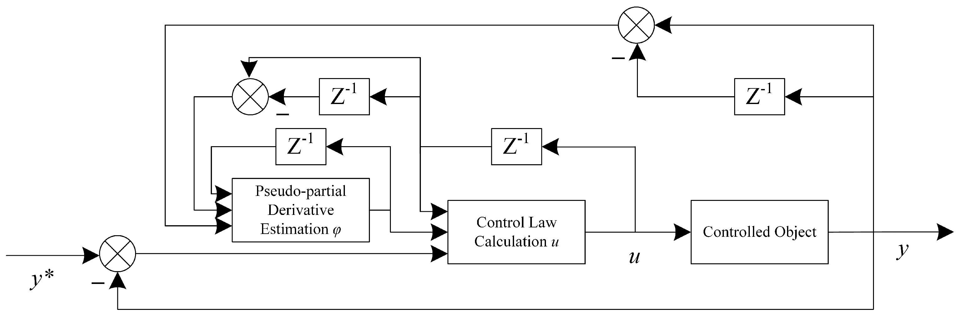
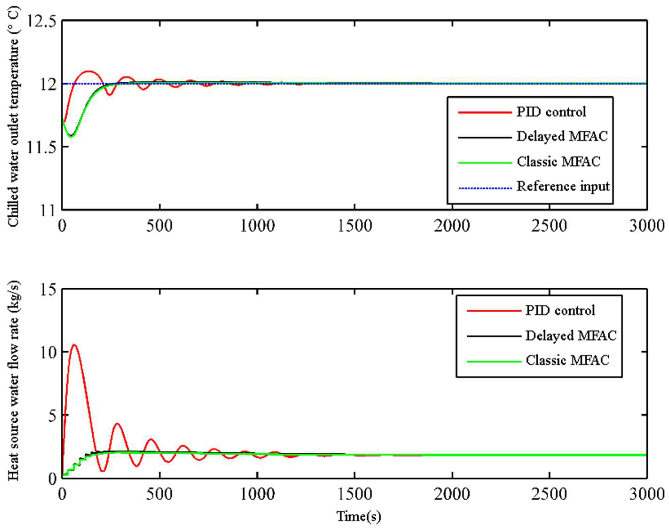
• Considering the complexity and modeling difficulties of absorption refrigeration system mechanisms, advanced control algorithms highly dependent on models cannot be applied. PID-like controllers, although commonly used, also struggle to achieve satisfactory control effects for multivariable, strongly coupled, and highly time-delayed and nonlinear absorption refrigeration systems. Model-free control algorithms, which do not require quantitative knowledge of the controlled object but rely solely on input–output data, exhibit good robustness. Therefore, a model-free control algorithm was selected for the control strategy design of absorption refrigeration systems.
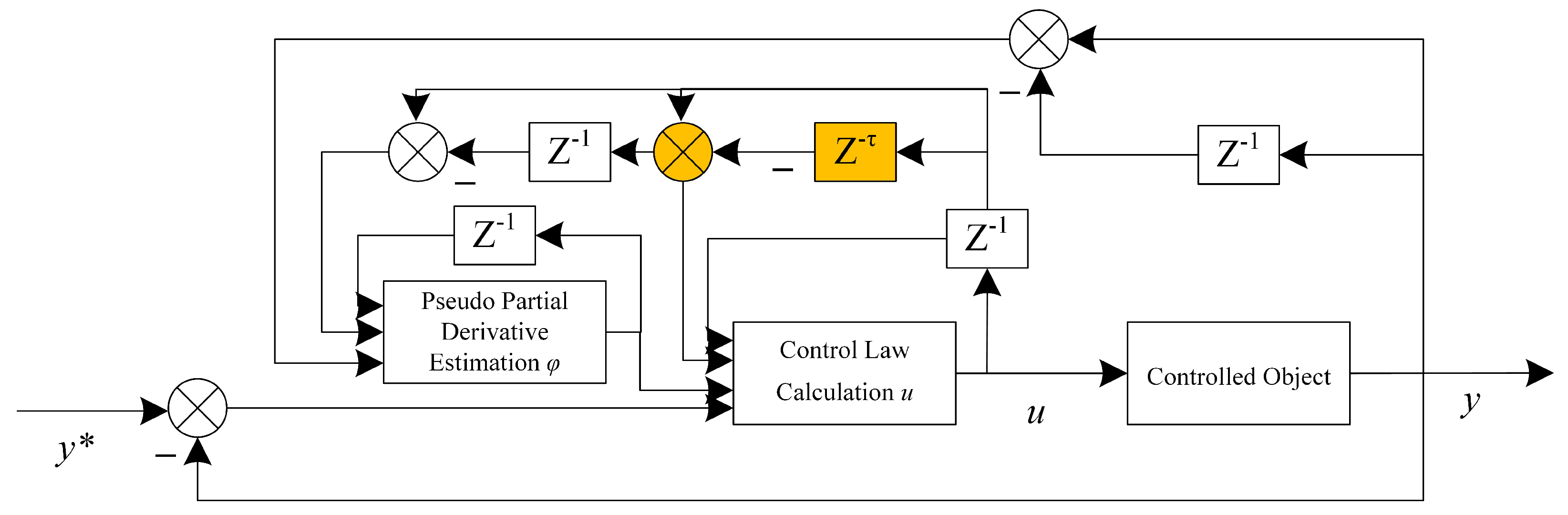
• Addressing the large time-delay characteristics of absorption refrigeration systems, a model-free control algorithm with time delay was derived based on classical model-free controllers.
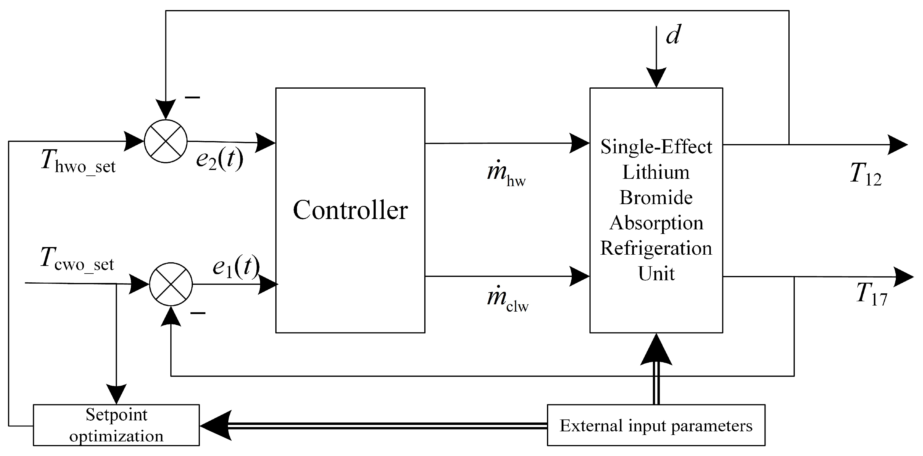
• Recognizing that single-loop control can only ensure the cooling capacity of the unit without guaranteeing its energy efficiency, an energy-saving dual-loop control scheme for absorption refrigeration systems was proposed based on setpoint ensemble optimization. A model-free MIMO control algorithm with time delay was derived accordingly.
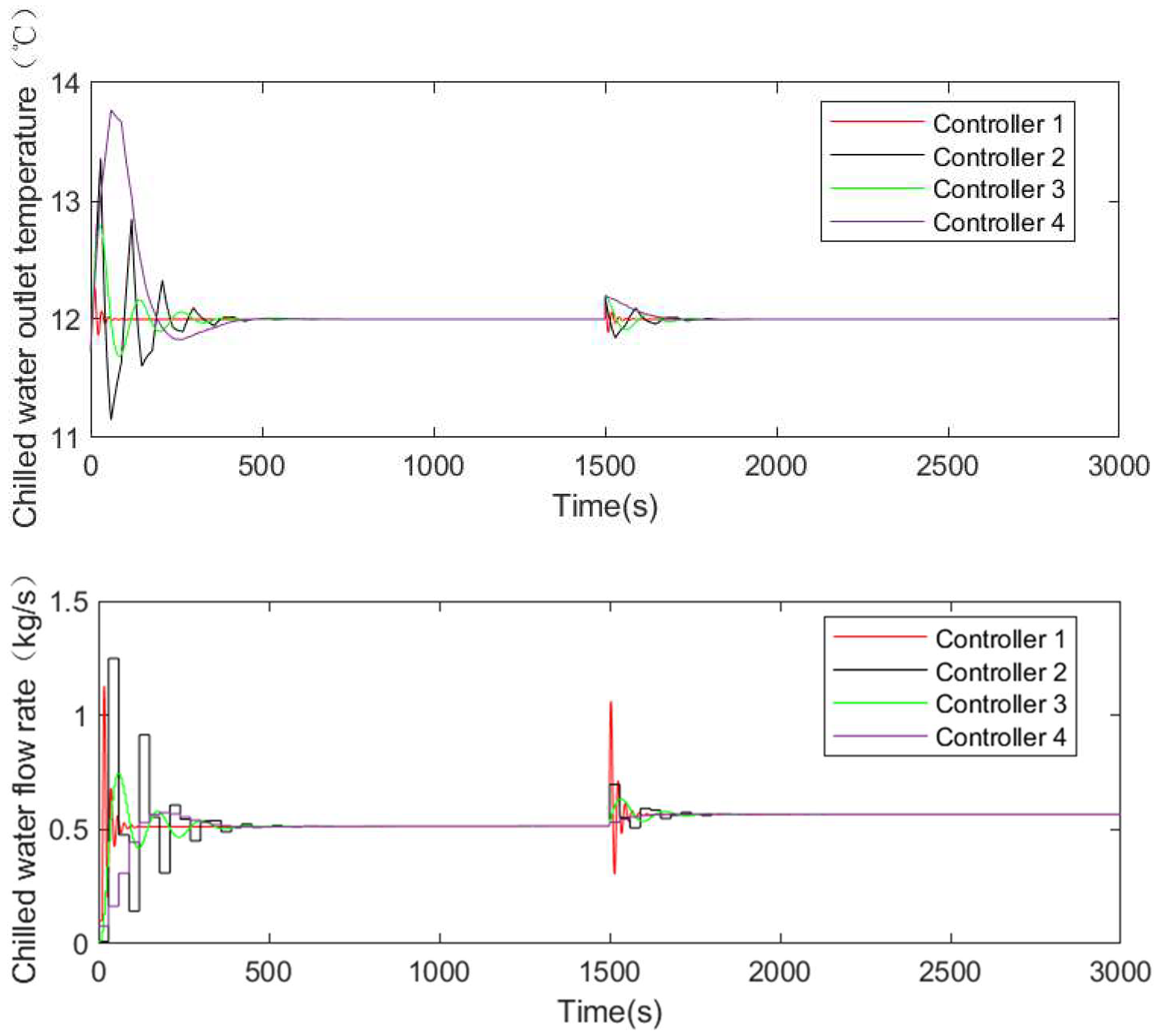
• Applying the model-free control algorithm to absorption refrigeration system control, simulations were conducted on single- and dual-loop energy-saving control strategies. The heat consumption was cut by approximately 20%, from 3.276 kW to 2.621 kW, under the dual-loop control strategy, which saved 0.655 kW compared to the other approach. Similarly, electricity consumption was reduced by about 10%, from 0.683 kW to 0.615 kW. These changes resulted in a 16.6% boost in the unit’s COP, from 0.360 to 0.418, and an overall improvement in the system’s SCOP of approximately 19.3%, from 0.330 to 0.387, showcasing the efficacy of the dual-loop energy-efficient control scheme.

References

1. Al-Sulaiman, F.A. Performance assessment of a solar powered ammonia–water absorption refrigeration system with storage units. Energy Convers. Manag. 2016, 126, 316–328. [Google Scholar]
2. Determan, M.D.; Garimella, S. Design, fabrication, and experimental demonstration of a microscale monolithic modular absorption heat pump. Appl. Therm. Eng. 2012, 47, 119–125. [Google Scholar] [CrossRef]
3. Verma, A.; Kaushık, S.C.; Tyagı, S.K. Performance enhancement of absorption refrigeration systems: An overview. J. Therm. Eng. 2023, 9, 1100–1113. [Google Scholar] [CrossRef]
4. Modi, B.; Mudgal, A.; Raja, B.D.; Patel, V. Low grade thermal energy driven-small scale absorption refrigeration system (SSARS): Design, fabrication and cost estimation. Sustain. Energy Technol. Assess. 2022, 50, 101787. [Google Scholar] [CrossRef]
5. Ahmad, T.; Azhar; Sinha, M.; Meraj; Mahbubul, I.M.; Ahmad, A. Energy analysis of lithium bromide-water and lithium chloride-water based single effect vapour absorption refrigeration system: A comparison study. Clean. Eng. Technol. 2022, 7, 100432. [Google Scholar] [CrossRef]
6. Chun, A.; Donatelli, J.L.M.; Santos, J.J.C.S.; Zabeu, C.B.; Carvalho, M. Superstructure optimization of absorption chillers integrated with a large internal combustion engine for waste heat recovery and repowering applications: Thermodynamic and economic assessments. Energy 2023, 263, 125970. [Google Scholar] [CrossRef]
7. Ham, J.; Yong, J.; Kwon, O.; Bae, K.; Cho, H. Experimental investigation on heat transfer and pressure drop of brazed plate heat exchanger using LiBr solution. Appl. Therm. Eng. 2023, 225, 120161. [Google Scholar] [CrossRef]
8. Zendehnam, A.; Pourfayaz, F. Sensitivity analysis of avoidable and unavoidable exergy destructions in a parallel double-effect LiBr–water absorption cooling system. Energy Sci. Eng. 2023, 11, 527–546. [Google Scholar] [CrossRef]
9. Vega, M.; Venegas, M.; García-Hernando, N. Modeling and performance analysis of an absorption chiller with a microchannel membrane-based absorber using LiBr-H2O, LiCl-H2O, and LiNO3-NH3. Int. J. Energy Res. 2018, 42, 3544–3558. [Google Scholar] [CrossRef]
10. Amaris, C.; Bourouis, M.; Vallès, M.; Salavera, D.; Coronas, A. Thermophysical properties and heat and mass transfer of new working fluids in plate heat exchangers for absorption refrigeration systems. Heat Transf. Eng. 2015, 36, 388–395. [Google Scholar] [CrossRef]
11. Didion, D.; Radermacher, R. Part-load performance characteristics of residential absorption chillers and heat pump. Int. J. Refrig. 1984, 7, 393–398. [Google Scholar] [CrossRef]
12. Alvares, S.G.; Trepp, C. Simulation of a solar driven aqua-ammonia absorption refrigeration system Part 1: Mathematical description and system optimization. Int. J. Refrig. 1987, 10, 40–48. [Google Scholar] [CrossRef]
13. Chen, L.; Zheng, T.; Sun, F.; Wu, C. Irreversible four-temperature-level absorption refrigerator. Solar Energy 2006, 80, 347–360. [Google Scholar] [CrossRef]
14. Cézar, K.L.; Caldas, A.G.A.; Caldas, A.M.A.; Cordeiro, M.C.L.; Dos Santos, C.A.C.; Ochoa, A.A.V.; Michima, P.S.A. Development of a novel flow control system with arduino microcontroller embedded in double effect absorption chillers using the LiBr/H2O pair. Int. J. Refrig. 2020, 111, 124–135. [Google Scholar] [CrossRef]
15. Staudt, S.; Unterberger, V.; Muschick, D.; Gölles, M.; Horn, M.; Wernhart, M.; Rieberer, R. MIMO state feedback control for redundantly-actuated LiBr/H2O absorption heat pumping devices and experimental validation. Control Eng. Pract. 2023, 140, 105661. [Google Scholar] [CrossRef]
16. Labus, J.; Hernández, J.; Bruno, J.; Coronas, A. Inverse neural network based control strategy for absorption chillers. Renew. Energy 2012, 39, 471–482. [Google Scholar] [CrossRef]
17. Alcântara, S.C.S.; Ochoa, A.A.V.; da Costa, J.Â.P.; de Menezes, F.D.; Leite, G.D.N.P.; Michima, P.S.A.; da Silva Marques, A. Development of a method for predicting the transient behavior of an absorption chiller using artificial intelligence methods. Appl. Therm. Eng. 2023, 231, 120978. [Google Scholar] [CrossRef]
18. Tang, C.; Li, N.; Bao, L. Predictive Control Modeling of Regional Cooling Systems Incorporating Ice Storage Technology. Buildings 2024, 14, 2488. [Google Scholar] [CrossRef]
19. Homod, R.Z.; Mohammed, H.I.; Ben Hamida, M.B.; Albahri, A.; Alhasnawi, B.N.; Albahri, O.; Alamoodi, A.; Mahdi, J.M.; Albadr, M.A.A.; Yaseen, Z.M. Optimal shifting of peak load in smart buildings using multiagent deep clustering reinforcement learning in multi-tank chilled water systems. J. Energy Storage 2024, 92, 112140. [Google Scholar] [CrossRef]
20. Faruque, W.; Khan, Y.; Nabil, M.H.; Ehsan, M.M. Parametric analysis and optimization of a novel cascade compression-absorption refrigeration system integrated with a flash tank and a reheater. Results Eng. 2023, 17, 101008. [Google Scholar] [CrossRef]
21. Altiokka, A.B.G.; Arslan, O. Design and optimization of absorption cooling system operating under low solar radiation for residential use. J. Build. Eng. 2023, 73, 106697. [Google Scholar] [CrossRef]
22. Sharifi, S.; Heravi, F.N.; Shirmohammadi, R.; Ghasempour, R.; Petrakopoulou, F.; Romeo, L. Comprehensive thermodynamic and operational optimization of a solar-assisted LiBr/water absorption refrigeration system. Energy Rep. 2020, 6, 2309–2323. [Google Scholar] [CrossRef]
23. Mohammadi, K.; Jiang, Y.; Borjian, S.; Powell, K. Thermo-economic assessment and optimization of a hybrid triple effect absorption chiller and compressor. Sustain. Energy Technol. Assess. 2020, 38, 100652. [Google Scholar] [CrossRef]
24. Marcos, J.D.; Izquierdo, M.; Palacios, E. New method for COP optimization in water- and air-cooled single and double effect LiBr–water absorption machines. Int. J. Refrig. 2011, 34, 1348–1359. [Google Scholar] [CrossRef]
25. Der, O.; Alqahtani, A.A.; Marengo, M.; Bertola, V. Characterization of polypropylene pulsating heat stripes: Effects of orientation, heat transfer fluid, and loop geometry. Appl. Therm. Eng. 2021, 184, 116304. [Google Scholar] [CrossRef]
26. Nikolayev, V.S. Physical principles and state-of-the-art of modeling of the pulsating heat pipe: A review. Appl. Therm. Eng. 2021, 195, 117111. [Google Scholar] [CrossRef]
27. Srikhirin, P.; Aphornratana, S.; Chungpaibulpatana, S. A review of absorption refrigeration technologies. Renew. Sustain. Energy Rev. 2001, 5, 343–372. [Google Scholar] [CrossRef]
28. Mendiburu, A.Z.; Roberts, J.J.; Rodrigues, L.J.; Verma, S.K. Thermodynamic modelling for absorption refrigeration cycles powered by solar energy and a case study for Porto Alegre, Brazil. Energy 2023, 266, 126457. [Google Scholar] [CrossRef]
29. Kaushik, S.C.; Arora, A. Energy and exergy analysis of single effect and series flow double effect water–lithium bromide absorption refrigeration systems. Int. J. Refrig. 2009, 32, 1247–1258. [Google Scholar] [CrossRef]
30. Bouaziz, N.; Lounissi, D. Energy and exergy investigation of a novel double effect hybrid absorption refrigeration system for solar cooling. Int. J. Hydrogen Energy 2015, 40, 13849–13856. [Google Scholar] [CrossRef]
31. Cui, P.; Yu, M.; Liu, Z.; Zhu, Z.; Yang, S. Energy, exergy, and economic (3E) analyses and multi-objective optimization of a cascade absorption refrigeration system for low-grade waste heat recovery. Energy Convers. Manag. 2019, 184, 249–261. [Google Scholar] [CrossRef]
32. Talbi, M.M.; Agnew, B. Exergy analysis: An absorption refrigerator using lithium bromide and water as the working fluids. Appl. Therm. Eng. 2000, 20, 619–630. [Google Scholar] [CrossRef]
33. Wen, H.; Wu, A.; Liu, Z.; Shang, Y. A state-space model for dynamic simulation of a single-effect LiBr/H2O absorption chiller. IEEE Access 2019, 7, 57251–57258. [Google Scholar] [CrossRef]
34. Rêgo, A.; Hanriot, S.; Oliveira, A.; Brito, P.; Rêgo, T. Automotive exhaust gas flow control for an ammonia–water absorption refrigeration system. Appl. Therm. Eng. 2014, 64, 101–107. [Google Scholar] [CrossRef]
35. Zhonsheng, H.; Jin, S. Model Free Adaptive Control Theory and Application; CRC Press: Boca Raton, FL, USA, 2014. [Google Scholar]
36. Jin, S.; Hou, Z. An improved model-free adaptive control for a class of nonlinear large-lag systems. Control Theory Appl. 2008, 25, 623–626. [Google Scholar]
Figure 1. Absorption refrigerating system. The blue arrow represents the heat release stage of the system, and the red arrow represents the heat absorption stage.
Energies 17 04658 g001
Figure 2. The impact of changes in the cooling water flow rate on the outlet temperature of chilled water.
Energies 17 04658 g002
Figure 3. Temperature curve of the unit’s chilled water outlet under different cooling water flow rates.
Energies 17 04658 g003
Figure 4. The influence of changes in the heat source water flow rate on the chilled water outlet temperature.
Energies 17 04658 g004aEnergies 17 04658 g004b
Figure 5. Temperature curve of the unit’s chilled water outlet under different heat source water flow rates.
Energies 17 04658 g005
Figure 6. Single-loop control structure diagram of an absorption refrigeration system.
Energies 17 04658 g006
Figure 7. Classic model-free control structure diagram.
Energies 17 04658 g007
Figure 8. Block diagram of model-free control structure with time delay.
Energies 17 04658 g008
Figure 9. Double-loop energy-saving control diagram of a single-effect lithium bromide absorption refrigeration system.
Energies 17 04658 g009
Figure 10. Single-loop control simulation of an absorption refrigeration system.
Energies 17 04658 g010
Figure 11. Double-closed-loop energy-saving control simulation of an absorption refrigeration system for chilled water outlet temperature control.
Energies 17 04658 g011
Figure 12. Double-closed-loop energy-saving control simulation of generator temperature control for an absorption refrigeration system.
Energies 17 04658 g012
Figure 13. Experimental curve of the water supply and return temperature around the unit.
Energies 17 04658 g013
Figure 14. Peripheral water supply flow curve of the unit.
Energies 17 04658 g014