
Methods for the Viscous Loss Calculation and Thermal Analysis of Oil-Filled Motors: A Review

 ,
,
Abstract
1. Introduction
2. Advancements in the Study of Viscous Loss
2.1. Methods for Calculating Viscous Loss

| Authors | Empirical Equations | Range | |
|---|---|---|---|
| Wendt [24] | (2) | 400 < ReG < 104 | |
| (3) | 104 < ReG < 105 | ||
| Yamada [25] | (4) | ||
| Bilgen and Boulos [26] | (5) | 500 < ReG < 104 | |
| (6) | ReG > 104 | ||
| Nakabayashi [27] | (7) | Ta < 1700 | |
| (8) | 1700 < Ta < 104 | ||
| (9) | Ta > 104 |
- Mass conservation: Continuity equation:
- Momentum conservation: Navier–Stokes equation:
- Energy conservation: Heat equation:
2.2. Factors Affecting Viscous Loss
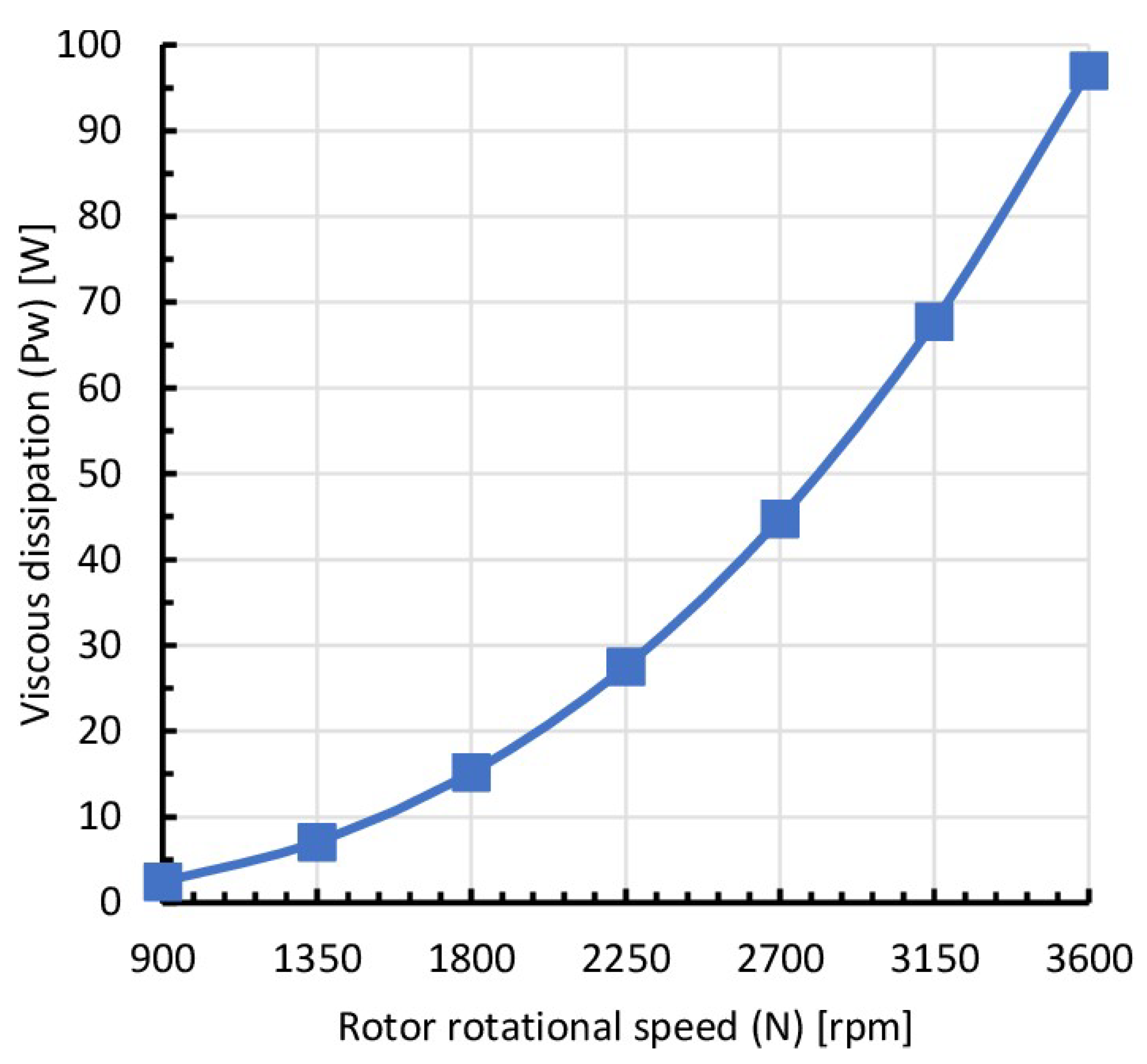
- Rotor Speed
- Motor Structural Parameters
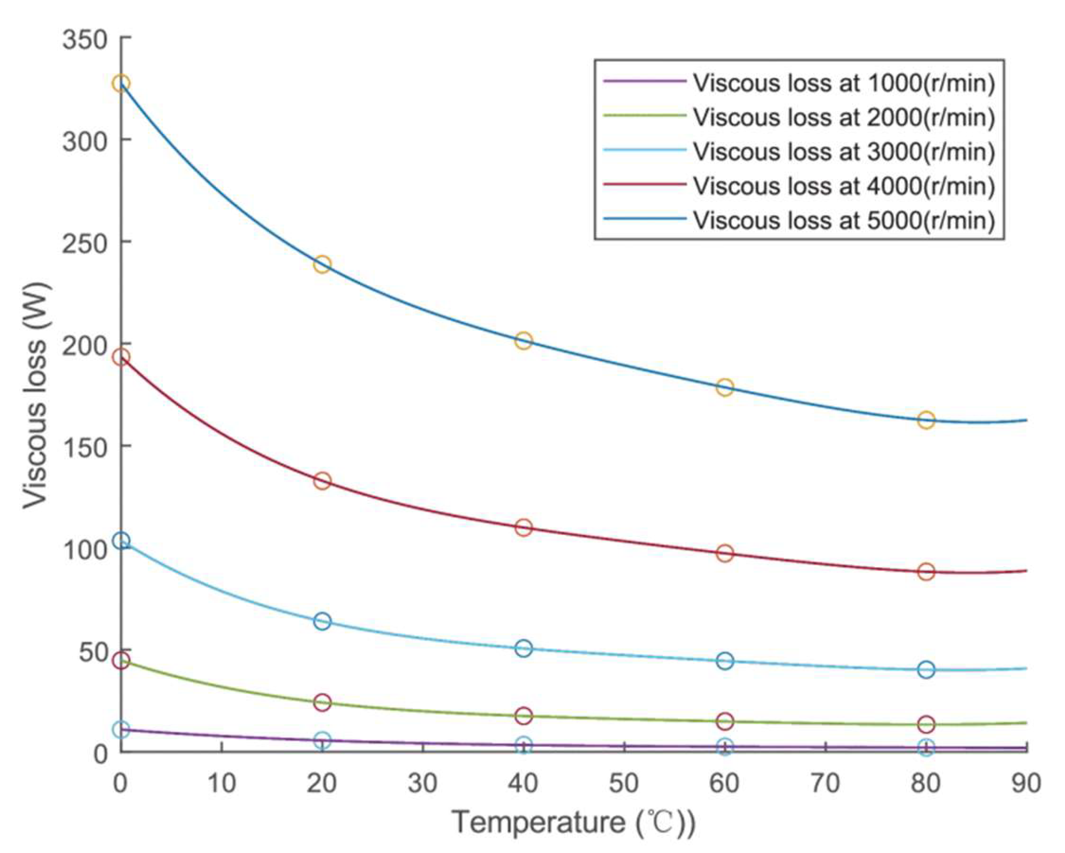
- Temperature and Viscosity
- Rotor Surface Roughness
- When the rotor surface is smooth (Ks = 0 mm), the friction coefficient Cf is given by the following:
- Zone 1: Linear theory regime (Ta < TaC1):
- Zone 2: Non-linear theory regime (TaC1 < Ta < TaC2):where Cf0 = 2.468η1/2 TaC11/2.
- Zone 3: Fully turbulent regime (Ta > TaC2):
- When the rotor surface is smooth (Ks ≠ 0 mm), the friction coefficient Cf is given by the following expression in the fully turbulent zone:where = (Ri + Ks)/Ri is the roughness ratio.
3. Progress in the Study of the Temperature Field of OFMs
3.1. Methods for Analyzing the Temperature Field
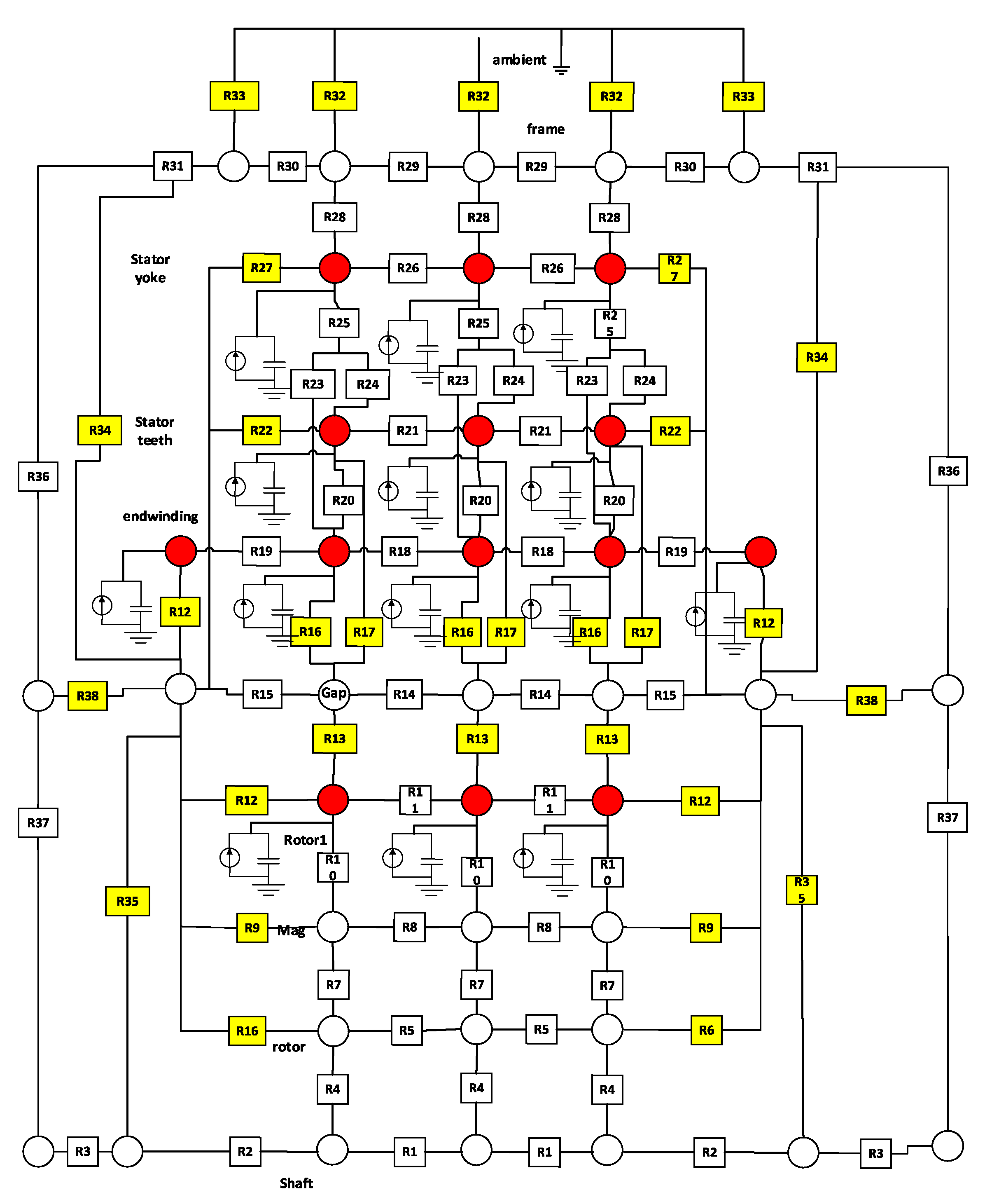
3.1.1. LPTN
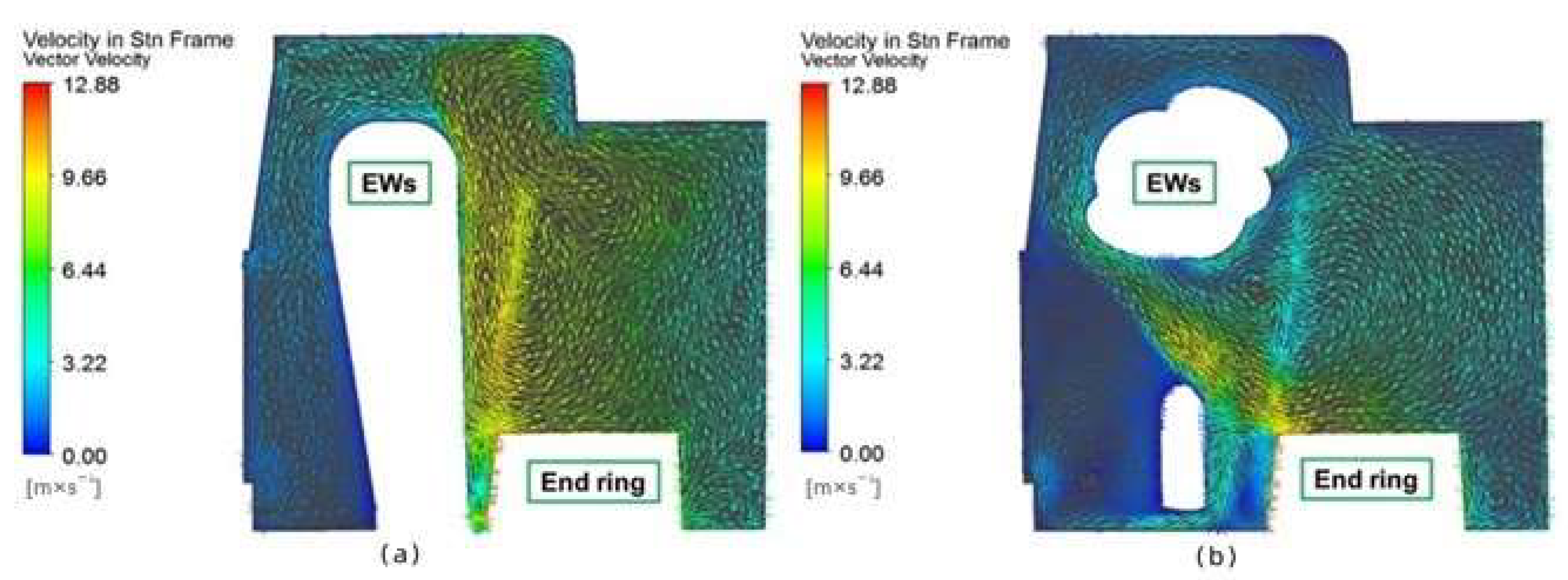
3.1.2. CFD
3.1.3. FEM
3.2. Research on the Temperature Rise in OFMs
- Set the initial temperature and, based on the corresponding viscosity of the oil at this initial temperature, perform fluid field simulation to obtain the viscous losses.
- Based on the obtained viscous losses, set the heat source in the temperature field model and calculate the temperature rise.
- Based on the average temperature of the oil calculated from the temperature rise, obtain a new value for the average viscosity of the oil, and then repeat steps 1 and 2.
4. Discussion and Future Challenges
4.1. Coupled Calculation of Viscous Losses and Temperature
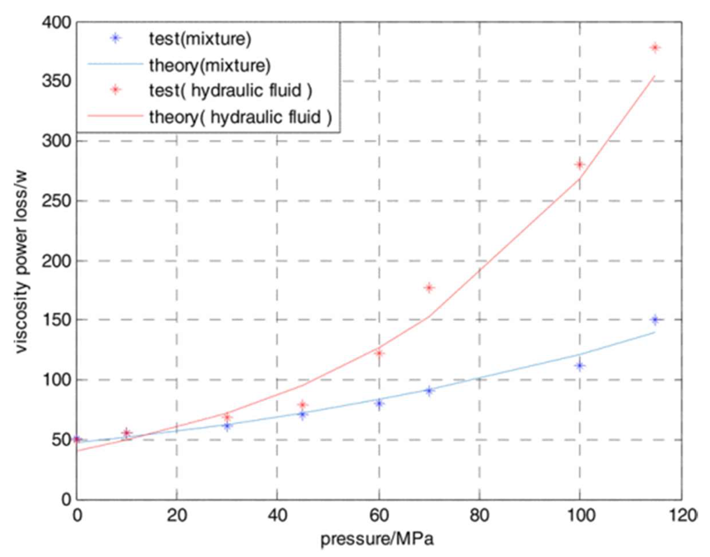
4.2. Impact of Oil Type on Viscous Losses
4.3. Influence of Rotor Surface Roughness
4.4. Influence of Motor Structural Parameters
5. Conclusions
- The use of corrected analytical formulas in CFD simulations or thermal network calculations for iterative solving, achieving fluid and temperature field coupling while enhancing computational efficiency.
- Analytical formulas for viscous loss considering temperature’s impact on oil viscosity.
- The influence of motor structural parameters and rotor surface roughness on viscous loss.
Author Contributions
Funding
Data Availability Statement
Conflicts of Interest
Abbreviations
| OFM | oil-filled motor |
| AUV | autonomous underwater vehicle |
| ROV | remotely operated vehicle |
| EHA | Electro-Hydrostatic Actuator |
| HST | hydrostatic drivetrain |
| WPMSM | wet-type permanent magnet synchronous motor |
| LPTN | Lumped-Parameter Thermal Network |
| BLDC | Brushless DC Motors |
| PMSM | permanent-magnet synchronous machine |
| SQP | Sequential Quadratic Programming |
| CFD | Computational Fluid Dynamics |
| TEFC | totally enclosed fan-cooled |
| FEM | Finite Element Method |
| HSPMM | high-speed permanent magnet motors |
| GFB | gas foil bearing |
| FEA | finite element analysis |
| EW | end winding |
| SCDM | self-contained drum motor |
| OV | oil volume percentage inside the annular area |
| VFD | variable frequency drive |
| VOF | Volume of Fluid |
| UDF | User-Defined Function |
References
- Zhang, J.; Wang, R.; Fang, Y.; Lin, Y. Insulation Degradation Analysis Due to Thermo-Mechanical Stress in Deep-Sea Oil-Filled Motors. Energies 2022, 15, 3963. [Google Scholar] [CrossRef]
- Li, D.; Guo, F.; Xu, L.; Wang, S.; Yan, Y.; Ma, X.; Liu, Y. Analysis of Efficiency Characteristics of a Deep-Sea Hydraulic Power Source. Lubricants 2023, 11, 485. [Google Scholar] [CrossRef]
- Zou, J.; Qi, W.; Xu, Y.; Xu, F.; Li, Y.; Li, J. Design of Deep Sea Oil-Filled Brushless DC Motors Considering the High Pressure Effect. IEEE Trans. Magn. 2012, 48, 4220–4223. [Google Scholar] [CrossRef]
- Bai, Y.; Zhang, Q.; Tian, Q.; Yan, S.; Tang, Y.; Zhang, A. Performance and experiment of deep-sea master-slave servo electric manipulator. In Proceedings of the CEANS 2019 MTS/IEEE, Seattle, WA, USA, 27–31 October 2019; pp. 1–5. [Google Scholar] [CrossRef]
- Ishak, D.; Manap, N.A.; Ahmad, M.S.; Arshad, M.R. Electrically actuated thrustersfor autonomous underwater vehicle. In Proceedings of the 2010 11th IEEE International Workshop on Advanced Motion Control (AMC), Nagaoka, Japan, 21–24 March 2010; pp. 619–624. [Google Scholar]
- Cho, C.P.; Fussell, B.K.; Hung, J.Y. A novel integrated electricmotor pump for underwater applications. J. Appl. Phys. 1996, 79, 5548–5550. [Google Scholar] [CrossRef]
- Hsieh, M.F.; Liao, H.J. A wide speed range sensorless control technique of brushless DC motors for electric propulsors. J. Mar. Sci. Tech. 2010, 18, 735–745. [Google Scholar] [CrossRef]
- Nagel, N. Actuation Challenges in the More Electric Aircraft: Overcoming Hurdles in the Electrification of Actuation Systems. IEEE Electrification Mag. 2017, 5, 38–45. [Google Scholar] [CrossRef]
- Sayed, E.; Abdalmagid, M.; Pietrini, G.; Sa’adeh, N.M.; Callegaro, A.D.; Goldstein, C.; Emadi, A. Review of electric machines in more-/hybrid-/ turbo-electric aircraft. IEEE Trans. Transp. Electrif. 2021, 7, 2976–3005. [Google Scholar] [CrossRef]
- Jiao, Z.; Li, Z.; Shang, Y.; Wu, S.; Song, Z.; Pan, Q. Active load sensitive electrohydrostatic actuator on more electric aircraft: Concept, design, and control. IEEE Trans. Ind. Electron. 2022, 69, 5030–5040. [Google Scholar] [CrossRef]
- Xu, J.; Du, Y.; Fang, H.; Guo, H.; Chen, Y.-H. A Robust Observer and Nonorthogonal PLL-Based Sensorless Control for Fault-Tolerant Permanent Magnet Motor with Guaranteed Postfault Performance. IEEE Trans. Ind. Electron. 2020, 67, 5959–5970. [Google Scholar] [CrossRef]
- Jiao, Z.; Li, Y.; Yu, T.; Jiang, C.; Huang, L.; Shang, Y. Dynamic thermal coupling modeling and analysis of wet electro-hydrostatic actuator. Chin. J. Aeronaut. 2022, 35, 298–311. [Google Scholar] [CrossRef]
- Yu, S. Design and Loss Analysis of High Speed Submersible Permanent Magnet Motor. Master’s Thesis, Shenyang University of Technology, Shenyang, China, 2018. [Google Scholar]
- Xiang, Y.; Tang, T.; Su, T.; Brach, C.; Liu, L.; Mao, S.S.; Geimer, M. Fast CRDNN: Towards on Site Training of Mobile Construction Machines. IEEE Access 2021, 9, 124253–124267. [Google Scholar] [CrossRef]
- Xiang, Y.; Li, R.; Brach, C.; Liu, X.; Geimer, M. A Novel Algorithm for Hydrostatic-Mechanical Mobile Machines with a Dual-Clutch Transmission. Energies 2022, 15, 2095. [Google Scholar] [CrossRef]
- Xu, J.; Jin, W.; Guo, H.; Yu, T.; Fan, W.; Jiao, Z. Modeling and analysis of oil frictional loss in wet-type permanent magnet synchronous motor for aerospace electro-hydrostatic actuator. Chin. J. Aeronaut. 2023, 36, 328–341. [Google Scholar] [CrossRef]
- Ahmed, S.; Toliyat, H.A. Coupled Field Analysis Needs in the Design of Submersible Electric Motors. In Proceedings of the 2007 IEEE Electric Ship Technologies Symposium, Arlington, VA, USA, 21–23 May 2007; pp. 231–237. [Google Scholar]
- Wenjuan, Q.; Jibin, Z.; Jianjun, L. Numerical calculation of viscous drag loss of oil-filled BLDC motor for underwater applica-tions. In Proceedings of the 2010 International Conference on Electrical Machines and Systems, Incheon, Republic of Korea, 10–13 October 2010; pp. 1739–1742. [Google Scholar]
- Jung, J.-W.; Lee, B.-H.; Kim, K.-S.; Kim, S.-I. Interior Permanent Magnet Synchronous Motor Design for Eddy Current Loss Reduction in Permanent Magnets to Prevent Irreversible Demagnetization. Energies 2020, 13, 5082. [Google Scholar] [CrossRef]
- Seeton, C.J. Viscosity–temperature correlation for liquids. Tribol. Lett. 2006, 22, 67–78. [Google Scholar] [CrossRef]
- Zhang, W.; Hu, Y.; Cao, L.; Zhuo, L.; Liu, A. Analysis and calculation of friction loss of high-speed permanent magnetic shielding motor. Trans. China Electrotech. 2023, 38, 3122–3129. [Google Scholar]
- Saari, J. Thermal Analysis of High-Speed Induction Machines. Acta Polytechnica Scandinavica Electrical Engineering Series. Ph.D. Thesis, Helsinki University of Technology, Otaniemi, Finland, 1998; 73p. [Google Scholar]
- Aglen, O. Loss calculation and thermal analysis of a high-speed generator. In Proceedings of the IEEE International Electric Machines and Drives Conference, 2003. IEMDC’03, Madison, WI, USA, 1–4 June 2003; pp. 1117–1123. [Google Scholar]
- Wendt, F. Turbulente Strmungen zwischen zwei rotierenden konaxialen Zylinderen. Ing-Arch. 1933, 9, 577–595. [Google Scholar] [CrossRef]
- Yamada, Y. Torque Resistance of a Flow between Rotating Co-Axial Cylinders Having Axial Flow. Bull. JSME 1962, 5, 634–642. [Google Scholar] [CrossRef]
- Bilgen, E.; Boulos, R. Functional Dependence of Torque Coefficient of Coaxial Cylinders on Gap Width and Reynolds Numbers. J. Fluids Eng. 1973, 95, 122–126. [Google Scholar] [CrossRef]
- Nakabayashi, K.; Yamada, Y.; Kishimoto, T. Viscous frictional torque in the flow between two concentric rotating rough cyl-inders. J. Fluid Mech. 1982, 119, 409–422. [Google Scholar] [CrossRef]
- Jianjun, L. Loss and Temperature Field Analysis for Deep-Sea Brushless DC Motor. Ph.D. Thesis, Department of Electrical Engineering, Harbin Institute of Technology, Harbin, China, 2011, unpublished. [Google Scholar]
- Escudier, M.; Oliveira, P.; Pinho, F. Fully developed laminar flow of purely viscous non-Newtonian liquids through annuli, including the effects of eccentricity and inner-cylinder rotation. Int. J. Heat Fluid Flow 2002, 23, 52–73. [Google Scholar] [CrossRef]
- Noui-Mehidi, M.N.; Ohmura, N.; Kataoka, K. Dynamics of the helical flow between rotating conical cylinders. J. Fluids Struct. 2005, 20, 331–344. [Google Scholar] [CrossRef]
- Bai, Y.; Zhang, Q.; Fan, Y.; Wang, H.; Zhang, A. Research and Experiment on Viscous Friction Power Loss of Deep-Sea Electric Manipulator. In Proceedings of the OCEANS—MTS/IEEE Kobe Techno-Oceans (OTO), Kobe, Japan, 28–31 May 2018; pp. 1–4. [Google Scholar] [CrossRef]
- Ji, Z.Q.; Zhu, B.-H.; Lou, Z.-K.; Qian, P.-C. Study of Resistant Torque for “Small Aspect Ratio” Submersible Rotor in Hydraulic Motor Pump. Chin. Hydraul. Pneum. 2018, 2, 20–26. [Google Scholar] [CrossRef]
- Jin, Z.; Zhao, L.; Zhao, X. Research on characteristics of oil immerserd motor for deep water servo application. J. Tianjin Univ. Technollogy 2021, 37, 40. [Google Scholar]
- Yongming, X.; Dawei, M.; Guohui, L. Mechanical loss analysis and calculation of diving oil motor. Electr. Mach. Control. 2004, 8, 370–372. [Google Scholar]
- Nachouane, A.B.; Abdelli, A.; Friedrich, G.; Vivier, S. Estimation of windage losses inside very narrow air gaps of high speed electrical machines without an internal ventilation using CFD methods. In Proceedings of the 2016 XXII International Conference on Electrical Machines (ICEM), Lausanne, Switzerland, 4–7 September 2016; pp. 2704–2710. [Google Scholar]
- Nachouane, A.B.; Abdelli, A.; Friedrich, G.; Vivier, S. Numerical approach for thermal analysis of heat transfer into a very narrow air gap of a totally enclosed permanent magnet integrated starter generator. In Proceedings of the 2015 IEEE Energy Conversion Congress and Exposition (ECCE), Montreal, QC, Canada, 20–24 September 2015; pp. 1749–1756. [Google Scholar]
- Kreith, F. Convection heat transfer in rotating systems. In Advances in Heat Transfer; Elsevier: Amsterdam, The Netherlands, 1969; p. 129. [Google Scholar]
- Han, B.; Liu, X.; Huang, Z.; Zhang, X.; Zhou, Y. Loss Calculation, Thermal Analysis, and Measurement of Magnetically Suspended PM Machine. IEEE Trans. Ind. Electron. 2017, 65, 4514–4523. [Google Scholar] [CrossRef]
- Huang, Z.; Fang, J.; Liu, X.; Han, B. Loss Calculation and Thermal Analysis of Rotors supported by Active Magnetic Bearings for High-speed Permanent Magnet Electrical Machines. IEEE Trans. Ind. Electron. 2015, 63, 2027–2035. [Google Scholar] [CrossRef]
- Hu, Y.; Li, L. Calculating the Oil-Filled Submersible Motor Starting Performance Based on the Fluid-Structure Interaction Meth-od. Small Spec. Electr. Mach. 2013, 41, 38–41. [Google Scholar]
- Chen, H. Research on the Deep-Ocean Pressure-Compensated Oil-Filled Motor. Master’s Thesis, Zhejiang University, Hangzhou, China, 2007. [Google Scholar]
- Li, L.; Peng, B. Analysis and Calculation of Viscous Friction Loss of Rotor of Submersible Motor. In Proceedings of the 14th Shenyang Science Annual Conference (Science, Engineering, Agriculture and Medicine), Shenyang, China, 31 August 2017. [Google Scholar]
- Wang, Y.; Kou, G.; Hu, S. Thermal modeling and analysis of oil-cooled high speed permanent magnet motor in the EHA system. In Proceedings of the CSAA/IET International Conference on Aircraft Utility Systems (AUS 2018), Guiyang, China, 19–22 June 2018. [Google Scholar]
- Cai, M.; Wu, S.; Yang, C. Effect of low temperature and high pressure on deep-sea oil-filled brushless DC motors. Mar. Technol. Soc. J. 2016, 50, 83–93. [Google Scholar] [CrossRef]
- Wrobel, R.; Vainel, G.; Copeland, C.; Duda, T.; Staton, D.; Mellor, P.H. Investigation of Mechanical Loss Components and Heat Transfer in an Axial-Flux PM Machine. IEEE Trans. Ind. Appl. 2015, 51, 3000–3011. [Google Scholar] [CrossRef]
- Teamah, A.M.; Hamed, M.S. Investigation of transient multiphase Taylor-Couette flow. Alex. Eng. J. 2022, 61, 2723–2738. [Google Scholar] [CrossRef]
- Teamah, A.M.; Hamned, M.S. Numerical and Experimental Study of The Viscous Dissipation of Oil inside the Electric Motor’s Gap. J. Fluid Flow, Heat Mass Transf. 2023, 10, 45. [Google Scholar] [CrossRef]
- Yin, Y.; Li, H.; Xiang, X. Oil Friction Loss Evaluation of Oil-Immersed Cooling In-Wheel Motor Based on Improved Analytical Method and VOF Model. World Electr. Veh. J. 2021, 12, 164. [Google Scholar] [CrossRef]
- Peng, J.; Hui, L.I.; Xuewei, X.; Yi, Y.; Bin, Y. Analytical calculation of oil friction loss taking into account action of cup-shaped rotor and teeth-grooves stator. Electr. Mach. Control. 2023, 27, 9–19. [Google Scholar]
- Meng, L.; Bo, Y.; Yuru, Z.; Lei, T. Analysis and research of oil friction loss of oil-cooled motor for aero. In Proceedings of the CSAA/IET International Conference on Aircraft Utility Systems (AUS 2022), Nanching, China, 17–20 August 2022; pp. 634–637. [Google Scholar]
- Wu, K.; Cai, L.; Zhang, J.; Fang, Y.; Wang, Y. Thermal analysis of deep-sea oil-filled motor using lumped-parameter thermal model and CFD. In Proceedings of the 2022 IEEE Transportation Electrification Conference and Expo, Asia-Pacific (ITEC Asia-Pacific), Haining, China, 28–31 October 2022; pp. 1–5. [Google Scholar]
- Liu, J.; Yan, L.; He, X.; Zhou, Y.; Yu, Z. Analysis of Oil Viscous Drag Loss of Deep-sea Motor Based on CFD Method. In Proceedings of the 2022 IEEE 17th Conference on Industrial Electronics and Applications (ICIEA), Chengdu, China, 16–19 December 2022; pp. 1289–1293. [Google Scholar]
- Cai, L. Analysis of Viscous Loss and Temperature Field of Oil-Filled Permanent-Magnet Synchronous Motor. Master’s Thesis, Zhejiang University, Hangzhou, China, 2023. [Google Scholar]
- Geng, W.; Zhu, T.; Zhang, Y.; Wu, C.; Wang, Y.; Li, Q.; Zhang, Z. Rotor Air-Friction Loss and Thermal Analysis of IPM Rotors for High Speed Axial-Flux Machine. IEEE Trans. Ind. Appl. 2022, 59, 779–788. [Google Scholar] [CrossRef]
- Boglietti, A.; Cavagnino, A.; Staton, D.; Shanel, M.; Mueller, M.; Mejuto, C. Evolution and Modern Approaches for Thermal Analysis of Electrical Machines. IEEE Trans. Ind. Electron. 2009, 56, 871–882. [Google Scholar] [CrossRef]
- Björn, J.; Johan, A.; Petter, K. Thermal Modelling of an Electro-hydrostatic Actuation System. In Proceedings of the Recent Advance in Aerospace Actuation System and Components, Toulouse, France, 13–15 June 2001. [Google Scholar]
- Jiang, Y.; Huang, X. Thermal Analysis of BLDC Motors Using Thermal Network Modeling for Aerospace Applications. Mi-cromotors 2013, 46, 19–23. [Google Scholar]
- Gronwald, P.O.; Kern, T.A. Traction Motor Cooling Systems: A Literature Review and Comparative Study. IEEE Trans. Transp. Electrif. 2021, 7, 2892–2913. [Google Scholar] [CrossRef]
- Sciascera, C.; Giangrande, P.; Papini, L.; Gerada, C.; Galea, M. Analytical Thermal Model for Fast Stator Winding Temperature Prediction. IEEE Trans. Ind. Electron. 2017, 64, 6116–6126. [Google Scholar] [CrossRef]
- Nategh, S.; Huang, Z.; Krings, A.; Wallmark, O.; Leksell, M. Thermal Modeling of Directly Cooled Electric Machines Using Lumped Parameter and Limited CFD Analysis. IEEE Trans. Energy Convers. 2013, 28, 979–990. [Google Scholar] [CrossRef]
- La Rocca, S.; Pickering, S.J.; Eastwick, C.N.; Gerada, C.; Rönnberg, K. Fluid flow and heat transfer analysis of TEFC machine end regions using more realistic end-winding geometry. J. Eng. 2019, 2019, 3831–3835. [Google Scholar] [CrossRef]
- Guo, B.; Huang, Y.; Guo, Y.; Zhu, J. Thermal Analysis of the Conical Rotor Motor Using LPTN With Accurate Heat Transfer Co-efficients. IEEE Trans. Appl. Supercond. 2016, 26, 1–7. [Google Scholar]
- Min, F.; Hai, Y.; Zhaoyang, Y.; Wenliang, W.; Chunxu, M. Coupling calculation of 3D whole domain steady flow and temperature field for underwater oil-filled brushless DC motors. In Proceedings of the 2019 22nd International Conference on Electrical Machines and Systems (ICEMS), Harbin, China, 11–14 August 2019; pp. 1–6. [Google Scholar]
- Sim, K.; Lee, Y.-B.; Jang, S.-M.; Kim, T.H. Thermal analysis of high-speed permanent magnet motor with cooling flows supported on gas foil bearings: Part I—coupled thermal and loss modeling. J. Mech. Sci. Technol. 2015, 29, 5469–5476. [Google Scholar] [CrossRef]
- Li, Z.; Zhang, Q.; Yu, R.; Zhang, L.; Xu, C. Analysis of Influence Factors of Underwater Motor Temperature Field Based on Magne-to-thermal-flux Coupling. In Proceedings of the 2018 IEEE International Conference on Mechatronics and Automation (ICMA), Changchun, China, 5–8 August 2018; pp. 773–778. [Google Scholar]
- Feng, W.; Yang, S.; Zhang, B. Research on Temperature Rise of High-Temperature Ultra-Slim Long Submersible Permanent Magnet Motor. Electr. Mach. Control. Appl. 2021, 48, 50–56. [Google Scholar]
- Zhang, X. Study on the Temperature Field of the Submersible Permanent Magnet Synchronous Motor; China University of Petroleum (EastChina): Dongying, China, 2017. [Google Scholar]
- Wang, J.; Xu, L.; Cai, L.; Zhang, J.; Tian, J. CFD-based Temperature Field Analysis and Lifetime Prediction of Brushless DC Motor. In Proceedings of the 2022 IEEE Transportation Electrification Conference and Expo, Asia-Pacific (ITEC Asia-Pacific), Haining, China, 28–31 October 2022; pp. 1–5. [Google Scholar]
- Wu, L.W. Calculation of Viscous Losses and Temperature Field Analysis for Oil-Filled Permanent Magnet Synchronous Motors Based on CFD-LPTN. Master’s Thesis, Zhejiang University, Hangzhou, China, 2024. [Google Scholar]


Disclaimer/Publisher’s Note: The statements, opinions and data contained in all publications are solely those of the individual author(s) and contributor(s) and not of MDPI and/or the editor(s). MDPI and/or the editor(s) disclaim responsibility for any injury to people or property resulting from any ideas, methods, instructions or products referred to in the content. |
© 2024 by the authors. Licensee MDPI, Basel, Switzerland. This article is an open access article distributed under the terms and conditions of the Creative Commons Attribution (CC BY) license (https://creativecommons.org/licenses/by/4.0/).
Share and Cite
Zhang, J.; Shao, Y.; Long, Y.; He, X.; Wu, K.; Cai, L.; Wu, J.; Fang, Y. Methods for the Viscous Loss Calculation and Thermal Analysis of Oil-Filled Motors: A Review. Energies 2024, 17, 4659. https://doi.org/10.3390/en17184659
Zhang J, Shao Y, Long Y, He X, Wu K, Cai L, Wu J, Fang Y. Methods for the Viscous Loss Calculation and Thermal Analysis of Oil-Filled Motors: A Review. Energies. 2024; 17(18):4659. https://doi.org/10.3390/en17184659
Chicago/Turabian StyleZhang, Jian, Yinxun Shao, Yinxin Long, Xiangning He, Kangwen Wu, Lingfeng Cai, Jianwei Wu, and Youtong Fang. 2024. "Methods for the Viscous Loss Calculation and Thermal Analysis of Oil-Filled Motors: A Review" Energies 17, no. 18: 4659. https://doi.org/10.3390/en17184659
APA StyleZhang, J., Shao, Y., Long, Y., He, X., Wu, K., Cai, L., Wu, J., & Fang, Y. (2024). Methods for the Viscous Loss Calculation and Thermal Analysis of Oil-Filled Motors: A Review. Energies, 17(18), 4659. https://doi.org/10.3390/en17184659