Two-Stage Optimal Configuration Strategy of Distributed Synchronous Condensers at the Sending End of Large-Scale Wind Power Generation Bases

Abstract

The transmission end of large-scale wind power generation bases faces challenges such as high AC-DC coupling strength, low system inertia, and weak voltage support capabilities. Deploying distributed synchronous condensers (SCs) within and around wind farms can effectively provide transient reactive power support, enhance grid system inertia at the transmission end, and improve dynamic frequency support capabilities. However, the high investment and maintenance costs of SCs hinder their large-scale deployment, necessitating the investigation of optimal SC configuration strategies at critical nodes in the transmission grid. Initially, a node inertia model was developed to identify weaknesses in dynamic frequency support, and a critical inertia constraint based on node frequency stability was proposed. Subsequently, a multi-timescale reactive power response model was formulated to quantify the impact on short-circuit ratio improvement and transient overvoltage suppression. Finally, a two-stage optimal configuration strategy for distributed SCs at the transmission end was proposed, considering dynamic frequency support and transient voltage stability. In the first stage, the optimal SC configuration aimed to maximize system inertia improvement per unit investment to meet dynamic frequency support requirements. In the second stage, the configuration results from the first stage were adjusted by incorporating constraints for enhancing the multiple renewable short-circuit ratio (MRSCR) and suppressing transient overvoltage. The proposed model was validated using the feeder grid of a large energy base in western China. The results demonstrate that the optimal configuration scheme effectively suppressed transient overvoltage at the generator end and significantly enhanced the system’s dynamic frequency support strength.

1. Introduction

1.1. Research Background

As a result of the “dual-carbon” policy and transition away from traditional energy, renewable energy units have been given access to the grid on a large scale, replacing some traditional thermal power units [1]. Wind power has the advantage of being clean and renewable compared to traditional energy sources [2]. In areas that are difficult to reach from the grid, such as mountains and deserts, wind power can reduce the dependence of these areas on the traditional grid and increase energy self-sufficiency. Wind power systems are less costly to operate in the long term, which can help these areas become economically sustainable [3]. The existing transmission-end grid of large-scale wind power generation bases is encountering various challenges, such as issues with DC commutation, frequency instability, and transient voltage fluctuations [4]. Traditional reactive power compensation devices such as static var compensators (SVCs) and static synchronous compensators (STATCOMs) have weak response and delay, which may aggravate transient overvoltage problems [5]. Large-capacity synchronous condensers (SCs) are usually installed on the busbar of a converter station, which are far away from new energy units and cannot effectively suppress transient overvoltage at the machine end.

Distributed SCs (50 Mvar) that configured in each renewable energy (RE) station and its proximity area can provide a fast reactive power response while improving system inertia and dynamic frequency support [6]. Nevertheless, the substantial upfront costs and ongoing maintenance expenses associated with SCs pose barriers to widespread adoption. Therefore, it is necessary to investigate the optimal configuration strategy at critical nodes of the transmission end in large-scale wind power generation bases.

1.2. Literature Survey

Existing research on optimizing the configuration of distributed SCs has mainly focused on the multiple renewable energy short-circuit ratio (MRSCR) and transient voltage safety threshold [7,8,9]. A distributed SC placement site selection method at the sending end grid was proposed considering DC blocking transient overvoltage constraints, but the distributed SC capacity selection model was not considered in [10]. Co-optimization of large-capacity and distributed SC capacity with the objective of transient voltage stability and maximum dissipation capacity was carried out in [11]. However, the mechanism of the SC maintaining transient voltage stability was not analyzed. The optimization configuration methods for distributed SCs were proposed to enhance the transient voltage support capacity, considering high- and low-voltage ride-through constraints for wind turbine units in [12,13]. However, only the transient reactive power characteristics of the SCs were analyzed, and the SC sub-transient reactive power output process was not considered. An SC optimal configuration method was proposed based on the effective short-circuit ratio of multiple stations, taking into account the electrical connection of each RE plants to the converter station in [14]. However, it only aimed to prevent DC commutation failure and did not consider the transient overvoltage at the machine end of the wind turbine. Based on the results of short-circuit ratio calculation of each RE station, the weak links in the RE cluster were identified, and reactive power compensation equipment was targeted to be configured in [15]. Synergistic planning of an SC and SVC for large-energy-base sending-end converter stations is proposed considering the DC blocking transient overvoltage constraints in [16]. The above studies were mostly optimized unilaterally from short-circuit ratio enhancement or transient overvoltage suppression, and they lacked an effective combination of the two indicators. The work performed in these research studies was unable to meet the comprehensive demand for MRSCR and transient voltage stabilization under current safety regulations and faced the risk of insufficient transient voltage support and high voltage ride-through failure unlisting.

However, a distributed synchronous condenser, as a synchronous motor with inertial response, can improve system inertia distribution and provide dynamic frequency support at the transmission end of large-scale wind power generation bases. In [17], the principle of inertia response of the synchronous condenser was analyzed, and its impact on dynamic frequency support was explored. A strategy for configuring energy storage in the sending-end power grid to enhance dynamic frequency support was proposed in [18], but the configuration of the synchronous condenser and its transient voltage stability were not studied. In [19], a node inertia index was proposed to quantitatively analyze the ability of RE stations’ nodes to resist frequency changes, but the role of the synchronous condenser in improving node inertia was not analyzed. In [20], the frequency stability constraint was transformed into critical inertia, thus clarifying the weak links affecting frequency stability from the perspective of inertia. Moreover, the model for the siting and sizing of the synchronous condenser was not studied in the aforementioned studies.

1.3. Research Focus and Organization

Therefore, this study concentrates on the optimal configuration of distributed synchronous condensers (SCs) at the transmission end of large-scale wind power generation bases, addressing some of the limitations in the existing research. These limitations include the following:

(1)

Insufficient depth in the analysis of the DC reactive power demand and the reactive power output of the SC during various transient stages post-fault, coupled with a lack of detailed examination of the coupling relationship across different time scales. This paper introduces a reactive power output model for distributed regulators from both transient and sub-transient perspectives and quantitatively assesses the influence of distributed SC integration on short-circuit ratio (SCR) enhancement and transient overvoltage suppression capabilities.

(2)

Current research has overlooked the impact of optimal distributed SC allocation on inertia enhancement and dynamic frequency support. This paper examines the effect of distributed SC integration on the dynamic inertia response of new energy bases at the sending end. The dynamic frequency support characteristics of large energy bases are analyzed based on the nodal inertia model, and a critical inertia constraint is proposed that is grounded in frequency stability considerations.

(3)

Existing optimization objectives are predominantly analyzed from a single perspective, either focusing on SCR enhancement or transient overvoltage suppression, which fails to address the comprehensive requirements for MRSCR and transient voltage stability. In this paper, a two-stage optimal configuration strategy for distributed SCs at the transmission end is proposed, considering dynamic frequency support and transient voltage stability. In the first stage, the optimal SC configuration aims to maximize system inertia improvement per unit investment to meet dynamic frequency support requirements. The second stage adjusts the configuration results from the first stage by incorporating constraints for enhancing the MRSCR and suppressing transient overvoltage.

This article is organized as follows. A node inertia model is developed to identify weaknesses in dynamic frequency support, and a critical inertia constraint based on node frequency stability is proposed in Section 2. Subsequently, a multi-timescale reactive power response model is formulated to quantify the impact on short-circuit ratio improvement and transient overvoltage suppression in Section 3. A two-stage optimal configuration strategy for distributed SCs at the transmission end is proposed, considering dynamic frequency support and transient voltage stability in Section 4. The proposed model is validated using the feeder grid of a large energy base in western China in Section 5. Finally, conclusions and limitations of the analysis provided in this article are presented in Section 6.

2. Dynamic Frequency Support Capability Analysis for Considering SC Accessing of Large-Scale Wind Power Generation Bases Based on Node Inertia Modeling

Distributed SCs are configured in each RE station, and the proximity area of each RE station can provide a fast reactive power response while improving system inertia and dynamic frequency support. This section examines the effect of distributed SC integration on the dynamic inertia response at the sending end of new energy bases. The dynamic frequency support characteristics of large energy bases are analyzed based on the nodal inertia model, and a critical inertia constraint is proposed that is grounded in frequency stability considerations.

2.1. Dynamic Inertial Response Model for Considering SC Accessing of Large-Scale Wind Power Generation Bases

Unlike the rotor motion generator theory of traditional thermal power units, the output power of RE units is only related to natural factors (e.g., wind speed, solar intensity) and is not related to system frequency changes. In addition, RE units that have been given access to the grid widely use power electronic components, such as converters, so that the active power is decoupled from the frequency change. At the same time, RE units do not have rotational inertia. Assuming that there are N synchronous generators and M RE units in a system, the equivalent inertia of the system H_eq can be expressed as follows.

$$\begin{gathered} H_{eq}={\displaystyle \frac{{\displaystyle \sum _{n=1}^N{J}_n{w}_n^2+{\displaystyle \sum _{w=1}^W{H}_w}}}{2({\displaystyle \sum _{n=1}^N{S}_n}+{\displaystyle \sum _{m=1}^M{S}_m+{\displaystyle \sum _{w=1}^W{S}_w})}}} \\ {H}_w=K_{0,w}-(K_{0,w}-K_{\infty ,w}){\displaystyle \frac{1}{T_{w}s+1}} \end{gathered}$$

(1)

where J_i and w_i represent the rotational inertia and rated speed of the i-th synchronous generator; S_i, S_j, and S_w represent the rated capacity of the synchronous generator, the RE unit, and asynchronous wind turbine, respectively. H_w represents the rotational inertia of the w-th asynchronous wind turbine. K_0,w and $K_{\infty ,w}$ represent proportionality coefficients at the moment of perturbation and steady state. T_w represents the inertia time constant of the w-th asynchronous wind turbine. It can be seen that a large number of RE units that have been given access to the grid will lead to a reduction in the system inertia level and a weakening of the regulating frequency capability, which seriously threatens the system frequency safety. The equivalent inertia H_eq′ after the access of distributed SCs is shown in (2).

$$H_{{eq}^{\prime }}={\displaystyle \frac{{\displaystyle \sum _{n=1}^N{J}_n{w}_n^2}+{\displaystyle \sum _{k=1}^K{J}_k{w}_k^2+{\displaystyle \sum _{w=1}^W{H}_w}}}{2({\displaystyle \sum _{n=1}^N{S}_n}+{\displaystyle \sum _{m=1}^M{S}_m}+{\displaystyle \sum _{w=1}^W{S}_w}+{\displaystyle \sum _{k=1}^K{S}_k})}}$$

(2)

where K is the number of distributed SCs connected to the system; J_k, w_k, and S_k represent the rotational inertia, rated speed, and rated capacity of the k-th SC. The dynamic frequency response of the system is expressed in the form of rotor motion equation as follows.

$$2H_{{eq}^{\prime }}{\displaystyle \frac{d{f}_{cen}}{dt}}=-D{f}_{cen}-\Delta P_{dis}+\Delta P_m$$

(3)

where D represents the system damping coefficient. ΔP_dis and ΔP_m represent the instantaneous disturbance power and the mechanical power added by the synchronous motor, respectively; f_cen represents the center of inertia frequency. When there is an active sudden change in the system, the inertia of the distributed regulator and the synchronous motor provides a damping effect based on the synchronous power coefficient for the instantaneous change in frequency, which effectively slows down the rate of frequency drop and improves the system’s ability to resist disturbances. However, since the distributed regulator is not dragged by the prime mover, the rotational speed is slower than that of the synchronous motor, resulting in active power phase lag, which delays the emergence of the lowest point of frequency in the center of inertia.

2.2. Dynamic Frequency Support Analysis of Large Energy Bases Based on Nodal Inertia Modeling

The disturbance power will be distributed among the synchronous generators according to the synchronous power coefficient, resulting in the speed of each synchronous generator not being exactly the same. The difference in dynamic frequency of each node reflects the spatial and temporal distribution of the system frequency. The node inertia model is proposed to describe the node frequency–disturbance–resistant characteristics that can reflect the weakness of the system dynamic frequency. The inertia H_p of any node p is defined as the system disturbance power ΔP_dis-p divided by the value of the node p frequency change.

$$H_p={\displaystyle \frac{\Delta P_{dis-p}}{2\frac{d{f}_p}{dt}}}$$

(4)

where f_p represents the frequency of node p. However, there is no inertia at node p itself, which is the embodiment of the total inertia of the synchronous generator and the distributed SC according to the synchronous power coefficient. Therefore, assuming that a sudden change in active power occurs at node k, the sudden change in power ΔP_dis-j shared by the synchronous generator or SC j can be expressed as follows.

$$\Delta P_{dis-j}=\Delta P_{dis}{\displaystyle \frac{{\phi }_{jk}}{{\displaystyle \sum _{j\in J}{\phi }_{jk}}}}$$

(5)

where J is the set of synchronous generator and SC access nodes. The synchronous power coefficient φ_jk can be expressed as follows.

$${\phi }_{jk}=U_j{U}_k{B}_{jk}\cos {\delta }_{jk0}$$

(6)

where U_j and U_k represent the pre-disturbance voltage amplitudes, respectively; δ_jk0 represents the pre-disturbance phase angle difference between nodes j and k before the disturbance. B_jk represents the pre-disturbance electricana of node j and fault node k. The dynamic frequency change rate of the synchronous generator or SC j can be expressed as follows.

$${\displaystyle \frac{d{f}_j}{dt}}={\displaystyle \frac{{\phi }_{jk}\Delta P_{dis}}{2H_j{\displaystyle \sum _{j\in J}{\phi }_{jk}}}}$$

(7)

As for the calculation of inertia H_p for any node p within the sending-end system, the node network equations need to be established first as follows.

$$\left[\begin{array}{c}{\mathit{I}}_{\mathit{J}}\\ \mathbf{0}\end{array}\right]={\mathit{Y}}_{\mathit{s}}\left[\begin{array}{c}{\mathit{U}}_{\mathit{J}}\\ {\mathit{U}}_{\mathit{P}}\end{array}\right]=\left[\begin{array}{c}\begin{array}{cc}{\mathit{Y}}_{\mathit{J}\mathit{J}}& {\mathit{Y}}_{\mathit{j}\mathit{P}}\end{array}\\ \begin{array}{cc}{\mathit{Y}}_{\mathit{P}\mathit{J}}& {\mathit{Y}}_{\mathit{P}\mathit{P}}\end{array}\end{array}\right]\left[\begin{array}{c}{\mathit{U}}_{\mathit{J}}\\ {\mathit{U}}_{\mathit{P}}\end{array}\right]$$

(8)

where U_J and U_P represent the voltage vectors of the synchronous generator or SC accessing node j and p, respectively. Y_s represents the node broadening conductance matrix; Y_JJ, Y_PP, Y_JP, and Y_PJ represent the self-conductance and mutual conductance of the node broadening conductance matrix.

The voltage vector U_p at node p can be represented by the node j voltage vector of the synchronous generator or SC accessing.

$$U_p{e}^{j{\delta }_p}={\displaystyle \sum _{j\in J}{[-Y_{PP}^{-1}{Y}_{PJ}]}_{pj}}{U}_j{e}^{j{\delta }_j}$$

(9)

where δ_j and δ_p represent the corresponding phase angles of nodes j and p, respectively. Since sin(δ_p − δ_j) ≈ δ_p − δ_j, the phase angle of node p can be simplified as follows.

$${\delta }_p={\displaystyle \frac{{\displaystyle \sum _{j\in J}{[-Y_{PP}^{-1}{Y}_{PJ}]}_{pj}}{U}_j{\delta }_j}{U_p}}$$

(10)

Then, the frequency change corresponding to node p can be expressed as follows.

$${\displaystyle \frac{d{f}_p}{dt}}={\displaystyle \frac{{\displaystyle \sum _{j\in J}{[-Y_{PP}^{-1}{Y}_{PJ}]}_{pj}}{U}_j}{U_p}}{\displaystyle \frac{d{f}_j}{dt}}$$

(11)

The steady state node voltage amplitude variations are very small compared to the transient variations, which can be approximated as U_j ≈ U_k ≈ U_p. Eventually, the computed inertia H_p at node p can be obtained as follows.

$$H_p={\displaystyle \frac{{\displaystyle \sum _{j\in J}{H}_j{B}_{jp}}}{{\displaystyle \sum _{j\in J}{[-Y_{PP}^{-1}{Y}_{PJ}]}_{pj}{B}_{jp}}}}$$

(12)

The node inertia H_p is only related to the synchronous generator or SC’s own inertia and the electrical distance between node j and p. Due to the uneven distribution of inertia under active perturbations, the node with the smallest system inertia is the weakest link in dynamic frequency support, and, therefore, it has the highest risk of frequency instability.

2.3. Inertia Modeling of Large Energy Bases Based on Frequency Stability Constraints

The indicators describing the dynamic stability of the system frequency mainly include the maximum frequency deviation (Δf_dis-max) and the maximum change rate of frequency (RoCoF_dis-max). The former constrains the amplitude of system frequency perturbation, while the latter constrains the rate of change in frequency. Exceeding either constraint will trigger frequency instability. Therefore, the critical inertia of large energy bases can be quantitatively assessed using these two frequency constraints.

2.3.1. Critical Inertia Modeling Based on Frequency Maximum Deviation Δf_dis-max

The maximum magnitude of frequency perturbation is primarily related to the primary frequency modulation capability and system inertia. To ensure that the maximum system frequency deviation (Δf_dis-max) remains within the specified constraints, sufficient inertia must be maintained to handle various perturbations. The system frequency variation depends on the perturbation power, system inertia, and the timing of perturbation removal [21]. The critical inertia $H_{\Delta f}^{\mathit{min}}$ based on the maximum frequency deviation Δf_dis-max is expressed as follows.

$$H_{\Delta f}^{\mathit{min}}={\displaystyle \frac{t_q{f}_s\Delta P_{dis}}{8\pi \Delta f_{max}}}$$

(13)

where f_s represents the reference frequency. t_q represents the moment of disturbance removal. Δf_max represents the maximum frequency deviation required by the national standard.

2.3.2. Critical Inertia Modeling Based on the Maximum Change Rate of Frequency RoCoF_dis-max

When the sending-end grid experiences a significant disturbance, if the maximum change rate of frequency (RoCoF_dis-max) is too high, it can cause the disconnection of RE units and damage to synchronous generators. The maximum change rate of frequency RoCoF_dis-max is expressed as follows.

$${{\displaystyle \frac{d\Delta f}{dt}}|}_{t=0}={\displaystyle \frac{-f_s\Delta P_{dis}}{2H_{RoCoF}^{\mathit{min}}{S}_b}}$$

(14)

where S_b represents the system capacity. The maximum change rate of frequency occurs at the moment of disturbance (t = 0), assuming the mechanical power and damping of the synchronous generators are negligible. The expression for the critical inertia $H_{RoCoF}^{\mathit{min}}$ is as follows.

$$H_{RoCoF}^{\mathit{min}}={\displaystyle \frac{-f_s\Delta P_{dis}}{2RoCo{F}_{max}{S}_b}}$$

(15)

where RoCoF_max represents the maximum change rate of frequency required by the national standard. In summary, the critical inertia of a large energy base, based on frequency stability constraints, should be the maximum value of the critical inertia of the above two indicators.

$$H_{\mathit{max}}=\mathit{max}\left\{{\displaystyle \frac{t_q{f}_s\Delta P_{dis}}{8\pi \Delta f_{max}}},{\displaystyle \frac{-f_s\Delta P_{dis}}{2RoCo{F}_{max}{S}_b}}\right\}$$

(16)

Therefore, it is necessary to compare the inertia of each node with the critical inertia. If a node’s inertia is smaller than the critical inertia, it represents a weak link in dynamic frequency support. In such cases, it is necessary to configure a regulator or remove part of the new energy unit to meet the inertia requirements.

3. Short-Circuit Ratio Enhancement and Transient Overvoltage Suppression Analysis for Considering SC Accessing of Large-Scale Wind Power Generation Bases

Regarding the impact of distributed SC access on transient voltage stability, this section establishes a multi-time-scale reactive power response model of distributed regulators and quantitatively analyzes the impact of regulator access on short-circuit ratio enhancement and transient overvoltage suppression capability.

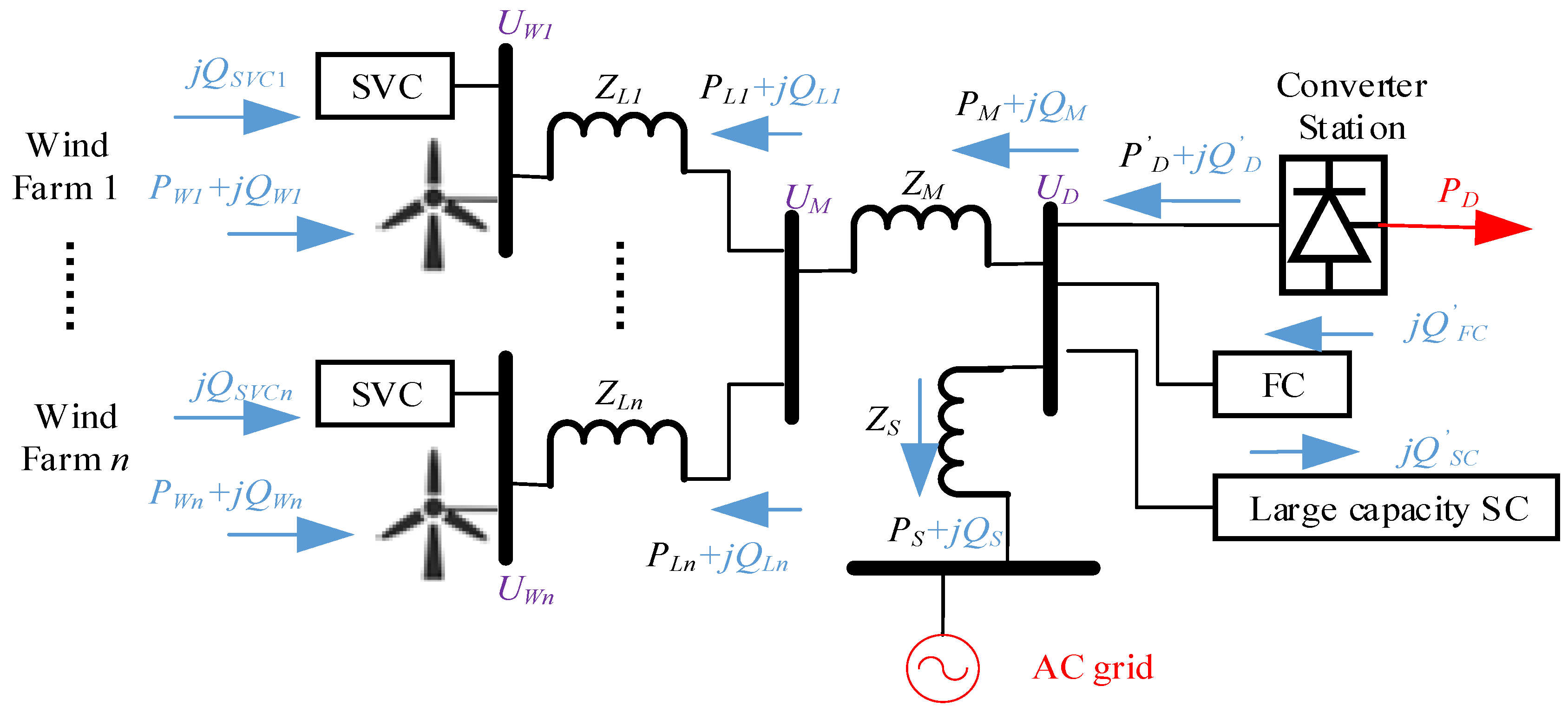
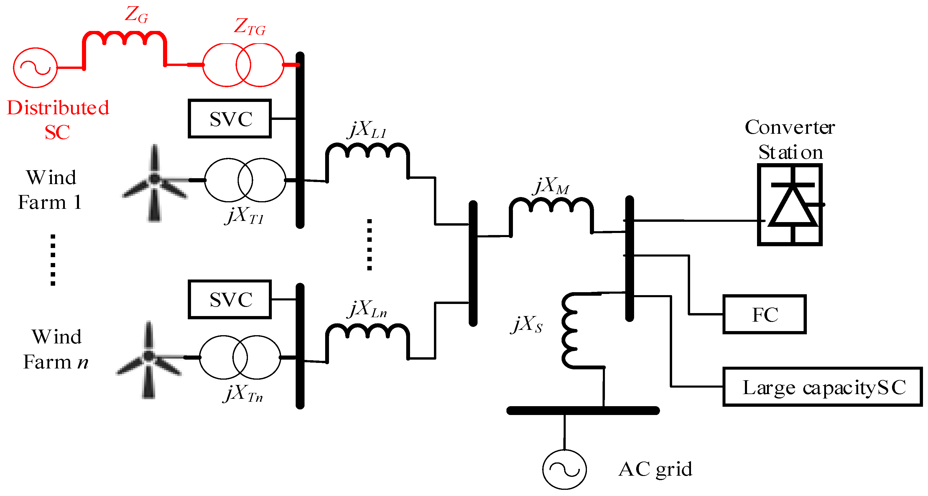
3.1. Transient Overvoltage Suppression Analysis for Considering SC Accessing of Renewable Energy Convergence Areas

3.1.1. Transient Overvoltage Conduction Mechanism for Considering SC Accessing of Renewable Energy Convergence Areas

The transient low voltage process has been discussed in [22,23]. This section focuses on analyzing the transient overvoltage conduction mechanism in new energy convergence areas. The method proposed in this paper is only applicable to the optimal allocation of the SCs at the transmission end of large energy bases connected to the UHV DC network. Therefore, the transient equivalent network of large energy base pooling areas under phase change failure is depicted in Figure 1.

During the transient process of phase change failure in an ultra-high voltage (UHV) converter station, reactive power flows in the opposite direction compared to active power, from the converter station end to the turbine end. The reactive power balance at converter station D is as follows:

$$Q_M^{\prime }+Q_S^{\prime }=Q_D^{\prime }+Q_{FC}^{\prime }-Q_{SVC}^{\prime }$$

(17)

As the bus voltage U_D rises during the transient process at the rectifier station, the filter capacitor will emit a large amount of reactive power $Q_{FC}^{\prime }$. At this time, the large-capacity SC will not be able to offset the surplus reactive power $Q_{SVC}^{\prime }$ by running in the late phase. The surplus reactive power will return from the converter station D bus to the converging station M bus. The converging station bus voltage $U_M^{\prime }$ and reactive power change $\Delta Q_M^{\prime }$ can be expressed as follows.

$$\begin{array}{l}\Delta Q_M^{\prime }=(Q_M^{\prime }-Q_{XL}^{\prime })-(Q_M-Q_{XL})<0\\ U_M^{\prime }=U_M-{\displaystyle \frac{\Delta Q_M^{\prime }}{S_M}}\\ Q_{XL}^{\prime }={\displaystyle \sum _{n=1}^N{Q}_{Ln}^{\prime }}={\displaystyle \sum _{n=1}^N[Q_{Wn}^{\prime }}+{\displaystyle \frac{{(P_{Wn}^{\prime })}^2+{(Q_{Wn}^{\prime })}^2}{{(U_{Wn}^{\prime })}^2}}{Z}_L]\end{array}$$

(18)

where U_M and Q_M represent the steady-state converging station bus voltage and reactive power output. The increase in the converging station bus voltage will be transmitted to the wind farms, resulting in transient overvoltage.

$$U_{Wn}^{\prime }=U_{Wn}-{\displaystyle \frac{\Delta Q_{Ln}^{\prime }-\Delta Q_{Wn}^{\prime }-\Delta Q_{SVCn}^{\prime }}{S_{Wn}}}$$

(19)

Each wind farm bus is generally equipped with an SVC or a distributed capacitor. The reactive power output capability is proportional to the square of the bus voltage to which it is connected. When the system is in steady state, it is able to supplement the system reactive power at a fixed value. However, it is more likely to cause transient overvoltage at the machine end when reactive power return occurs. The severity is related to the capacity of the reactive power compensation device and the wind farms’ control strategy.

3.1.2. Transient Voltage Stabilization Mechanism of Distributed SC Accessing in Multiple Time Scales

Similar to synchronous generators, the sub-transient process of the distributed SC is dominated by the damping winding. When the damping winding decays dynamically, the SCs enter a transient process dominated by the excitation winding and the excitation regulator. Since the SCs do not carry an active load, δ ≈ 0, and the SCs mostly have a hidden pole structure, X_d ≈ X_q, the SCs’ power can thus be expressed as follows:

$$\{\begin{array}{c}{P}_{SC}=u_d{i}_d+u_q{i}_q\approx {\displaystyle \frac{E_q{U}_d}{X_d}}\sin \delta \approx 0\\ Q_{SC}=u_q{i}_d-u_d{i}_q\approx u_q{i}_d\approx U_s{i}_d\end{array}$$

(20)

When excitation regulation is not considered in the sub-transient stage, the voltage drops at the SC terminal after a system short circuit, Δu_d = u_d − u_d0, Δu_q = u_q − u_q0 ≈ U_s1 − U_s0. Therefore, it is linked with the magnetic chain equation.

$$\{\begin{array}{c}{\psi }_d=-\Delta u_d=p{\psi }_d-{\psi }_q-r{i}_d\\ {\psi }_q=-\Delta u_q=p{\psi }_q-{\psi }_d-r{i}_q\end{array}$$

(21)

Solving for the d-axis current variation Δi_d, and taking its Laplace inverse transform while superimposing the steady-state components, the time-domain expression is expressed as follows:

$$\Delta i_d=-\Delta U_s\left[\left({\displaystyle \frac{1}{X_d^{″}+X_{TG}}}-{\displaystyle \frac{1}{X_d^{\prime }+X_{TG}}}\right)e^{-{\displaystyle \frac{t}{T_d^{″}}}}+\left({\displaystyle \frac{1}{X_d^{\prime }+X_{TG}}}-{\displaystyle \frac{1}{X_d+X_{TG}}}\right)e^{-{\displaystyle \frac{t}{T_d^{\prime }}}}-{\displaystyle \frac{\cos (\omega t+\delta )}{X_d^{″}+X_{TG}}}{e}^{-{\displaystyle \frac{t}{T_a}}}+{\displaystyle \frac{1}{X_d+X_{TG}}}\right]$$

(22)

where $X_d^{″}$ and $T_d^{″}$ represent the d-axis sub-transient reactance and short-circuit time constant, respectively. $X_d^{\prime }$ and $T_d^{\prime }$ represent the d-axis transient reactance and short-circuit time constant, respectively. T_a represents the time constant of the stator non-periodic component. ΔU_s represents the drop value of the bus voltage. X_TG represents the transformer reactance at the SC outlet. Therefore, the reactive power response variation in the distributed SC during the sub-transient stage can be expressed as follows:

$$\Delta Q_{SC}^{″}=-U_{s1}\Delta U_s\left[{\displaystyle \frac{\cos (\omega t+\delta )}{X_d^{″}+X_{TG}}}{e}^{-{\displaystyle \frac{t}{T_a}}}-\left({\displaystyle \frac{1}{X_d^{″}+X_{TG}}}-{\displaystyle \frac{1}{X_d^{\prime }+X_{TG}}}\right)e^{-{\displaystyle \frac{t}{T_d^{″}}}}-\left({\displaystyle \frac{1}{X_d^{\prime }+X_{TG}}}-{\displaystyle \frac{1}{X_d+X_{TG}}}\right)e^{-{\displaystyle \frac{t}{T_d^{\prime }}}}\right]+{\displaystyle \frac{U_{s0}\Delta U_s}{X_d+X_{TG}}}$$

(23)

From the (23) first term, it is evident that the variation in the distributed SC reactive power response is inversely related to the voltage variation. Furthermore, the transient dynamic reactive power support capability can instantaneously issue or absorb a large amount of reactive power, effectively inhibiting transient voltage fluctuations and preventing the failure of UHV sending-end commutation and large-scale unlinking of RE units.

In the transient characteristic analysis, the inertia link of the excitation system is expressed as follows since the excitation structure of the distributed SCs mostly adopts the self-parallel excitation method.

$$\Delta E_f={\displaystyle \frac{K_a\Delta U_s}{1+Ts}}$$

(24)

where T represents the control time constant of the excitation system, which is negligible; K_a represents the strong excitation multiplier of the excitation system, with a maximum of 2.5. ΔE_f represents the hypothetical no-load potential change. Additionally, the stator and rotor equations of the SCs during the transient phase can be expressed as follows.

$$E_q^{\prime }=U_s+X_d^{\prime }{i}_d$$

(25)

$$T_d^{\prime }{\displaystyle \frac{d{E}_q^{\prime }}{dt}}=E_f-E_q^{\prime }-(X_d-X_d^{\prime })i_d$$

(26)

Substituting (24) into (25) and (26), the d-axis current variation Δi_d, frequency domain expression is expressed as follows.

$$\Delta i_d=-{\displaystyle \frac{\Delta U_s\left(\frac{K_a+1}{X_d+X_{TG}}-\frac{1}{X_d^{\prime }+X_{TG}}\right)}{1+\frac{X_d^{\prime }+X_{TG}}{X_d+X_{TG}}{T}_d^{\prime }s}}-{\displaystyle \frac{\Delta U_s}{X_d^{\prime }+X_{TG}}}$$

(27)

At this point, the reactive power response variation in the distributed SCs during the transient phase can be expressed as follows:

$$\Delta {Q^{\prime }}_{SC}=-{\displaystyle \frac{U_{s1}\Delta U_s\left(\frac{1}{X_d^{\prime }+X_{TG}}-\frac{K_a+1}{X_d+X_{TG}}\right)}{1+\frac{X_d^{\prime }+X_{TG}}{X_d+X_{TG}}{T}_d^{\prime }s}}+{\displaystyle \frac{U_{s1}\Delta U_s}{X_d^{\prime }+X_{TG}}}$$

(28)

Apart from the second SCs’ spontaneous reactive power response, the strong excitation control of the excitation system will counteract the voltage fluctuation while maintaining transient voltage stability.

Distributed SCs access suppresses transient overvoltages in the sub-transient and transient phases. In the sub-transient and transient phases, given that the sub-transient time constant is $T_d^{″}$ ≈ 0.05 s, the excitation system’s strong excitation reaches its maximum multiplier in about 0.05 s. Within the first 0.05 s of the fault occurrence, the SC absorbs/generates transient reactive power under sub-transient action, and its output is opposite to the bus voltage change from (23).

Subsequently, the system enters a transient phase dominated by excitation control action, and under strong excitation, its reactive power output can continue to provide transient voltage support for the bus and sustain this output for an extended period, thereby accelerating bus voltage recovery from (28).

3.2. MRSCR Index Impact Analysis for Considering SC Accessing of Renewable Energy Convergence Areas

The index MRSCR considers the electrical interconnection between each wind farm, enabling a quantitative assessment of transient voltage support strength. In this section, the index MRSCR is employed to evaluate the impact of distributed SC access on the transient voltage support strength of large wind power generation bases.

The node impedance matrix represents the simplified AC equivalent network at the sending end of large wind power generation bases, which is expressed as follows.

$$\left[\begin{array}{c}{\mathit{U}}_{\mathit{R}1}\\ {\mathit{U}}_{\mathit{R}2}\\ ⋮\\ {\mathit{U}}_{\mathit{R}\mathit{n}}\end{array}\right]=\left[\begin{array}{cccc}{\mathit{Z}}_{11}& {\mathit{Z}}_{12}& \cdots & {\mathit{Z}}_{1\mathit{n}}\\ {\mathit{Z}}_{21}& {\mathit{Z}}_{22}& \cdots & {\mathit{Z}}_{2\mathit{n}}\\ ⋮& ⋮& \ddots & ⋮\\ {\mathit{Z}}_{\mathit{n}1}& {\mathit{Z}}_{\mathit{n}2}& \cdots & {\mathit{Z}}_{\mathit{n}\mathit{n}}\end{array}\right]\left[\begin{array}{c}{\mathit{I}}_{\mathit{R}1}\\ {\mathit{I}}_{\mathit{R}2}\\ ⋮\\ {\mathit{I}}_{\mathit{R}\mathit{n}}\end{array}\right]$$

(29)

where U_Ri and I_Ri represent the injected system current and bus voltage vectors for the transient process of RE stations, respectively. Z_ij represents the node impedance matrix, which is related to the network structure and parameters. The MRSCR of the new energy stations can be expressed as follows.

$$MRSC{R}_i={\displaystyle \frac{\left|U_{Mi}\right|}{\left|U_{Ri}\right|}}={\displaystyle \frac{\left|U_{Mi}\right|}{\left|Z_{ii}{I}_{Ri}+{\displaystyle \sum _{j=1,j\ne i}^n{Z}_{ij}{I}_{Rj}}\right|}}$$

(30)

where U_Mi represents the grid-accessed rated voltage of RE stations. By multiplying the numerator and the denominator by U^*_Ri/Z_ii, the simplified index MRSCR can be expressed as follows.

$$MRSC{R}_i={\displaystyle \frac{\left|U_{Ri}^{*}{U}_{Mi}/Z_{ii}\right|}{\left|U_{Ri}^{*}{I}_{Ri}+{\displaystyle \sum _{j=1,j\ne i}^n\frac{Z_{ij}}{Z_{ii}}{I}_{Rj}}\right|}}={\displaystyle \frac{S_i}{P_{Ri}+{\displaystyle \sum _{j=1,j\ne i}^n\frac{Z_{ij}{U}_{Ri}^{*}}{Z_{ii}{U}_{Rj}^{*}}}{P}_{Rj}}}$$

(31)

After an RE unit node p is accessed to the SC, the large energy base network is equivalent to adding a branch circuit with impedance Z_SC, which includes the transformer impedance Z_TG at the SC outlet and the SC self-impedance Z_G, as shown by the red line in Figure 2.

Consequently, the mutual impedance $Z_{ij}^{\prime }$ in the node impedance matrix after the SC accessing can be expressed as follows.

$$Z_{ij}^{\prime }=Z_{ij}-{\displaystyle \frac{Z_{pi}{Z}_{pj}}{Z_{pp}+Z_{SC}}}$$

(32)

Accessing the distributed SC at node p reduces all mutual impedance in the matrix, thereby increasing the MRSCR as indicated by (30). To quantitatively analyze the impact on accessing the distributed SC of the index ΔMRSCR change, the index ΔMRSCR before and after accessing the SC is used to take the partial derivative of the mutual impedance Z_pi, and the results are shown as follows.

$${\displaystyle \frac{\partial \Delta MRSCR}{\partial Z_{pi}}}={\displaystyle \frac{\partial [\frac{S_i}{P_{Ri}+{\displaystyle \sum _{j=1,j\ne i}^n\frac{Z_{ij}^{\prime }{U}_{Ri}^{*}}{Z_{ii}{U}_{Rj}^{*}}}{P}_{Rj}}]}{\partial Z_{pi}}}={\displaystyle \frac{U_{Ri}^2{\displaystyle \sum _{j=1}^n\left|Z_{pj}^{\prime }\right|}{P}_{Rj}}{\left|Z_{pp}+Z_{ii}\right|{\left[{\displaystyle \sum _{j=1}^n\left|Z_{ij}^{\prime }\right|}{P}_{Rj}-\left|\frac{Z_{pi}^{\prime }}{Z_{pp}+Z_{ii}}\right|{\displaystyle \sum _{j=1}^n\left|Z_{pj}^{\prime }\right|}{P}_{Rj}\right]}^2}}$$

(33)

The larger the mutual impedance of node p with other nodes, the more significant the MRSCR enhancement. Conversely, the further the node is electrically distant in a large new energy base, the smaller the MRSCR value of that node. Therefore, the distributed SCs should be configured at nodes with smaller MRSCR values to maximize the SCR of the large energy base convergence area.

4. Materials and Methods: Two-Stage Optimal Configuration Strategy of Distributed SCs at the Sending End of Large-Scale Wind Power Generation Bases Considering the Profit Balance of Multiple Actors under Joint Market Trading

The two-stage optimal configuration of SC for large-scale wind power generation bases is proposed by considering dynamic frequency support and transient voltage stability. The configuration is divided into two phases. In the first stage, the optimal SC configuration aims to maximize system inertia improvement per unit investment to meet dynamic frequency support requirements. The second stage adjusts the configuration results from the first stage by incorporating constraints for enhancing the MRSCR and suppressing transient overvoltage.

4.1. Stage 1: Distributed SC Configuration Model Considering Economic Cost and Dynamic Frequency Support

The installation location and capacity of different distributed regulators have varying effects on node inertia enhancement. Therefore, this section aims to optimally configure the installation position and capacity of the distributed SCs to achieve the maximum node inertia enhancement rate at minimum economic cost. The objective function for the first stage can be expressed as follows.

$$\mathit{max}{f}_1={\displaystyle \frac{{\displaystyle \sum _{p=1}^P\frac{\Delta H_p}{H_p}}}{C_{total}}}={\displaystyle \frac{{\displaystyle \sum _{p=1}^P\frac{\Delta H_p}{H_p}}}{{\displaystyle \sum _{p=1}^P{\kappa }_p(C_{ta,p}}+C_m{Q}_p)}}$$

(34)

where H_p represents the inertia of node p. ΔH_p represents the inertia change in node p before and after optimization in the first stage. C_ta,p represents the cost of purchasing and installing a single SC accessed by node p. C_m represents the unit-capacity SC cost of operation and maintenance. Q_p represents a single SC capacity accessed by node p. K represents the total number of installed SCs. P represents the total number of nodes. κ_p represents the number of SCs accessed by node p. The constraints of the first stage are as follows:

(1)

System tidal current constraint

$$\{\begin{array}{c}{P}_i=U_i{\displaystyle \sum _{j=1}^n{U}_j(G_{ij}\cos {\theta }_{ij}+B_{ij}\sin {\theta }_{ij})}\\ Q_i=U_i{\displaystyle \sum _{j=1}^n{U}_j(G_{ij}\sin {\theta }_{ij}-B_{ij}\cos {\theta }_{ij})}\end{array}i=1,2,\cdots ,n$$

(35)

where U_i and U_j represent the voltages at nodes i and j. P_i and Q_j represent the active and reactive power at node i. G_ij and B_ij represent the node conductance matrix conductivity and conductance parameters. θ_ij represents the phase angle difference between nodes i and j. n represents the total number of system nodes.

(2)

Number of nodes accessed by SC constraint

$$0\le {\kappa }_p\le {\kappa }_{p,\mathit{max}}$$

(36)

where κ_p,max represents the upper number limit of accessing to the distributed SCs at node p, which is restricted by geographic location or technical conditions.

(3)

Distributed SC initial investment cost constraint

$${\displaystyle \sum _{p=1}^P{\kappa }_p{C}_{ta,p}}\le C_{inv,\mathit{max}}$$

(37)

where C_inv,max represents the upper limit of the distributed SC initial investment cost.

(4)

Frequency stability constraint based on node inertia modeling

Based on (12) and (16), the system node inertia H_p satisfies the frequency stability (critical inertia) constraint as expressed in (38).

$$H_p\ge H_{\mathit{max}}=\mathit{max}\left\{{\displaystyle \frac{t_q{f}_s\Delta P_{dis}}{8\pi \Delta f_{max}}},{\displaystyle \frac{-f_s\Delta P_{dis}}{2RoCo{F}_{max}{S}_b}}\right\}$$

(38)

4.2. Stage 2: Installation Location and Capacity Modification Model for Distributed SC Considering Economic Cost and Dynamic Frequency Support

In the second stage, the system’s transient voltage stability and MRSCR level are determined based on the results of the first stage. If the requirements are not met, the installation location and capacity of the distributed SCs are adjusted to enhance MRSCR and transient voltage stability. Specifically, the MRSCR enhancement can involve increasing the configuration of distributed SCs from the station with the lowest MRSCR to ensure the required short-circuit ratio of the sending-end grid. The correction model can be expressed as follows.

$$\mathit{max}{f}_{21}={\displaystyle \frac{MRSC{R}_2({\displaystyle \sum _{p=1}^P{Q}_{2p}})-MRSC{R}_1({\displaystyle \sum _{p=1}^P{Q}_{1p}})}{{\displaystyle \sum _{p=1}^P(Q_{2p}-Q_{1p})}}}$$

(39)

where Q_1p and Q_2p represent the distributed SC’s capacity at node p before and after the second-stage correction, respectively. MRSCR₂ and MRSCR₁ represent the index MRSCR of large energy bases before and after the second-stage correction, respectively.

For the nodes that fail to meet the transient voltage stability constraints, the distributed SCs need to be gradually added to meet the requirements of transient voltage stability. Similar to the MRSCR correction model, the transient voltage stability correction model can be expressed as follows.

$$\mathit{max}{f}_{22}={\displaystyle \frac{\left|\Delta U_2({\displaystyle \sum _{v=1}^V{Q}_{2v}})\right|-\left|\Delta U_1({\displaystyle \sum _{v=1}^V{Q}_{1v}})\right|}{{\displaystyle \sum _{v=1}^V(Q_{2v}-Q_{1v})}}}$$

(40)

where v represents the node that does not meet the transient voltage stability constraints. V represents the total number of nodes that need adjustments. Q_1v and Q_2v represent the SC’s capacity at node v before and after the second-stage correction, respectively. |ΔU₁| and |ΔU₂| represent the voltage difference from the voltage stabilization limit in the worst short-circuit case before and after the second-stage correction, respectively.

In addition to the first-stage constraints, the second-stage constraints include the system’s transient voltage stability constraints, MRSCR level and its equalization constraints.

(1)

Transient voltage stability constraints

The constraints for high- and low-voltage ride-through requirements stipulate the restoration of transient voltage to specific percentages of the original bus voltage after a fault. For instance, 1 s, 10 s, and 60 s after a fault during low-voltage ride-through require the voltage to be restored to 75%, 80%, and 90% of the original bus voltage, while 0.5 s, 1 s, and 10 s after a fault during high-voltage ride-through specify that the voltage cannot exceed 130%, 125%, and 120%.

$$\begin{array}{l}{U}_{i(t_0+1)}\ge 0.75U_{is0}\\ U_{i(t_0+10)}\ge 0.8U_{is0}\\ U_{i(t_0+60)}\ge 0.9U_{is0}\end{array}\begin{array}{l}{U}_{i(t_0+0.5)}\le 1.3U_{is0}\\ U_{i(t_0+1)}\le 1.25U_{is0}\\ U_{i(t_0+10)}\le 1.2U_{is0}\end{array}$$

(41)

where U_i(t0+x) represents the node i voltage after x seconds of the fault. U_is0 represents the steady-state voltage of node i before the fault.

(2)

Minimum MRSCR limit constraints at the sending end grid

$$\begin{array}{l}MRSC{R}_i\ge MRSC{R}_{i,\mathit{min}}\\ MRSC{R}_2({\displaystyle \sum _{p=1}^P{Q}_{2p}})\ge MRSC{R}_{\mathit{min}}\end{array}$$

(42)

where MRSCR represents the MRSCR of the i-th RE station. MRSCR_i,min and MRSCR_min represent the minimum limit MRSCR value of the i-th RE station and the minimum limit MRSCR value at the sending end grid after Stage 2 correction.

(3)

MRSCR equalization constraint at the sending end grid

To prevent significant uneven distribution of MRSCR at each RE station of the sending end grid, the MRSCR equalization constraint is established.

$${\displaystyle \sum _{i=1}^N{(\frac{MRSC{R}_i-MRSC{R}_{av}}{MRSC{R}_{av}})}^2}\ge {\lambda }_{MRSCR}$$

(43)

where MRSCR_av represents the average MRSCR value at RE stations. λ_MRSCR represents the upper limit of MRSCR equalization. N represents the total number of RE stations.

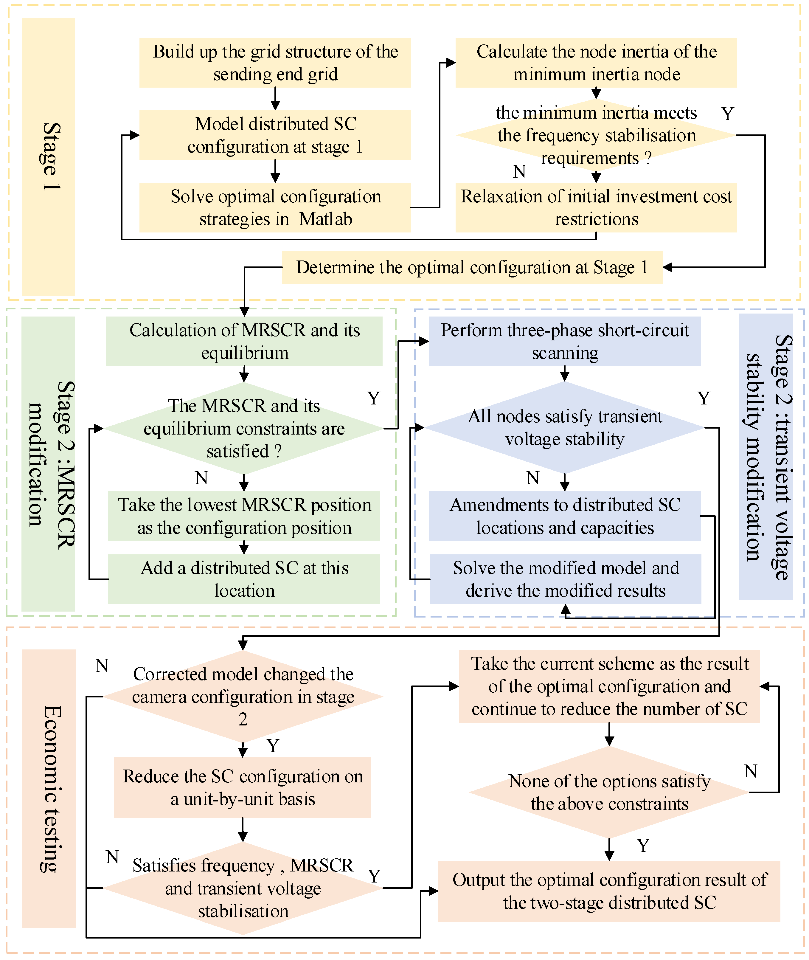
4.3. Solving Steps of the Two-Stage Optimal Configuration Strategy for Distributed SCs

For the transient simulation of the complex large-scale energy distribution system, the PSD-BPA simulation software (version 3.07) is selected for fault simulation. The Matlab particle swarm optimization algorithm is utilized to determine the optimal configuration of the distributed SCs. The solution process is illustrated in Figure 3.

(1)

Set the Matlab optimization initial parameters to set the initial values of the SC’s mounting position and capacity.

(2)

Stage 1 frequency stability optimization: optimize with the objective of maximizing the system inertia per unit of investment, derive the Stage 1 SC installation position and capacity results, and determine the minimum inertia to maintain frequency stability.

(3)

Stage 2 MRSCR calibration: check whether the Stage 1 optimization results satisfy the MRSCR and balancing constraints. If not, install additional SCs at the lowest MRSCR locations until the MRSCR machine balancing constraints are satisfied.

(4)

Stage 2 transient voltage calibration: Check the current configuration results against the transient voltage stability constraints. If the constraints are not met, make additional adjustments to the position and capacity of the SC until the constraints are met.

(5)

Economy check: If more SCs are installed in the second stage, the current configuration may be over-invested. The results in (4) are checked for economy, and if they are not satisfied, the SC configuration is gradually reduced until the constraints cannot be satisfied. The optimal configuration result will be chosen based on the maximum value of system inertia enhancement per unit of investment among all scenarios that satisfy each constraint.

(6)

Output the result of two-stage optimal configuration of distributed SC considering dynamic frequency support and transient voltage stability.

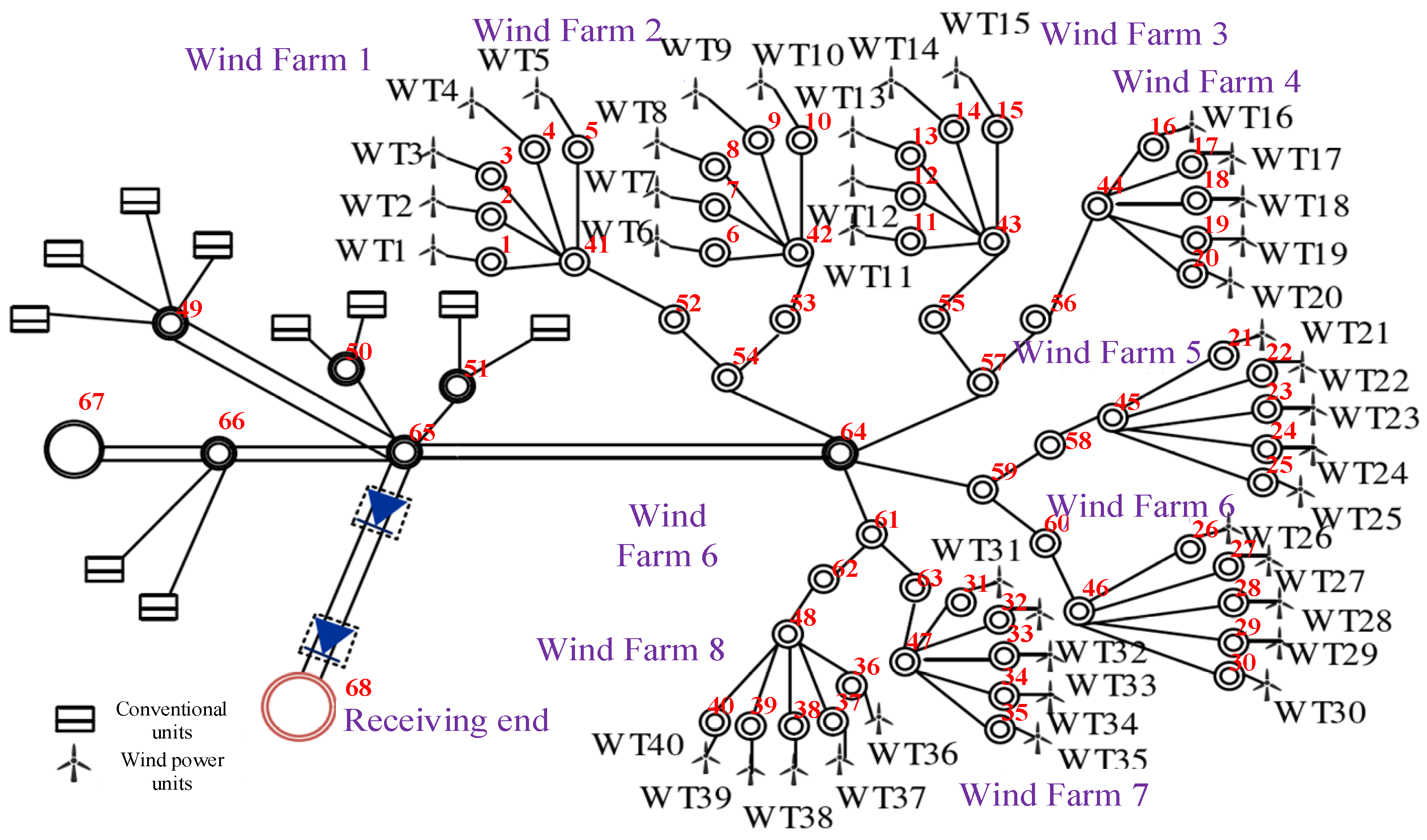
5. Case Study

5.1. Data Collection and Parameter Selection

The 68-node grid at the sending end of a large wind power generation base is the focus of this study, comprising eight large wind farms (total installed capacity of 4080 MW), 10 conventional energy power plants (total installed capacity of 4240 MW), and a set of UHV DC transmission lines (total outgoing power of 5500 MW). The network topology is illustrated in Figure 4.

Each node bus serves as the location for deploying the distributed SC, with its arrangement capacity being the variable to be optimized. The parameters for the particle swarm optimization algorithm are detailed in [24], while the parameters for the distributed SC are shown in

Table 1. SC parameters with a capacity of 50 MVar.

Parameter	Value	Parameter	Value
$\mathrm{Subtransient}\mathrm{reactance}{X}_d^{″}$	10.9 p.u.	Transient reactance X’d	16.1 p.u.
$\mathrm{Subtransient}\mathrm{time}\mathrm{constant}{T}_d^{″}$	0.06 s	Transient time constant T’d	7.47 s
Excitation system strong excitation multiplier	2.41	Stator non-periodic component time constant Ta	21.96 s

. Other parameters of case study are shown in

Table 2. Other parameters of the case study.

Parameter	Value	Parameter	Value
the unit-capacity SC cost of operation and maintenance Cm	0.2 million yuan	the upper limit of the distributed SC initial investment cost Cinv,max	0.8 billion yuan
the cost of purchasing and installing a single SC Cta,p	0.031 billion yuan	the maximum frequency deviation Δfdis-max	0.23 Hz
$\mathrm{the}\mathrm{minimum}\mathrm{critical}\mathrm{inertia}{H}_{RoCoF}^{\mathit{min}}$	2.55	the maximum change rate of frequency required by the national standard RoCoFmax	3 Hz/s
the upper limit of MRSCR equalization λMRSCR	1.5	the reference frequency fs	50 Hz
the upper number limit of accessing to the distributed SCs κp,max	4

.

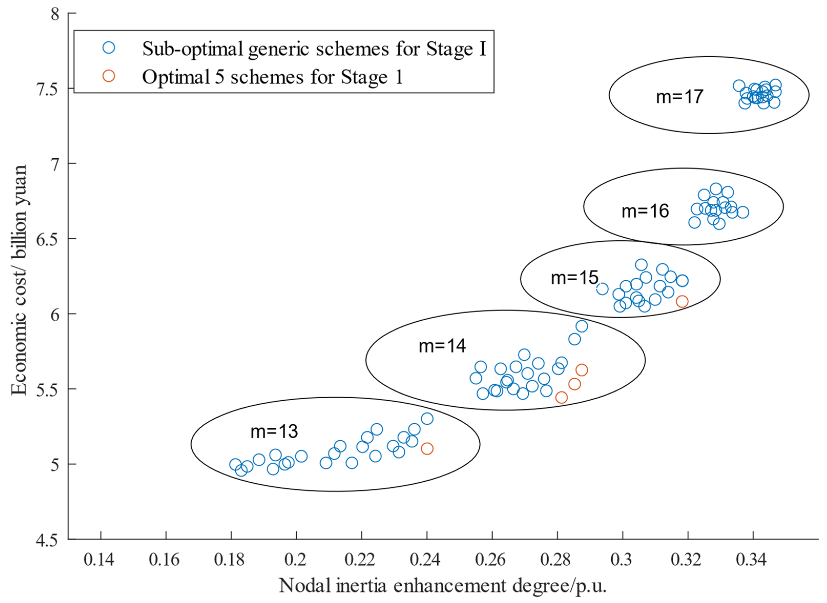
5.2. Stage 1: Distributed SC Configuration Results Considering Economic Cost and Dynamic Frequency Support

Based on the Matlab simulation results for calculating the objective function value of each configuration scheme in Stage 1, the coupling relationship between economic cost and node inertia enhancement is depicted in Figure 5. The optimal five schemes are marked with red markers.

As shown in Figure 5, since the capacity of each distributed SC is 50 MW, at least 13 SCs are needed to meet the frequency stability requirements of large energy bases. As the installed capacity of the SC increases, the economic cost rises linearly, but the increase in node inertia gradually slows down. It is unreasonable to blindly increase nodal inertia at a significant additional economic cost. Therefore, this strategy aims to achieve the maximum node inertia enhancement rate with minimal economic cost, balancing economic benefits and frequency stability. A comparison of the configuration results of the five schemes marked in red is shown in

Table 3. Configuration results for the optimal five scenarios.

Number	SC Access Location and Number	Total Accessed Number	Total Capacity Accessed (MVar)	Total Economic Cost (Billion Yuan)	Node Inertia Enhancement Degree	Objective Function Value F
Scheme 1	41(1),42(2),43(2),44(2),45(2),46(2),47(1),48(1)	13	650	0.528	0.24	0.0462
Scheme 2	41(2),42(2),43(2),44(2),45(1),46(2),47(2),48(1)	14	700	0.545	0.284	0.0521
Scheme 3	41(2),42(2),43(2),44(2),45(2),46(2),47(1),48(1)	14	700	0.565	0.287	0.0513
Scheme 4	41(2),42(2),43(2),44(2),45(1),46(2),47(1),48(2)	14	700	0.572	0.289	0.0507
Scheme 5	41(2),42(2),43(2),44(2),45(2),46(2),47(2),48(1)	15	750	0.615	0.316	0.0518

.

As shown in Table 3, the distributed SCs are installed at the bus of wind farms’ convergence station. This allows each wind turbine node to have the shortest electrical distance from the SCs. Scheme 2 achieves the largest system node inertia enhancement (0.284) at the least economic cost (528 million yuan). The node inertia enhancement per unit investment for Schemes 1 and 5 is less than that of Scheme 2 due to differences in the number of SCs accessed. Scheme 1 achieves frequency stabilization (0.24) with the least number of SC installations (13), but its inertia improvement per unit investment is insufficient. Because Scheme 5 is too large an investment, its inertia enhancement per unit investment is not as good as Scheme 2. The differences between Schemes 2, 3, and 4 are the varying locations of the distributed SCs on different wind power aggregation buses. Schemes 3 and 4 are not as economical as Scheme 2. Although Scheme 2 does not achieve the largest node inertia enhancement at the second SC of the 47th node, it has the lowest investment cost due to geographic factors, making Scheme 2 the optimal configuration for the first stage. The distribution of system node inertia before and after the SC configuration is visually analyzed in Figure 6.

The comparison in Figure 6 shows a significant improvement in node inertia before and after the distributed regulator configuration. Nodes with higher serial numbers have significantly smaller node inertia than those with lower serial numbers because high-inertia synchronous generator sets are numbered backward, while wind power plants without inertia support are numbered forward. Additionally, since Wind Farm 5 and Wind Farm 7 convergence stations each have only one SC in Scheme 2, the inertia enhancement of nodes 21–25 and 31–35 is not as good as other wind farm nodes. A comparison of the frequency response in the case of a three-phase short-circuit fault at the node with the lowest inertia is shown in Figure 7.

The orange curve represents the scheme without SC access, and it can be seen that its RoCoF is close to 15 Hz/s, which seriously exceeds the specified value of RoCoF. Comparing the orange and blue curves, it is evident that a large number of RE units reduce the system inertia level and weaken frequency modulation capability, posing a serious threat to system frequency safety. As shown by the yellow curve, RoCoF is about 4 Hz/s, and the frequency is reduced by 0.3 H. The system’s equivalent inertia time constant significantly increases after the SC configuration, meeting the requirements for maximum transient frequency deviation Δf_dis-max and maximum rate of change in frequency RoCoF_dis-max.

5.3. Stage 2: Installation Location and Capacity Modification Results for Distributed SC Considering Economic Cost and Dynamic Frequency Support

According to the short-circuit ratio requirements for RE stations at the sending end of large energy bases [25], the short-circuit ratio of each wind farm must exceed 1.5, the overall short-circuit ratio must surpass 12.5, and the maximum threshold for short-circuit ratio balance is 1.25. The MRSCR results of wind farms at the sending end of the grid, after the initial stage of SC configuration, have been corrected. A comparison of the distributed SCs is presented in

Table 4. Correction comparison before and after distributed SC configuration considering MRSCR improvement.

Wind Farm Number	MRSCR of Each Wind Farm before Correction	Overall Short Circuit Ratio and Balance before Correction	MRSCR of Each Wind Farm after Correction	Overall Short Circuit Ratio and Balance after Correction
Wind Farm 1	1.562	11.673 and 1.316	1.672	12.976 and 1.189
Wind Farm 2	1.368		1.611
Wind Farm 3	1.539		1.642
Wind Farm 4	1.528		1.635
Wind Farm 5	1.237		1.588
Wind Farm 6	1.512		1.645
Wind Farm 7	1.488		1.611
Wind Farm 8	1.439		1.572

before and after corrections, considering the enhancement of MRSCR.

Wind Farms 2, 5, 7, and 8 do not meet the short-circuit ratio requirement before correction. Their overall short-circuit ratio and equalization also fall short of the set criteria. According to the iterative process described in Section 4.2, the distributed regulator can be configured starting from the plant with the lowest MRSCR. By increasing the configuration of the distributed SC, the short-circuit ratio requirement of the delivery system can be met, as shown in

Table 5. Distributed SC correction process considering MRSCR improvement.

Configuration Times	Configuration of Wind Farms and Their Locations	Minimum Short Circuit Ratio before Correction	Minimum Short Circuit Ratio after Correction	Short Circuit Ratio Balance after Correction
1	Wind Farm 5 (45)	1.237	1.428	1.237
2	Wind Farm 2 (42)	1.428	1.572	1.189

.

After configuring a distributed SC on the converging station bus of Wind Farm 5 and Wind Farm 2, each wind farm meets the MRSCR requirements. The corrected overall short-circuit ratio is 12.976, which is greater than 12.5, and the MRSCR equilibrium degree is 1.189, which is less than 1.25, thus meeting the specified requirements.

To analyze the transient voltage stability of the wind farms, PSD-BPA software (version 3.07) is used to construct a large-scale energy base sending-end grid model, which conducts transient voltage stability analysis. Two fault cases are considered: a three-phase short circuit at 0.5 s on the high-voltage bus of each wind farm, and a failure in UHV DC commutation.

Due to the first and second stages of MRSCR enhancement already being configured for the distributed SCs, the three-phase short circuits did not cause transient low voltages or over voltages. However, under the UHV DC commutation failure condition, transient voltages at the machine terminals of Wind Farms 7 and 8 (nodes 31, 34, and 36) exceeded 1.3 p.u. for 0.5 s after the fault, and transient low voltages appear at node 31 of Wind Farm 7. According to the transient voltage stabilization constraints, a transient voltage stabilization correction is required for the distributed SC. After the Stage 2 capacity correction of the SC configuration based on transient voltage stability, the system transient voltage stability requirement is met by adding one SC at the machine ends of nodes 31 and 36, respectively. The voltage curves of nodes 31 and 36 before and after correction under DC commutation failure conditions are shown in Figure 8.

As shown in Figure 8, the peak value of 1.32 p.u. exceeds the specified maximum value, and the minimum value of 0.625 does not satisfy the transient voltage stabilization requirement without access to the SC at the machine end of nodes 31 and 36. The voltage of the orange curve exceeds the transient voltage stabilization requirement (red dashed line). However, the system transient voltage stabilization requirement can be satisfied by adding an SC at the machine end of nodes 31 and 36, respectively (blue line).

Since the number of SCs in Stage 2 has been increased, there is a possibility of over-investment in the current configuration. Thus, the SC configuration is gradually reduced until the constraints cannot be met. The final configuration, which maximizes system inertia improvement per unit of investment, is selected from all schemes that satisfy each constraint. The optimal configuration result is presented in Table 5, which involves reducing one SC at node 47 of the Wind Farm 7 convergence station compared to the scheme before economic calibration. This adjustment is necessary, as additional SCs are allocated at node 47 and machine end node 31 by the MRSCR and transient voltage stability correction models, resulting in an over-investment situation. By reducing one SC at node 47, the system constraints can still be met, while achieving the maximum improvement in unit investment system inertia.

As shown in

Table 6. Optimal configuration results of the two-stage distributed SCs after economic calibration.

SC Access Location and Number	41(2), 42(2), 43(2), 44(2), 45(2), 46(2), 47(2), 48(1), 31(1), 36(1)	Maximum Frequency Change Rate (Hz/s)	1.51
Total Access Capacity (MVar)	850	Sending-end grid overall MRSCR	14.251
Total economic cost (billion yuan)	0.751	Short circuit ratio balance	1.092
Nodal inertia enhancement degree	0.347	Maximum transient overvoltage (p.u.)	1.29
Maximum frequency deviation (Hz)	0.196	Minimum transient overvoltage (p.u.)	0.77

, the two-stage distributed SCs considering dynamic frequency support and transient voltage stabilization is configured with a total of 17 units of 850 MVar. Seventeen distributed SCs (at a cost of 0.751 billion yuan) are installed at the large wind power generation base, which can more accurately control the voltage, frequency, and other parameters in the power system, improve the efficiency of energy utilization, and reduce energy waste. In addition, access to the SCs can quickly respond to changes in the power system, improve the response speed and flexibility of the system, help to cope with sudden load fluctuations, and improve the stability of system operation. At this time, all wind farms satisfy the MRSCR and transient voltage stabilization requirements and have the largest system inertia enhancement per unit investment. The corrected sending-end grid overall MRSCR is 14.251. The short-circuit ratio balance is 1.092, and the maximum and minimum transient voltages under the worst fault (1.29, 0.77 p.u.) meet the given requirements.

5.4. Sensitivity Analysis of SC Capacity Configurations to DC Reactive Power Demand and Transient Voltage

To analyze the sensitivity of different SC capacity configurations to varying DC reactive power demands and transient voltages, Wind Farm 2 (42) and Wind Farm 5 (45) are taken as examples. A UHV commutation failure case is set up to simulate and verify the SC configurations with different capacities. The transient voltage waveforms are depicted in Figure 9.

The voltage curves of one and two SCs connected at node 42 are similar, both returning to the pre-fault voltage level. However, a single SC exhibits weak reactive power support capacity, taking a longer time to reach the standard bus voltage and failing to meet the transient voltage requirements. The waveform of single SC at node 45 only slightly outperforms the scheme without SC configuration. This indicates that single distributed SC at node 42 fails to meet the transient voltage requirements, whereas accessing two SCs after the system transient voltage can meet the set requirements. The transient voltage waveforms reveal a significant reactive power deficit in the DC system during the sub-transient and transient processes, continuing to consume reactive power post-fault removal, as shown in Figure 10.

It is observed that in the absence of SC accessing, the reactive power demand cannot be met due to continuous DC commutation failure. Accessing single SCs, despite achieving nearly 2.3 times the reactive power output through strong excitation, still fails to meet the converter’s reactive power consumption, ultimately causing the bus voltage to drop below the critical level. Upon accessing two SCs, strong excitation reaches 3.9 times the reactive power output to fulfill the converter’s reactive power consumption (3.7 times the rated capacity).

6. Discussion and Future Work

6.1. Discussion

The proposed model is validated using the feeder grid of a large energy base in western China. The results demonstrate that the optimal configuration scheme effectively suppresses transient overvoltage at the generator end and significantly enhances the system’s dynamic frequency support strength. The following conclusions can be drawn from the analysis of the results:

(1)

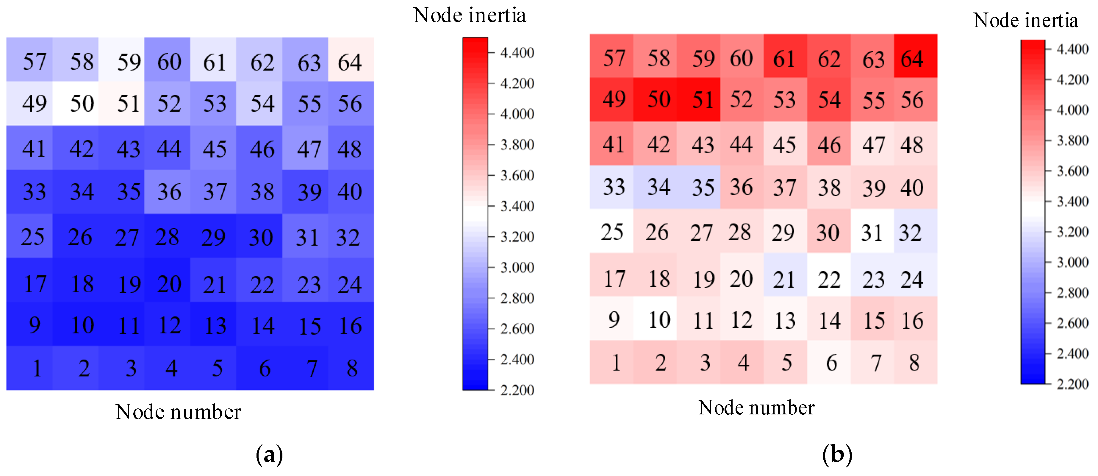
Nodal inertia can reflect the distribution characteristics of system inertia and can be utilized to identify weak points in dynamic frequency support. By considering the critical inertia for frequency stability, distributed SCs can be installed at the bus with the lowest nodal inertia at the convergence station, effectively enhancing dynamic frequency support. Therefore, this strategy aims to achieve the maximum node inertia enhancement rate (0.347) with minimal economic cost (0.751 billion yuan), balancing economic benefits and frequency stability.

(2)

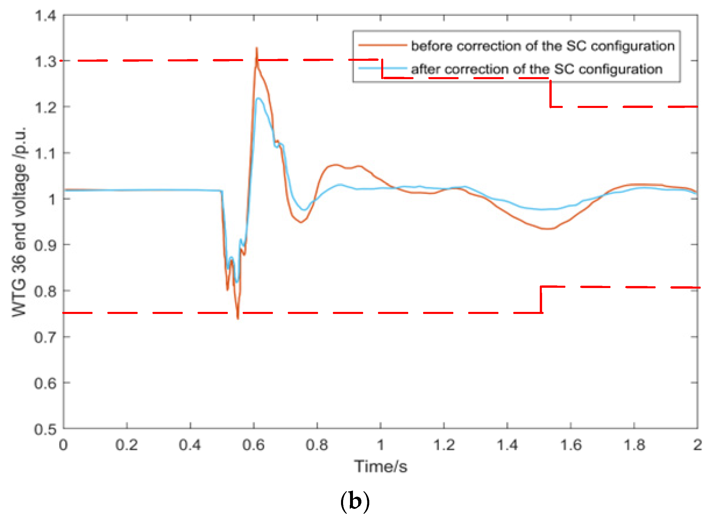
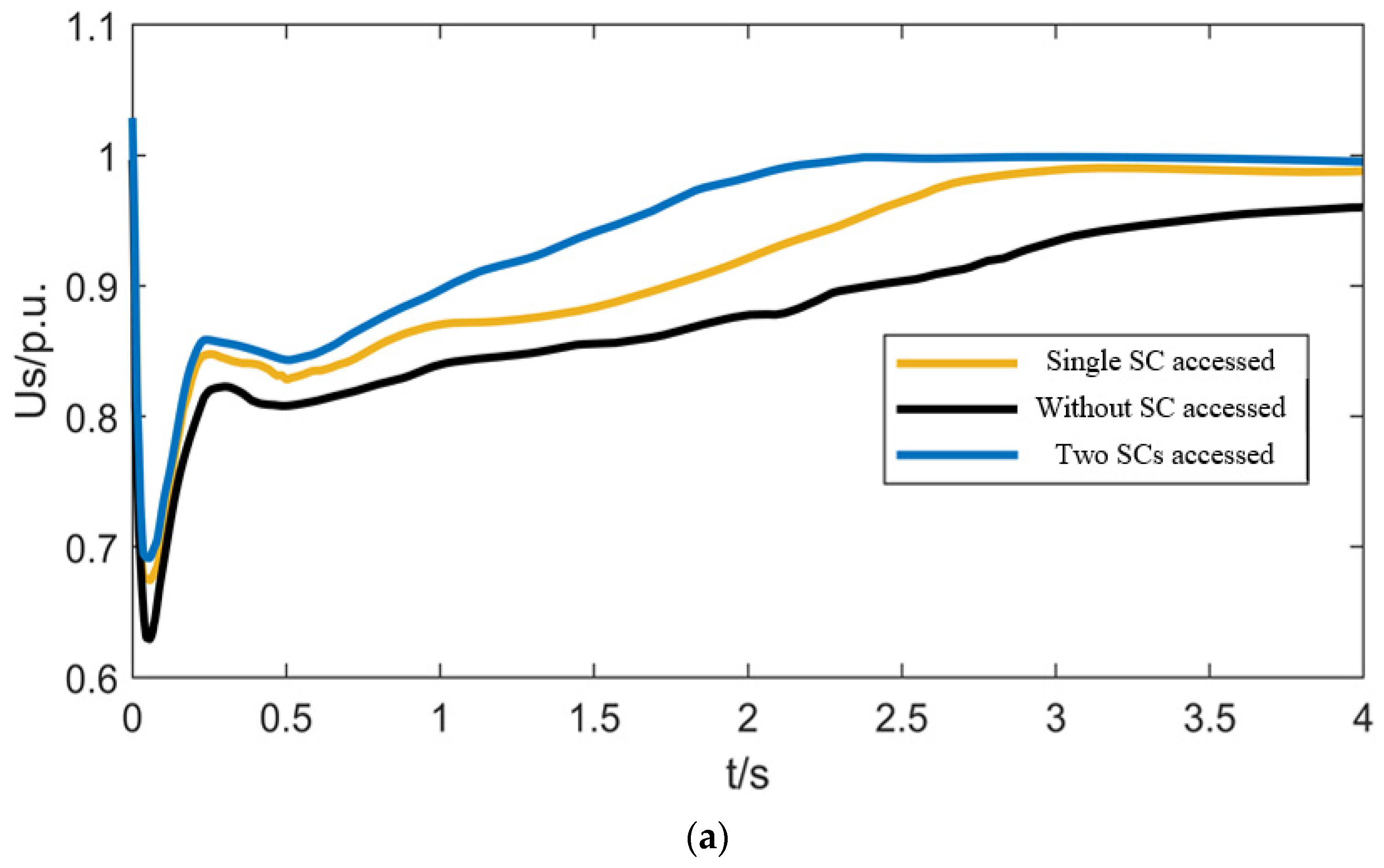
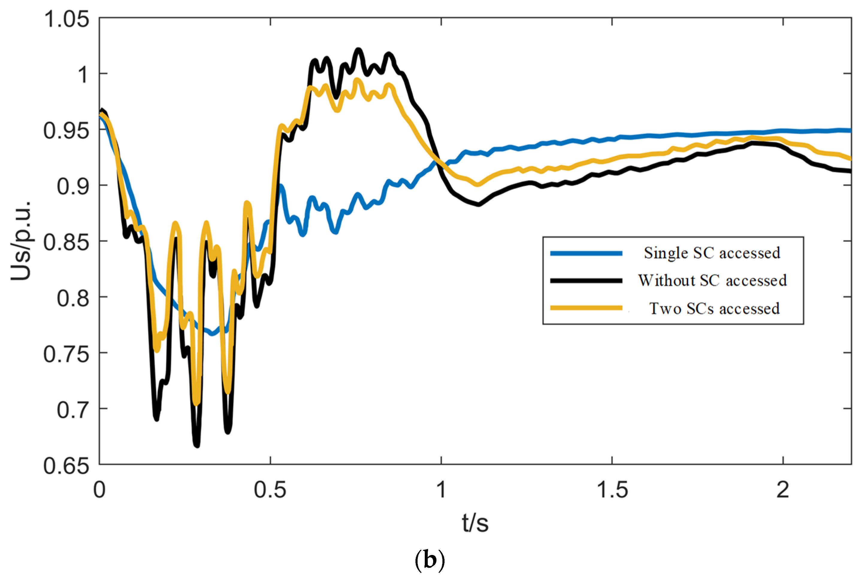
The MRSCR analysis of the RE convergence area demonstrates the enhancement of MRSCR for wind farms. This strategy elucidates the impact mechanism of the SC transient reactive power characteristics during the sub-transient and transient processes in the sending-end grid. A specific case study confirms that the installation of distributed regulating equipment in the sending-end grid successfully mitigates transient overvoltage at the machine end, significantly enhancing transient voltage support. Upon accessing two SCs at node 45, strong excitation reaches 3.9 times the reactive power output to fulfill the converter’s reactive power consumption (3.7 times the rated capacity).

(3)

By considering the location and capacity of the SCs as variables, a two-stage optimal configuration strategy of distributed SCs is proposed at the sending end of large-scale wind power generation bases, considering dynamic frequency support and transient voltage stabilization. The results indicate that the optimized configuration, while meeting MRSCR, equilibrium, and transient voltage stability constraints, maximizes system inertia enhancement per unit of investment and avoids over-investment. This optimal configuration model addresses the improvement of dynamic frequency response, filling a current gap in end-of-send distributed regulator configurations that do not consider dynamic frequency support enhancements.

6.2. Limitations and Future Work

Currently, the configuration of reactive power compensation for UHV DC sending-end grid in China is still undergoing continuous development and improvement. However, existing strategies have certain limitations, and future research can address the following areas.

(1)

Future studies can enhance modeling methods. For example, incorporating novel energy storage systems [26] and user-side behavior [27] into the operational model can extend its applicability to various scenarios.

(2)

The scope of the research in this thesis can be further expanded with more detailed data support. The model can be simulated on a monthly, yearly, or multi-year basis to investigate the optimal operational modes for large-scale energy base reactive power compensation configurations over long-term periods.

(3)

Since distributed capacitors can also improve the transient voltage characteristics, we will further study the synergistic planning of distributed capacitors with distributed SCs. In addition, we will study the relationship between the frequency variation in the center of inertia and the inertia of the system, and the disturbed power under various faults using the neural network model [28].

References

1. Chen, G.; Dong, Y.; Liang, Z. Analysis and reflection on high-quality development of new energy with Chinese characteristics in energy transition. Proc. CSEE 2020, 40, 5493–5505. (In Chinese) [Google Scholar]
2. Klyuev, R.; Bosikov, I.; Gavrina, O. Use of Wind Power Stations for Energy Supply to Consumers in Mountain Territories. In Proceedings of the 2019 International Ural Conference on Electrical Power Engineering (Uralcon), Chelyabinsk, Russia, 3–1 October 2019; pp. 116–121. [Google Scholar]
3. Cheng, X.; Yan, B.; Zhou, X.; Yang, Q.; Huang, G.; Su, Y.; Yang, W.; Jiang, Y. Wind resource assessment at mountainous wind farm: Fusion of RANS and vertical multi-point on-site measured wind field data. Appl. Energy 2024, 363, 123116. [Google Scholar] [CrossRef]
4. Shen, G.; Xin, H.; Liu, X.; Tu, J.; Wang, K.; Wang, N. Analysis on synchronization instability mechanism and influence factors for condenser in large-scale renewable energy base. Autom. Electr. Power Syst. 2022, 46, 100–108. (In Chinese) [Google Scholar]
5. Zhang, X.; Liu, F.; Wang, S. Measures to enhance new energy consumption in extra-high voltage direct current feeder grids. Proc. CSU-EPSA 2022, 34, 135–141. [Google Scholar]
6. Jin, Y.; Yu, Z.; Li, M.; Jiang, W. Comparison of new generation regulator and power electronic reactive power compensation device applied in extra-high voltage AC and DC grids. Power Grid Technol. 2018, 42, 2095–2102. [Google Scholar]
7. Cao, W.; Zhang, T.; Fu, Y.; Yao, Y.B.; Chen, S.Y. Research and application of synchronous regulator to enhance power system inertia and improve frequency response. Power Syst. Autom. 2020, 44, 1–10. [Google Scholar]
8. Mansour, M.Z.; Me, S.P.; Hadavi, S.; Badrzadeh, B.; Karimi, A.; Bahrani, B. Nonlinear transient stability analysis of phased-locked loop-based grid-following voltage-source converters using Lyapunov’s direct method. IEEE J. Emerg. Sel. Top. Power Electron. 2022, 10, 2699–2709. [Google Scholar] [CrossRef]
9. He, X.; Geng, H. Transient stability of power systems integrated with inverter-based generation. IEEE Trans. Power Syst. 2021, 36, 553–556. [Google Scholar] [CrossRef]
10. Li, W.; Qian, Z.; Wang, Q.; Wang, Y.; Liu, F.; Zhu, L.; Cheng, S. Transient voltage control of sending-end wind farm using asynchronous condenser under commutation failure of HVDC transmission system. IEEE Access 2021, 9, 54900–54911. [Google Scholar] [CrossRef]
11. Suo, Z.; Liu, J.; Jiang, W.; Li, Z.; Yang, L. Research on the configuration of regulator for large-scale new energy DC transmission system. Electr. Power Autom. Equip. 2019, 39, 124–129. [Google Scholar]
12. Chang, H.; Huo, C.; Liu, F.; Liu, F.; Ke, X.; Hou, Y.; Niu, S.; Wang, C. Research on optimal configuration of regulating camera for improving transient voltage stability level of weak feeder grid. Power Syst. Prot. Control 2019, 47, 90–95. [Google Scholar]
13. Yang, J.; Shi, Z.; He, C.; Li, X.; Liang, Y. Optimal configuration strategy of condenser for improving short-term voltage safety in a sending-end power grid with a high renewable penetration level. J. Shandong Univ. 2024, 54, 174–182. [Google Scholar]
14. Wang, Z.; Liu, M.; Li, H.; Qin, J.; Guo, J.; Bai, K. Optimal allocation method of regulating camera to enhance new energy cluster delivery capacity of weak grid. Electr. Power Autom. Equip. 2024, 1–10. [Google Scholar] [CrossRef]
15. Wang, Q.; Li, T.; Tang, X.; Liu, F.; Lei, J.; Yuan, C. Method of site selection for synchronous condenser responding to commutation failures of multi-infeed DC system. Autom. Electr. Power Syst. 2019, 43, 222–227. (In Chinese) [Google Scholar]
16. Zhou, Y.; Sun, H.; Xu, S.; Wang, X.; Zhao, B.; Zhu, Y. Synchronous condenser optimized configuration scheme for power grid voltage strength improvement. Power Syst. Technol. 2022, 46, 3848–3856. (In Chinese) [Google Scholar]
17. Guo, Q.; Li, Z. A review on the development of synchronous regulator. Proc. CSEE 2023, 43, 6050–6064. [Google Scholar]
18. Gao, H.; Yuan, H.; Xin, H.; Huang, L.; Feng, C. Nodal frequency performance of power networks. In Proceedings of the IEEE 8th International Conference on Advanced Power System Automation and Protection, Xi’an, China, 21–24 October 2019; pp. 1838–1842. [Google Scholar]
19. Zhang, Z.; Zhou, M.; Wu, Z.; Liu, J.; Liu, S.; Guo, Z. An energy storage siting and capacity planning method considering dynamic frequency support. Proc. CSEE 2023, 43, 2708–2721. [Google Scholar]
20. Liu, F.; Xu, G.; Liu, J.; Wang, C.; Bi, T.; Guo, X. Characteristics of power system inertia distribution considering grid structure and parameters. Autom. Electr. Power Syst. 2021, 45, 60–67. [Google Scholar]
21. Wang, B.; Sun, H.; Li, W.; Yan, J.; Yu, Z.; Yang, C. Minimum inertia assessment of power systems considering dynamic frequency constraints. Proc. CSEE 2022, 42, 114–127. [Google Scholar]
22. Li, S.; Tian, B.; Li, H.; Luo, Y.; Huang, S.; Xu, S. A time-phased method for limiting wind power output based on frequency security constraint and critical inertia calculation. Power Syst. Prot. Control 2022, 50, 60–71. [Google Scholar]
23. Zheng, C.; Sun, H.; Yang, D. Transient voltage instability criterion and control based on wide-area branch response. Proc. CSEE 2023, 43, 9470–9481. [Google Scholar]
24. Zhang, Y.; Xu, Y.; Zhang, R.; Dong, Z.Y. A missing-data tolerant method for data-driven short-term voltage stability assessment of power systems. IEEE Trans. Smart Grid 2019, 10, 5663–5674. [Google Scholar] [CrossRef]
25. Xiao, H.; Sun, K.; Pan, J.; Li, Y.; Liu, Y. Review of hybrid HVDC systems combining line communicated converter and voltage source converter. Int. J. Electr. Power Energy Syst. 2021, 129, 106713. [Google Scholar] [CrossRef]
26. Sun, H.; Xu, S.; Xu, T.; Guo, Q.; He, J.; Zhao, B.; Yu, L.; Zhang, Y.; Li, W.; Zhou, Y.; et al. Definition and index of short circuit ratio for multiple renewable energy stations. Proc. CSEE 2021, 41, 497–505. (In Chinese) [Google Scholar]
27. Huang, W.; Zhang, B.; Ge, L.; He, J.; Liao, W.; Ma, P. Day-ahead optimal scheduling strategy for electrolytic water to hydrogen production in zero-carbon parks type microgrid for optimal utilization of electrolyzer. Energy Storage 2023, 68, 107653. [Google Scholar] [CrossRef]
28. Ahmad, M.S.; Ali, M.S.; Abd, R.N. Hydrogen energy vision 2060: Hydrogen as energy carrier in Malaysian primary energy mix—Developing P2G case. Energy Strategy Rev. 2023, 35, 100632. [Google Scholar] [CrossRef]
Figure 1. Sending-end equivalent network of large energy base convergence area.
Energies 17 04748 g001
Figure 2. Simplified AC equivalent circuit after condenser access.
Energies 17 04748 g002
Figure 3. Solving process for the two-stage optimal configuration model of distributed SCs in Matlab software (version 2021a).
Energies 17 04748 g003
Figure 4. Wiring diagram for sending-end grid of large energy bases in China.
Energies 17 04748 g004
Figure 5. Coupling relationship between economic cost and node inertia enhancement.
Energies 17 04748 g005
Figure 6. Comparison of node inertia improvement before and after distributed regulator configuration. (a) Before the distributed SC configuration. (b) After the distributed SC configuration.
Energies 17 04748 g006
Figure 7. Frequency comparison before and after distributed SC configuration.
Energies 17 04748 g007
Figure 8. Voltage curves of nodes 31 and 36 before and after correction of the distributed SC. (a) The voltage curves of node31 before and after correction of the distributed SC. (b) The voltage curves of node36 before and after correction of the distributed SC.
Energies 17 04748 g008aEnergies 17 04748 g008b
Figure 9. Comparison of 42 and 45 transient voltage waveforms. (a) Transient voltage waveform at node 42. (b) Transient voltage waveform at node 45.
Energies 17 04748 g009aEnergies 17 04748 g009b
Figure 10. DC system reactive power output and demand.
Energies 17 04748 g010