Article

Impact of Data Corruption and Operating Temperature on Performance of Model-Based SoC Estimation

by
King Hang Wu
1,*,
Mehdi Seyedmahmoudian
1,
Saad Mekhilef
1,2,
Prashant Shrivastava
2 and
Alex Stojcevski
3
1
School of Science, Computing and Engineering Technologies, Swinburne University of Technology, Hawthorn, Melbourne, VIC 3122, Australia
2
Power Electronics and Renewable Energy Research Laboratory (PEARL), Department of Electrical Engineering, University of Malaya, Kuala Lumpur 50603, Malaysia
3
PVC and President, Curtin University, Singapore 117684, Singapore
*
Author to whom correspondence should be addressed.
Energies 2024, 17(19), 4791; https://doi.org/10.3390/en17194791
Submission received: 9 May 2024 / Revised: 17 September 2024 / Accepted: 19 September 2024 / Published: 25 September 2024

Abstract

:
Electric vehicles (EVs) are becoming popular around the world. Making a lithium battery (LIB) pack with a robust battery management system (BMS) for an EV to operate under different complex environments is both a challenge and a requirement for engineers. A BMS can intelligently manage LIB systems by estimating the battery state of charge (SoC). Due to the nonlinear characteristics of LIB, influenced by factors such as the harsh environment and data corruption caused by electromagnetic interference (EMI) inside electric vehicles, SoC estimation should consider available capacity, model parameters, operating temperature and reductions in data sampling time. The widely used model-based algorithms, such as the extended Kalman filter (EKF) have limitations. Therefore, a detailed review of the balance between temperature, data sampling time, and different model-based algorithms is necessary. Firstly, a state of charge—open-circuit voltage (SoC-OCV) curve of LIB is obtained by the polynomial curve fitting (PCF) method. Secondly, a first-order RC (1-RC) equivalent circuit model (ECM) is applied to identify the battery parameters using a forgetting factor-based recursive least squares algorithm (FF-RLS), ensuring accurate internal battery parameters for the next step of SoC estimation. Thirdly, different model-based algorithms are utilized to estimate the SoC of LIB under various operating temperatures and data sampling times. Finally, the experimental data by dynamic stress test (DST) is collected at temperatures of 10 °C, 25 °C, and 40 °C, respectively, to verify and analyze the impact of operating temperature and data sampling time to provide a practical reference for the SoC estimation.

1. Introduction

The EV growth in the market is dramatic, as some significant countries have set a timeline for transitioning transportation from diesel/petrol vehicles to electric vehicles. China has committed to achieving carbon neutrality by 2060, and EVs will become one of the strategic industries that will help China achieve its climate goals [1]. In the UK, the full transition to electric vehicles (EVs) will be one of the most important steps in achieving the Net Zero target. By 2032 at the latest, the Climate Change Committee (CCC) has called for all new light-duty vehicles sold to be fully battery-electric, including passenger vehicles, taxis, vans, motorbikes, and mopeds. In order to reach Net Zero, all vehicles must be fossil fuel-free by 2050. It included the heavy-goods vehicles (HGVs) [2]. Therefore, a BMS equipped with an intelligent algorithm for accurately estimating the SoC of the battery is very important to ensure the safety of the EV system.
The performance of a new generation EV has been improved significantly. The capacity of an EV’s LIB is powerful enough for traveling long distances on a continent. Therefore, EV applications require a very high capacity battery. Considering the high battery capacity, a super-fast EV charger is necessary to satisfy the short EV charging time requirement. Pantograph is one of the hyperchargers that can support up to 600 kW for EV battery charging. It significantly shortens the EV battery charging time. However, plenty of heat would be generated during the charging process because the output charging current of the Pantograph is very high. Some crucial components also generate heat to raise the battery’s temperature: manual service disconnect (MSD), high power socket, copper bus bar, internal space of the battery pack, heat radiation design, and cell balancer. It causes the battery’s acute internal chemical reaction to radiate too much heat. In real applications, EVs always operate at different temperature environments. The temperature variation is very different in one day. At least 10 °C difference between day and night is common in some countries. Because LIB is sensitive to temperature variation, the accuracy of SoC estimation would be influenced; different internal and external factors, such as operating temperatures, charging/discharging processes, and internal resistance, profoundly cause various severe levels of estimation error. It would shorten the battery lifespan and cause safety hazards such as fire or explosion. Thus, researchers developed robust algorithms to tackle these problems during the SoC estimation.
Thus, researchers proposed a complicated mathematical calculation to implement a thermal battery model to estimate the temperature effect generated during the LIB charging and discharging process. The paper [3,4,5] proposed an online method to generate the parameters through a thermal battery model. However, it causes a hefty computational load on the EV system, and the cost of hardware platforms must be increased. In paper [6], researchers proposed building a thermal battery model using the LIB’s internal heat. However, engineers can only stick the temperature sensor to the surface of the battery. Therefore, it is not easy to measure the battery’s internal temperature. As a result, the thermal model may not reflect SoC’s accuracy due to the lack of precision measurement of the temperature sensor. In paper [7], researchers proposed that measuring the surface temperature is good enough because there is a rising time difference between the surface and the center of the battery. Paper [8] shows that there is an important relationship between the ambient temperature and battery parameters. Paper [9] talks about internal resistance, an important factor for the thermal modeling of LIBs. This paper’s review series of experiments reflects the clear relationship between operating temperature and battery parameters for SoC estimation. Using the FF-RLS algorithm [10], an iterative calculation can identify updated internal battery parameters from the 1-RC ECM. The characteristics of the battery parameters will be analyzed deeply. The relationship between battery parameters and operating temperature will be discussed to show how it can be utilized for SoC estimation.
Electric vehicles need modernized electronic devices and energy controls integrated into electric vehicles to support intelligent autonomous operation. Even though the innovative electronic systems increase the comfort of driving these electric vehicles, they also increase the sensitivity to EMI [11]. Electronic systems act as both sources and targets of electromagnetic emissions. Both signal and power systems in a relatively small space of electric vehicles make the system even worse, with increased emissions and sensitivity. The EMI creates a harsh environment for onboard electronic devices to function appropriately inside an electric vehicle. Electric motors, power converters, high-power cable harnesses, traction batteries, interconnectors, and battery chargers are usually the main sources of EMI generated inside an electric vehicle.
For internal sources, a power converter is a main source of EMI to interfere with the electric driving systems; these systems require high-speed switching devices to work at frequencies up to a few ten kilohertz. The current flow in the traction battery, cable, and interconnector are part of the sources of electric and magnetic field (EMF) emission that creates a path for EMI. High-power cables carry a high level of current between the electric motor and the battery pack of an EV and generate stronger electromagnetic fields. High-voltage and low-voltage cables are placed nearby due to limited space for wiring, causing severe EMI between them.
For external sources, the battery charger and the wireless battery charger are the main external EMI sources; transferring power to the EV by connecting to a wireless charger creates a very powerful electromagnetic field. The three-phase alternative current (AC) to direct current (DC) converter and the onboard charger can also generate a very powerful EMI for the EV.
Nowadays, EV battery pack technology has improved a lot. A high-power battery pack would create a powerful EMI while transferring power to the EV through a high-power cable. EMI would severely corrupt the battery data transmission on the control area network (CAN) bus between the battery pack, vehicle control unit (VCU), and BMS [12,13]. Even though the CAN bus has a strong anti-interference ability, it is not difficult to discover data corruption in the firmware under the debug mode. Meanwhile, intermittent data loss is similar to a decrease in the data sampling time. The deterioration severely diminishes the accuracy of SoC estimation. Details of analysis by experiment will be discussed in other sections.
Several methods are widely used for the SoC estimation of batteries, including current integration, voltage-based, model-based, and Date-driven methods.
The Coulomb Counting Method (CCM) [14,15,16] is a current integration method. CCM measures the current flowing of the battery and integrates the current value over time to calculate the total number of charges inside the battery. This method is simple and inexpensive. However, it can be prone to errors due to the wrong initial SoC value, battery aging, and temperature variations.
Open-circuit voltage Method (OCVM) [16,17,18] is a voltage-based method. This method measures the battery’s voltage at rest when not charging or discharging. Thus, the OCVM is only suitable for offline SoC estimation. Moreover, the relationship between open-circuit voltage (OCV) and SoC is nonlinear. SoC for LifePO4 (LFP) batteries is very challenging because the OCV curve of LFP batteries is very flat and very sensitive to noise. Furthermore, the OCVM is prone to errors due to temperature and other factors.
The model-based method (MBM) [19] uses mathematical models of the battery to estimate its SoC. These methods can be more accurate than voltage-based and current integration methods if the battery model parameters are accurate. However, precise battery parameters and characteristics are difficult to obtain online. Moreover, the ambient temperature and battery aging can easily affect the battery model’s accuracy. Thus, the accurate battery model can be complex to develop because a lot of computational power is required compared to other methods.
Researchers also consider using a Joint or Co-estimation method to estimate the battery SoC. The paper [20,21,22] proposed using the SoX method to acquire a very accurate SoC result. Researchers considered various factors for the estimation process to achieve a high-accuracy SoC result.
Extended Kalman filter (EKF) [23] is one of the model-based methods combining measurements from various sensors, such as current, voltage sensors, and battery model parameters, to estimate the SoC of a LIB. EKF is used in many nonlinear applications, including control systems, navigation systems, and robotics control, especially for the SoC estimation of LIB. EKF estimates the battery SoC by combining prediction and step update. However, EKF requires a lot of computational power, and the implementation is complex. Furthermore, if the initial state estimation is too far from the actual state, EKF may not quickly converge to a state solution. Despite this drawback, EKF is still a powerful method for battery SoC estimation to provide accurate results.
The mixed method (MM) is proposed in [16] to exploit the CCM and MBM. It is a straightforward, closed-loop method for SoC estimation. CCM is the engine that estimates the SoC value of LIBs. A closed-loop control system (CLCS) would provide a rectified voltage error factor to increase the accuracy of the SoC value. However, MM can only enhance the accuracy of SoC estimation after certain specific data sampling cycles. The response time is slower than that of CCM. Due to the unstable measured current data, MM cannot usually rapidly represent the accurate SoC result. Therefore, an improved coulomb counting method with an adaptive error correction (ICC-AEC) algorithm and a dual closed-loop control system (DCLCS) has been proposed [24] to address the issue of the existing MM. It can improve the error correction time of the existing CLCS method. Moreover, the AEC mechanism helps improve the accuracy of the online SoC estimation. A combination of the above methods is usually used for SoC estimation, depending on the specific application’s requirements. CCM and OCVM can be used for simple applications without highly accurate SoC estimation requirements. MBM, Joint methods, and EKF can be used for more complex applications requiring highly accurate SoC estimation.

1.1. Contributions

For EV applications, the accuracy of battery SoC estimation is essential in optimizing the LIBs’ performance. This paper carried out research to illustrate how BMS can generate an accurate SoC estimation under extreme temperatures and different data sampling times. The main contribution of this work involves three aspects as follows:
(a)
Analyzed the impact of complex temperature environments on the performance of model-based SOC estimation to prove that the battery parameters can support estimating the SoC accurately.
(b)
Analyzed the impact of different data sampling times on the performance of model-based SOC estimation methods such as CLCS, DCLCS, and EKF. The experiments show how various data sampling times, used to simulate the adverse effect of data corruption inside EVs, significantly affect the SoC estimation accuracy. The experiments also show which method is suitable for accurately estimating the SoC of the data corruption.
(c)
Analyzed the SoC estimation results at different temperatures, 10 °C, 25 °C, and 40 °C, which are validated under a dynamic load profile, and analyzed the performance of different model-based methods at different data sampling times to demonstrate that an automatic data sampling time correction is necessary for the EV system.

1.2. Paper Structure

The structure of this paper is described as follows: The concept and technique of model-based SoC estimation are discussed in Section 2. The SoC estimation by using different model-based methods is depicted in Section 3. The experimental setup and considered evaluation matrices are shown in Section 4. The performance of model-based methods for SoC estimation in terms of temperature and data sampling time is validated and discussed under the considered dynamic operating conditions in Section 5, and the conclusion and recommendations for future innovation development are discussed and explained in Section 6.

2. Model-Based SoC Estimation Methods

2.1. 1-RC Battery Modelling

The electrochemical reactions inside the battery are complicated and easily influenced by many external factors. Therefore, extensive research on battery mathematical model development is considered essential. Moreover, it has continuously been crucial yet difficult in industry and academia. Reliable battery state estimation algorithms are designed to more accurately describe batteries’ external characteristics, and a more cutting-edge BMS has been developed for new electric vehicles. Accurate modelling is necessary for this process. This chapter systematically introduces the characteristics and parameter identification of the equivalent circuit models.
The 1-RC battery model [25,26] is a simple equivalent circuit model amalgamation of a series resistor and capacitor. The battery can be modelled as a terminal voltage ( V t  in series with an ohmic resistance ( R 0 ), and a parallel-connected RC branch ( R 1  and  C 1 ), which is equivalent to the battery cell’s open-circuit voltage ( V O C V ).  V 1  is the voltage drop caused by the RC branch connected in parallel. The model does not accurately capture the complex behaviour of batteries, but it is relatively simple and easy to use. It can reduce the computational cost during the SoC estimation process. Therefore, the 1-RC model [27] is applied in this paper.
Figure 1 describes the electrochemical processes of the 1-RC battery model. The symbol I stands for the charging and discharging current of the battery. While charging or discharging electric vehicles, discharging current is usually defined as a positive value. Charging current is defined as a negative value. Equation (1) uses Kirchhoff’s voltage law to express the voltage of a battery model.
{ V ˙ 1 = V 1 R 1 C 1 1 C 1 I V t = V O C V V 1 I R 0
The 1-RC battery model describes the voltage response through ideal electrical components. A constant voltage source displays the static voltage characteristics, and the dynamic voltage characteristics, such as polarization and hysteresis, are described by parallel RC branches. These models are widely applied to battery SoC estimation of BMS and energy management systems for the advantages of small calculations and excellent real-time performance.
FF-RLS [28] is a recursive algorithm for estimating LIB parameters such as internal resistance ( R 0  and  R 1 ), capacitance ( C 1 ), and OCV. FF-RLS can adapt to behavior changes in LIBs over time. Therefore, FF-RLS is specifically helpful for online battery parameter estimation. First, the forgetting factor determines the gain value to estimate the latest LIB parameters. The gain value is adjusted in real-time according to the changing characteristics of the battery. Finally, FF-RLS uses an updated gain value to determine the present battery parameters based on the past estimated value online. Figure 2 shows the flow chart of the FF-RLS algorithm in detail.
The following equation is the mathematical calculation of the FF-RSL algorithm.
{ θ ( k ) = θ ( k 1 ) + ( k o ( k ) ( U t ( t ) φ ( k ) θ ( k 1 ) T ) ) T k o ( k ) = P ( k ) φ ( k ) T ( φ ( k ) P ( k ) φ ( k ) T + u ) P ( k + 1 ) = [ I K ( k ) φ ( k ) ] P ( k ) u
Equation (2), the system parameters and data vectors are  θ ( k )   and   φ ( k ) . λ is the component of the forgetting factor. The value range of λ falls between 0.9 and 1. In this research, the value of λ is presumed to be 0.97.
The recursive equation in discrete time form may be stated as follows when utilizing (2):
V t , k = ( 1 a 1 ) U o C k + a 1 V t , k 1 + a 2 I k + a 3 I k 1
The discrete-time form (3) can be rewritten as:
V t , k = θ K T φ K
where the matrix form of  θ ( k )   and   φ ( k )  are as follows,
θ k = [ ( 1 a 1 ) U o C k         a 1           a 2         a 3 ]
φ k = [ 1         U t ( t 1 )         I ( t )           I ( t 1 ) ]
Ultimately, the battery model parameters can be identified by the matrix expression as follows:
[ R s R t C t ] = [ a 2 ( ( a 3 ) ( a 1 ) ( a 2 ) ) / ( 1 + ( a 1 ) ) T s / ( ( a 3 ) ( a 1 ) ( a 2 ) ) ]

2.2. The OCV and SoC Relationship

The polynomial curve fitting [29] method efficiently constructs a mathematical model to present the OCV curve. The polynomial equation can best fit a series of changeable battery data. A single equation can present an entire battery’s OCV characteristic. The order of the polynomial determines the complexity of the polynomial function used to fit the data. The trade-off between accuracy and anti-noise capability can be adjusted by choosing different polynomial orders in the equation. Higher-order polynomials can provide a more accurate curve fit to the complex data, but the function may easily capture the noise. On the contrary, lower-order polynomials may not be able to capture the critical features of the complex data patterns but with a more robust anti-noise capability. Equation (8) shows a 5th-degree order polynomial equation used to present the battery OCV model.
O C V P o l y = 23.731 × S o C 5 64.875 × S o C 4 + 66.327 × S o C 3 31.181 × S o C 2 + 6.714 × S o C 1 + 2.755 × S o C 0
Equation (9) shows a 10th-degree order polynomial function used to present the battery OCV model, which has a better curve-fitting presentation than the 5th-degree order polynomial function.
O C V P o l y = 4.008 × 10 3 × S o C 10 + 2.218 × 10 4 × S o C 9 5.280 × 10 4 × S o C 8 + 7.086 × 10 4 × S o C 7 5.905 × 10 4 × S o C 6 + 3.171 × 10 4 × S o C 5 1.102 × 10 4 × S o C 4 + 2.422 × 10 3 × S o C 3 319.185 × S o C 2 + 23.054 × S o C 1 + 2.506 × S o C 0
Equation (10) shows a 20th-degree order polynomial function is used to present the battery OCV model, which has a better curve-fitting presentation than the 10th-degree order polynomial function.
OCV Poly = 6.477 × 10 8 × SoC 20 + 6.866 × 10 9 × SoC 19 3.377 × 10 10 × S o C 18 + 1.023 × 10 11 × SoC 17 2.137 × 10 11 × SoC 16 + 3.265 × 10 11 × SoC 15 3.777 × 10 11 × SoC 14 + 3.378 × 10 11 × SoC 13 2.366 × 10 11 × SoC 12 + 1.305 × 10 11 × SoC 11 5.682 × 10 10 × SoC 10 + 1.945 × 10 10 × SoC 9 5.192 × 10 9 × SoC 8 + 1.067 × 10 9 × SoC 7 1.657 × 10 8 × SoC 6 + 1.888 × 10 7 × SoC 5 1.519 × 10 6 × SoC 4 + 8.194 × 10 4 × SoC 3 2.797 × 10 3 × SoC 2 + 59.956 × SoC 1 + 2.355 × SoC 0
There is a trade-off between accuracy and complexity. The polynomial order can be increased incrementally to find the right complexity level for the battery OCV model. This research uses the 10-order polynomial to construct the relevant OCV model for the SoC estimation.

3. SoC Estimation Methods
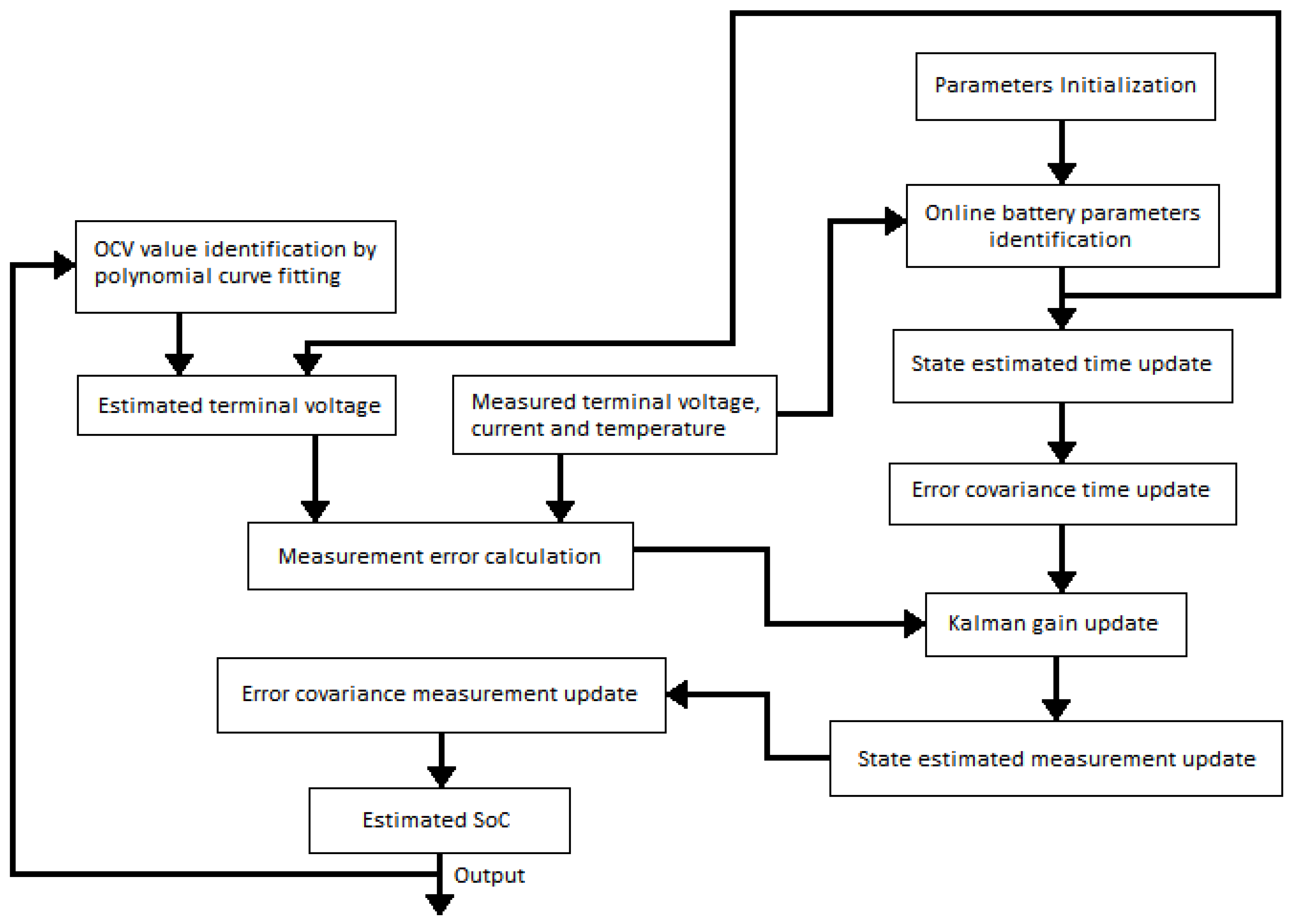
3.1. Using EKF

The Kalman filter (KF) is a suitable method for control system operation. It is a recursive function for solving linear filtering problems of discrete data. Unfortunately, the electrochemical characteristic of LIB makes the OCV-SoC characteristic nonlinear. KF cannot apply to this type of application. Therefore, an extended Kalman filter (EKF) should be adopted to fit the nonlinear characteristics of LIB and estimate the SoC.

3.1.1. The Measurement Process of EKF

The measurement process is always affected by some uncertainties in natural environments. The measurement sensors generate the sensor noise and the EV system causes the processing noise. Both kinds of noise prevent BMS from estimating the SoC accurately. Therefore, under this hidden state situation, EKF is a robust filtering algorithm that corrects estimation errors during noisy signal environments. EKF can predict future system values based on past estimations. It adjusts the Kalman gain’s magnitude according to the changing state error to select whether the measured signal or estimated signal can be utilized for the next state SoC estimation. The EKF algorithm equations can be divided into a few equations, such as State time state update and State measurement state update. Figure 3 shows the operating flow chart of EKF.
Equations (11) to (23) show the system equation of the EKF algorithm and below (11) is the initial state error covariance:
S i g m a X = [ 1 e 2 0 0 2 e 4 ]
Equation (12) is the State estimate time update equation.
X ¯ ^ = A . X ^ + B . U
The matrix A is:
A = [ e x p Δ T Γ 0 0 1 ]
where ΔT = Input data sampling time at time t.
The matrix B is:
B = [ B 1 B 2 ]
where
B 1 = Δ T C 1
B 2 = Δ T C m
And
U = input current
Equation (19) is the Error covariance time update equation.
S i g m a X ^ = A . S i g m a X . A + B . Q . B
where Q is the process noise covariance. Equations (19) and (20) are the Kalman gain update equation.
S i g m a Y = C . S i g m a X ^ . C + D . R . D
where R is the measurement noise covariance.
K g a i n = S i g m a X ^ . C S i g m a Y
Equation (21) is the Measurement Error Calculation.
E g a i n = Y m Y e
where Ym is the measurement voltage error and Ye is the estimated voltage error. Equation (22) is the State estimate measurement update equation.
X ^ = X ¯ ^ + K g a i n . E g a i n
Equation (23) is the Error covariance measurement update equation.
S i g m a X = S i g m a X ^ K g a i n . S i g m a Y . K g a i n
The EKF method has good online calculation ability. First, it compares the estimated and measured values. After that, adjust the Kalman gain to match the error size. If a more significant error is detected, the Kalman gain is adjusted significantly to correct the estimated value; if a minor error is detected, the Kalman gain is modified slightly to correct the estimated value.

3.1.2. The Process Noise and Measurement Noise Covariance Consideration

Paper [30,31] demonstrated the relationship and characteristics of the process noise covariance Q and measurement noise covariance R. Therefore, this paper has tried different values of Q and R for estimating the SoC. A small value of R and Q can make estimation more accurate. Equations (24) and (25) show the process and measurement of noise covariance used in this research for the LIB SoC estimation.
The process noise covariance:
Q = 9 ( e 10 )
The measurement noise covariance:
R = 9 ( e 1 )
The Q and R values are set to  9 ( e 10 )  and  ( 9 e 1 ) ,  respectively. In this paper, another set of Q and R values will be used for comparison.

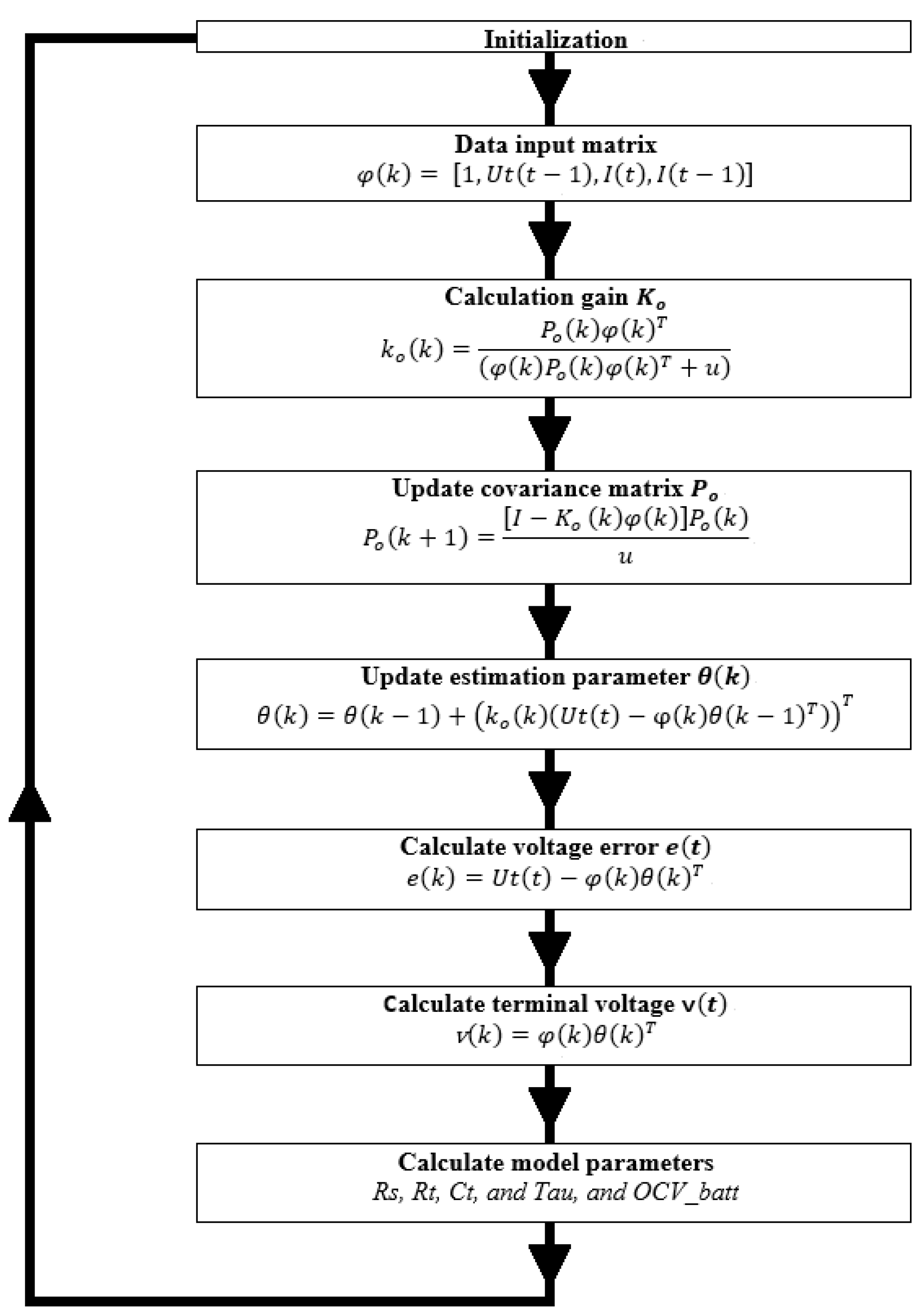
3.2. Using Traditional Mixed Method (Closed-Loop Control System)

The traditional mixed method (MM) is a straightforward self-error correction method for SoC estimation [16]. MM comprises a coulomb counting method (CCM) and a closed-loop control system (CLCS). The CCM method performs the SoC estimation with the rectified voltage error factor generated by the CLCS. It is not difficult to predict the SoC result. However, the drawback of MM is that it can only improve SoC estimation accuracy after certain specific data sampling cycles due to the response time being a bit slow in a noisy environment.

3.3. Using Improved Mixed Method (Dual Closed-Loop Control System)

Due to the drawback of MM, ref. [24], a dual closed-loop control system (DCLCS) is proposed. It can improve the error correction time of the CLCS method and help increase the SoC estimation accuracy. The traditional MM method uses a single CLCS to minimize the voltage error and generate an accurate SoC value. About the DCLCS, one more CLCS is used for the second SoC error correction based on the SoC Root Mean Square Error (RMSE) comparison and evaluated SoC factor. Therefore, DCLCS can improve the response SoC estimation and generate higher accurate SoC estimation results than the traditional MM method.
An Adaptive Error Correction Mechanism (AEC) [24] mechanism is proposed to minimize SoC estimation errors. The AEC supports the DCLCS in adjusting the SoC factor to align with the estimated SoC, ensuring high accuracy in SoC estimation, which is crucial for efficient battery management on the EV platform. Incorporating the AEC can effectively compensate for measurement uncertainties and improve the overall accuracy of SoC estimation in real-world EV applications.

3.4. The Contour of the OCV-SoC Curve at a Low Data Sampling Time Situation

Theoretically, measurement accuracy is proportional to the data sampling time. Figure 4 shows the contour of the OCV-SoC curve at a 1 s data sampling time, and Figure 5 shows the OCV-SoC curve at a 10 s data sampling time. A more accurate and detailed OCV-SoC curve can be obtained if the data sampling time is faster.
A faster data sampling time can acquire more detailed battery information, such as voltage and current data. A 32-bit Microcontroller (MCU) equipped with an external high-speed oscillator can make the system operate faster to collect more voltage and current data for the SoC estimation. Acquisition for fast data sampling time needs, in disguised form, a high-performance hardware cost. Another way to make the BMS system operate faster is to use an MCU’s internal Phase lock loop (PLL) function. However, it is not as accurate as the external high-speed oscillator.

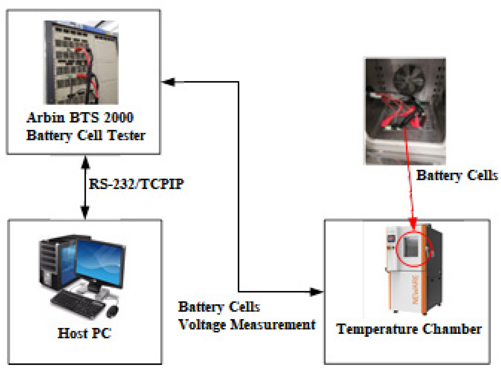
4. Experiments Setup

4.1. Battery Capacity Test at Different Temperatures

Figure 6 shows the laboratory experimental setup for evaluating the SoC estimation. The experiment combines an LFP battery cell, an ARBIN 4-channel battery tester, and a host personal computer (PC). The temperature chamber can maintain the ambient temperature at 25 ± 2 °C during the experiment. The battery cells are placed into the temperature chamber for voltage and current measurement. The battery data is logged and sent to the host PC from the battery tester. The DST voltage and current profile are used as an actual EV application for battery cell testing. Table 1 shows the specifications of the LFP battery cell for the laboratory experiment in detail.

4.2. Dynamic Drive Cycle Test Profile

The Dynamic Stress Test (DST) current profile is used for the battery cell evaluation in the real-time EV application. The battery’s characteristics for these varying loads are measured. The DST can evaluate battery performance in terms of capacity, voltage stability, and temperature change. The DST current and voltage profile are applied in this paper.

4.3. Software Structure for Data Measurement at Different Data Sampling Times

At a real-time measurement, the SoC estimation task in a general BMS software can be implemented by different timer interrupt service routines (ISR). Figure 7 shows the BMS software operation flow chart with specific timer ISR such as 0.5 s, 1 s, 2 s, 5 s, and 10 s. Battery voltage and current measurement can be carried out among these timers ISR. 0.5 s is the fastest ISR, and 10 s is the slowest ISR for data sampling.

4.4. Evaluation Matrices—The Equation of the SoC RMSE

RMSE stands for Root Mean Square Error, which is used for the error evaluation in this paper. It measures the difference between the estimated SoC and the actual measured SoC. Equation (26) shows the calculation of the RMSE. A lower RMSE indicates a more accurate SoC estimation result.
S o C _ R M S E = 1 N k 1 N ( ( E s t i m a t e d ) k ( M e a s u r e d ) k )

5. Results and Discussion

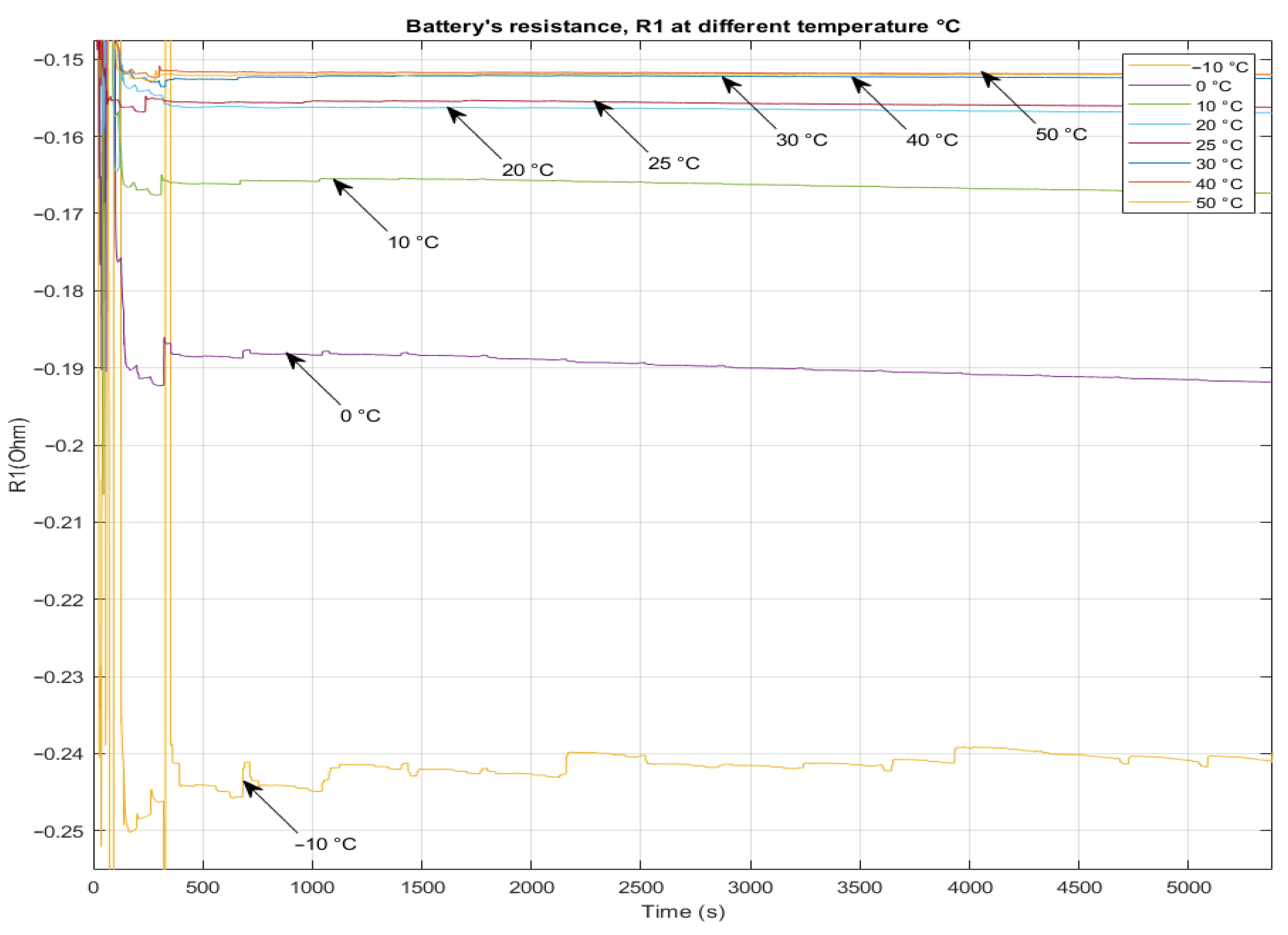
5.1. The Variation of Battery Parameters at Different Temperatures

Figure 8 shows that various  R 0  can be generated at different temperatures during the discharging process of LIB. When the LIB is discharged in an extremely low-temperature environment, for example, at 10 °C, it causes a higher  R 0  (around 0.25 Ohm).
When the LIB is discharged in an extremely high-temperature environment, such as 50 °C, a lower  R 0  (around 0.16 Ohm) can be acquired. It proved that the 1-RC ECM includes the thermal characteristics of LIBs. For the SoC estimation, the 1-RC ECM compensates for the measurement errors caused by the operating temperature variation.
Figure 9 and Figure 10 also show the relationship between battery parameters ( R 1 C 1 ) and operating temperatures. According to these reliable relationships, the model-based EKF can generate an accurate SoC estimation at different temperatures. In the next section, the performance of model-based EKF will be verified step by step.

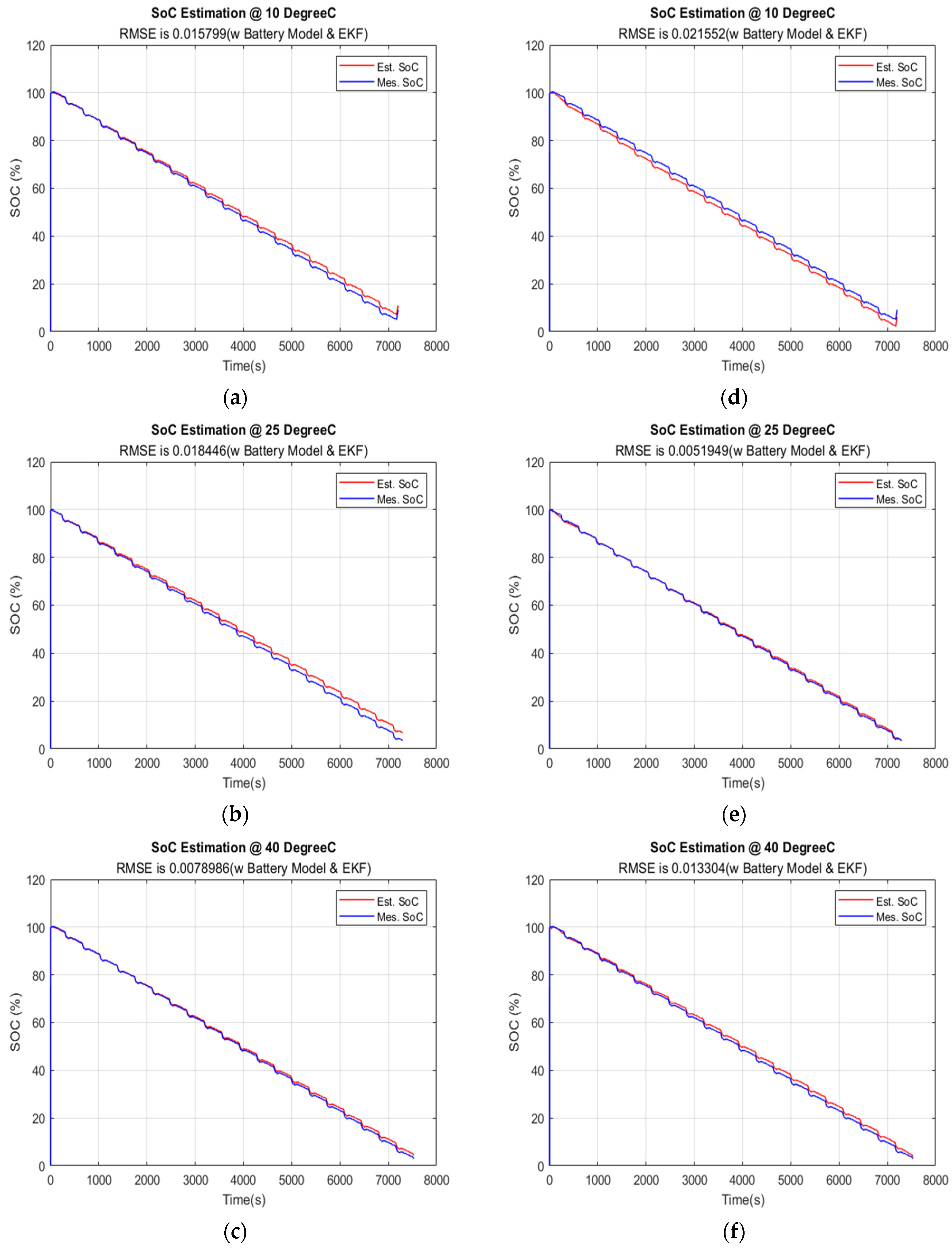
5.2. The SoC Estimation Results at Temperatures 10 °C, 25 °C, and 40 °C by EKF

In this section, a model-based EKF is used to examine the performance of the battery SoC estimation at 25 °C room temperature. The data sampling time is 1 s, and the process noise covariance,  Q = 9 ( e 10 )  and the measurement noise covariance,  R = 9 ( e 1 ) , are applied. Using the DTS for SoC verification, Figure 11 shows that the model-based EKF can accurately estimate the SoC of the battery at the temperatures mentioned above.
Figure 11a,d show that at an operating temperature lower than 25 °C, the battery capacity at discharge mode should be smaller than that at 25 °C. The temperature impacts the battery’s chemistry and lowers the battery’s SoH to less than 100%. Thus, it is a harsh ordeal for the algorithm. Through the DST, the SoC result of EKF can be examined at different temperatures as follows.
Figure 11b,e show the comparison result between the estimated SoC and the actual SoC. There is no difficulty for the EKF in estimating the SoC of the battery with 1-RC ECM. The EKF can converge the estimated and actual SoC to generate an accurate result quickly at 25 °C. The RMSE is 0.018446. To improve the accuracy of the SoC estimation result, another set of noise covariances is applied. The process noise covariance  Q = 9 ( e 150 ) ,  and the measurement noise covariance  R = 9 ( e 49 ) ,  are used for the SoC estimation. Figure 11e shows the RMSE value is 0.0051949, which is better than the values shown in Figure 11b. The experiment shows that changing the Q and R can improve the Kalman filter’s performance and the accuracy of SoC estimation. Table 2 shows the SoC RMSE values at 10 °C, 25 °C, and 40 °C.
The values show that EKF could generate an accurate estimation result with suitable covariance values, Q and R. Table 2 shows that the more accurate SoC result only happened at specific temperatures, 25 °C and 40 °C. The lower temperature situation would decrease the battery capacity and SoH. The EKF cannot rely on accurate battery parameters to estimate the SoC value. Therefore, adjusting the covariance Q and R could be an excellent direction to determine an accurate SoC result for wide-range temperatures.

5.3. The SoC Estimation Result at Temperatures 10 °C, 25 °C, and 40 °C by CLCS and DCLCS with AEC

In this section, model-based methods, CLCS and DCLCS are used to examine the performance of SoC estimation at 25 °C room temperature. The data sampling time is 1 s, and AEC is applied. Using the DST for SoC verification, the RMSE value of the estimated SoC result using DCLCS with AEC is smaller than the estimated SoC result using CLCS.
In this section, using the dynamic load profile of DST, a series of estimated SoC RMSE results are generated and analyzed to prove the superiority of the DCLCS method with AEC over the CLCS. Table 3 compares the SoC-RMSE results of the model-based SoC estimation utilizing CLCS and DCLCS (with AEC) under DST dynamic load profile testing.
Table 3 shows that at 10 °C, the estimated SoC RMSE using CLCS and DCLCS (with AEC) are 0.0209 and 0.0130, respectively. At 25 °C, the estimated SoC RMSE using CLCS and DCLCS (with AED) are 0.0143 and 0.006, respectively. At 40 °C, the estimated SoC RMSE using CLCS and DCLCS (with AED) are 0.0081 and 0.0078, respectively.
It proved that DCLCS (with AEC) generally performs the best at 1 s because it generates a lower SoC RMSE value than the CLCS. Moreover, DCLCS (with AEC) can manage several changeable factors, such as voltage, current, and temperature, which can cause the SoC results to be erroneous. It can generate an accurate online SoC value in actual EV applications without any pre-deterministic step in the laboratory.

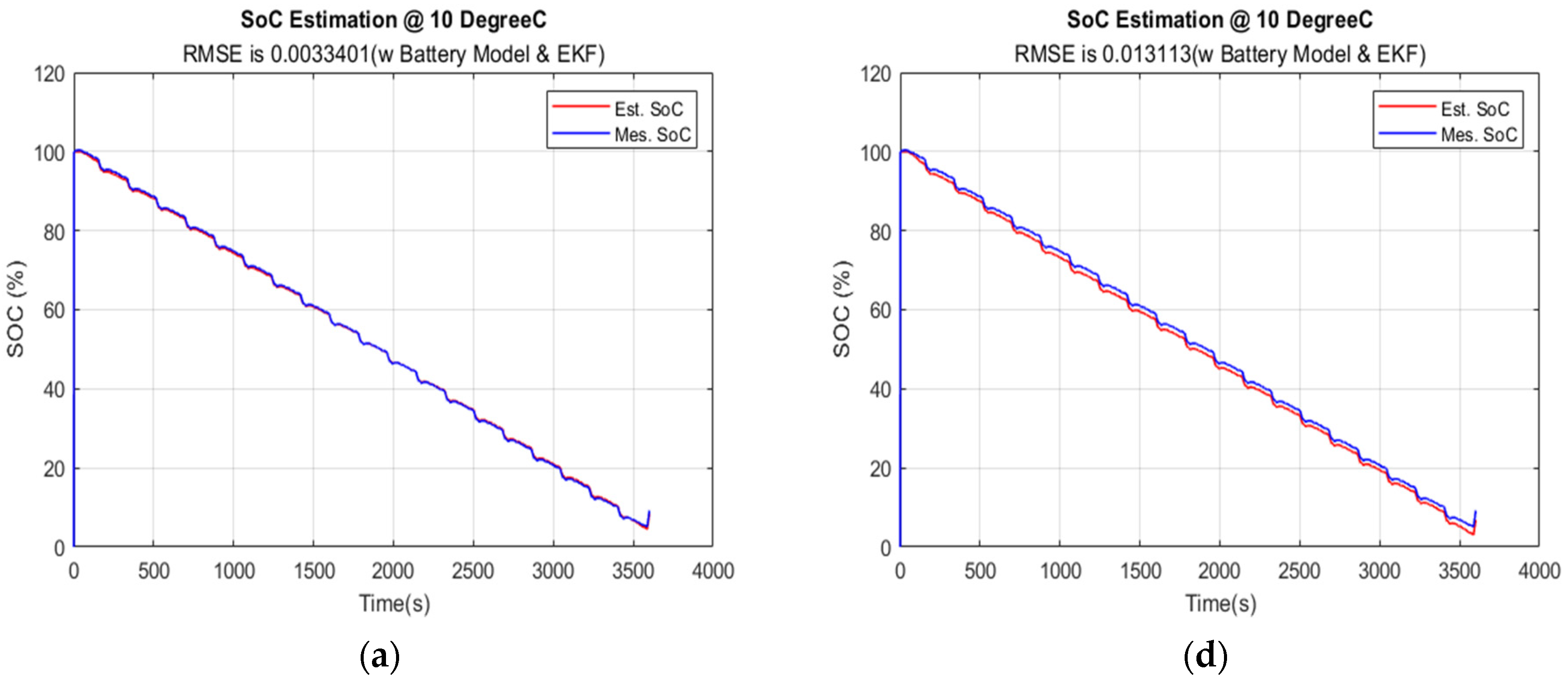
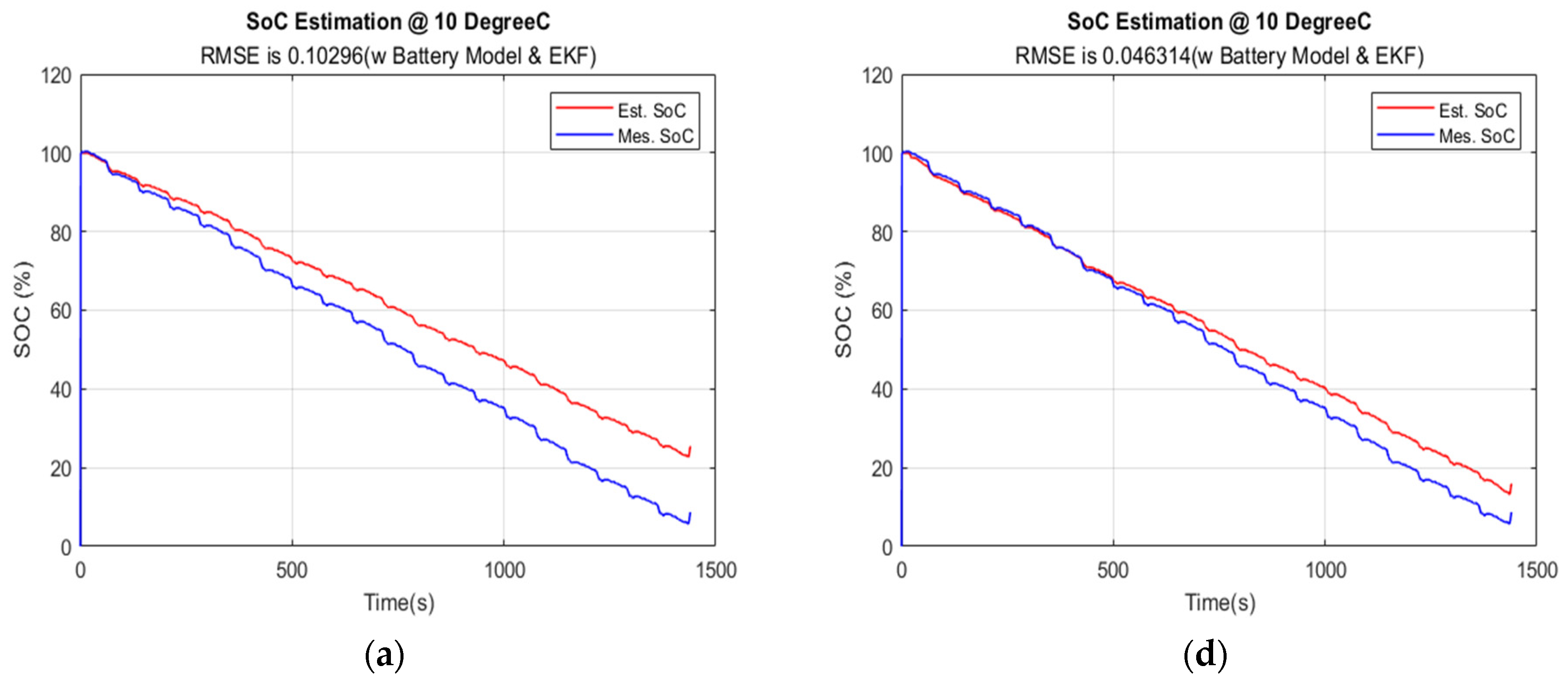
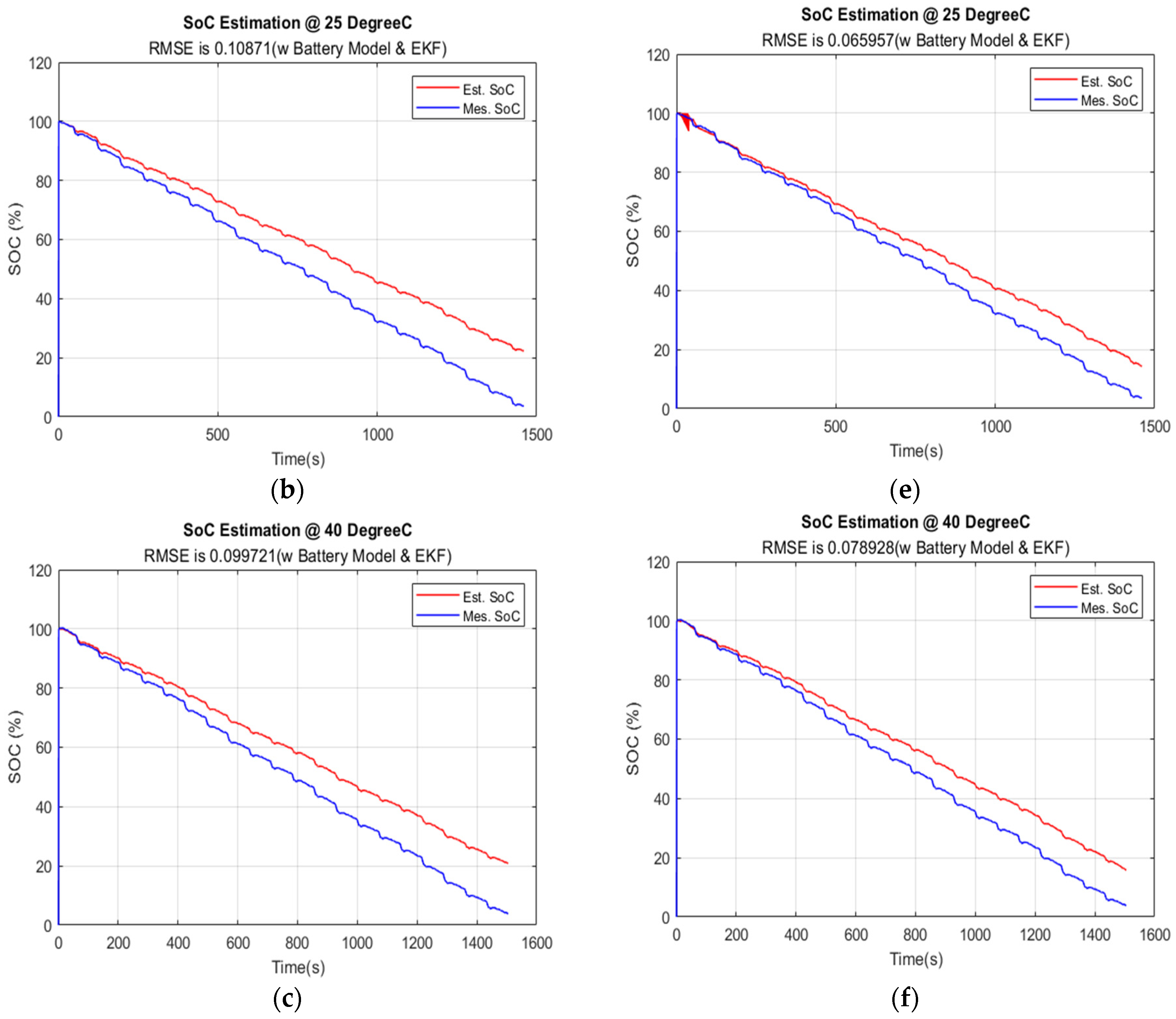
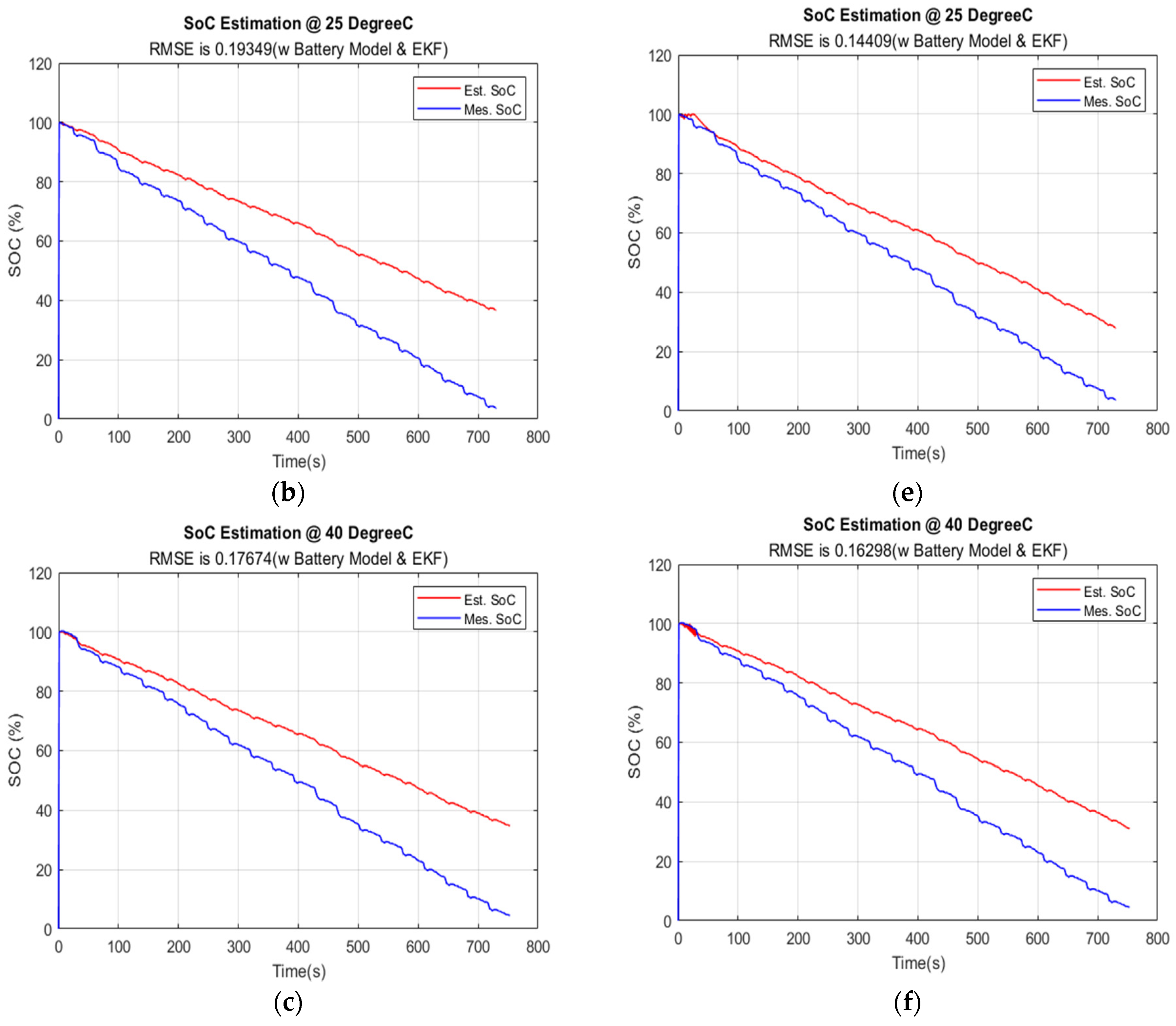
5.4. The SoC Results at Different Data Sampling Times and Temperatures 10 °C, 25 °C, and 40 °C by EKF

Per the experiments in the previous section, EKF can perform well on 1 s data sampling time at different covariances Q and R. However, it is not easy to find the best covariance value. This section will continue to carry out more meaningful experiments to evaluate the performance of EKF at different data sampling times. There is a strong relationship between the EKF algorithm and data sampling time. Faster or slower data sampling time would affect the accuracy of the SoC estimation result. The experiments below show that the variation in sampling time during the estimation process significantly affects the accuracy of the SoC results.

5.4.1. Data Sampling Time at 2 s

For the experiment at 2 s data sampling time, two different sets of covariance, Q and R were still used to generate the SoC estimation result. Figure 12a–f shows that each set of Q and R can generate an accurate SoC estimation result but not at the same temperature.

5.4.2. Data Sampling Time at 5 s

For the 5 s data sampling time experiment, Figure 13a–c show that the EKF still cannot converge the estimated and actual SoC due to the low data sampling time at 10 °C, 25 °C, and 40 °C. However, adjusting the covariances, Q: and R: can improve the overall performance of the EKF on SoC estimation. Figure 13d–f show that a suitable Q and R shall be necessary for improving the accuracy of model-based battery estimation. However, the EKF still does not have enough battery data to correct the error and estimate the SoC accurately. As a result, the SoC is still wrong.

5.4.3. Data Sampling Time at 10 s

Figure 14a–c show that the EKF cannot converge the estimated and actual SoC at 10 °C, 25 °C, and 40 °C due to a prolonged data sampling time. At a 10 s data sampling time, a lot of data is missing. The situation is similar to the result at 5 s data sampling time, even worse. The EKF does not have enough battery data to correct the error and estimate the SoC accurately. As a result, the SoC is wrong.

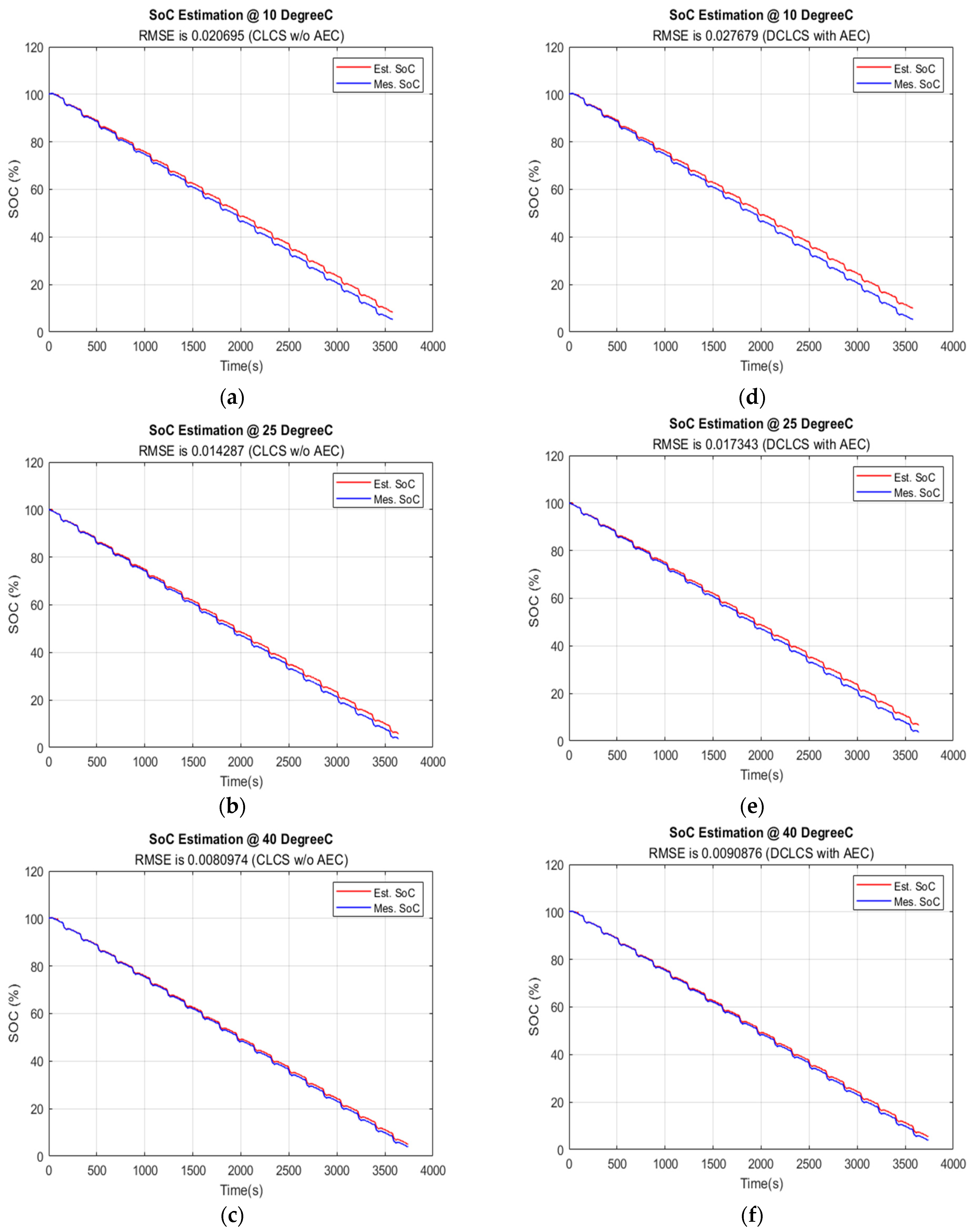
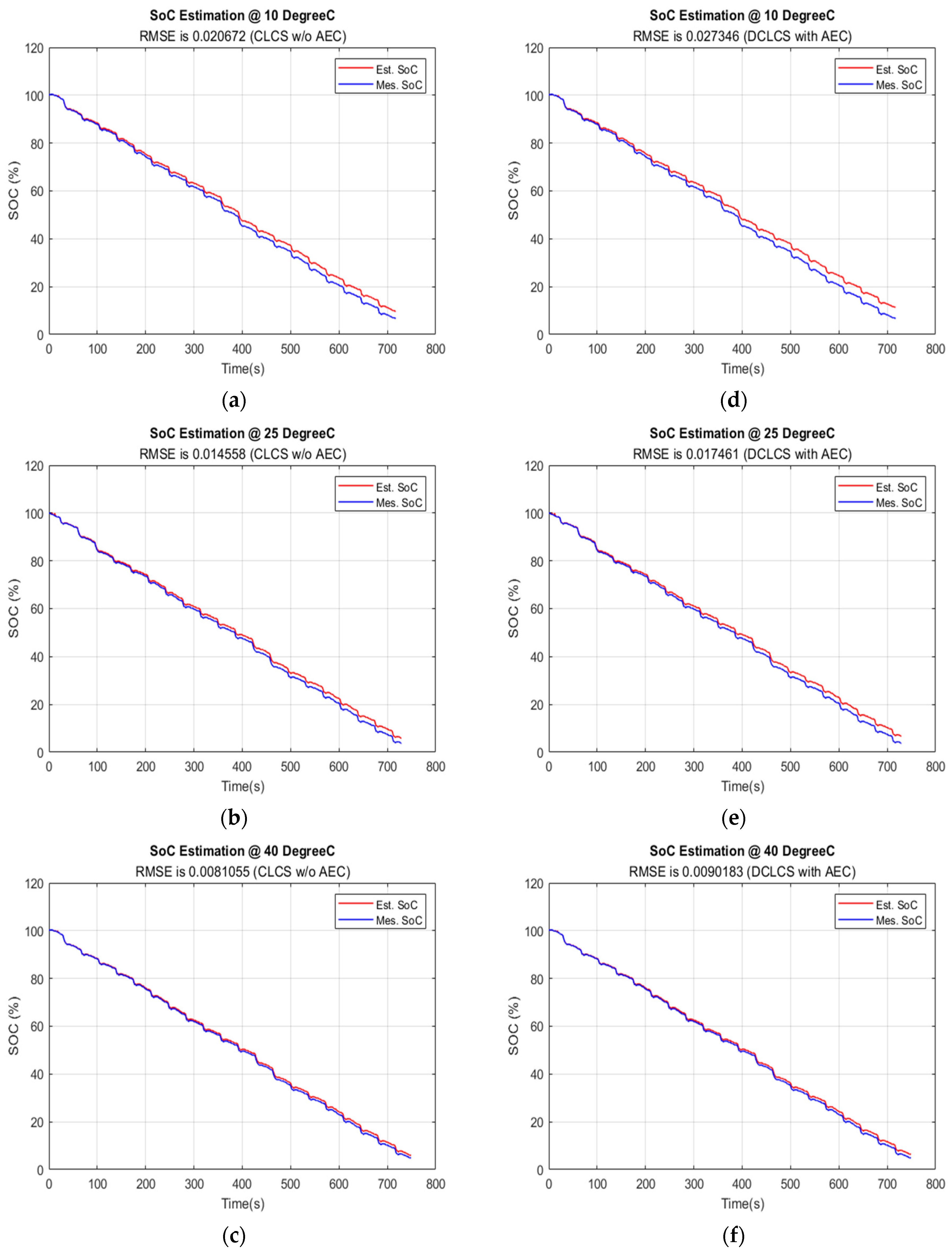
5.5. The SoC Results at Different Data Sampling Times and Temperatures 10 °C, 25 °C, and 40 °C by CLCS and DCLCS

Per the experiment in the previous section, CLCS and DCLCS can perform well at 1 s data sampling time. This section will continue to carry out more meaningful experiments to evaluate the performance of the closed-loop control system at different data sampling times and operating temperatures. CLCS and DCLCS have their characteristics in various environments. Faster or slower data sampling time would affect the SoC estimation accurately. The experiment below shows that the variation in sampling time during the estimation process significantly affects the accuracy of SoC results.

5.5.1. Data Sampling Time at 2 s

When changing the data sampling time from 1 s to 2 s, the accuracy of the SoC estimation result by CLCS is improved. Figure 15 shows that at temperatures of 10 °C, 25 °C, and 40 °C, the RMSE values are 0.020695, 0.014287, and 0.0080974. This result is more accurate than the result by DCLCS at the same temperature environment. The reason is that the response time of CLCS is slower than DCLCS. Therefore, the experiment reflected that operating at a slower data sampling time is beneficial for CLCS when estimating the battery SoC. On the contrary, a lack of battery data would decrease the estimation accuracy of DCLCS.

5.5.2. Data Sampling Time at 5 s and 10 s

Figure 16 and Figure 17 show that at 5 s and 10 s data sampling times, DCLCS’s SoC estimation accuracy is still lower than CLCS’s; the situation is the same as it was at 2 s data sampling time.

5.6. Discussion of Estimation Results of Model-Based Methods

Table 4, Table 5 and Table 6 compare different model-based methods, EKF, MM with CLCS, and DCLCS with AED.
Table 4 and Table 5 show the result of SoC RMSE at a 1 s and 2 s data sampling time, which is smaller and better than that of the 5 s and 10 s. Especially at 10 °C and 25 °C, the EKF can quickly converge the estimated and actual SoC. However, it is based on the covariance values, Q and R. Table 5 shows that the value of the  Q = 9 ( e 150 )  and  R = 9 ( e 49 )  would make the EKF generate a better result at a 1 s data sampling time at 25 °C. Table 4 shows the best SoC estimation result at 2 s of data sampling time compared with other data sampling times at 10 °C. Table 6 shows that the EKF can generate a good result at a 1 s data sampling time at 40 °C. In the 2 s result, there is a correlation between the Q and R parameters, sampling rate, and temperature. The same set of Q and R values cannot be applied to all situations. An adaptive mechanism should be developed to estimate the SoC value by adjusting the Q and R values according to different sampling rates and temperature environments.
The response time of CLCS is slower than that of DCLCS. It is like a low-pass filter and is not sensitive to signal noise, so the CLCS method cannot be very accurate at 1 and 2 s under the 10 °C, 25 °C, and 40 °C environments. However, it can have average performance at all data sampling times and overall temperature environments.
DCLCS is not significantly restricted by battery model parameters accuracy. It is an enhanced algorithm of CLCS that can overcome the effect of signal noise. Therefore, DCLCS can perform very well at 1 and 2 s. However, due to the lack of battery data at slower sampling times, the SoC estimation results at 2 s, 5 s, and 10 s are not as good as CLCS.

6. Conclusions

This paper has comprehensively reviewed the impact of data sampling time and operating temperature on the performance of model-based SoC estimation by CLCS, DCLCS, and EKF. The 1-RC ECM and FF-RLS are potent methods for identifying LIB parameters for online EV applications. FF-RLS can determine the updated battery parameters,  R 0 R 1 , and  C 1 , according to the operating temperature variation during the iterative model-based calculation. The experiment result shows that battery parameters are inversely proportional to the operating temperature. The characteristics of the battery model are suitable for the SoC estimation under different temperature environments. The CLCS, DCLCS, and EKF algorithms periodically update the accurate SoC value by iterative calculation at a specific data sampling time.
Besides the temperature factor, data corruption caused by strong EMI inside EVs should be considered. It severely degrades the ability of SoC estimation. This paper uses different data sampling times to simulate various degrees of data corruption. Therefore, this paper implemented an in-depth analysis of the impact of data sampling time on the performance of the model-based algorithm. Different model-based algorithm would have their characteristics. The CLCS is the most straightforward method for SoC estimation. The computational cost is low, but the accuracy of SoC estimation is not high. It can provide an average performance at different data sampling times over different temperature environments.
The EKF performs well on SoC estimation at a 1 s and 2 s data sampling time. However, a suitable covariance value shall be applied to adjust the EKF for a more accurate SoC estimation. Identifying correct covariance values for SoC estimation under a wide range of data sampling time requirements is very difficult. An adaptive algorithm for adjusting the covariance value for different data sampling times is necessary, but it is not easy to implement.
The DCLCS with the AED method has fast response time characteristics. It can estimate the SoC accurately at 1 s and 2 s data sampling time situations. However, the SoC accuracy decreases due to the lack of battery information at lower data sampling time. Compared with EKF, the implementation complexity and computational cost are lower.

Author Contributions

Conceptualization, P.S. and K.H.W.; Methodology, P.S. and K.H.W.; Software, K.H.W.; Writing—original draft, K.H.W.; Writing—review & editing, S.M. and P.S.; Supervision, M.S., S.M. and A.S. All authors have read and agreed to the published version of the manuscript.

Funding

This research received no any external funding.

Data Availability Statement

The original contributions presented in the study are included in the article, further inquiries can be directed to the corresponding author.

Conflicts of Interest

The authors declare no conflict of interest.

Abbreviations

EVElectric VehicleCANControl Area Network
EVsElectric VehiclesVCUVehicle Control Unit
LIBLithium BatteryCCMCoulomb Counting Method
BMSBattery Management SystemOCVMOpen Circuit Voltage Method
SoCState of ChargeLFPLifePO4
KFKalman FilterMBMModel-Based Method
EMIElectromagnetic interferenceMMMixed Method
EKFExtended Kalman FilterCLCSClosed-loop control system
OCVOpen-Circuit VoltageICC-AECImproved Coulomb Counting Method with an Adaptive Error Correction
1-RCFirst-OrderDCLCSDual closed-loop control system
2-RCSecond-Order   V t Terminal Voltage
ECMEquivalent Circuit Model   R 0 Ohmic Resistance
FF-RLSForgetting Factor-Based Recursive Least Squares Algorithm   R 1 Polarization Resistance
DSTDynamic Stress Test   C 1 Polarization Capacitance
CCCClimate Change CommitteeVocvVoltage Source
HGVsHeavy-Goods VehiclesMCUMicrocontroller
MSDManual Service DisconnectPLLPhase Lock Loop
EMFElectric and Magnetic FieldPCPersonal Computer
ACAlternative CurrentISRInterrupt Service Routine
DCDirect CurrentASTCAutomatic Data Sampling Time Correction
PCFPolynomial Curve Fittingssecond

References

  1. Sun, A. Why China’s Electric Vehicle Market Is at Full Throttle, Schroders. Available online: https://www.schroders.com/en/global/individual/insights/why-chinas-electric-vehicle-market-is-at-full-throttle/ (accessed on 30 October 2023).
  2. Briefing Document: The UK’s Transition to Electric Vehicles. The UK. 2020. Available online: https://www.theccc.org.uk/wp-content/uploads/2020/12/The-UKs-transition-to-electric-vehicles.pdf (accessed on 31 October 2023).
  3. Lin, X.; Stefanopoulou, A.G.; Perez, H.E.; Siegel, J.B.; Li, Y.; Anderson, R.D. Quadruple Adaptive Observer of the Core Temperature in Cylindrical Li-ion Batteries and their Health Monitoring. In Proceedings of the 2012 American Control Conference (ACC), Montréal, QC, Canada, 27–29 June 2012. [Google Scholar] [CrossRef]
  4. Rodríguez-Iturriaga, P.; Anseán, D.; López-Villanueva, J.A.; González, M.; Rodríguez-Bolívar, S. A method for the lifetime sensorless estimation of surface and core temperature in lithium-ion batteries via online updating of electrical parameters. J. Energy Storage 2023, 58, 106260. [Google Scholar] [CrossRef]
  5. Xu, Y.; Hu, M.; Fu, C.; Cao, K.; Su, Z.; Yang, Z. State of charge estimation for lithium-ion batteries based on temperature-dependent second-order RC model. Electronics 2019, 8, 1012. [Google Scholar] [CrossRef]
  6. Madani, S.S.; Schaltz, E.; Kær, S.K. Review of parameter determination for thermal modeling of lithium ion batteries. Batteries 2018, 4, 20. [Google Scholar] [CrossRef]
  7. Sarrafan, K.; Muttaqi, K.; Sutanto, D. Real-time estimation of model parameters and state-of-charge of lithiumion batteries in electric vehicles using recursive least-square with forgetting factor. In Proceedings of the 2018 IEEE International Conference on Power Electronics, Drives and Energy Systems, PEDES 2018, Chennai, India, 18–21 December 2018; Institute of Electrical and Electronics Engineers Inc.: Piscataway, NJ, USA, 2018. [Google Scholar] [CrossRef]
  8. Rzepka, B.; Bischof, S.; Blank, T. Implementing an extended Kalman filter for SoC estimation of a Li-ion battery with hysteresis: A step-by-step guide. Energies 2021, 14, 3733. [Google Scholar] [CrossRef]
  9. Zhu, M.; Qian, K.; Liu, X. A three-time-scale dual extended Kalman filtering for parameter and state estimation of Li-ion battery. Proc. Inst. Mech. Eng. Part D J. Automob. Eng. 2023, 238, 1352–1367. [Google Scholar] [CrossRef]
  10. Wang, D.; Yang, Y.; Gu, T. A hierarchical adaptive extended Kalman filter algorithm for lithium-ion battery state of charge estimation. J. Energy Storage 2023, 62, 106831. [Google Scholar] [CrossRef]
  11. Aiello, O.; Crovetti, P.S.; Fiori, F. Susceptibility to EMI of a Battery Management System IC for electric vehicles. In Proceedings of the 2015 IEEE International Symposium on Electromagnetic Compatibility (EMC), Dresden, Germany, 16–22 August 2015; IEEE: Piscataway, NJ, USA, 2015; pp. 749–754. [Google Scholar] [CrossRef]
  12. Li, M.; Zhang, Y.; Hu, Z.; Zhang, Y.; Zhang, J. A Battery SOC Estimation Method Based on AFFRLS-EKF. Sensors 2021, 21, 5698. [Google Scholar] [CrossRef]
  13. Hannan, M.A.; Lipu, M.S.H.; Hussain, A.; Ker, P.J.; Mahlia, T.M.I.; Mansor, M.; Ayob, A.; Saad, M.H.; Dong, Z.Y. Toward Enhanced State of Charge Estimation of Lithium-ion Batteries Using Optimized Machine Learning Techniques. Sci. Rep. 2020, 10, 4687. [Google Scholar] [CrossRef]
  14. Lee, J.; Won, J. Enhanced Coulomb Counting Method for SoC and SoH Estimation Based on Coulombic Efficiency. IEEE Access 2023, 11, 15449–15459. [Google Scholar] [CrossRef]
  15. Mohammadi, F. Lithium-ion battery State-of-Charge estimation based on an improved Coulomb-Counting algorithm and uncertainty evaluation. J. Energy Storage 2022, 48, 104061. [Google Scholar] [CrossRef]
  16. Codecà, F.; Savaresi, S.M.; Manzoni, V. The Mix Estimation Algorithm for Battery State-of-Charge Estimator: Analysis of the Sensitivity to Model Errors. 2009. Available online: http://asmedigitalcollection.asme.org/DSCC/proceedings-pdf/DSCC2009/48920/97/2770601/97_1.pdf (accessed on 31 October 2023).
  17. Kadem, O.; Kim, J. Real-Time State of Charge-Open Circuit Voltage Curve Construction for Battery State of Charge Estimation. IEEE Trans. Veh. Technol. 2023, 72, 8613–8622. [Google Scholar] [CrossRef]
  18. Zhang, C.; Jiang, J.; Zhang, L.; Liu, S.; Wang, L.; Loh, P.C. A generalized SOC-OCV model for lithium-ion batteries and the SOC estimation for LNMCO battery. Energies 2016, 9, 900. [Google Scholar] [CrossRef]
  19. Wang, Q.; Gao, T.; Li, X. SOC Estimation of Lithium-Ion Battery Based on Equivalent Circuit Model with Variable Parameters. Energies 2022, 15, 5829. [Google Scholar] [CrossRef]
  20. Aktas, A. Design and implementation of adaptive battery charging method considering the battery temperature. IET Circuits Devices Syst. 2020, 14, 72–79. [Google Scholar] [CrossRef]
  21. Hossain, M.; Saha, S.; Arif, M.T.; Oo, A.M.T.; Mendis, N.; Haque, M.E. A Parameter Extraction Method for the Li-Ion Batteries with Wide-Range Temperature Compensation. IEEE Trans. Ind. Appl. 2020, 56, 5625–5636. [Google Scholar] [CrossRef]
  22. Nissing, D.; Mahanta, A.; Van Sterkenburg, S. Thermal Model Parameter Identification of a Lithium Battery. J. Control Sci. Eng. 2017, 2017, 9543781. [Google Scholar] [CrossRef]
  23. Shrivastava, P.; Soon, T.K.; Idris, M.Y.I.B.; Mekhilef, S.; Adnan, S.B.R.S. Model-based state of X estimation of lithium-ion battery for electric vehicle applications. Int. J. Energy Res. 2022, 46, 10704–10723. [Google Scholar] [CrossRef]
  24. Wu, K.H.; Seyedmahmoudian, M.; Mekhilef, S.; Shrivastava, P.; Stojcevski, A. Lithium-ion battery state of charge estimation using improved coulomb counting method with adaptive error correction. Proc. Inst. Mech. Eng. Part D J. Automob. Eng. 2023, 09544070231210562. [Google Scholar] [CrossRef]
  25. Rajanna, B.V.; Kumar, M.K. Comparison of one and two time constant models for lithium ion battery. Int. J. Electr. Comput. Eng. 2020, 10, 670–680. [Google Scholar] [CrossRef]
  26. Yang, S.; Deng, C.; Zhang, Y.; He, Y. State of charge estimation for lithium-ion battery with a temperature-compensated model. Energies 2017, 10, 1560. [Google Scholar] [CrossRef]
  27. Yu, D.X.; Gao, Y.X. SOC estimation of Lithium-ion battery based on Kalman filter algorithm. Appl. Mech. Mater. 2013, 347–350, 1852–1855. [Google Scholar]
  28. Shrivastava, P.; Soon, T.K.; Idris, M.Y.I.B.; Mekhilef, S.; Adnan, S.B.R.S. Combined State of Charge and State of Energy Estimation of Lithium-Ion Battery Using Dual Forgetting Factor-Based Adaptive Extended Kalman Filter for Electric Vehicle Applications. IEEE Trans. Veh. Technol. 2021, 70, 1200–1215. [Google Scholar] [CrossRef]
  29. Shrivastava, P.; Soon, T.K.; Idris, M.Y.B.; Mekhilef, S. Lithium-ion Battery Model Parameter Identification Using Modified Adaptive Forgetting Factor-Based Recursive Least Square Algorithm. In Proceedings of the Energy Conversion Congress and Exposition—Asia, ECCE Asia 2021, Singapore, 24–27 May 2021; Institute of Electrical and Electronics Engineers Inc.: Piscataway, NJ, USA, 2021; pp. 2169–2174. [Google Scholar] [CrossRef]
  30. Zheng, X.; Zhang, Z. State of charge estimation at different temperatures based on dynamic thermal model for lithium-ion batteries. J. Energy Storage 2022, 48, 104011. [Google Scholar] [CrossRef]
  31. Singh, Y.; Mehra, R.; Scholar, M.E. Relative Study of Measurement Noise Covariance R and Process Noise Covariance Q of the Kalman Filter in Estimation. IOSR J. Electr. Electron. Eng. 2015, 10, 112–116. Available online: https://www.iosrjournals.org/iosr-jeee/Papers/Vol10-issue6/Version-1/P01061112116.pdf (accessed on 31 October 2023).
Figure 1. The 1−RC battery model for Li-ion battery SoC estimation.
Energies 17 04791 g001
Figure 2. The flow chart of battery modeling using the FF-RSL algorithm.
Energies 17 04791 g002
Figure 3. The operating software flow chart of SoC estimation by using EKF.
Energies 17 04791 g003
Figure 4. OCV with 1 s data sampling time.
Energies 17 04791 g004
Figure 5. OCV with 10 s data sampling time.
Energies 17 04791 g005
Figure 6. Experiment setting.
Energies 17 04791 g006
Figure 7. Flow chart of BMS software for data measurement by using different interrupt service routines.
Energies 17 04791 g007
Figure 8. The characteristic of  R 0  at different ambient temperatures.
Energies 17 04791 g008
Figure 9. The characteristic of  R 1  at different operating temperatures.
Energies 17 04791 g009
Figure 10. The characteristic of  C 1  at different operating temperatures.
Energies 17 04791 g010
Figure 11. EKF at 1 s data sampling time;  Q = 9 ( e 10 ) R = 9 ( e 1 ) ; (a) at 10 °C; (b) at 25 °C; (c) at 40 °C. EKF at 1 s data sampling time;  Q = 9 ( e 150 ) R = 9 ( e 49 ) ; (d) at 10 °C; (e) at 25 °C; (f) at 40 °C.
Energies 17 04791 g011
Figure 12. EKF at 2 s data sampling time;  Q = 9 ( e 10 ) R = 9 ( e 1 ) ; (a) at 10 °C; (b) at 25 °C; (c) at 40 °C. EKF at 2 s data sampling time;  Q = 9 ( e 150 ) R = 9 ( e 49 ) ; (d) at 10 °C; (e) at 25 °C; (f) at 40 °C.
Energies 17 04791 g012aEnergies 17 04791 g012b
Figure 13. EKF at 5 s data sampling time;  Q = 9 ( e 10 ) R = 9 ( e 1 ) ; (a) at 10 °C; (b) at 25 °C; (c) at 40 °C. EKF at 5 s data sampling time;  Q = 9 ( e 150 ) R = 9 ( e 49 ) ; (d) at 10 °C; (e) at 25 °C; (f) at 40 °C.
Energies 17 04791 g013aEnergies 17 04791 g013b
Figure 14. EKF at 10 s data sampling time;  Q = 9 ( e 10 ) R = 9 ( e 1 ) ; (a) at 10 °C; (b) at 25 °C; (c) at 40 °C. EKF at 10 s data sampling time;  Q = 9 ( e 150 ) R = 9 ( e 49 ) ; (d) at 10 °C; (e) at 25 °C; (f) at 40 °C.
Energies 17 04791 g014aEnergies 17 04791 g014b
Figure 15. CLCS method at 2 s data sampling time; (a) at 10 °C; (b) at 25 °C; (c) at 40 °C. DCLCS with AED method at 2 s data sampling time; (d) at 10 °C; (e) at 25 °C; (f) at 40 °C.
Energies 17 04791 g015
Figure 16. CLCS method at 5 s data sampling time; (a) at 10 °C; (b) at 25 °C; (c) at 40 °C. DCLCS with AED method at 5 s data sampling time; (d) at 10 °C; (e) at 25 °C; (f) at 40 °C.
Energies 17 04791 g016
Figure 17. CLCS method at 10 s data sampling time; (a) at 10 °C; (b) at 25 °C; (c) at 40 °C. DCLCS with AED method at 10 s data sampling time; (d) at 10 °C; (e) at 25 °C; (f) at 40 °C.
Energies 17 04791 g017
Table 1. The specification of the LFP battery cell.
Battery ModelA123 Lithium-Ion Battery
ChemistryLiFePO4 (LFP)
Nominal Capacity1100 mAh
Voltage Range2.0 V to 3.6 V
Nominal Voltage3.3 V
Cell Length65 mm
Diameter18 mm
Temperature Range−10 °C to 50 °C
Table 2. The SoC RMSE values comparison at temperatures 10 °C, 25 °C, and 40 °C.
Covariances Temperature
QR10 °C25 °C40 °C
  9 ( e 10 )   9 ( e 1 ) 0.0157990.01844600.0078986
  9 ( e 150 )   9 ( e 49 ) 0.0215520.00519490.0133040
Table 3. Results comparison of SoC estimation between CLCS and DCLCS with AEC.
Different Temperatures ConditionClosed Loop Control SystemDual Closed Loop Control System with AEC
10.0 °C0.02090.0130
25.0 °C0.014320.0060
40.0 °C0.008120.0078
Table 4. The comparison of SoC between different temperatures and different data sampling times at 10 °C.
Model-Based Methods
Data Sampling TimesEKF
[Q]  = 9 ( e 10 )  
[R]  = 9 ( e 1 )  
EKF
[Q] = 9 ( e 150 )  
[R]  = 9 ( e 49 )  
MM with CLCSDCLCS with AEC
1 s 0.01579900.02155200.02088400.0130400
2 s 0.00334010.01311300.02069500.0276790
5 s 0.10296000.04631400.02077700.0275460
10 s 0.17161000.12607000.02067200.0273460
Table 5. The comparison of SoC between different temperatures and different data sampling times at 25 °C.
Model-Based Methods
Data Sampling TimesEKF
[Q]  = 9 ( e 10 )  
[R]  = 9 ( e 1 )  
EKF
[Q]  = 9 ( e 150 )  
[R]  = 9 ( e 49 )  
MM with CLCSDCLCS
with AEC
1 s 0.01844600.00519490.01431900.0060284
2 s 0.01830200.00714600.01428700.0173430
5 s 0.10871000.06595700.01437500.0174000
10 s 0.19349000.14409000.01455800.0174610
Table 6. The comparison of SoC between different temperatures and different data sampling times at 40 °C.
Model-Based Methods
Data Sampling TimesEKF
[Q]  = 9 ( e 10 )  
[R]  = 9 ( e 1 )  
EKF
[Q] = 9 ( e 150 )  
[R = 9 ( e 49 )  
MM with CLCSDCLCS
with AEC
1 s 0.00789860.01330400.00811640.0078327
2 s 0.00809930.01683100.00809740.0090876
5 s 0.09972100.07892800.00818120.0088326
10 s 0.17674000.16298000.00810550.0090183
Disclaimer/Publisher’s Note: The statements, opinions and data contained in all publications are solely those of the individual author(s) and contributor(s) and not of MDPI and/or the editor(s). MDPI and/or the editor(s) disclaim responsibility for any injury to people or property resulting from any ideas, methods, instructions or products referred to in the content.

