Abstract
The primary objective of this study is to evaluate the accuracy of different forecasting models for monthly wind farm electricity production. This study compares the effectiveness of three forecasting models: Autoregressive Integrated Moving Average (ARIMA), Seasonal ARIMA (SARIMA), and Support Vector Regression (SVR). This study utilizes data from two wind farms located in Poland—‘Gizałki’ and ‘Łęki Dukielskie’—to exclude the possibility of biased results due to specific characteristics of a single farm and to allow for a more comprehensive comparison of the effectiveness of both time series analysis methods. Model parameterization was optimized through a grid search based on the Mean Absolute Percentage Error (MAPE). The performance of the best models was evaluated using Mean Bias Error (MBE), MAPE, Mean Absolute Error (MAE), and R2Score. For the Gizałki farm, the ARIMA model outperformed SARIMA and SVR, while for the Łęki Dukielskie farm, SARIMA proved to be the most accurate, highlighting the importance of optimizing seasonal parameters. The SVR method demonstrated the lowest effectiveness for both datasets. The results indicate that the ARIMA and SARIMA models are effective for forecasting wind farm energy production. However, their performance is influenced by the specificity of the data and seasonal patterns. The study provides an in-depth analysis of the results and offers suggestions for future research, such as extending the data to include multidimensional time series. Our findings have practical implications for enhancing the accuracy of wind farm energy forecasts, which can significantly improve operational efficiency and planning.
1. Introduction
In today’s world, faced with global challenges related to climate change and the depletion of natural resources, the increasing importance of renewable energy and energy storage systems is becoming an indispensable element of our future environment and economy [1]. Renewable energy can ensure energy stability and independence from volatile energy commodity markets [2]. The most popular sources of green energy include solar [3,4], wind [5], hydro [6], and geothermal energy [7,8]. Innovative economies are rapidly transitioning away from fossil fuels in favor of renewable energy sources [9], and such dynamic changes also necessitate the development of forecasting as a key element of a successful energy transition.
The development of advanced forecasting methods plays a crucial role in the effective transition to sustainable energy sources [10]. Forecasting enables the precise determination of the potential and efficiency of renewable technologies by predicting energy production and consumption. Forecasting models operate in various ways, analyzing both single time series and complex multidimensional dependencies, such as atmospheric and seasonal conditions, to predict the future. In the context of the growing importance of renewable energy, further progress in forecasting methods is essential for achieving energy stability.
One branch of forecasting is autoregressive models, which are based on the assumption that future values of the dependent variable can be predicted based on its past values. These models are widely used in time series analysis, allowing for forecasting based on historical data related to the production and consumption of renewable energy. Autoregressive models take into account both short-term and long-term trends and seasonal changes in energy production, which is crucial for the precise management of energy systems based on renewable sources [11].
Autoregressive models are diverse and include a range of techniques used for forecasting. One popular approach is the ARIMA model (Autoregressive Integrated Moving Average), which integrates autoregression (AR) and moving average (MA). ARIMA is effective in modeling time series characterized by non-stationarity, allowing for forecasting based on past observations and seasonal trends [12]. Another advanced version is SARIMA (Seasonal ARIMA), which extends the ARIMA model by also considering seasonal differences in the data, which is crucial for the variability in renewable energy production related to weather conditions and seasonal changes in energy consumption. Additionally, autoregressive models can be extended to various degrees of complexity, including modeling multidimensional dependencies and integrating with other forecasting methods [13], allowing for more accurate predictions in various scenarios of renewable energy applications.
These models are effectively used for forecasting in various fields. For example, reference [14] discussed the methodology of time series analysis and the application of ARIMA and SARIMA models for forecasting currency exchange rates in detail. In [15], ARIMA, SARIMA, and Long Short-Term Memory (LSTM) methods were compared for their effectiveness in sales forecasting. The authors noted that the LSTM method achieved the best results, obtaining a slight advantage in forecast accuracy at the cost of extended execution time over statistical models.
In [16], the study evaluates short-term offshore wind speed forecasting using a SARIMA model, compared to deep learning models Gated Recurrent Unit (GRU) and LSTM. The authors apply SARIMA to hourly wind speed data collected from a coastal met mast in Scotland. Despite the advancements in machine learning, the SARIMA model outperformed GRU and LSTM in forecasting accuracy. The study highlights SARIMA’s effectiveness in capturing seasonal patterns and providing reliable predictions, even with the complexity of offshore wind conditions. The paper underscores the advantages of SARIMA over more complex neural network models, which may suffer from overfitting.
On the other hand [17] presents a hybrid approach using parallel genetic algorithms (GA) to optimize the Seasonal ARIMA (SARIMA) model for forecasting weather data. Traditional ARIMA and SARIMA models are widely used for time series forecasting, but they often struggle with local optima problems. The proposed parallel GA-SARIMA method integrates a genetic algorithm to optimize model parameters, addressing this limitation. Tested on the NCDC dataset for forecasting the mean temperature in India from 2000 to 2017, the parallel GA-SARIMA model significantly improves forecasting accuracy and reduces computational time compared to standard SARIMA models.
In contrast, reference [18] introduces a novel approach by integrating Functional Data Analysis (FDA) with traditional time series models to enhance wind speed forecasting. While conventional models like ARIMA and SARIMA are commonly used, they often fall short in capturing the complex, site-specific, and intermittent nature of wind speed data. The study leverages FDA to model daily wind speed profiles as continuous functions, which allows for a more comprehensive representation of wind patterns. Evaluated against various benchmarks, including ARIMA and neural networks, the FDA-based models, particularly FARX(p), demonstrate superior performance with reduced forecasting errors and effective handling of seasonal and site-specific variations. This approach highlights the potential of FDA in addressing the limitations of traditional models and improving forecast accuracy in wind energy applications.
Conversely, reference [19] proposes an advanced methodology by integrating LSTM networks with seasonal decomposition techniques to enhance wind energy production forecasting. Traditional models such as ARIMA and SARIMA often struggle with the intricate, non-stationary, and seasonal characteristics of wind energy data. By incorporating LSTM networks, which are adept at capturing long-term dependencies and nonlinearities, this study improves the prediction accuracy for wind energy production. When benchmarked against conventional models and other machine learning approaches, the LSTM-enhanced models, especially when combined with STL decomposition, show notable improvements in forecasting precision and robustness in handling seasonal and site-specific dynamics. This approach underscores the efficacy of merging advanced neural networks with decomposition methods to address the shortcomings of traditional forecasting techniques and achieve more reliable wind energy predictions.
Machine learning models, which are often used for time series prediction, are typically treated as a separate group distinct from autoregressive models [20]. They include various techniques capable of capturing complex, nonlinear dependencies in the data. Unlike traditional autoregressive models, machine learning models do not require assumptions about linearity and can process large amounts of data, learning directly from them. As a result, they can be successfully applied in time series forecasting [21]. For instance, in [22], a convolutional neural network (CNN) was used to predict raw milk prices based on contextual representations obtained from time series data. In [23], a discrete wavelet transform combined with artificial neural networks (ANN) was used to forecast river water temperature based on daily measurements of water and air temperature. In [24], a proposal was made to extend the LSTM method by creating a network composed of multiple LSTM layers whose parameterization is determined using a genetic algorithm. The new DLSTM method was used to predict oil production.
In this study, we operate on univariate time series [25]. It should be noted that generally, more data allows for better results, therefore future research aimed at improving the results obtained so far should include extending the studied data to multidimensional time series [26,27].
This work analyzes the effectiveness of models in forecasting wind energy production using two independent wind farms in Poland as examples. Grid search for parameter optimization was also tested as an alternative method for fitting models to data. Finally, the results were compared, considering not only different methods, but also the results obtained from both wind farms to identify the time series data structure’s impact on the results.
2. Materials and Methods
2.1. Data Used
The data for forecasting were obtained from two wind farms located in Poland. The first, Gizałki Wind Farm, was launched in the summer of 2015 and consists of eighteen wind turbines, each capable of producing up to 2 MW of electricity per hour. The second farm, Łęki Dukielskie Wind Farm, has been operational since May 2011 and includes five turbines, each with a capacity of approximately 2 MW, totaling 10 MW. The two wind farms are almost 400 km apart, characterized by different wind conditions, making them interesting research subjects for forecasting electricity production. For the Gizałki farm, data from all turbines was used, but for the Łęki Dukielskie farm, due to the unavailability of data, measurement data from only one turbine was utilized.
The original data were sampled every 10 min. They were aggregated into monthly periods and summed for all turbines in both farms. A few data points were missing, and these missing values were filled with the average values for each turbine, calculated over the entire operational period of the turbine. It should be noted that the number of missing values was minimal, and their impact on the overall data should be negligible.
The data range used for the Gizałki wind farm spanned from August 2015 to March 2022, resulting in 80 values. The energy production from the Gizałki farm is shown in Figure 1.

Figure 1.
Electricity production (GWh) by the Gizałki wind farm over consecutive months.
The data range for the Łęki Dukielskie farm was slightly longer, extending from May 2013 to February 2022, resulting in 106 monthly values. The production graph for the Łęki Dukielskie farm is shown in Figure 2.
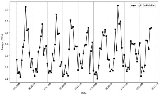
Figure 2.
Electricity production (GWh) by the Łęki Dukielskie wind farm over consecutive months.
Based on the graph, it can be observed that the energy production for both farms has an oscillatory character for annual periods. For the Gizałki farm, the highest production occurs from December to March, while the lowest energy production occurs from June to September. In contrast, for the Łęki Dukielskie farm, the highest production occurs from November to February, while the lowest energy production occurs from May to August. The differences in energy production between the farms indicate a significant impact of local climatic and meteorological conditions, likely due to the distance between them. The varying data lengths, different numbers of turbines at each farm, and different locations allow for a comprehensive examination of both models and better identification of their effectiveness.
In addition to the basic analysis, we applied the STL (Seasonal-Trend decomposition using locally estimated scatterplot smoothing (LOESS)) method to further investigate the characteristics of energy production data from the wind farms. STL is a powerful technique that decomposes time series data into three components: trend, seasonality, and residuals. The STL graph for the Gizałki farm is shown in Figure 3 and that for the Łęki Dukielskie in Figure 4.

Figure 3.
STL decomposition of monthly electricity production by the Gizałki wind farm. Plots from top to bottom: actual data, trend, seasonality, and residuals (dots).
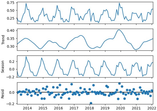
Figure 4.
STL decomposition of monthly electricity production by the Łęki Dukielskie wind farm. Plots from top to bottom: actual data, trend, seasonality, and residuals (dots).
The STL algorithm first estimates the seasonal component by applying LOESS to the data, capturing any recurring patterns within specified seasonal windows. This allows the seasonality to vary over time if needed. After the seasonal component is removed, the trend component is isolated and similarly estimated using LOESS, revealing long-term patterns in the data. The residual component is then calculated by subtracting both the seasonal and trend components from the original time series, representing any remaining variation. STL is particularly robust to outliers and offers flexible decomposition, making it an effective tool for uncovering complex patterns in time series data.
In the STL decomposition for both wind farms, the trend component displays a generally flat pattern with minor variations, without a distinct upward or downward trend over time. This observation suggests that there is no significant long-term trend in energy production over the observed period.
The lack of a clear trend is consistent with the nature of wind energy, where production levels can be influenced by various short-term factors such as changes in wind patterns, rather than showing a consistent annual increase or decrease. Wind speeds and, consequently, energy output tend to be relatively stable year over year, with variability primarily driven by seasonal fluctuations rather than long-term trends.
In the STL decomposition for both wind farms, the seasonal component exhibits oscillations with peaks and troughs occurring at 12-month intervals, reflecting a recurring annual pattern. However, an interesting trend emerges: the first peak of the seasonality component is slightly larger, and subsequent peaks gradually decrease over time. This indicates that, while seasonal fluctuations are still present, the intensity of these fluctuations is decreasing across the observed period what might reflect more stable or less extreme weather conditions in later years. Nonetheless, the persistence of the 12-month oscillations confirms that seasonality remains an important factor influencing the variability in wind energy production, even as its magnitude diminishes.
Additionally, in both cases, amplitudes of increases are slightly larger than those of decreases. This pattern suggests that while the overall fluctuations remain, there is a tendency for positive deviations from the mean to be more pronounced than negative deviations. This could be due to inherent characteristics of wind energy production, where factors such as increased wind speeds or operational changes may cause more significant positive spikes than negative dips. Theoretically, there is no upper limit to the potential increase in energy production, as higher wind speeds can lead to larger energy outputs. However, the minimum value of energy production is constrained by zero, meaning that production cannot fall below this threshold. This asymmetry could contribute to the observed larger amplitudes of positive deviations compared to negative ones.
In the STL decomposition for both wind farms, the residual component shows a pattern where most data points are clustered relatively close to the zero line, with only a few deviations from this baseline. The residuals are plotted against time, and while the majority of points remain near the zero line, indicating that the model has effectively captured the trend and seasonality, there are occasional outliers that deviate more significantly from this central value. These outliers represent periods of unexpected variation in energy production that are not explained by the trend or seasonal components. The presence of such deviations suggests that while the overall model fits the data well, there are still some instances of irregular or extreme fluctuations in energy production that warrant further investigation. This pattern of residuals reflects the inherent variability in wind energy production, where occasional anomalies or unusual events can still occur even in the context of a longer-term trend and seasonal patterns.
Another element that we used to better present the data is represented by the error bars depicted in Figure 5. This graphical representation provides crucial insights into the variability and reliability of energy production estimates for the Gizałki wind farm. By incorporating standard deviations into the visualization, the error bars highlight the range within which the true mean energy production is likely to fall, offering a clearer understanding of the inherent uncertainties and fluctuations in the data. This approach is particularly valuable for assessing the consistency of energy outputs across multiple turbines, as it reflects the combined variability from all 18 turbines at the Gizałki farm. The inclusion of error bars not only enhances the interpretability of the data by illustrating the spread of energy production values, but also helps in identifying periods with significant deviations from the mean, which may indicate anomalies or shifts in operational efficiency. This type of analysis was not feasible for the Łęki Dukielskie wind farm because the data were sourced from only a single turbine.
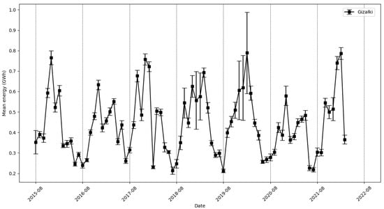
Figure 5.
Mean energy production with standard deviations for the Gizałki wind farm, displayed as error bars.
2.2. Methods Used
Three methods were employed in this study: ARIMA; SARIMA, to investigate how adding a seasonal component affects the accuracy of forecasting data characterized by seasonal oscillations; and SVR to examine whether advanced machine learning techniques can improve forecast accuracy compared to traditional statistical methods. The forecasted data exhibit oscillatory patterns on an annual basis. The ARIMA method models time series by considering past values of the dependent variable and noise, enabling forecasts of future values based on past observations. Meanwhile, the SARIMA method extends the ARIMA model by incorporating a seasonal component, allowing for the inclusion of cyclic patterns in the data. SVR is known for its ability to model complex, nonlinear dependencies in data, which can be advantageous for data with distinct seasonal patterns and irregularities [28].
All methods were tested similarly across extensive parameter grids to select the model best suited to the tested data, as illustrated in Figure 6.

Figure 6.
Schematic of method testing using parameter grid search.
2.2.1. ARIMA
ARIMA is a statistical analysis model particularly useful in time series analysis, both for better understanding data and forecasting future trends [29]. The ARIMA model consists of three main components:
Autoregression (AR)—this means that the value of the variable depends on its previous values. This component describes the parameter p, which determines the number of delays in the autoregressive part. The formula describing this part is (1).
where: α1, α2, …, αp, are autoregression coefficients, εt is white noise (random component).
Integration (I)—data are transformed by differencing, which means removing non-stationarity, such as characteristics of data that change over time, such as mean, trends, or seasonality. This helps to better understand existing patterns in the data and improve the effectiveness of forecasting models that assume time series stationarity. Differencing involves replacing values with differences between successive values of the time series.
This part of the model is associated with the parameter d, which determines the number of differencing needed to make the data stationary. The integration process can be described using recursive Equations (2) and (3).
where: εt, is random disturbance.
The process of changing data can be easily visualized. The top chart in Figure 7 shows random data with a growing trend, meaning non-stationary data. The bottom chart shows the same data after applying single differencing (d = 1), which removed the trend and resulted in stationary data.
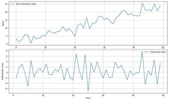
Figure 7.
Visualization of time series integration mechanism.
Moving Average (MA)—the model takes into account dependencies between current values and errors from previous forecasts, which helps to smooth data and improve forecast accuracy. This part of the model is described by the parameter q, which denotes the number of delays in the moving average part. This section is described by Formula (4).
where: Y is the current value at time t, μ is a constant, εt is random disturbance, and θi represents moving average coefficients for delayed disturbance values.
To select the appropriate parameters for the ARIMA model, methods such as the autocorrelation function (ACF) and partial autocorrelation function (PACF) are commonly used [30]. These tools allow for an assessment of how previous time values influence the observation at a given time point. For this study, a method of searching the entire parameter grid was applied, enabling a comprehensive analysis of various combinations of ARIMA parameter values. This is particularly important because it allows for precise fitting of the model to the analyzed time series, taking into account both autocorrelation effects and other factors influencing data dynamics. The difference between the ACF/PACF-based approach and searching the full parameter grid lies in the scope of analysis: the former focuses on direct relationships between observations at different lags, while the latter explores a wide range of parameter combinations to maximize model fit to the data.
2.2.2. SARIMA
The SARIMA model is an extension of the ARIMA model. It is an advanced tool for time series analysis, particularly useful for forecasting data that exhibit both short-term and long-term dependencies and seasonal patterns. It includes all components found in the ARIMA model and adds additional components:
Seasonal Autoregression (SAR)—the seasonal counterpart of the autoregressive component, which considers dependencies between current values and their seasonal predecessors.
Seasonal Integration (SI)—seasonal differencing, which involves subtracting values from previous seasons to remove seasonality.
Seasonal Moving Average (SMA)—the seasonal counterpart of the moving average component, which considers dependencies between current values and errors from previous seasons.
Seasonality—determines the length of the seasonal cycle. Typically, the seasonality value is set equal to the seasonality of the time series on which the prediction is made.
2.2.3. SVR
Support Vector Regression (SVR) is a machine learning algorithm used for regression analysis [31]. The goal of SVR is to find a function that approximates the relationship between input variables and a continuous target variable, minimizing prediction error. SVR is based on the principles of Support Vector Machines (SVM), which are commonly used in classification tasks, but are focused on predicting continuous outcomes.
SVR differs from SVM, which is used for classification, in that it aims to find a hyperplane that best fits the data points in a continuous space. It achieves this by mapping input variables into a higher-dimensional feature space and finding a hyperplane that maximizes the margin (distance) between the hyperplane and the closest data points while minimizing prediction error [32].
The main components of SVR are:
Kernel Function—SVR uses a kernel function to map input data to become more linear and easier to model. Popular kernel functions include radial basis function (RBF), polynomial, and sigmoid.
Epsilon Margin (ε)—SVR introduces the concept of an epsilon margin, where prediction errors are ignored if they fall within a specified range of ε. The goal is to minimize the cost function, which considers both model complexity and prediction errors.
Regularization Parameter (C)—the parameter C controls the trade-off between maximizing the margin and minimizing prediction errors. A high value of C aims to minimize prediction errors at the expense of a narrower margin, whereas a low value of C allows for a wider margin at the expense of larger errors.
2.3. Errors
During the parameter optimization process for both methods, forecast error values were monitored to assess how well each model performed. The errors monitored included MBE (5), MAPE (6), MAE (7), and R2Score (8) [33].
where xi represents the actual value, represents the predicted value, represents the mean value computed from all actual values.
MBE is calculated as the average of the differences between forecasted values and actual values. It helps identify systematic errors in the forecasts by showing whether predictions consistently overestimate or underestimate actual energy production. A positive value denotes a tendency for forecasts to surpass actual values, implying an overpredictive tendency, whereas a negative MBE implies an underestimating tendency. With these data, forecasting models can be modified to decrease bias and increase accuracy. Knowing if projections are unduly optimistic or pessimistic helps with resource management and risk assessment for operational and financial planning. Furthermore, MBE sheds light on the projections’ long-term stability; a near-zero MBE indicates balanced predictions over long time horizons, while large deviations indicate model flaws.
MAPE is a metric used to assess forecast accuracy by calculating the average percentage difference between predicted and actual values. It is computed as the mean of the absolute percentage errors across all forecasts. One of the key advantages of MAPE is that it expresses errors as percentages, which facilitates comparison across different datasets or models. A MAPE of 0% indicates a perfect forecast with no error; conversely, a high MAPE indicates less accurate forecasts. In the context of monthly wind energy forecasts, MAPE is crucial for evaluating forecast precision relative to actual energy production. It helps operators gauge forecast accuracy, informs resource management, and aids in balancing supply and demand.
MAE is calculated as the average of the absolute differences between forecasted values and actual values. This metric provides a straightforward measure of forecast accuracy in the same units as the data (e.g., GWh). MAE reflects the average magnitude of forecast errors without considering their direction, making it a clear indicator of overall forecast precision. A lower MAE indicates better model performance by minimizing the average deviation between forecasts and actual values.
R2Score, or the coefficient of determination, quantifies the proportion of the variance in the dependent variable that is predictable from the independent variables. In the context of wind energy forecasting, R2Score evaluates how well the model explains the variability in actual energy production based on the input data. A value close to 1 indicates that the model explains a high proportion of the variance, reflecting strong predictive power, while a value close to 0 suggests poor model performance. R2 is useful for comparing different forecasting models; however, it should be interpreted with caution, as a high R2 does not always imply a superior model due to potential overfitting.
3. Results
3.1. ARIMA
While fitting the ARIMA model to the data, the objective was to find values for three parameters: p, d, and q. Since these parameters are also used in the second tested method, SARIMA, it was important to search the same parameter grids for both methods. This approach ensures consistency in results and allows for direct comparison. Therefore, two tests were conducted for the ARIMA method: ‘test 1’ with parameter ranges p, d, q identical to SARIMA, and ‘test 2’ with broader parameter ranges. Table 1 presents the grids of searched parameters and the selected optimal parameters for both tests. Range represents the inclusive span of values that were explored for each parameter, while Step indicates the increment with which the specified range was searched for the given parameter.

Table 1.
Grid of searched parameters and selected values for the ARIMA method.
Comparison of different parameterizations of trained models was conducted based on minimizing MAPE error on validation data (last 12 values of the dataset). In both tests, the selected parameter sets achieved models with the lowest MAPE error for both Gizałki and Łęki Dukielskie farms.
3.2. SARIMA
For the SARIMA method, in addition to parameters p, d, q, the objective was also to find values for three additional seasonal parameters: P, D, Q. The parameter s, which controls seasonality, was set to a constant value of 12, corresponding to the annual cycles of energy production in wind farms, which exhibit clear seasonality. Table 2 presents the grid of searched parameters and the selected optimal parameters for Gizałki and Łęki Dukielskie farms.
Table 2.
Grid of searched parameters and selected values for the SARIMA method.
Similar to the ARIMA network, data were compared based on MAPE error, and both selected parameter sets yielded the lowest error values for both wind farms.
3.3. SVR
While adjusting the SVR model to the data, the goal was to find values for five parameters: regularization (C), tolerance margin (ε), kernel parameter (γ), kernel function (kernel), and independent kernel coefficient (ind_term). A broad grid of parameters was searched to find the most optimal values for both wind farms: Gizałki and Łęki Dukielskie. Table 3 presents the ranges of searched parameters and the selected optimal parameters for both locations. If the ‘Step’ column shows ‘log’, it indicates that the parameter values were not distributed linearly, but rather on a logarithmic scale. The ‘Number of steps’ column indicates how many values on the logarithmic scale were distributed. Specific values can be calculated according to the Formula:
where ‘start’ is the initial value from the ‘Range’; ‘stop’ is the final value from the ‘Range’; and ‘num’ is equal to ‘Number of steps’.
Table 3.
Grid of searched parameters and selected values for the SVR method.
3.4. Monthly Forecasts
The forecast results were monthly predictions made using three tested methods for each of the wind farms. For both ARIMA and SARIMA methods, tests were conducted with the same parameter ranges of p, d, q (test 1). For both farms, all methods were tested, and predictions were made for 12 months ahead. Table 4 presents the comparison of these forecasts along with the actual values for the Gizałki wind farm, while Table 5 compiles the forecasts for the Łęki Dukielskie wind farm.
Table 4.
Comparison of actual energy production values by the Gizałki wind farms with predictions made using ARIMA (test 1, test 2), SARIMA, and SVR methods (GWh).
Table 5.
Comparison of actual energy production values by the Łęki Dukielskie wind farms with predictions made using ARIMA (test 1, test 2), SARIMA, and SVR methods (GWh).
Additional tests with an expanded grid of parameters were also conducted for the ARIMA method to check if increasing the parameter range, and thus increasing computation time, would lead to results similar to the more computationally demanding SARIMA method (test 2).
3.5. Error Values
Error values for each method using parameters that resulted in the lowest MAPE error are presented in Table 6.
Table 6.
Error values for the applied methods ARIMA, SARIMA, SVR for the Gizałki and Łęki Dukielskie wind farms.
4. Discussion
The obtained results allow for an assessment of the effectiveness of the applied methods in forecasting monthly electricity production from wind farms.
Gizałki Wind Farm—the SARIMA and SVR methods performed the worst. All error values were worse compared to the ARIMA method in both tests conducted on this farm. Interestingly, SARIMA performed worse than ARIMA with the same parameter grid, which was likely due to the seasonal parameter s. The best result was achieved using the ARIMA method with the wide parameter grid test. Predictions from test 1 using ARIMA were omitted from the plots for clarity, as all tested values were within the parameter grid of test 2.
The results of the best models for the Gizałki farm are presented in Figure 8.
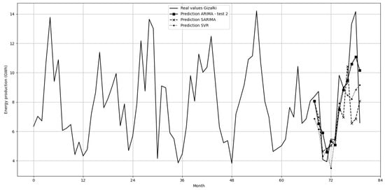
Figure 8.
Prediction of electricity production (GWh) by the Gizałki wind farm in consecutive months using ARIMA, SARIMA, and SVR models.
Łęki Dukielskie Wind Farm—SARIMA achieved the best result among all tests. All error values were better than for both tests of the ARIMA and SVR methods. SARIMA yielded better results than ARIMA with the same parameter grid, indicating the effectiveness of incorporating seasonal parameters in this case.
The results of the best models for the Łęki Dukielskie farm are presented in Figure 9.

Figure 9.
Prediction of electricity production (GWh) by the Łęki Dukielskie wind farm in consecutive months using ARIMA, SARIMA, and SVR models.
Comparing both wind farms, it can be observed that ARIMA, in both tests, yielded smaller percentage errors and higher R² values for the Gizałki farm. In contrast, SARIMA provided significantly better results for the Łęki Dukielskie farm. These discrepancies arise from differences in data from both farms, influencing the model results.
Based on the results presented in the plots, the models performed significantly worse in predicting the energy production of the Gizałki farm, mainly due to the very high local maximum production in January/February 2022, where prediction values deviated the most from the actual values. However, the MAPE and R2Score data did not unequivocally indicate which data were easier to predict. MAPE achieved, on average, smaller values for the Gizałki farm, while R2Score had significantly higher values for the Łęki Dukielskie farm. Additionally, the results indicate that the SVR method performed the worst in both cases. ARIMA achieved the best results for the Gizałki farm, and SARIMA for the Łęki Dukielskie farm, making it difficult to decisively determine the better method.
To further enhance our understanding of the models’ performance, a density plot of the prediction errors was created, providing a clear view of the error distribution for each model. This type of plot is valuable for understanding the distribution and concentration of errors, allowing for a more nuanced comparison between the models. It helps to identify not only the average error, but also the range and frequency of errors, providing deeper insights into model performance.
Figure 10 provides the error density distribution for three models used in forecasting for Gizałki wind farm. All three models share a similar shape, with peaks near zero error, indicating that predictions are centered around actual values. ARIMA shows slightly higher density near zero compared to SARIMA and SVR, suggesting it provides more accurate forecasts for that wind farm. SARIMA, while showing a peak near zero, has the widest distribution and is shifted furthest right, indicating it has more variability in errors. This suggests SARIMA’s performance may vary more significantly depending on the data.
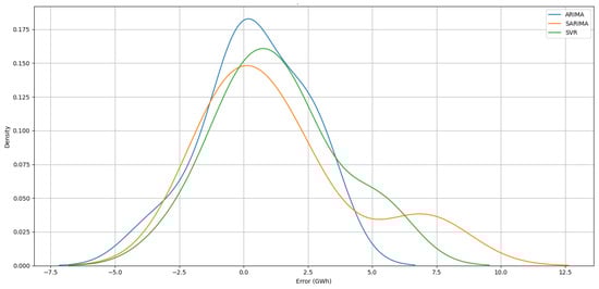
Figure 10.
Density plot of prediction errors for ARIMA, SARIMA, and SVR models for Gizałki wind farm.
Figure 11 illustrates the error density distribution for the three forecasting models. All models exhibit peaks near zero error, indicating that predictions are centered around the actual values. SARIMA achieved the highest peak at zero error, suggesting it performed better for these specific data compared to ARIMA and SVR. SARIMA, ARIMA, and SVR all had similar distributions at the extremes, with no model showing significant deviation.
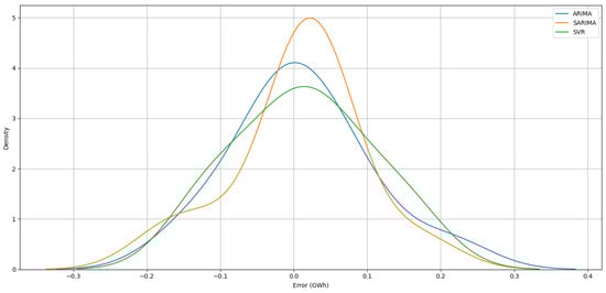
Figure 11.
Density plot of prediction errors for ARIMA, SARIMA, and SVR models for Łęki Dukielskie wind farm.
In summary, the study showed that the ARIMA, SARIMA, and SVR models are capable of accurately forecasting a single-dimensional time series with oscillatory characteristics. The differences in results between the methods were not large, but allowed for the identification of a better method. Despite the presence of seasonality in the data, the SARIMA model may sometimes yield worse results than the ARIMA model. This may indicate the need for a more detailed analysis of data characteristics and optimization of model parameters depending on the specific time series. The measured error values were small, considering the relatively limited amount of data and the fact that the forecasts were based solely on a single time series.
Despite differences in data characteristics, the ARIMA model demonstrated stability, achieving similar results in both tested cases for the Gizałki and Łęki Dukielskie farms. On the other hand, although the SARIMA method yielded better results for the Łęki Dukielskie farm, it achieved significantly worse results for the Gizałki farm. Such variability in the results indicates that the effectiveness of the SARIMA method may depend on the specifics of the data and requires a more detailed analysis and optimization of seasonal parameters. Using the SVR method resulted in similar error values for both data sets, but they were worse than those for the ARIMA/SARIMA methods.
5. Conclusions
The study aimed to compare three methods for forecasting electricity production from wind farms: ARIMA, SARIMA, and SVR. Data for forecasting were obtained from two wind farms located in Poland, the Gizałki and Łęki Dukielskie farms.
Data from both farms exhibited an oscillatory nature over annual periods, although they differed between each other and the oscillations were shifted in time due to the large distance between the farms.
ARIMA performed better for the Gizałki farm, whereas SARIMA performed better for the Łęki Dukielskie farm. SVR performed the worst for both wind farms. Additionally, significant improvements in forecast accuracy were observed for both farms following the expansion of the parameter search grid for the ARIMA method. It was also noted that, even with overlapping parameter grids for p, d, and q, the SARIMA model may have produced inferior results compared to ARIMA due to the defined seasonality.
Based on these findings, both methods can effectively be applied to forecast electricity production from wind farms and generally to oscillatory time series. However, attention should be paid to the specificity of the data and the characteristics of seasonality, which can affect forecast accuracy.
Further research could include a broader range of parameterization, increased dataset sizes in terms of the number of analyzed time series, and exploration of additional methods.
Author Contributions
Conceptualization, K.S. and D.M.; methodology, K.S. and G.D.; software, K.S.; validation, G.D. and J.K.; formal analysis, K.S., D.M. and J.K.; investigation, G.D.; resources, K.S. and J.K.; data curation, D.M.; writing—original draft preparation, K.S. and D.M.; writing—review and editing, K.S. and D.M.; visualization, K.S.; supervision, D.M.; project administration, J.K. All authors have read and agreed to the published version of the manuscript.
Funding
This research was funded by the Bialystok University of Technology as part of the teamwork WZ/WE-IA/3/2023 of the Department of Photonics, Electronics and Lighting Technology, in part by the statutory funds (UPB) of Department of Electrical and Computer Engineering Fundamentals Rzeszow University of Technology.
Data Availability Statement
The data presented in this study are available upon request from the corresponding author.
Conflicts of Interest
The authors declare no conflicts of interest.
References
- Sayed, E.T.; Olabi, A.G.; Alami, A.H.; Radwan, A.; Mdallal, A.; Rezk, A.; Abdelkareem, M.A. Renewable Energy and Energy Storage Systems. Energies 2023, 16, 1415. [Google Scholar] [CrossRef]
- Turco, E.; Bazzana, D.; Rizzati, M.; Ciola, E.; Vergalli, S. Energy price shocks and stabilization policies in the MATRIX model. Energy Policy 2023, 177, 113567. [Google Scholar] [CrossRef]
- Pourasl, H.H.; Vatankhah Barenji, R.; Khojastehnezhad, V.M. Solar energy status in the world: A comprehensive review. Energy Rep. 2023, 10, 3474–3493. [Google Scholar] [CrossRef]
- Hasan, M.M.; Hossain, S.; Mofijur, M.; Kabir, Z.; Badruddin, I.A.; Yunus Khan, T.M.; Jassim, E. Harnessing Solar Power: A Review of Photovoltaic Innovations, Solar Thermal Systems, and the Dawn of Energy Storage Solutions. Energies 2023, 16, 6456. [Google Scholar] [CrossRef]
- Hannan, M.A.; Al-Shetwi, A.Q.; Mollik, M.S.; Ker, P.J.; Mannan, M.; Mansor, M.; Al-Masri, H.M.K.; Mahlia, T.M.I. Wind energy conversions, controls, and applications: A review for sustainable technologies and directions. Sustainability 2023, 15, 3986. [Google Scholar] [CrossRef]
- Helerea, E.; Calin, M.D.; Musuroi, C. Water Energy Nexus and Energy Transition—A Review. Energies 2023, 16, 1879. [Google Scholar] [CrossRef]
- Szostek, K. Estimation of the power of a geothermal energy recovery system that uses a heat exchanger. Renew. Energy 2024, 220, 119616. [Google Scholar] [CrossRef]
- Szostek, R. An estimation of the geothermal energy sources for generating electricity. In Analysis and Simulation of Electrical and Computer Systems, 2nd ed.; Gołębiowski, L., Mazur, D., Eds.; Springer: Cham, Switzerland, 2015; Volume 324, pp. 154–196. [Google Scholar] [CrossRef]
- Michalak, A.; Wolniak, R. The innovativeness of the country and the renewables and non-renewables in the energy mix on the example of European Union. J. Open Innov. Technol. Mark. Complex. 2023, 9, 100061. [Google Scholar] [CrossRef]
- Wang, H.; Lei, Z.; Zhang, X.; Zhou, B.; Peng, J. A review of deep learning for renewable energy forecasting. Energy Convers. Manag. 2019, 198, 111799. [Google Scholar] [CrossRef]
- Kaur, J.; Parmar, K.S.; Singh, S. Autoregressive models in environmental forecasting time series: A theoretical and application review. Environ. Sci. Pollut. Res. 2023, 30, 19617–19641. [Google Scholar] [CrossRef]
- Chodakowska, E.; Nazarko, J.; Nazarko, Ł.; Rabayah, H.S.; Abendeh, R.M.; Alawneh, R. ARIMA Models in Solar Radiation Forecasting in Different Geographic Locations. Energies 2023, 16, 5029. [Google Scholar] [CrossRef]
- Manowska, A.; Rybak, A.; Dylong, A.; Pielot, J. Forecasting of Natural Gas Consumption in Poland Based on ARIMA-LSTM Hybrid Model. Energies 2021, 14, 8597. [Google Scholar] [CrossRef]
- Nokeri, T.C. Forecasting Using ARIMA, SARIMA, and the Additive Model. In Implementing Machine Learning for Finance; Apress: Berkeley, CA, USA, 2021. [Google Scholar] [CrossRef]
- Sirisha, U.M.; Belavagi, M.C.; Attigeri, G. Profit Prediction Using ARIMA, SARIMA and LSTM Models in Time Series Forecasting: A Comparison. IEEE Access 2022, 10, 124715–124727. [Google Scholar] [CrossRef]
- Liu, X.; Lin, Z.; Feng, Z. Short-term Offshore Wind Speed Forecast by Seasonal ARIMA: A Comparison Against GRU and LSTM. Energy 2021, 227, 120492. [Google Scholar] [CrossRef]
- Farsi, M.; Hosahalli, D.; Manjunatha, B.R.; Gad, I.; Atlam, E.-S.; Ahmed, A.; Elmarhomy, G.; Elmarhoumy, M.; Ghoneim, O.A. Parallel Genetic Algorithms for Optimizing the SARIMA Model for Better Forecasting of the NCDC Weather Data. Alex. Eng. J. 2021, 60, 1299–1316. [Google Scholar] [CrossRef]
- Uzair, M.; Shah, I.; Ali, S. An Adaptive Strategy for Wind Speed Forecasting Under Functional Data Horizon: A Way Toward Enhancing Clean Energy. IEEE Access 2024, 12, 68730–68746. [Google Scholar] [CrossRef]
- Alanis, A.Y.; Sanchez, O.D.; Alvarez, J.G. Time Series Forecasting for Wind Energy Systems Based on High Order Neural Networks. Mathematics 2021, 9, 1075. [Google Scholar] [CrossRef]
- Mosavi, A.; Salimi, M.; Faizollahzadeh Ardabili, S.; Rabczuk, T.; Shamshirband, S.; Varkonyi-Koczy, A.R. State of the Art of Machine Learning Models in Energy Systems, a Systematic Review. Energies 2019, 12, 1301. [Google Scholar] [CrossRef]
- Lai, J.-P.; Chang, Y.-M.; Chen, C.-H.; Pai, P.-F. A Survey of Machine Learning Models in Renewable Energy Predictions. Appl. Sci. 2020, 10, 5975. [Google Scholar] [CrossRef]
- Li, Z.; Zuo, A.; Li, C. Predicting Raw Milk Price Based on Depth Time Series Features for Consumer Behavior Analysis. Sustainability 2023, 15, 6647. [Google Scholar] [CrossRef]
- Graf, R.; Zhu, S.; Sivakumar, B. Forecasting river water temperature time series using a wavelet–neural network hybrid modelling approach. J. Hydrol. 2019, 578, 124115. [Google Scholar] [CrossRef]
- Sagheer, A.; Kotb, M. Time series forecasting of petroleum production using deep LSTM recurrent networks. Neurocomputing 2019, 323, 203–213. [Google Scholar] [CrossRef]
- Hamilton, J.D. Time Series Analysis; Princeton University Press: Princeton, NJ, USA, 2020. [Google Scholar]
- Wu, Z.; Pan, S.; Long, G.; Jiang, J.; Chang, X.; Zhang, C. Connecting the dots: Multivariate time series forecasting with deep learning: A survey. Philos. Trans. R. Soc. A 2021, 379, 20200209. [Google Scholar]
- Jamróz, D.; Niedoba, T.; Surowiak, A.; Tumidajski, T.; Szostek, R.; Gajer, M. Application of Multi-Parameter Data Visualization by Means of Multidimensional Scaling to Evaluate Possibility of Coal Gasification. Arch. Min. Sci. 2017, 62. [Google Scholar] [CrossRef]
- Izo-nin, I.; Tkachenko, R.; Shakhovska, N.; Lotoshynska, N. The Additive Input-Doubling Method Based on the SVR with Nonlinear Kernels: Small Data Approach. Symmetry 2021, 13, 612. [Google Scholar] [CrossRef]
- Jenkins, G.M.; Box, G.E.P. Time Series Analysis: Forecasting and Control; Holden-Day: San Francisco, CA, USA, 1976. [Google Scholar]
- Awe, O.; Okeyinka, A.; Fatokun, J.O. An Alternative Algorithm for ARIMA Model Selection. In Proceedings of the 2020 IEEE International Conference in Mathematics, Computer Engineering and Computer Science (ICMCECS), Ayobo, Nigeria, 14–16 October 2020; pp. 1–4. [Google Scholar] [CrossRef]
- Vapnik, V.; Golowich, S.; Smola, A. Support vector method for function approximation, regression estimation and signal processing. In Advances in Neural Information Processing Systems 9; MIT Press: Cambridge, MA, USA, 1996. [Google Scholar]
- Ding, S.; Hua, X.; Yu, J. An overview on nonparallel hyperplane support vector machine algorithms. Neural Comput. Appl. 2014, 25, 975–982. [Google Scholar] [CrossRef]
- Shcherbakov, M.V.; Brebels, A.; Shcherbakova, N.L.; Tyukov, A.P.; Jan, T.-S.; Lin, Y.-F. A survey of forecast error measures. World Appl. Sci. J. 2013, 24, 171–176. [Google Scholar]


Disclaimer/Publisher’s Note: The statements, opinions and data contained in all publications are solely those of the individual author(s) and contributor(s) and not of MDPI and/or the editor(s). MDPI and/or the editor(s) disclaim responsibility for any injury to people or property resulting from any ideas, methods, instructions or products referred to in the content. |
© 2024 by the authors. Licensee MDPI, Basel, Switzerland. This article is an open access article distributed under the terms and conditions of the Creative Commons Attribution (CC BY) license (https://creativecommons.org/licenses/by/4.0/).