Abstract
In the context of the electricity sector’s liberalization and deregulation, the accurate forecasting of electricity prices has emerged as a crucial strategy for market participants and operators to minimize costs and maximize profits. However, their effectiveness is hampered by the variable temporal characteristics of real-time electricity prices and a wide array of influencing factors. These challenges hinder a single model’s ability to discern the regularity, thereby compromising forecast precision. This study introduces a novel hybrid system to enhance forecast accuracy. Firstly, by employing an advanced decomposition technique, this methodology identifies different variation features within the electricity price series, thus bolstering feature extraction efficiency. Secondly, the incorporation of a novel multi-objective intelligent optimization algorithm, which utilizes two objective functions to constrain estimation errors, facilitates the optimal integration of multiple deep learning models. The case study uses electricity market data from Australia and Singapore to validate the effectiveness of the algorithm. The forecast results indicate that the hybrid short-term electricity price forecasting system proposed in this paper exhibits higher prediction accuracy compared to traditional single-model predictions, with MAE values of 7.3363 and 4.2784, respectively.
1. Introduction
In recent years, renewable energy generation, including wind and solar photovoltaics, has seen rapid expansion and active integration into the electricity market. Due to the uncontrollability of their power generation, it breaks the real-time supply and demand balance of electric energy, which causes the fluctuation of electricity prices in the power market to become more severe [1,2]. Electricity prices are considered an important reference for decision making in the market. Accurate short-term electricity price forecasting can help market participants and power suppliers flexibly adjust pricing strategies according to changes in electricity prices, thereby increasing profits [3]. Moreover, electricity purchasers can use the difference between peak and off-peak electricity prices to carry out dynamic cost management to save expenses. At the same time, it also provides an important scientific basis for the real-time supervision of regulatory authorities, ensuring the normal operation of electricity [4].
Our study focuses on enhancing the precision and robustness of hybrid models for forecasting electricity prices, employing cutting-edge optimization techniques. The motivation for our research lies in the potential impact of reliable short-term electricity price forecasts on the energy market, fostering intelligent data-driven strategies beneficial to energy managers, suppliers, and consumers, especially in an era of rapid technological advancements and severe resource wastage. The essence of our research lies in developing time-series forecasting models suitable for further academic investigation, thereby underscoring the goal of the rigorous evaluation and enhancement of current predictive methodologies.
Electricity prices exhibit non-stationary and variable characteristics within the energy market, coupled with notable anomalies. Such factors introduce increased uncertainty and complexity to the electricity market, complicating the task of short-term price forecasting [5,6]. Generally, the prevailing approaches to forecasting encompass statistical methods, along with models based on machine learning or deep learning, and those that integrate hybrid methodologies.
Models based on statistical analysis usually analyze historical data mathematically and statistically to build probabilistic models to predict future trends. Examples include the hidden Markov model (HMM) [7], autoregressive integrated generalized autoregressive conditional heteroskedasticity (Autoregressive-GARCH) model [8], and autoregressive integrated moving average (ARIMA) model [9]. These models are simple to implement, require fewer parameters for adjustment, and demand fewer computing resources. They can predict the trend in electricity price changes to a certain extent. However, their effectiveness is diminished by their reliance on assumptions, such as data smoothness and autocorrelation, which render them less capable of accommodating a nonlinear series.
To address the limitations inherent in statistical analysis models, scholars have increasingly shifted their focus toward machine learning and deep learning methodologies [10]. These techniques have proven to be highly effective in identifying and processing complex, nonlinear characteristics, thus offering superior performances in applications. Machine learning models mainly include artificial neural networks (ANN) [11], support vector machine (SVM) [12], and random forest (RF) [13]. Machine learning can adjust weights to approximate multivariate functions and capture complex, dynamic, nonlinear features of electricity prices. However, these methods require a significant amount of historical data and effective features. Additionally, the algorithm’s robustness needs improvement. More researchers opt for deep learning models when it comes to forecasting tasks [14]. Typical studies include the following: Rezaei, Rajabi, & Estebsar (2022) utilized a Stacked Auto Encoder (SAE) to extract features from denoised electricity price data efficiently. To further refine the accuracy of electricity price forecasts and minimize the potential for overfitting, this model incorporated a Gated Recurrent Unit (GRU) [15]. And B. Wang, Wei, & Su (2022) employed Long Short-Term Memory (LSTM) networks, which led to the selection of more accurate forecast samples, resulting in a reduction in both relative and absolute forecasting errors [16]. Furthermore, three different artificial intelligence algorithms were applied to forecast day-ahead electricity prices in the Turkish electricity market [17]. The experimental findings demonstrated that, in the context of error metrics, the model based on Extreme Gradient Boosting Decision Trees (XGBoost) exhibited superior performance compared to its counterparts. Deep learning approaches typically outperform traditional machine learning algorithms and encounter notable difficulties [18]. However, the process of directly incorporating exogenous variables through partial models risks overwhelming the system and obscuring recognizable patterns. Furthermore, the conventional method of initializing weights randomly in deep learning frameworks might underemphasize vital features and moments, thereby reducing the effectiveness of feature extraction. This necessitates a refined strategy to ensure balanced weight distribution and optimal pattern discernment, enhancing the overall efficacy of models.
Researchers have employed a variety of hybrid strategies to address the limitations inherent in singular models by leveraging the unique advantages of different methodologies to “learn from the strong to offset one’s weaknesses effect” [19,20]. These efforts can be categorized into three distinct groups.
The first group focuses on optimizing from a singular model perspective by combining singular models with optimization models or by integrating singular models with variable selection models [21]. For instance, Qu et al. (2024) introduced an improved Wavelet Neural Network (WNN) model, building upon the foundation laid by ELM to construct classification prediction models for various electricity pricing schemes, effectively overcoming the traditional WNN issues of slow or even non-converging rates [22]. Similarly, J. Wang, Liu, Song, & Zhao (2016) updated the dynamic choice artificial neural network (DCANN) using the Cuckoo Search algorithm (CS) to address the initial parameter shortcomings of DCANN [23]. This approach also involved the identification of poor training sample sets through the Index of Bad Samples Matrix (IBSM) and the selection of appropriate inputs for each desired output. While such models have achieved commendable predictive performance, they struggle to capture the complex characteristics of electricity price series.
To address this issue, a second group of models was introduced, incorporating signal decomposition strategies to forecast different trend variables independently and subsequently integrate the final predictions. Typical studies include the following: H. Zhang et al. (2021) introduced an innovative hybrid model that combined Temporal Convolutional Networks (TCNs) and ARIMA with empirical mode decomposition (EMD) [24]. This method targets high- and low-frequency data parts and significantly enhances accuracy. However, EMDs may experience modal aliasing at different frequencies when processing signals, especially when the signals contain similar frequency components. To address this challenge, P. Jiang, Nie, Wang, & Huang (2023) implemented the Improved Complete Ensemble EMD with Adaptive Noise (ICEEMDAN) technique in their research [25]. This approach ameliorates the mode mixing problem by introducing additional noise signals. However, the selection of noise levels within the algorithm significantly impacts the outcome, and the lack of a unified standard for choosing the optimal noise level complicates the utilization of this method. Conversely, variational mode decomposition (VMD) operates through predetermined bandwidth constraints to decompose signals, effectively reducing mode mixing between different modes [26]. The decomposition results are less susceptible to signal noise, enhancing the precision and interpretability of the decomposition [27]. Compared to EMD and its variants, VMD requires fewer parameters, making the algorithm easier to adjust and implement [28]. The predictive accuracy of second-group hybrid models demonstrates an improvement, yet they struggle to surmount the intrinsic limitations of singular models and lack the capacity for adaptive parameter adjustments in response to variations in input samples.
Consequently, contemporary research has expanded to encompass a third group of models that advocate for the integration of multiple predictive models, employing optimization algorithms to facilitate a weighted amalgamation of diverse models. Z. Yang, Ce, & Lian (2017) introduced the hybrid methodology aimed at enhancing predictive accuracy by leveraging the distinct characteristics of each model [29]. Specifically, our approach integrated the wavelet transform with the kernel extreme learning machine (KELM), which was further optimized through self-adapting particle swarm optimization techniques and the autoregressive moving average (ARMA) model. X. Zhang, Wang, & Gao (2019) assessed a groundbreaking hybrid forecasting framework in the context of the New South Wales electricity market [30]. This framework innovatively melds a variety of predictive methodologies, encompassing seasonal ARIMA, Backpropagation (BP) neural networks, and SVM, aiming to bolster the precision of forecasts. Y. Xu, Li, Wang, & Du (2024) adeptly utilized an advanced version of the Multi-Objective Tuna Swarm Optimization (MOTSO) algorithm [31]. This innovative approach was pivotal in determining the combined weights assigned to each model. The third group of models had significantly improved predictive accuracy; however, the selection of the model and its parameter configuration greatly influenced the operational efficiency and predictive performance. Thus, it is imperative to engage in additional simulation experiments to identify more optimal methods for short-term electricity price forecasts. Moreover, conducting multi-step forecasting experiments is crucial for maintaining the integrity of the research framework. The representative articles, models, and findings discussed in the preceding literature review are systematically outlined and summarized in Table 1.

Table 1.
A comprehensive overview based on the representative literature.
In reviewing the literature, it is evident that hybrid forecasting methods are gaining acknowledgment for their significant advantages in predicting electricity prices. However, despite their rising importance, these models have limitations. The following gaps exist in current research: (1) The electricity price dataset is extensive and rife with extraneous information. Conventional time-series decomposition methods frequently generate mixed-frequency components, compromising the precision of predictive analyses. (2) In the realm of model combination, the absence of a scientifically rigorous weighting scheme can yield less-than-ideal forecasting outcomes. Moreover, the utilization of antiquated weighting strategies may impede optimal model parameter tuning and prolong the computational runtime.
Therefore, this study employed an innovative approach to address the existing gaps in research by integrating trend decomposition techniques with multi-objective intelligent optimization algorithms, effectively optimizing prediction accuracy. The principal contributions of the study are as follows:
(1) Introduce an innovative trend decomposition technique that enhances the efficiency of feature extraction for predictive analysis. By employing an improved variational mode decomposition, we can dissect electricity price sequences into trend components, cyclical components, and irregular fluctuating components. This allows for the separate prediction of each component, facilitating a more effective capture of the distinct characteristics inherent in electricity price data.
(2) Apply a novel multi-objective intelligent optimization technique to further refine the predictive outcomes of deep learning models through scientific weighting, thereby increasing the forecasting accuracy for non-stationary sequences. By constraining the estimation error through an objective function and seeking Pareto optimal solutions, we promote the integration of multiple deep learning models, leveraging the unique predictive strengths of each model.
(3) The proposed hybrid short-term electricity price forecasting system demonstrates adaptability and scalability, making it applicable to various types of power markets. Through cases and discussions conducted across 14 comparative models in markets experiencing different levels of volatility, we validated the effectiveness of the proposed model’s forecasting capabilities.
This paper is structured as follows: Section 1 is the introduction presenting the research motivation, related literature, current research gaps, and innovations; Section 2 introduces the basic concepts of model preparation; Section 3 demonstrates the main framework of this study; Section 4 gives the details of the experimental setup, data presentation, numerical results, and case study; Section 5 discusses the results of the present study; and Section 6 presents the conclusion and future research plans.
2. Basic Concepts of Model Preparation
2.1. Trend Decomposition Technique
Electricity price series exhibit complexities such as instability, nonlinearity, and unpredictability, posing a significant challenge to accurate forecasting [32]. Decomposition algorithms become essential in addressing prediction inaccuracies due to noise, elucidating crucial electricity price attributes, and augmenting the efficacy of predictive models in various domains [33]. The essence of selecting apt decomposition algorithms lies in their ability to discern and utilize the principal characteristics of electricity prices efficiently. However, traditional signal decomposition methods, such as Fourier transform and wavelet transform, may have limitations in some cases. For example, they usually assume that the signal is linear and stationary, which is less effective when dealing with nonlinear and non-stationary signals. In order to overcome these limitations, K. Dragomiretskiy & K. Zosso (2014) proposed the variational mode decomposition (VMD) algorithm [34].
VMD stands out as a premier technique for the iterative separation of multi-component signals into the quasi-orthogonal intrinsic mode function. VMD is notably superior to the adaptive decomposition method EMD as it circumvents the issues of recursive computation errors and premature termination. Therefore, for the analysis of electricity price data, VMD emerges as the methodology of choice [35].
The price sequence can be decomposed into P sub-signals (modes) , where each mode is a set of band-limited data with a center frequency. and ae able to be transformed into their analytical form by , where H is the Hilbert transform operator, represents the use of the Dirac function, and embodies the convolution.
To derive the in the frequency domain, we can recenter the spectrum of and apply a low-pass filter. The formulation of the recenter process is .
Following Fourier transform, should be converted to in the frequency domain. The bandwidth of can be determined by optimizing the demodulated spectrum. Thus, the objective and constraint are formed in (1).
The utilization of the augmented Lagrangian method () assists in transforming the aforementioned constrained optimization problem to an unconstrained form:
where is the balancing parameter of the data-fidelity constraint, and λ is the Lagrangian multiplier.
To simplify (2), a more feasible approach would be to transpose into the frequency domain using the Fourier transform as follows (3):
where the multiplication of the exponential term becomes the frequency spectrum shift operation, the convolution becomes multiplication, the derivative operation becomes multiplying the objective function with , and means the sign function.
Employing the Alternating Direction Method of Multipliers (ADMMs) [36], we computed the spectral properties of mode by executing a series of iterative refinement with:
The iteration number is denoted by r, where l is mode index, P is the total number of modes, and Hermitian symmetry is applied to simplify the following:
The optimal solution is letting the derivative equal 0. Thus,
The center frequency is . The solution is found by the following equations: and , where is the penalty parameter. And they run until the convergence criterion is met.
Following a thorough examination of the data, this study employed a K-means clustering methodology to categorize dataset into n distinct groups. Each chronological day within the dataset was assigned a specific pattern label to facilitate analysis. The Euclidean distance metric served as the basis for assessing the similarity between patterns. In the process of de-duplication and revision, the d-dimensional vector space of data points was partitioned by minimizing the objective function: . Here, represents the k-cluster centroids in the central set . This method helps to identify the optimal number of clusters for the dataset, ensuring the efficient and accurate partitioning of the data points [37]. The final result obtained contained several trend components; hence, the method is called tVMD.
2.2. Multi-Objective Wild Horse Optimization Algorithm
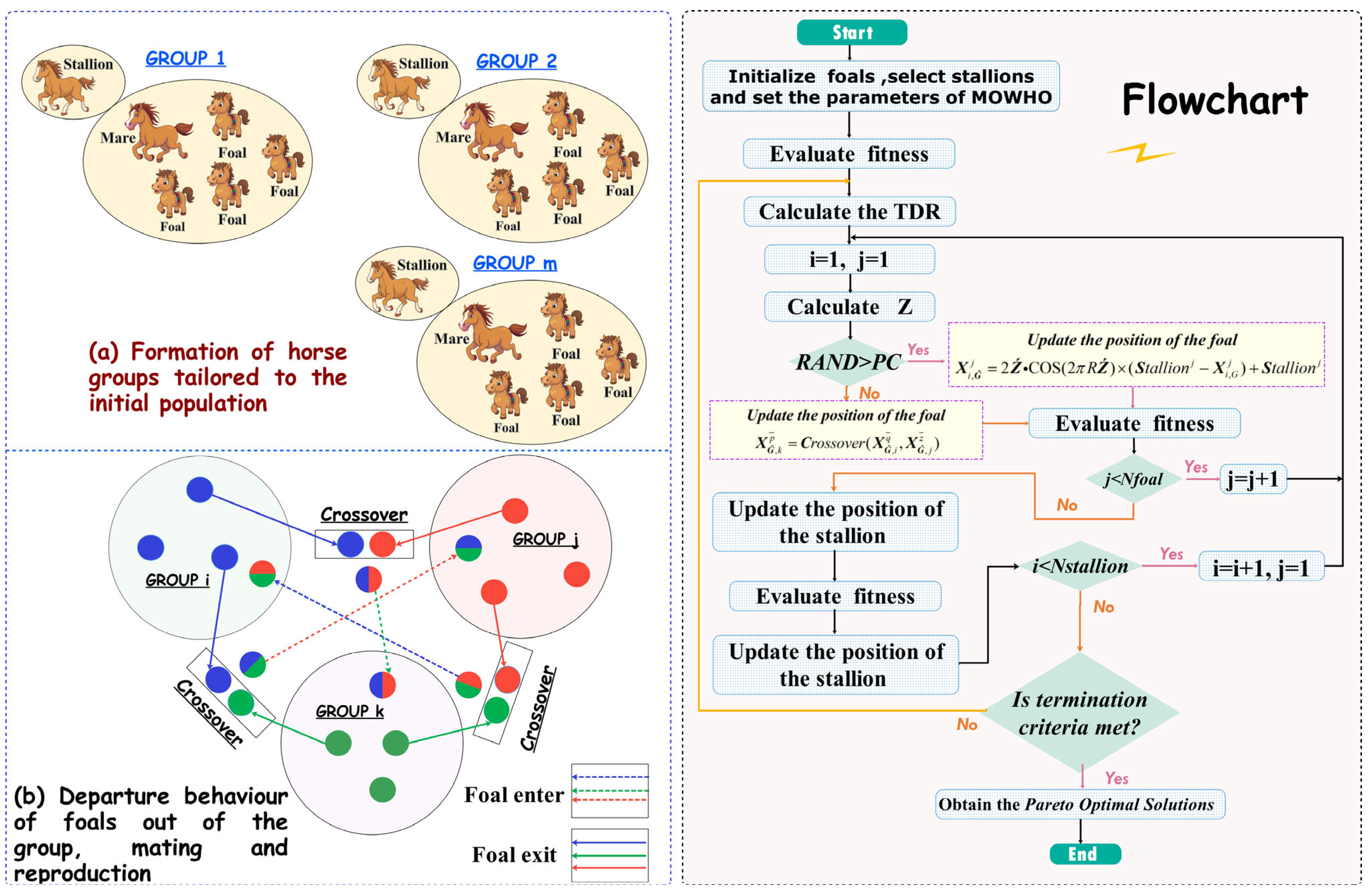
The living behavior of stallions, several mares, and foals in the wild horse society inspired the wild horse optimization algorithm (WHO) [38]. The decency behavior of horses, such as grazing, chasing, dominance, leadership, and mating, has been used to construct a new method. In comparison to other intelligence algorithms, the optimization process of horses departing from the group and mating with horses from other groups efficiently avoids the algorithm slipping into local optimization and balances the algorithm’s exploration and development. On this basis, this paper introduces the concepts of the Pareto optimal solution and external archiving mechanism into WHO and creatively proposes a multi-objective wild horse swarm optimization algorithm (MOWHO) to solve complex forecasting problems. Figure 1 illustrates the key link and the flowchart of the algorithm.
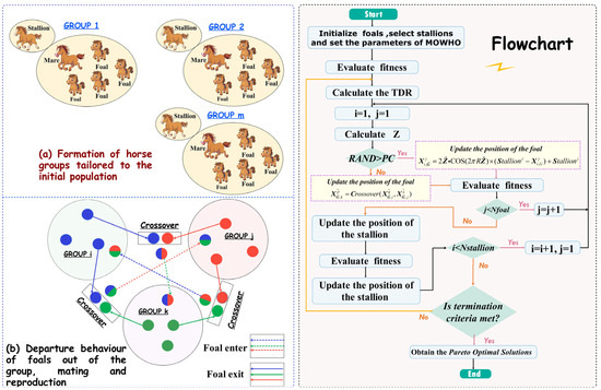
Figure 1.
Key link and the flowchart of MOWHO.
- (1)
- Creating an initial population.
An initialized random population is constructed and determines the objective value . Then, the groups are divided. Let the population size be ; then, the number of groups is , where indicates the proportion of stallions. The remaining populations are divided equally into these groups according to the number of stallions, (Leader). Figure 1a shows an example of this population division.
- (2)
- Grazing behavior.
The algorithm positions the stallion as the central point of the grazing area, with group members moving and searching around the ’s perimeter by , where is the position of the mare and foal and is an adaptive mechanism: . is a uniform random number. The COS function enables the population to move in a 360-degree direction. The index satisfies the condition and this results in and , where TDR is the parameter regulator by , which gradually decreases to 0 with the number of iterations.
- (3)
- Improved nonlinear update strategy.
To overcome the shortage of the only local search, a new nonlinear was proposed by , where is a random number. Through the nonlinear updating mode, the algorithm performs global and local searches in the whole iterative process. Therefore, in the paper.
- (4)
- Horse mating behavior.
Horses have unique forms of decent behavior, i.e., the foal will leave the original population when it is about to mature, the male horse will join the single horse group, and the female horse will join another family group. Such decent behavior avoids inbreeding among horses. WHO uses the mean crossover operator to simulate this behavior in horses: , where is the distance from group k; and are two maturing foals from i group and j group, respectively. Figure 1b shows this mating and departure behavior.
- (5)
- Group leadership.
Each group has a leader () who leads the group to occupy the water hole and occupy a dominant position. ( is the current optimal solution).
where and are the next and current positions of the leader of the i group. In addition, for the selection of leaders, , in each group, we randomly select leaders in the initial stage to maintain the diversity of algorithms. In the later stage, the position of the leader is exchanged in the group according to the Pareto dominance relationship.
- (6)
- Adaptive T-distribution variation strategy.
The variation operator in the algorithm uses the T-distribution with the number of iterations (Iter) serving as the degree of freedom. This aims to balance exploration and development by . The probability density function is as follows:
where is the Gamma function.
- (7)
- Multi-objective version introduction.
This paper innovatively introduces the Pareto optimal solution , and external Archiving mechanism into WHO, and constructs a multi-objective wild horse optimization algorithm (MOWHO) suitable for time-series forecasts. In the current iteration, serves primarily as a repository for the non-dominated solution , thus establishing an upper limit . Upon acquiring a new non-dominated solution via the iterative method, it undergoes comparison with the archived member . If , , it shall incorporate in . To refine , the optimization algorithm will retain the superior solution within while discarding the least effective one. The selection of the most advantageous starting point for the subsequent iteration is conducted through the application of a roulette-based mechanism , where is considered a constant, while represents the number of solutions that are closely related to the i solution. assigns higher weights to solutions located in regions with fewer samples at the Pareto optimality boundary. This strategy aims to expand the coverage to provide a more diverse and comprehensive solution. It is worth noting that the two optimization objectives and constraints of this study are as follows: and .
3. The Main Structure
The principal architecture is depicted in Figure 2, with the specific workflow delineated as follows. Initially, trend decomposition techniques are employed to extract trends, seasonal, and irregular components from raw electricity price data. Subsequently, the three most accurate forecasting models are selected for multiple simulations and parameter adjustments to ensure the stability of results. Ultimately, the multi-objective optimization algorithm is utilized to execute a weighted combination of the three models. And the comparative results are obtained by analyzing the error evaluation indexes.
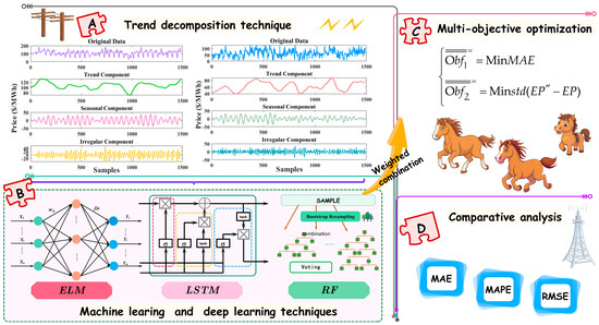
Figure 2.
The main structure of this study.
4. Case Study and Evaluations
4.1. Datasets and Preprocessing
In this comparative analysis, we leveraged datasets derived from authentic electricity markets. The Singapore electricity market (SGP-EP), inaugurated in 2003, represents Asia’s pioneering deregulated market. Recent years have seen the Singaporean government adapt to the global movement towards energy transition, enacting long-term strategies for the decarbonization of its electricity sector. This initiative has culminated in the development of a sophisticated framework for electricity generation and retailing. Conversely, the Australian National Electricity Market (AUS-EP), initiated in 1998, extends over 5000 km, making it the world’s most extensive alternating current electricity system. Characterized by its leading position in global price volatility, it ranks among the most unstable electricity markets internationally.
In the context of electricity markets, the data on electricity prices exhibit pronounced volatility and are frequently characterized by a surplus of peak values. Utilizing unadjusted electricity price series as inputs for predictive models inherently compromises the precision of future price forecasts. To mitigate this challenge, our approach encompasses the identification and subsequent adjustment of aberrant outlier data points. For example, within the Singaporean electricity market, outliers are ascertained utilizing the 3σ criterion. Conversely, the Australian market’s outlier data, distinguished by their considerable deviation resulting in atypical standard deviations, necessitates outlier identification through box plot analysis. Following outlier adjustment, data imputation is conducted employing the piecewise cubic Hermite interpolation polynomial (PCHIP) method. It aims to approximate the original data by a series of cubic polynomials, each of which is responsible for interpolating between two points in the dataset. The polynomial is expressed as follows: , where , are the positions of the two neighboring points of the point to be interpolated, , , , corresponds to the dependent variables of the independent variable , , and , are the corresponding derivatives. This methodology ensures the interpolation curve’s monotonicity and smoothness, effectively eliminating the introduction of supplementary local extrema. Such a feature renders it exceptionally applicable to contexts necessitating the mitigation of undue oscillations and the retention of inherent data trends and attributes.
Our dataset encompasses 31 days from 1 January to 31 January 2024 (sample interval: 15 min). We adopted a stratified split for each dataset into training, validation, and test sets in a 6:2:2 ratio, ensuring rigorous methodology and comprehensive analysis. The specific features of the datasets are shown in Table 2.
Table 2.
Statistical features of the datasets.
4.2. Evaluation Metrics
In assessing the predictive model, three essential metrics were utilized: the Mean Absolute Error (MAE), Mean Absolute Percentage Error (MAPE), and Root Mean Square Error (RMSE) [39,40]. The equation and indicator strengths are shown in Table 3.
Table 3.
Three indicators.
4.3. Experimental Setup
In this segment, we test the proposed hybrid short-term electricity price forecast (HSEPF) model through experimental studies. We begin by outlining the model’s complex operational settings, followed by a thorough examination of the results obtained from these processes. The first case demonstrates the model’s significant ability to integrate various forecasting elements, showing a clear advantage over traditional methods. The second case highlights an improvement in performance compared to models based on different decomposition techniques. The third case emphasizes the model’s exceptional accuracy in predictions thanks to its novel approach of intelligently weighting multi-objectives.
4.3.1. Operational Settings
In the field of deep learning, model parameters play a pivotal role in determining both the computational efficiency and the accuracy of experimental simulations. This study has rigorously tested these parameters across a series of simulation experiments, with the definitive configurations enumerated in Table 4.
Table 4.
Parameter settings.
4.3.2. Case I: Comparison with Predictive Classical Models
Case I involved conducting a comparative experiment with a single model. In this scenario, ARIMA, BP, ELM, LSTM, and RF single models were first used for direct prediction. Subsequently, considering that combining multiple models would increase the complexity of the prediction framework, this paper intended to use the three best-performing single models for decomposition-ensemble [41]. The prediction results are shown in Table 5.
Table 5.
Results of the compared models for different markets.
(a) For AUS-EP forecasting, the developed HSEFP system was evaluated alongside five benchmark models. This comparison provides a fundamental insight into the advanced capabilities of the proposed system. Specifically, when making a 1-step prediction—which involves forecasting the upcoming half-hour—the HSEFP system demonstrates superior performance with parameter settings of = 2000, = 5, = 3, = 100, and = 100. It achieved = 7.3362, = 14.9100%, and = 9.7486. In contrast, the benchmarks reported MAE values above 10, MAPE values ranging from 22% to 27%, and RMSE values exceeding 15. The prediction accuracies are significantly better relative to all the base single models. Figure 3 shows the forecast trends and error indicators of each model.
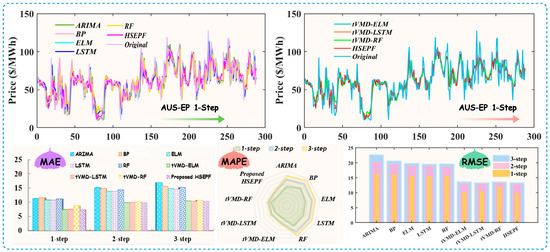
Figure 3.
The forecasting performances in Case I for the AUS market.
(b) For SGP-EP forecasting, the overall forecast error was smaller because this market is more stable than the AUS-EP. When 1-step forecasting was performed, the best forecasting performance in the benchmark model was ELM, with parameters = 5, = 15, = 1, and = sigmoid resulting in = 5.9693, = 6.0769%, and = 9.3607. HSEFP has a better forecasting performance (with parameters = 100, = 100, = 15, = sigmoid, = 150, = 500, = 50, and = 5), where the prediction is expressed as = 4.2784, = 4.1918%, and = 5.9268. There is still a gap in the forecasting effectiveness of the single model.
(c) To compare the capability of the data decomposition–integration strategy, the three models ELM, LSTM, and RF, which performed better in the benchmark model, were trend decomposed, and each trend variable was predicted individually. As shown in Table 5, the prediction accuracy improved after integration. From the forecasting results for the AUS-EP, to ensure objectivity in the model comparisons, the ELM was unified with parameters = 5, = 15, = 1, and = sigmoid; the changes in the indicators at 1-step prediction were = {10.8203→7.3713}, = {22.6797%→15.3919%}, and = {15.4311→9.9353}. The LSTM uniform parameters were = 150, = 2, and = 500; the changes in the indicators at one-step prediction were as follows: = {10.7900→7.5255}, = {22.5088%→15.6030%}, and = {15.4000→9.8997}. The RF model unification parameters were = 50 and = 5; the changes in the indicators were = {11.1553→8.8530}, = {24.9916%→18.8079%}, and = {15.4319→11.8251}. From the performance of the metrics, the tVMD decomposition technique effectively improved the accuracy prediction. In the multi-step simulation results, it seemed that 88.89% of the indicators could reflect the superiority of the HSEPF system.
(d) The fitting effect of the SGP-EP models was satisfactory. Additionally, decomposing the model using tVMD significantly enhanced the performance. Under the parameters = 5, = 15, = 1, and = sigmoid, there were = {5.9693→4.3112}, = {6.0769%→4.2667%}, and = {9.3607→5.9489}. The LSTM uniform parameters were = 5, = 150, = 1, = 2, and = 500; the results were = {6.0180→4.5092}, = {6.0780%→4.4401%}, and = {9.4193→6.2313}. The errors of the RF model were reduced (parameters were = 50 and = 5) and the results were = {6.3716→5.4662}, = {6.2949%→5.5410%}, and = {9.4881→7.3617}. The prediction errors all decreased significantly, indicating that the introduction of the tVMD decomposition technique significantly enhanced the hybrid model.
Remark 1.
The effectiveness of the HSEPF system in predicting future electricity prices was validated through experimental results. This system surpassed other single models in forecasting accuracy, as evidenced by the results that support the validity and effectiveness of the proposed modeling theory and methodology. Additionally, the use of the tVMD decomposition technique significantly improved forecasting accuracy. Crucially, this method supports automatic adjustments based on incoming data, enhancing their applicability across various forecasting domains and its practical implementation.
4.3.3. Case ΙΙ: Comparison with Other Data Decomposition Methods
This experiment validated the ability of the tVMD method proposed in this paper to decompose trends in electricity price data, comparing it with the following three models: one without decomposition and two with other varieties of decomposition methods (EMD and EEMD models). The research results for the AUS-EP and SGP-EP markets are summarized in Table 6 and Figure 4, with specific comparative analyses as follows.
Table 6.
Results of the compared models for data decomposition methods.

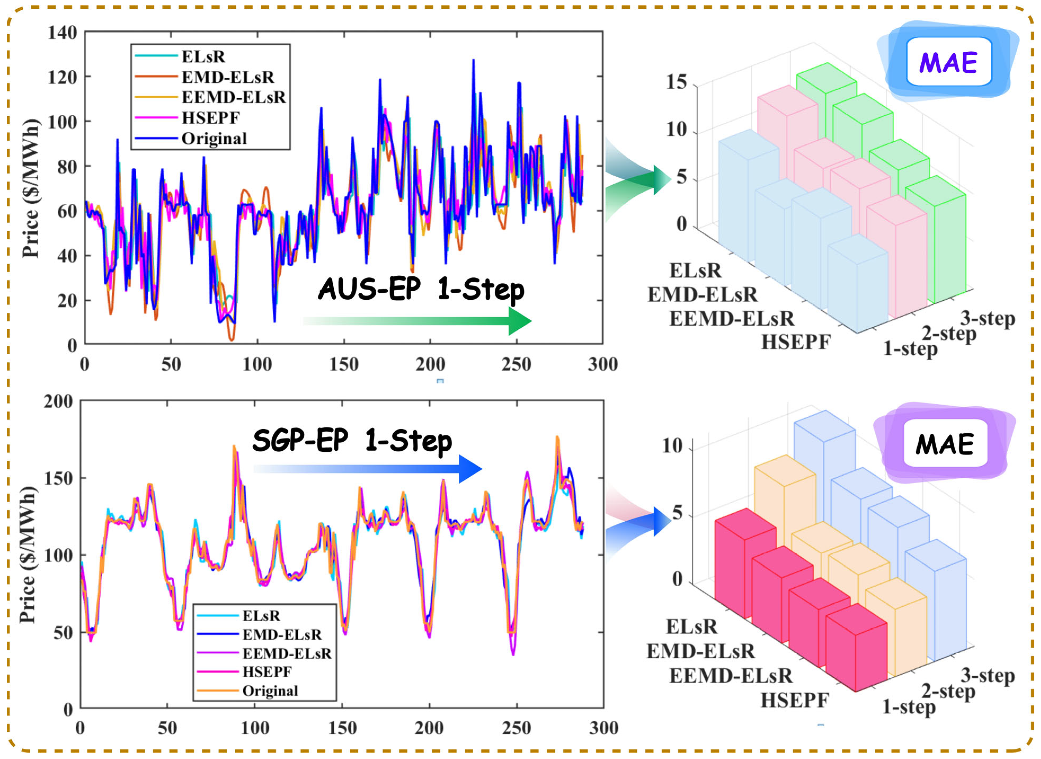
Figure 4.
The forecasting performances in Case ΙΙ.
(a) Due to various uncertainties in the electricity market, electricity price series are typical examples of nonlinear and non-stationary data. Decomposition techniques can significantly improve predictive performance. For the AUS-EP, which is characterized by significant price fluctuations, the multi-step forecasting results of a combined deep learning and machine learning approach without data decomposition are = {10.7941, 13.8730, 14.6527}, = {22.4224%, 31.1126%, 34.2981%}, and = {15.3988, 18.7547, 19.3794}. And for the relatively stable SGP-EP, the combined model ELsR without data decomposition processing can obtain = {5.8931, 8.7458, 10.9286}, = {5.8611%, 8.7855%, 11.0888%}, and = {9.0542, 12.3424, 14.7562} in the calculation of error indicators for multi-step prediction. However, the use of decomposition techniques in the forecasting model reduces the MAPE, MAE, and RMSE values.
(b) For the 1-step forecasting analysis using two market datasets, the accuracy improvements were most pronounced following decomposition through the tVMD method. Notably, there was a significant reduction in all error metrics for the AUS-EP: = 7.5124%, = 5.6502 USD/MWh, and = 3.4579 USD/MWh. In the context of SGP-EP, forecasts derived from tVMD decomposition were most satisfactory, showing improved prediction precision with = 3.12174 USD/MWh, = 1.6693%, and = 1.6147 USD/MWh.
(c) In multi-step forecasting performances across two major market datasets, models decomposed via the tVMD method consistently maintained excellent predictive performance. There are significant improvements in the 2-step and 3-step forecasting accuracy in AUS-EP: = {10.1376%, 12.3727%}. The improvement effects of EEMD and EMD decomposed models are similar in the 2-step, but EEMD performs better at the 3-step, though it still lags behind the proposed HSEFP model by about 3% in terms of the MAPE index. For SGP-EP, the forecasting errors decreased by = {3.8889%, 4.5777%} for 2-step and 3-step forecasting, where the improvement effects of EEMD and EMD were closer.
Remark 2.
Before integration into predictive models, it is crucial to stabilize electricity price data and to adaptively isolate several components that exhibit periodicity. Comparative analyses robustly validate that forecasting precision enhancements afforded by tVMD outperform those achieved with alternative decomposition methodologies. Furthermore, the benefits of this decomposition approach intensify progressively with the increase in forecast steps. The potential of tVMD as a superior tool for improving the reliability and accuracy of forecasting models is underscored by this finding.
4.3.4. Case ΙΙΙ: Comparison with Other Combinatorial Weighting Methods
In this case, we compared the HSEPF model proposed in this paper with a combinatorial weighting strategy based on three different principles. Among them, simple average (SA) weightings were the most common method of model mixing, which reflects the average performance of multiple model combinations. The root mean square (RMS) weighting strategy amplifies large deviations by squaring them and emphasizes the volatility or difference in these values. The multi-objective Dragonfly optimization algorithm (MODA) is widely used in the fields of energy and financial forecasting. Compared with the model prediction results in Table 7, it was found that the HSEPF method achieves higher prediction accuracy and a smaller prediction error. Figure 5 shows the forecast trends and error indicators of each method for the SGP-EP market.
Table 7.
Results of the compared models for other combinatorial weighting methods.
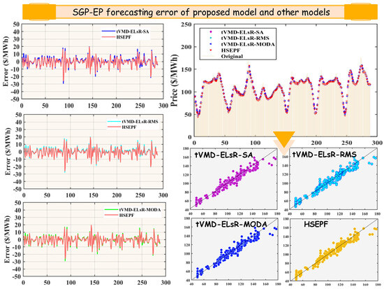
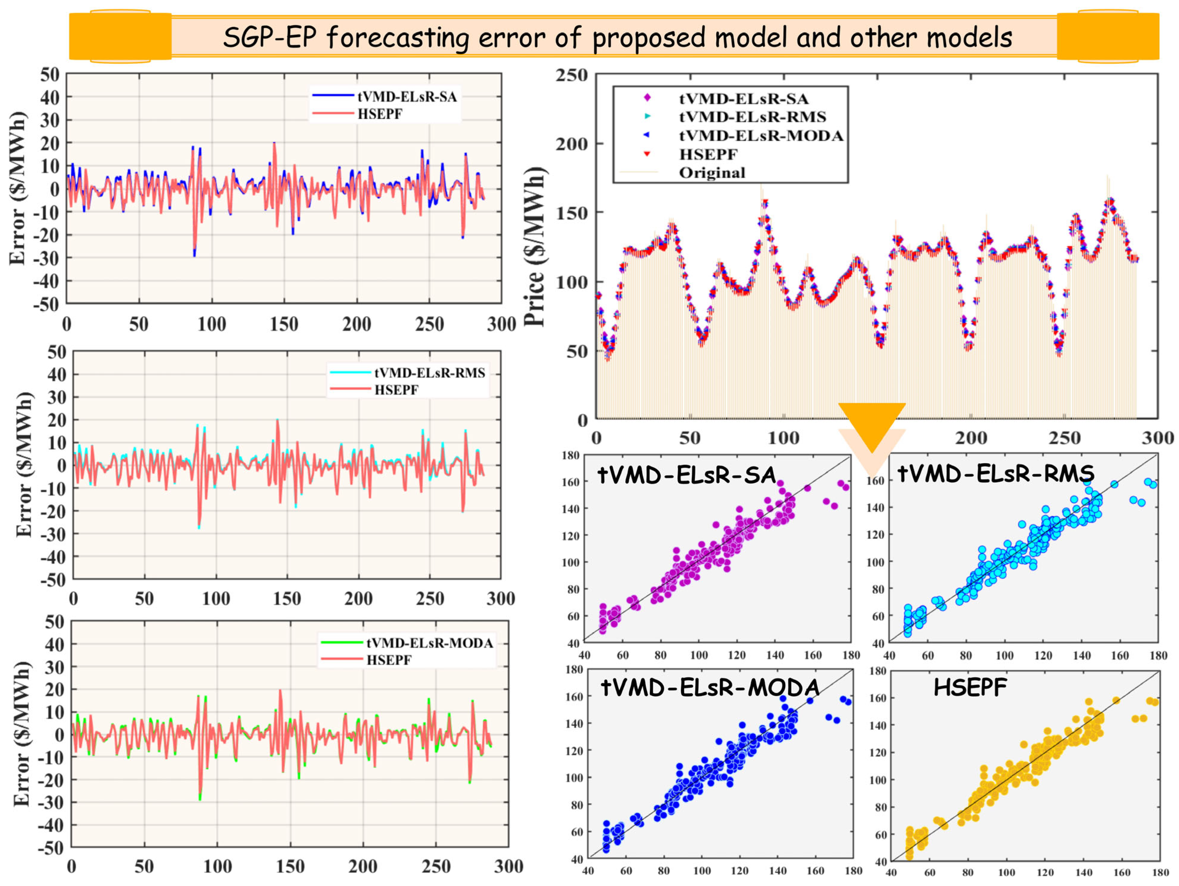
Figure 5.
The forecasting performances in Case ΙΙΙ for the SGP market.
(a) In 1-step forecasting, the HSEPF technique outperformed the other weighting strategies in the forecasting performance in Singapore and Australian markets. tVMD-ELsR-SA, tVMD-ELsR-RMS, and tVMD-ELsR-MODA all performed well when applied to AUS-EP prediction, with tVMD-ELsR-SA being the strategy with the smaller forecasting errors, = 7.7246, = 16.2421%, and = 10.4957. However, there was a gap relative to HSEPF, = 7.3362, = 14.9100%, and = 9.7486. On the other hand, among the comparison models in Singapore, tVMD-ELsR-RMS was the strategy with less prediction error with = 4.4409, = 4.3885%, and = 6.1485. Similarly, the prediction performance lost out to the proposed HSEPF system with = 4.2784, = 4.1918%, and = 5.9268.
(b) In the 2-step prediction of the AUS-EP, the prediction accuracy of the tVMD-ELsR-SA in MAPE index was better: = 20.8713%. At this time, with = 20.9750%, = 9.8568, and = 12.9024, the HSEPF model was slightly better than the tVMD-ELsR-SA model in the performance of MAE and MAPE prediction errors. In SGP-EP, the HSEPF model still maintained a good forecasting ability, where = 5.0703, = 4.8966%, = 6.7367. The overall performance was better than that of the best-performing comparative models: tVMD-ELsR-MODA with = 5.1215, = 4.9873%, and = 6.8570. Therefore, in general, the overall performance of the HSEPF model was better and can be widely used in different electricity price markets.
(c) For a 3-step prediction with a longer prediction period, the HSEPF model had excellent performance in model comparison. In the AUS-EP market, the forecast errors were = 10.2954, = 21.9254%, and = 13.2731. The tVMD-ELsR-SA, tVMD-ELsR-RMS, and tVMD-ELsR-MODA models had closer prediction accuracies, and the MAPE errors were all above 22%. The tVMD-ELsR-RMS model had a better RMSE in the SGP-EP market, which was lower than the HSEPF model with = 0.1586 USD/MWh. However, the HSEPF model of the other two indicators still maintained low prediction errors as = 6.7639, = 6.5111%.
Remark 3.
In this comprehensive study, we substantiated the robust theoretical foundation of the HSEPF model and its superiority in enhancing the predictive accuracy of complex systems. Comparative analyses revealed that other models failed to guarantee stable electricity price forecasts across varied market conditions. In contrast, the model proposed herein consistently demonstrates heightened precision in numerous forecasting scenarios, proficiently responding to the challenges presented by the significant fluctuations in electricity prices.
5. Discussion
To further demonstrate the accuracy of the proposed HSEPF, we perform two additional sets of model tests.
5.1. DM Test
From the comparison of error indicators, we can understand the model prediction performance but cannot discern whether the model is statistically significant or not. The Diebold–Mariano (DM) test can solve this problem, where DM applies to the comparison of predictive ability between two or more models [42]. We can assume that the true value is , the two predicted values in the different models are and , respectively, and the prediction errors of the two models are , where . We can assume that the loss associated with prediction i is a function of the prediction error, , and denotes the loss function by . , where is a first-order difference function of the loss function, if and only if = 0, and have the same prediction accuracy, so we construct the null hypothesis and the alternative hypothesis . Here, means that the two prediction models have the same prediction accuracy, and states that the two do not have related prediction accuracies. The DM statistic can be constructed as , where is the mean of , is the overall mean of the loss function, and is the spectral line density function when the loss difference is 0. The expression of is as follows: , where is the order self-covariance of , and the specific functional equation is , where , and are the consistent estimators when the null hypothesis is valid; the DM statistic obeys N(0,1), HSEPF is used as the benchmark model for the DM test, and the other 14 control models are selected for the DM test. Table 8 presents the outcomes of the tests.
Table 8.
DM test results.
(a) In the comparison of single-mode models, whether for 1-step, 2-step, or 3-step predictions, the results uniformly achieved statistical significance at the 1% level. This outcome indicates a disparity in predictive capabilities between the proposed hybrid system and single models. Further analysis revealed that the predictive strength of models diminishes as the forward prediction steps increase. Moreover, the DM test values exhibited an increasing trend in 85% of the cases. This trend signifies that in 85% of instances, the decline in the predictive ability of single models is notably more pronounced than that of the HSEPF model, underscoring the superior multi-step forecasting stability of the hybrid model.
(b) In the comparison of machine learning models decomposed by tVMD, undecomposed deep learning integration models, and hybrid deep learning models based on other data decomposition techniques, it was found that there were cases where individual models performed better in prediction, but the prediction performance was not stable in multi-step prediction. Among them, the hybrid model ELsR without data decomposition had the highest DM values: = {7.1362, 8.5006, 8.1303} and = {3.5945, 6.4505, 6.8781}, which are both greater than = 2.576, suggesting that the prediction without data decomposition is the weakest. Further analysis revealed that the decomposition technique helped improve the prediction accuracy, whether it was a single model or a hybrid model. For example, in the 2-step prediction in AUS-EP, tVMD-ELM has = 0.5748, and in the 3-step prediction model, tVMD-LSTM has a statistically non-significant difference with the model proposed in this paper, = 0.1518. It suggests that the forecasting performance of deep learning models, after undergoing trend decomposition through tVMD, closely matches that of the optimal model in specific instances.
(c) In the optimization comparison of different weighting strategies, the DM results in the 1-step prediction for the Australian and Singaporean markets, which both exceed = 2.576, indicating a significant difference between the HSEPF model and others at a 99% confidence level. This suggests the effectiveness of the HSEPF model. In the multi-step prediction performance, the majority of models have DM values exceeding = 1.645, signifying a significant difference between models at a 90% confidence level. The HSEPF model demonstrates a leading advantage in electricity price prediction. These findings underscore the robustness and superiority of the HSEPF model in forecasting electricity prices, positioning them as a valuable tool in the energy market.
Remark 4.
According to the results in Table 8, 90.48% of the models passed the test in the AUS-EP, while 88% of the models passed the test in the SGP-EP. This demonstrates a significant difference between the comparative models, confirming the predictive effectiveness of the HSEPF model.
5.2. Performance Improvement Analysis
In predictive research, the improvement percentage of predictive indicators serves as a crucial metric for assessing the predictive capabilities of models. This is quantified as , where denotes the evaluation metric of the reference model, and signifies the predictive indicator from the composite system developed in this study. quantifies the enhancement in predictive performance, with higher values reflecting the superior predictive accuracy of HSEFP. The comparative outcomes of models in AUS-EP and SGP-EP are summarized in Table 9.
Table 9.
Improvement ratio results (%).
(a) Upon analyzing the results of multi-step forecasting, it was evident that the HSEFP prediction system had significantly improved the accuracy and stability of electricity price forecasting in Australia. Particularly, for the single prediction model, the minimum values of the model average improvement rates were = 30.30%, = 32.78%, and = 33.38%. However, when predicting using the single model after tVMD model decomposition, the model improvement rates were all below 10%, indicating the significant impact of tVMD technology on enhancing model prediction accuracy. The average improvement rates of models decomposed by EMD and EEMD are the minimal values of = 13.68% and = 15.93%, respectively, suggesting that these two decomposition techniques have weaker capabilities in decomposing electricity price sequences compared to the tVMD technology proposed in this study. Among the three different combination weighted models, only exceeded 10%, indicating that the hybrid weighting strategy effectively enhanced model prediction capability, yet the HSEFP proposed in this study still outperformed the other comparative strategies.
(b) The electricity price sequence in Singapore exhibited relative stability, with small prediction errors. However, the improvement in forecast accuracy with the HSEFP model was also significant when considering the enhanced percentage. Compared to ARIMA, the HSEFP model demonstrates a superiority of = 51.10%. In the models decomposed by tVMD, the improvement rates were all above 10%, with = 18.33%, = 22.91%, and = 15.31%, showcasing the excellent predictive performance of the MOWHO-weighted strategy. This finding highlights the capability of tVMD to handle electricity price data, significantly enhancing the predictive accuracy of deep learning algorithms and positioning it as a crucial tool for advancing predictive analytics in the field.
Remark 5.
The improvement in percentage through model enhancement further confirms the predictive ability of the HSEFP system. It validates the significant effect of the tVMD technique in enhancing model prediction accuracy, and compared with other weighting strategies, the MOWHO algorithm has clear advantages, which can be further extended to the analysis of time-series prediction.
6. Conclusions and Future Work
The HSEPF system, introduced in this study, is a novel approach for forecasting short-term electricity prices. Initially, acknowledging the high volatility and irregular movements characteristic of electricity price sequences, the HSEPF system applied a stabilizing transformation to the raw data before forecasting. This involves the adaptive extraction of several feature components with distinct central frequencies. Specifically, this study employed the tVMD technique to isolate the trend, cyclical, and irregular components of the dataset. This approach significantly enhanced the efficiency of feature extraction in the forecasting model. Comparative analysis and discussion provided compelling evidence that the application of tVMD exerts a scalable impact on forecasting accuracy, warranting further exploration and validation in a broader data context.
Subsequently, the model inputs the decomposed sequence components into both linear and nonlinear machine learning models for separate predictions before integrating the results from each component. The final stage involved selecting the top three performing single models and employing the MOWHO model to obtain a weighted amalgamation of their outcomes. The experimental results demonstrated that the proposed HSEPF model was capable of predicting electricity prices across different market types. The forecast results in the Singapore market were as follows: = 4.2784, = 4.1918%, and = 5.9268. Australian market data fluctuated dramatically but still obtained smaller errors as follows: = 7.3362, = 14.9100%, and = 9.7486. This system not only enhances prediction accuracy through innovative decomposition and optimization techniques but also demonstrates its universality and effectiveness under different market conditions. This study highlights the potential of combining advanced analytical methods with deep learning models to improve predictive performance in the non-stationary, complex field of electricity price forecasting, providing valuable insights for academia and industry stakeholders.
In future research, two aspects can be explored. Firstly, a generalized and precise electricity price prediction model can be developed by considering various factors, such as user behavior, holidays, and weather. Secondly, future work can focus on peak electricity price prediction based on the current research to achieve higher prediction accuracy.
Author Contributions
Conceptualization, methodology, funding acquisition, supervision, writing—review and editing, H.L.; writing—original draft preparation, data curation, software, validation, visualization, Y.S. All authors have read and agreed to the published version of the manuscript.
Funding
This research was funded by the HSSF of the Chinese Ministry of Education (No. 23YJA790053) and the NSFC (No. 12071302).
Data Availability Statement
The raw data supporting the conclusions of this article will be made available by the authors on request.
Acknowledgments
The authors extend their gratitude to the editors and reviewers for their invaluable comments and suggestions.
Conflicts of Interest
The authors declare that they have no known competing financial interests or personal relationships that could have appeared to influence the work reported in this paper.
References
- Jiang, H.; Dong, Y.; Wang, J. Electricity Price Forecasting Using Quantile Regression Averaging with Nonconvex Regularization. J. Forecast. 2024, 43, 1859–1879. [Google Scholar] [CrossRef]
- Indira, G.; Bhavani, M.; Brinda, R.; Zahira, R. Electricity Load Demand Prediction for Microgrid Energy Management System Using Hybrid Adaptive Barnacle-Mating Optimizer with Artificial Neural Network Algorithm. Energy Technol. 2024, 12, 2301091. [Google Scholar] [CrossRef]
- Iftikhar, H.; Turpo-Chaparro, J.E.; Canas Rodrigues, P.; López-Gonzales, J.L. Forecasting Day-Ahead Electricity Prices for the Italian Electricity Market Using a New Decomposition—Combination Technique. Energies 2023, 16, 6669. [Google Scholar] [CrossRef]
- Tan, Y.Q.; Shen, Y.X.; Yu, X.Y.; Lu, X. Day-Ahead Electricity Price Forecasting Employing a Novel Hybrid Frame of Deep Learning Methods: A Case Study in NSW, Australia. Electr. Power Syst. Res. 2023, 220, 109300. [Google Scholar] [CrossRef]
- Sai, W.; Pan, Z.; Liu, S.; Jiao, Z.; Zhong, Z.; Miao, B.; Chan, S.H. Event-Driven Forecasting of Wholesale Electricity Price and Frequency Regulation Price Using Machine Learning Algorithms. Appl. Energy 2023, 352, 121989. [Google Scholar] [CrossRef]
- Zhang, T.; Tang, Z.; Wu, J.; Du, X.; Chen, K. Short Term Electricity Price Forecasting Using a New Hybrid Model Based on Two-Layer Decomposition Technique and Ensemble Learning. Electr. Power Syst. Res. 2022, 205, 107762. [Google Scholar] [CrossRef]
- Liu, D.; Wei, Y.; Yang, S.; Guan, Z. Electricity Price Forecast Using Combined Models with Adaptive Weights Selected and Errors Calibrated by Hidden Markov Model. Math. Probl. Eng. 2013, 2013, 648101. [Google Scholar] [CrossRef]
- Girish, G.P. Spot Electricity Price Forecasting in Indian Electricity Market Using Autoregressive-GARCH Models. Energy Strategy Rev. 2016, 11–12, 52–57. [Google Scholar] [CrossRef]
- Zhao, Z.; Wang, C.; Nokleby, M.; Miller, C.J. Improving Short-Term Electricity Price Forecasting Using Day-Ahead LMP with ARIMA Models. In Proceedings of the 2017 IEEE Power & Energy Society General Meeting, Chicago, IL, USA, 16–20 July 2017; pp. 1–5. [Google Scholar]
- Imani, M.H.; Bompard, E.; Colella, P.; Huang, T. Forecasting Electricity Price in Different Time Horizons: An Application to the Italian Electricity Market. IEEE Trans. Ind. Appl. 2021, 57, 5726–5736. [Google Scholar] [CrossRef]
- Singh, A.; Sahay, K.B. Short-Term Demand Forecasting by Using ANN Algorithms. In Proceedings of the 2018 International Electrical Engineering Congress, Krabi, Thailand, 7–9 March 2018; pp. 1–4. [Google Scholar] [CrossRef]
- Wu, S.; He, L.; Zhang, Z.; Du, Y. Forecast of Short-Term Electricity Price Based on Data Analysis. Math. Probl. Eng. 2021, 2021, 6637183. [Google Scholar] [CrossRef]
- Wang, P.; Xu, K.; Ding, Z.; Du, Y.; Liu, W.; Sun, B.; Zhu, Z.; Tang, H. An Online Electricity Market Price Forecasting Method Via Random Forest. IEEE Trans. Ind. Appl. 2022, 58, 7013–7021. [Google Scholar] [CrossRef]
- Huang, S.; Shi, J.; Wang, B.; Lyu, J.; Nie, N.; Dong, X.; Li, H.; Zhang, S.; Ren, X. A Meta-Learning Based Method for Day Ahead Electricity Price Forecasting in Markets with Renewable Energy Resources. In Proceedings of the 2023 IEEE 12th Global Conference on Consumer Electronics, Nara, Japan, 10–13 October 2023; pp. 288–290. [Google Scholar] [CrossRef]
- Rezaei, N.; Rajabi, R.; Estebsari, A. Electricity Price Forecasting Model Based on Gated Recurrent Units. In Proceedings of the 2022 IEEE International Conference on Environment and Electrical Engineering and 2022 IEEE Industrial and Commercial Power Systems Europe, Prague, Czech Republic, 28 June–1 July 2022; pp. 1–5. [Google Scholar] [CrossRef]
- Wang, B.; Wei, W.; Su, W. Short-Term Electricity Price Forecasting Based on Data Mining. In Proceedings of the 2022 2nd International Conference on Algorithms, High Performance Computing and Artificial Intelligence, Guangzhou, China, 21–23 October 2022; pp. 394–397. [Google Scholar] [CrossRef]
- Yorat, E.; Ozbek, N.S.; Zor, K.; Saribulut, L. Day-Ahead Electricity Price Forecasting Using Artificial Intelligence-Based Algorithms. In Proceedings of the 2023 International Conference on Innovation and Intelligence for Informatics, Computing, and Technologies, Sakheer, Bahrain, 20–21 November 2023; pp. 121–126. [Google Scholar] [CrossRef]
- Xu, H.; Hu, F.; Liang, X.; Gunmi, M.A. Attention Mechanism Multi-Size Depthwise Convolutional Long Short-Term Memory Neural Network for Forecasting Real-Time Electricity Prices. IEEE Trans. Power Syst. 2024, 39, 6277–6289. [Google Scholar] [CrossRef]
- Yang, W.; Sun, S.; Hao, Y.; Wang, S. A Novel Machine Learning-Based Electricity Price Forecasting Model Based on Optimal Model Selection Strategy. Energy 2022, 238, 121989. [Google Scholar] [CrossRef]
- Bozlak, Ç.B.; Yaşar, C.F. An Optimized Deep Learning Approach for Forecasting Day-Ahead Electricity Prices. Electr. Power Syst. Res. 2024, 229, 110129. [Google Scholar] [CrossRef]
- Najafi, A.; Homaee, O.; Jasinski, M.; Golshan, M.; Leonowicz, Z. Application of Extreme Learning Machine-Autoencoder to Medium Term Electricity Price Forecasting. In Proceedings of the 2022 IEEE International Conference on Environment and Electrical Engineering and 2022 IEEE Industrial and Commercial Power Systems Europe, Prague, Czech Republic, 28 June–1 July 2022; pp. 1–4. [Google Scholar] [CrossRef]
- Qu, Z.; He, L.; Ge, X.; Wang, F.; Xu, F.; Lu, J. A Two-Stage Forecasting Approach for Day-Ahead Electricity Price Based on Improved Wavelet Neural Network with ELM Initialization. IEEE Trans. Ind. Appl. 2024, 60, 5061–5073. [Google Scholar] [CrossRef]
- Wang, J.; Liu, F.; Song, Y.; Zhao, J. A Novel Model: Dynamic Choice Artificial Neural Network (DCANN) for an Electricity Price Forecasting System. Appl. Soft Comput. J. 2016, 48, 281–297. [Google Scholar] [CrossRef]
- Zhang, H.; Hu, W.; Member, S.; Cao, D.; Member, S.; Huang, Q.; Chen, Z.; Blaabjerg, F. A Temporal Convolutional Network Based Hybrid Model of Short-Term Electricity Price Forecasting. CSEE J. Power Energy Syst. 2021, 10, 1119–1130. [Google Scholar] [CrossRef]
- Jiang, P.; Nie, Y.; Wang, J.; Huang, X. Multivariable Short-Term Electricity Price Forecasting Using Artificial Intelligence and Multi-Input Multi-Output Scheme. Energy Econ. 2023, 117, 106471. [Google Scholar] [CrossRef]
- Wang, J.; Yang, W.; Du, P.; Niu, T. Outlier-Robust Hybrid Electricity Price Forecasting Model for Electricity Market Management. J. Clean. Prod. 2020, 249, 119318. [Google Scholar] [CrossRef]
- Zhang, J.; Tan, Z.; Wei, Y. An Adaptive Hybrid Model for Short Term Electricity Price Forecasting. Appl. Energy 2020, 258, 114087. [Google Scholar] [CrossRef]
- Huang, C.J.; Shen, Y.; Chen, Y.H.; Chen, H.C. A Novel Hybrid Deep Neural Network Model for Short-Term Electricity Price Forecasting. Int. J. Energy Res. 2021, 45, 2511–2532. [Google Scholar] [CrossRef]
- Yang, Z.; Ce, L.; Lian, L. Electricity Price Forecasting by a Hybrid Model, Combining Wavelet Transform, ARMA and Kernel-Based Extreme Learning Machine Methods. Appl. Energy 2017, 190, 291–305. [Google Scholar] [CrossRef]
- Zhang, X.; Wang, J.; Gao, Y. A Hybrid Short-Term Electricity Price Forecasting Framework: Cuckoo Search-Based Feature Selection with Singular Spectrum Analysis and SVM. Energy Econ. 2019, 81, 899–913. [Google Scholar] [CrossRef]
- Xu, Y.; Li, J.; Wang, H.; Du, P. A Novel Probabilistic Forecasting System Based on Quantile Combination in Electricity Price. Comput. Ind. Eng. 2024, 187, 109834. [Google Scholar] [CrossRef]
- Yang, W.; Wang, J.; Niu, T.; Du, P. A Novel System for Multi-Step Electricity Price Forecasting for Electricity Market Management. Appl. Soft Comput. J. 2020, 88, 106029. [Google Scholar] [CrossRef]
- Kavakci, G.; Cicekdag, B.; Ertekin, S. Time Series Prediction of Solar Power Generation Using Trend Decomposition. Energy Technol. 2024, 12, 2300914. [Google Scholar] [CrossRef]
- Dragomiretskiy, K.; Zosso, D. Variational Mode Decomposition. IEEE Trans. Signal Process. 2014, 62, 531–544. [Google Scholar] [CrossRef]
- Zhang, C.; Fu, Y.; Gong, L. Short-Term Electricity Price Forecast Using Frequency Analysis and Price Spikes Oversampling. IEEE Trans. Power Syst. 2023, 38, 4739–4751. [Google Scholar] [CrossRef]
- Rockafellar, R.T. A Dual Approach to Solving Nonlinear Programming Problems by Unconstrained Optimization. Math. Program. 1973, 5, 354–373. [Google Scholar] [CrossRef]
- Shi, C.; Wei, B.; Wei, S.; Wang, W.; Liu, H.; Liu, J. A Quantitative Discriminant Method of Elbow Point for the Optimal Number of Clusters in Clustering Algorithm. EURASIP J. Wirel. Commun. Netw. 2021, 2021, 31. [Google Scholar] [CrossRef]
- Naruei, I.; Keynia, F. Wild Horse Optimizer: A New Meta-Heuristic Algorithm for Solving Engineering Optimization Problems; Springer: London, UK, 2022; Volume 38, ISBN 0123456789. [Google Scholar]
- Wang, X.; An, Y.; Wang, J.; Shao, Y. A Novel Prediction-Integration Forecasting System for Short Wind Speed Based on Combined Data Preprocessing Technique and Weight Determination Strategy. Energy Technol. 2024, 12, 2300889. [Google Scholar] [CrossRef]
- Zhang, W.; Kou, M.; Lv, M.; Shao, Y. Improved Combined System and Application to Precipitation Forecasting Model. Alex. Eng. J. 2022, 61, 12739–12757. [Google Scholar] [CrossRef]
- Wang, J.; Guo, H.; Song, A. Photovoltaic Power Combination Prediction System Based on Improved Multi-Objective Optimization Algorithm and Nonlinear Weighting Strategy. Expert Syst. 2023, 40, e13209. [Google Scholar] [CrossRef]
- Diebold, F.X.; Mariano, R.S. Comparing Predictive Accuracy. J. Bus. Econ. Stat. 1995, 13, 253–263. [Google Scholar] [CrossRef]


Disclaimer/Publisher’s Note: The statements, opinions and data contained in all publications are solely those of the individual author(s) and contributor(s) and not of MDPI and/or the editor(s). MDPI and/or the editor(s) disclaim responsibility for any injury to people or property resulting from any ideas, methods, instructions or products referred to in the content. |
© 2024 by the authors. Licensee MDPI, Basel, Switzerland. This article is an open access article distributed under the terms and conditions of the Creative Commons Attribution (CC BY) license (https://creativecommons.org/licenses/by/4.0/).