Abstract
The frequency domain measurement of radiated emissions from electric railways (from 9 kHz up to 150 kHz) has been omitted from the main part of the relevant standard (lack of repeatability and reproducibility of the results is mentioned as the reason). This paper describes the radiated emissions measured from three electric trains to emphasize the importance of the suitable time length selection (by comparing specific durations of the recorded data: 1 min and 5 min) and the influence of calculation methods of the resultant spectrum in frequency domain (RMS, mean, and Max of spectrum). The results revealed the requirement of unique definitions for pre-, during-, and post-measurement factors so that the repeatable and reproducible results could be achieved. The prerequisites for having less uncertain results are as follows: (1) pure background measurement (in energized and de-energized state of the catenary); (2) precoordinated operation mode, speed, and power of the train during the measurement; (3) precise details of the analysis step. A unique analysis method is required (to be clearly elaborated in the relevant standards) to obtain comparable results between different working groups engaged with the radiated-emission measurements from a train in a frequency range of 9 kHz to 150 kHz.
1. Introduction
With the increase in transportation requirement both for people and goods, the enhancement of the electric traction could make some sustainable development goals more achievable. One goal of the International Union of Railways (UIC) is to enhance energy efficiency by 2030 and to decrease carbon emissions per unit of traffic by 50% compared to 1990, and to further improve them by 2050 [1]. The electrification of railway transport is an essential requirement for this. However, the associated electromagnetic emissions potentially have adverse impacts on the performance of equipment [2] and, in some cases, even for personnel and passengers [3].
Generally, electromagnetic emissions are a major challenge in the design of complex electrical systems. The concept of electromagnetic compatibility (EMC) requires more attention both during the design and during the operation of a complicated system. When dealing with systems of large dimensions, especially a mixture of old and modern equipment, the importance of EMC could not be more obvious. In fact, one of the reasons of this problem is that in a complicated large system, there might be different subsystems which are manufactured by various companies so that one subsystem (or more) cannot meet the EMC limits.
The concept of EMC could be addressed from two perspectives:
- To perform a thorough EMC study in the design stage [4]. This method has its own complexities emanating from different causes (e.g., the designed equipment will be installed in an environment that is not always completely determined).
- To consider the concept of EMC as an operational problem that should be addressed after the installation of designed equipment in the real environment.
The hazards of the latter way of dealing with the concept of EMC are clear because an expensive solution might exist. The implementation of which as an afterthought may not be feasible. Therefore, a range of expertise/competence is needed to address EMC [5].
The railway system is one of those complex systems which consists of different types of subsystems (power, communication, control, etc.). Each subsystem could have its own voltage, current, frequency, and specifications. Therefore, the requirement of standardization was incontrovertible to enhance the EMC so that there exist minimum interferences; for instance, setting the switching frequency of the main onboard drive of the train to prevent possible interferences with the railway traffic control [6,7], which comprises a set of various devices and its continuous, reliable operation could be threatened by EMI.
Generally, conductive, induced, electrostatic, and radiated types of EMIs (electromagnetic interferences) have been discussed [8,9,10,11,12] for electric railway power systems. Power quality phenomena such as high-frequency resonant overvoltage have been investigated by some researchers (e.g., [13,14,15]), and it is mentioned that the harmonic overvoltage can cause the substation feeder to trip [16]. Some of the issues emanating from the interferences have been discussed in the literature, such as generated emissions during regenerative braking [17], the influence of induced voltage on conductive structures (e.g., oil and gas pipelines) located near railway lines [18], and the influence of electromagnetic disturbances (from 5 Hz up to 100 kHz) on transport telematics systems and electronic security systems [19].
Emission limits for radiated emissions in the frequency range of 9–150 kHz were specified in IEC 62236-2 (2008) [20]. The frequency range was omitted in later editions due to poor reproducibility of the measurement results. Differences in measurement results as high as 20 dB have been reported for the same train in different places and situations. To have repeatable and reproducible measurement results, additional constraints associated with the operating state of the train, measurement, and ambient conditions need to be specified [21]. Most of the uncertainties of radiated-emission measurement of electric railways have been discussed in [22]. With respect to the progress in power electronic devices in recent decades and regarding the high penetration of this kind of equipment, the importance of the switching frequency is highlighted, which could often range from a couple of kHz up to several hundreds of kHz and even more.
Moreover, the pantograph of traction vehicles (which is a kind of sliding contact) powered by an electric catenary line has a highly non-linear nature [1]. This electric arcing could have some consequences. Among them, the conducted and radiated interferences have higher importance [23]. Research about this discharge process revealed that a faster vertical approaching motion between the pantograph and catenary generates a higher radiation intensity [24]. Moreover, the catenary could be an effective antenna with regard to its length and half of the wavelength of a specific frequency, which would result in longitudinal propagation of the emission [25]. It shows the importance of the lower frequency ranges based on the length of the catenary (considering the distance between neutral sections or the distance between two sections of the catenary, which are fed by different feeders from adjacent substations). The phenomena relevant to the switching transients in electronic converters could be included in this category, which, together with emissions emanated from pantograph arcing, could cause an interference problem with the signaling (track circuits, etc.) and telecommunications of the noisy line [1].
Researchers have conducted different studies on various equipment (e.g., signaling, axle counters, automatic train protection, and trackside video monitoring systems) in railway infrastructure to identify their electromagnetic behavior in different frequency ranges. The Technical Specification for Interoperability (TSI) sets limits on both radiated and conducted emissions and the various signaling system components’ capacity to be immune to such interference [26]. If electromagnetic fields have been considered, the following frequency bands for frequency management regarding compatibility requirements of trackside signaling are specified (for 1435 mm, 1520 mm, 1524 mm 1600 mm, and 1668 mm gauge network): band 1 (27 kHz–52 kHz), band 2 (234 kHz–363 kHz), and band 3 (740 kHz–1250 kHz) [27]. So, the magnetic fields generated by rolling stock can potentially interfere with the operation of train detection systems, and as the focus of this paper is on 9 to 150 kHz, therefore, the frequency range of 27 to 52 kHz is important from the signaling system interference point of view. According to the literature [28], the frequency range in which PLC (power line communication) systems can operate covers frequencies from 125 Hz to 100 MHz (Ultra narrowband, Narrowband, and Broadband).
In [29], the electromagnetic interference for axle counters in parts of the Indonesian railway system for two acceleration and deceleration modes is investigated. They concluded that at lower frequency ranges (10 to 100 kHz), the levels are very close to the standard limit, which could interfere with the axle counters system. In [26], the magnetic field generated at the track level by the traction current was measured in order to assess the EM environment in which the axel counters have to operate in Italy, and they reported the compatibility with the limits. In [30], the significance of the issue of assessing the influence of radiated emissions (emanated from rail vehicle) on the operational process of trackside-video-monitoring systems is noted. Some researchers [31,32] proposed models or programs in order to investigate parts of EMI problems in electric railway traction systems and the axle counter system. Some preventive measures to mitigate the EMI in rolling stock is proposed in [33]. They proposed the permissible limits of currents (for various track circuit frequencies from 4.75 kHz up to 17 kHz) to prevent interference between traction return currents with the frequency-modulated automatic train protection (ATP). Recently, the impact of electromagnetic radiation emanating from railway systems on passengers traveling in a train are studied in [34]. The results showed that the radiation levels were lower than the limits in the International Committee on Non-Ionizing Radiation.
There are other applications (other than railway infrastructure) which emit specific frequency emissions or are sensitive to the emissions in specific range of frequency. For instance, in a frequency range which is called very-low-frequency (VLF) band (3 kHz up to 30 kHz), there are some transmitters (Omega navigational transmitters and Navy communication transmitter) and some equipment (visual display terminals, induction stoves) which could be a source or victim of interferences. It should be mentioned that in the low-frequency (LF) band (30 kHz to 300 kHz), some transmitters (Loran navigational transmitters) exist which should be considered in the EMI context [35]. Moreover, in airports, there are some specific appliances that intentionally or unintentionally (electric-plane-charging stations [36]) emit frequencies in the VLF and LF band that will be important in the case of an electrified railway near an airport.
In signal processing, the time–frequency domain has often been exploited for analyzing signals with fast-changing spectral contents [37,38,39,40,41,42,43,44,45,46]. In this paper, a time-domain-based measurement approach is used. This allows for choosing various analyzing tools in order to make a joint time–frequency analysis and have a better understanding of the dominant frequencies (in the range of 9 kHz to 150 kHz) which are present in the magnetic-field-measured data during train passage. One of the most significant challenges in EMC investigations in the time and time–frequency domain is how to analyze the recorded data and interpret the processed data. After performing the measurements and data collection, based on the device which is used for the measurements and its sampling frequency, the analysis could be conducted regarding the main parameter of interest, the focused frequency range, etc.
If the case of radiated-emission measurement in the frequency range of 9 kHz to 150 kHz is considered, one of the sources of uncertainties might be related to the result analysis stage. If the analysis method is clearly decided and defined in the relevant standards, then there might be more convergence in the outputs of different working groups responsible for the measurement in this specific range of frequency.
The main contributions of this work include the following:
- Evaluating and comparing the radiated emission emanating from freight (with and without carriage) trains and passenger trains in Sweden;
- Emphasizing the importance of the time length of the signal in the time domain and its effect on the extracted frequency domain spectrum;
- Proposing other calculation methods (rms, mean, and max) of the resultant spectrum of radiated emission from different trains in the range of 9 to 150 kHz in order to compare the performance of the trains (as it is a moving source of emissions); and
- Proposing a concept of pure background measurement for future works and also emphasizing the requirement of some prerequisites (pre-, during-, and post-measurement factors), which could enhance the repeatability and reproducibility of the results.
2. Materials and Methods
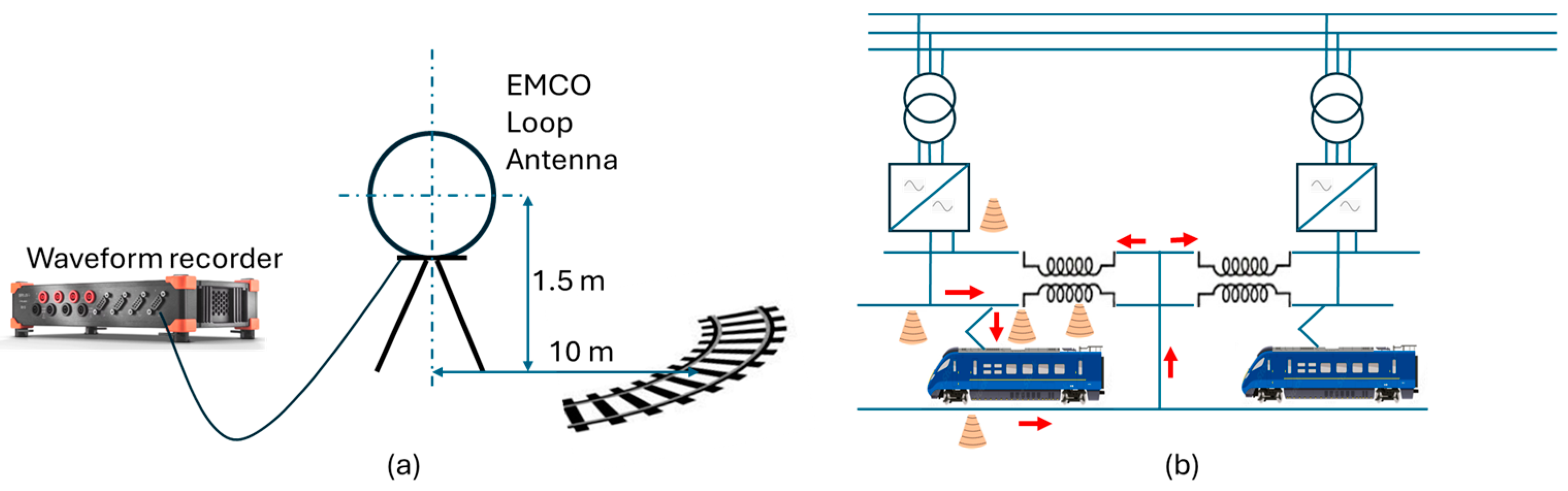
The measurements were taken from passing freight and passenger trains in the north of Sweden in accordance with the procedure outlined in IEC 62236-2 (EN 50121-2) [20]. This has been described in Figure 1a. Figure 1b shows the complex nature of the electromagnetic radiation around a traction system on account of different potential sources of electromagnetic radiation emanating from a traction system. This paper focuses on measurements from a moving train, and hence, the contribution from remotely located installations like the substations and frequency converters therein is not the main focus.
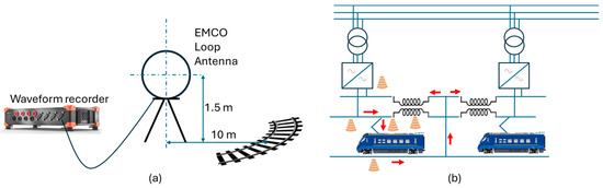
Figure 1.
(a) Measurement setup used for measurement of radiated disturbances in the frequency range (9–150 kHz). (b) Some identified sources of electromagnetic radiation in the traction system. Electromagnetic radiation will also be influenced by auxiliary communication and signaling equipment along the tracks (not shown).
The first and second measurements were taken from freight trains, and the measurement location was in Skellefteå (64°45′14.0″ N, 20°57′07.8″ E) for both of them. In the first measurement, a freight train passing from Bastuträsk to Skelleftehamn was Rd2 type manufactured by ASEA, an electric locomotive operated by Green Cargo, which passed the measurement point around 11:52 on 4 May 2023. The rated power of this model is 3600 kW (4800 hp), but it was a locomotive without any carriages being pulled. In the second measurement, the manufacturer, operator, and destination of the freight train were almost the same as in the first measurement, but it was Rc4 type and loaded with around 30 wagons which passed the measurement point around 15:20 on 10 May 2023.
Measurements from the passenger train were taken at a place (64°45′06.3″ N, 20°02′13.3″ E) which was located at around 4 km south of Bastuträsk. The passenger train was Bombardier Regina X52 electric multiple unit type (9051 Norrtåg) which passed the measurement point around 10:51 toward Vännäs on 22 May 2023. The two cars type of this model has a rated power of 1590 kW (2132 hp). The temperature, weather condition, wind speed, wind direction, and humidity for each measurement are mentioned in Table 1. As identified in IEC 62236-2, the effect of these parameters on radiated-emission measurement is evident but not explicitly studied in this paper.

Table 1.
Information of each measurement.
For this frequency range (9 kHz to 150 kHz), a loop antenna (EMCO ETS-Lindgren Model 6502, frequency range of 10 kHz to 30 MHz) with a diameter of 60 cm (23.6 in) was used.
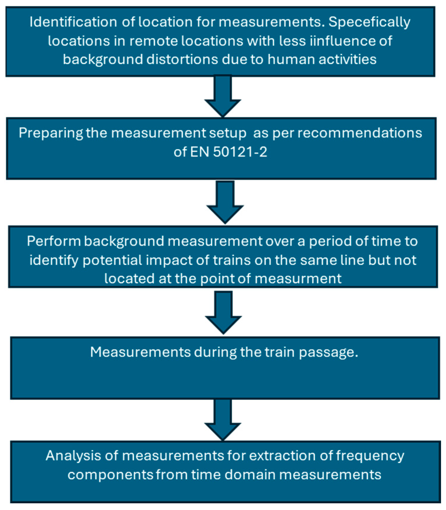
The measurement procedure used during measurements is described in Figure 2. The height and distance of the antenna should be adjusted based on IEC 62236. The height of the center of the antenna was around 1.5 m above the rail level, and the horizontal distance from the center line was 10 m. The DEWESoft (SIRIUS-HS-LVv2-Software Version:2024-1) recorded the output voltage of the loop antenna in time domain with a 500 kHz sampling frequency. Before the arrival of the train to the measurement location vicinity, several backgrounds in the time domain were recorded. Moreover, during the passage of the trains, the measurements were recorded. The output of the antenna is a time-domain AC voltage signal that is measured in volts. By converting to the frequency domain using the STFT function in MATLAB, the energy of the signal can be recorded in dB and by applying the antenna factor to the output voltage of the antenna, the magnetic field signals in dBμA/m) could be calculated. The STFT of the magnetic field signal has been computed with the following parameter settings: resolution bandwidth of 200 Hz, Hanning window function, and 50% overlap.
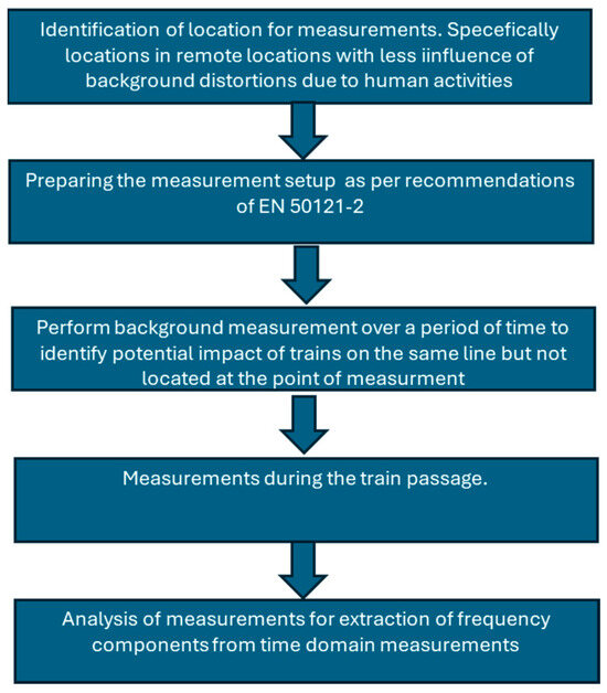
Figure 2.
The measurement setup procedure adhered for the reported results.
Then, a comparison was made between the maximum, RMS, and mean values of STFT in the frequency domain for each measurement using MATLAB (2023 A). The STFT of the whole 5 min of the signal and the 1 min section of the signal have been considered. The 5 min maximum of the spectrum shows a maximum of 150,000,000 (500 kHz × 300 s) values for each 200 Hz frequency step (so that from 9 kHz to 150 kHz, there will be 706 values in the frequency axis). Moreover, 30,000,000 (500 kHz × 60 s) values of the spectrum were considered to find the 1 min maximum of the spectrum for each 200 Hz frequency step. The same procedure has been used for the RMS and mean of the spectrum.
3. Results
The time-domain output voltage (5 min duration) signal of the loop antenna and the frequency analysis (of the whole 5 min of the magnetic field signal and the 1 min section of the magnetic field signal in which train is closest to the antenna location) are illustrated in Figure 3, Figure 4 and Figure 5 for each measurement (A, B, and C). Furthermore, the comparison between different measurement is also presented in Figure 6, Figure 7 and Figure 8.
The passage of the train leads to a high-amplitude voltage at the antenna output waveform in the time domain, which might result from pantograph arcing, high current variable speed drive of the train, etc. The sources of radiated emissions in railway traction [20] could be classified into three types:
- Pure radiated emissions directly generated by the rolling stock (motors, onboard power electronics, pantograph arcing, etc.);
- Conducted emissions generated by the rolling stock and transmitted as REs by the traction line (normally a catenary wire), which radiates toward the equipment; and
- Radiated emissions generated by infrastructures such as substation equipment (e.g., static frequency convertor), high-voltage lines near the railway, improper earthing, etc.
As the measurement location (in Skellefteå) was far from the relevant substation (in Bastuträsk), the share of the third type could be considered in the background emissions.
3.1. Measurement A
This measurement was taken during the passage of a no-load freight train (Rd2 type without any carriages being pulled) from Bastuträsk to Skelleftehamn on 4 May 2023. The antenna output voltage (v) in the time domain is illustrated in Figure 3a, which shows the effect of train passage during the first minute (of the total 5 min of the data) while the other peaks from 3 to 5 min are due to the acceleration behavior of the train operator. Figure 3b shows only 1 min (during train passage) of the 5 min signal. Figure 3c is dedicated to the spectrogram (v) of the 5 min signal for each 1 kHz frequency step. Figure 3d illustrates the spectrogram (v) of the 1 min signal (shown in Figure 3b) for each 200 Hz frequency step. Figure 3c,d explicitly reveal high-amplitude spectrums (almost for all frequencies from 9 kHz to 150 kHz) exactly during the train passage in the first minute of the data (around the 24th second) and some higher-amplitude spectrums around the 21st second (which mostly happens for frequencies below 25 kHz). Furthermore, the influence of the acceleration (not only between the 45th second and 75th second but also between the third and fifth minute) could be observed in the frequency domain that probably shows the switching frequency of the variable speed drive of the train, which is around 24 kHz for train A. On the other hand, the frequency of around 57 kHz is observable during the whole 5 min, which probably is related to the switching frequency of the static converter of the main substation or might result from intermodulation [47] between the switching frequency of the variable speed drive of the train and the switching frequency of the static converter of the main substation.
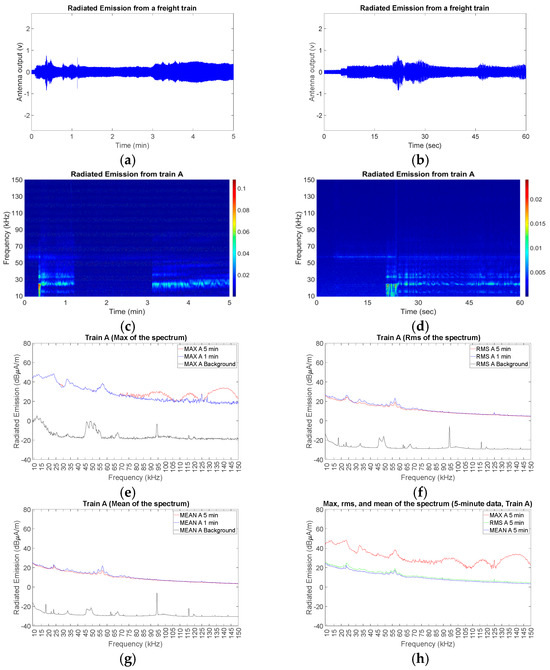
Figure 3.
Measurement results of a no-load freight train (Rd2 type without any carriages being pulled) from Bastuträsk to Skelleftehamn on 4 May 2023: (a) Output voltage of the antenna in time domain for 5 min during train passage from measurement location; (b) same as (a) but for 1 min; (c) spectrogram (v) of 5 min signal shown in (a) for each 1 kHz frequency step; (d) spectrogram (v) of 1 min signal shown in (b) for each 200 Hz frequency step; (e) the maximum of the magnetic field spectrum (dBμA/m) for each 200 Hz frequency step for 5 min, 1 min, and background signals; (f) same as (e), but it shows the RMS of the magnetic field spectrum (dBμA/m); (g) same as (e), but it shows the mean of the magnetic field spectrum (dBμA/m); (h) a comparison between maximum, RMS, and mean of the magnetic field spectrum (dBμA/m) for 5 min signal; all from (c–h) in the frequency range of 9 up to 150 kHz.
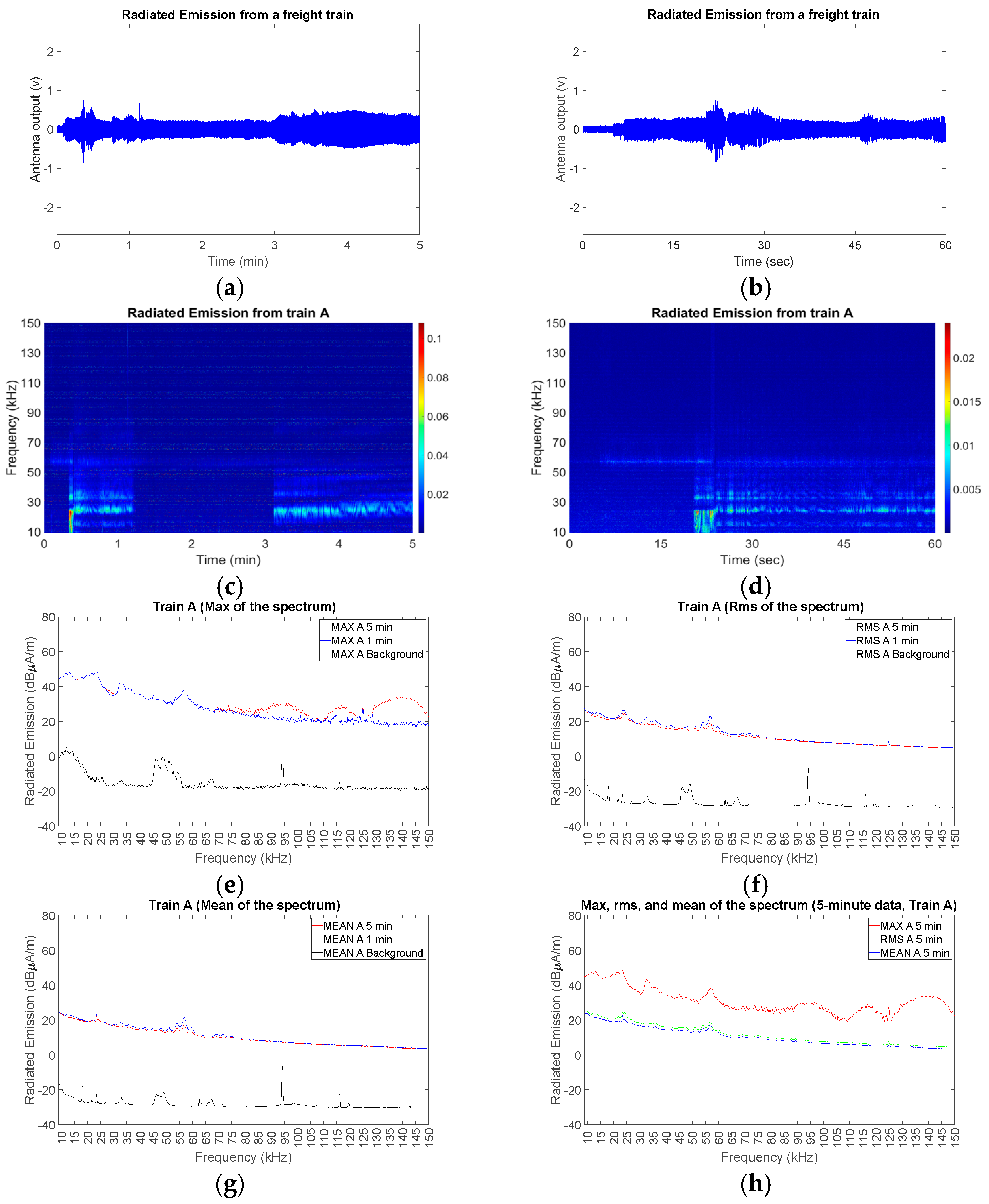
In Figure 3e, the maximum of the magnetic field spectrum (dBμA/m) for (each 200 Hz frequency step for) 5 min, 1 min, and background signals are illustrated in frequency domain. In Figure 3f, the result of 5 min, 1 min, and background of the magnetic field (dBμA/m) data are illustrated in frequency domain so that the RMS of the spectrum for each 200 Hz frequency step is calculated.
In Figure 3g, the result of mean amount of the spectrum of three (5 min, 1 min, and background) magnetic field signals (dBμA/m) are illustrated in frequency domain with 200 Hz frequency resolution. Figure 3h shows a comparison between maximum, RMS, and mean values of the spectrum of 5 min magnetic field signal (dBμA/m) in the frequency range of 9 up to 150 kHz. Figure 3h reveals that in the higher-frequency parts (above 80 kHz), the maximum curve gives a better understanding of the phenomena. The higher-frequency part of the maximum curve (which might result from the effect of the pantograph or the effect of rapid current increment moments (high di/dt) during the acceleration phase) could not be observed in the higher-frequency part of the RMS and mean values (because of the short duration of time in which the train exactly passes the measurement point or the short duration of the acceleration in relation to the whole signal).
On a closer examination of the curves in Figure 3e, the high-frequency behavior could not be seen in the 1 min maximum curve, although it could be observed in the 5 min maximum curve. As just one minute of the time in which the train was closest to the antenna location is considered and as it could be observed from the time-domain figures (Figure 3a,b), the part of the signal which contains the long acceleration phase has not been considered in the 1 min maximum of the spectrum. Therefore, the high-frequency behavior of the 5 min maximum of the spectrum (in Figure 3e) probably could emanate from (high di/dt) in the acceleration phase rather than pantograph arcing.
As is clear, the RMS and mean of the spectrum depend on the number of considered values. In Figure 3f,g, it is illustrated that 1 min curve has higher amplitude than 5 min curve specially in lower parts of the frequency range (below 80 kHz), which shows that, from the RMS and mean points of view, train passage is a kind of lower-frequency phenomena (this train has more emissions in the low-frequency range during the passage from the measurement point). It reveals that those frequency components in the lower part might be emanated from the switching frequency of the train’s variable frequency drive or the switching frequency of the static frequency converters in the main substation (Bastuträsk substation). Moreover, some components such as 12, 13.8, 23.4, 24, 32.6, 36, 54.2, and 57 kHz in Figure 3f,g (both in 5 min and 1 min cases), have higher amplitudes, which shows the steadiness of those frequencies, and it could be concluded that those frequencies might be generated by the supplied current to the train or by the variable frequency drive of the train instead of being generated by pantograph arcing.
Generally, these results are valid for this type of train with this specific operation mode, and it might be different for the other condition.
3.2. Measurement B
This measurement was taken during the passage of a loaded freight train (Rc4 type) from Bastuträsk to Skelleftehamn on 10 May 2023.
The antenna output voltage (v) in the time domain is illustrated in Figure 4a, which shows the effect of train passage between the first and the second minutes (of the total 5 min of the data), while the other peaks from 4 to 5 min are due to the acceleration behavior of the train operator. Figure 4b shows only one minute (during train passage) of the 5 min signal.
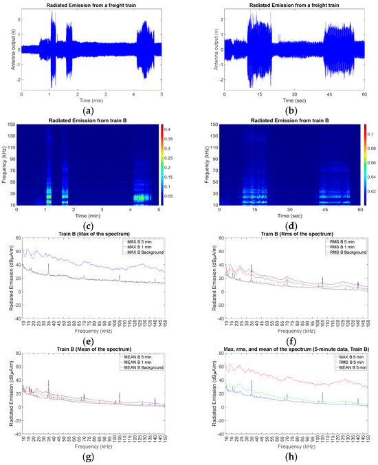
Figure 4.
Measurement results of a loaded freight train (Rc4 type) from Bastuträsk to Skelleftehamn on 10 May 2023: (a) Output voltage of the antenna in time domain for 5 min during train passage from measurement location; (b) same as (a) but for 1 min; (c) spectrogram (v) of 5 min signal shown in (a) for each 1 kHz frequency step; (d) spectrogram (v) of 1 min signal shown in (b) for each 200 Hz frequency step; (e) the maximum of the magnetic field spectrum (dBμA/m) for each 200 Hz frequency step for 5 min, 1 min, and background signals; (f) same as (e) but it shows the RMS of the magnetic field spectrum (dBμA/m); (g) same as (e) but it shows the mean of the magnetic field spectrum (dBμA/m); (h) a comparison between maximum, RMS, and mean of the magnetic field spectrum (dBμA/m) for 5 min signal; all from (c–h) in the frequency range of 9 up to 150 kHz.
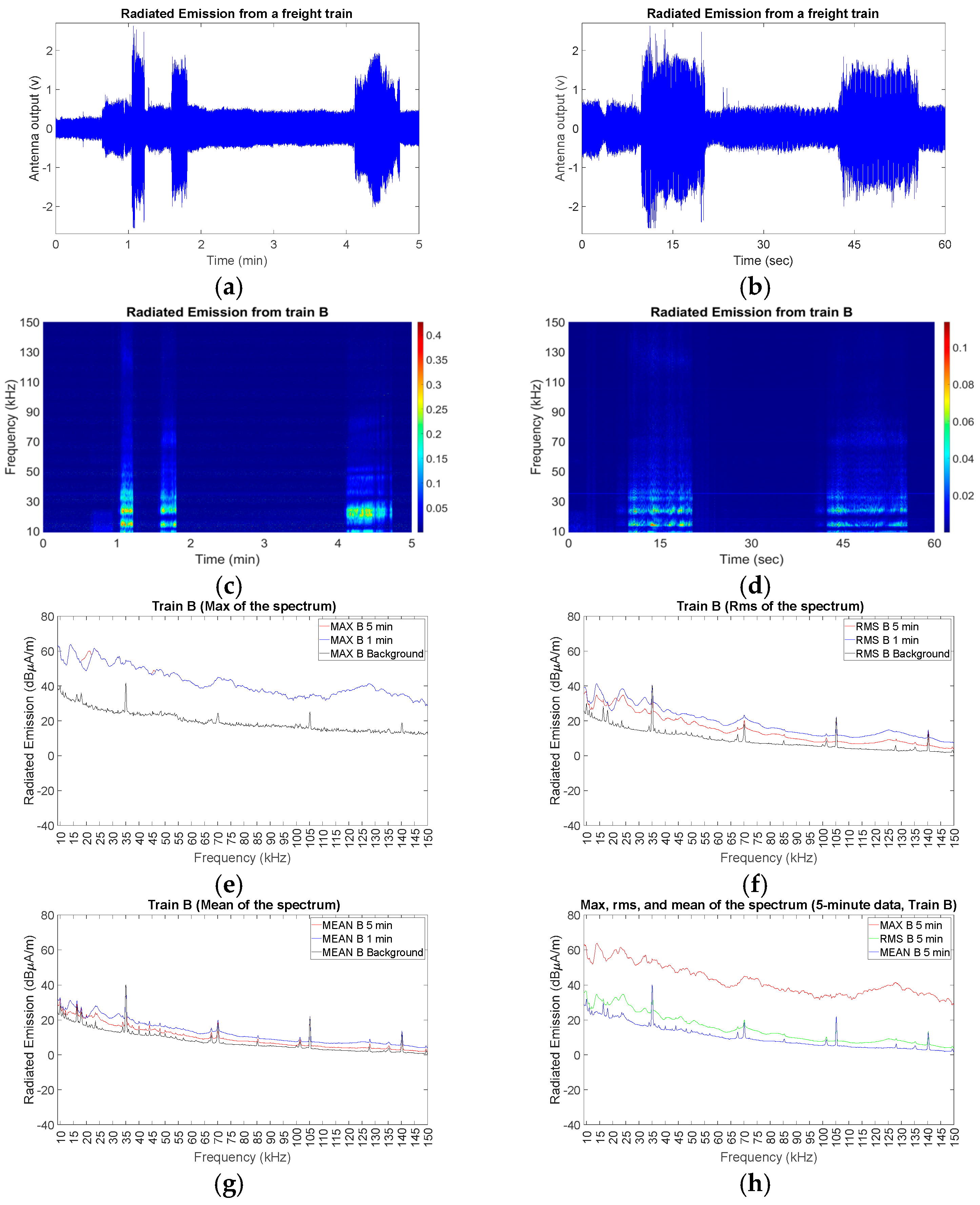
Figure 4c shows the spectrogram (v) of the 5 min signal (shown in Figure 4a) for each 1 kHz frequency step. Figure 4d illustrates the spectrogram (v) of the 1 min signal (shown in Figure 4b) for each 200 Hz frequency step. Figure 4c,d explicitly reveal high-amplitude spectrums (the first one roughly with a 10 s duration almost for all frequencies from 9 kHz to 150 kHz and the second one with a 13 s duration almost for all frequencies from 9 kHz to 90 kHz) exactly during the train passage between the first and the second minutes of the data; and another high-amplitude spectrum (the third one roughly with a 35 s duration for most of the frequencies from 9 kHz to 50 kHz) placed between the fourth and the fifth minutes of the data due to the acceleration of the train. The dominant frequency for the first and second parts of high spectrum are 14.8 and 24 kHz. The effect of pantograph arcing might be observable in the first part at frequencies from 110 kHz to 150 kHz, which could not be detected in the second and third parts of the high spectrums. The dominant frequency for the third part of high spectrum is between 20 and 25 kHz. These three high spectrums probably show that the switching frequency of train’s variable speed drive is between 14 and 25 kHz for train B. On the other hand, the frequency of around 35 kHz is observable during the whole 5 min, which probably is related to the switching frequency of the static converter of the main substation or might result from intermodulation between the switching frequency of train’s variable speed drive and the switching frequency of static converter of the main substation.
In Figure 4e, the maximum of the magnetic field spectrum (dBμA/m) for (each 200 Hz frequency step for) 5 min, 1 min, and background signals are illustrated in frequency domain. In Figure 4f, the result of 5 min, 1 min, and background of the magnetic field (dBμA/m) data are illustrated in frequency domain with the focus on the RMS amount of the spectrum for each 200 Hz frequency step.
In Figure 4g, the result of mean amount of the spectrum of three (5 min, 1 min, and background) magnetic field signals (dBμA/m) are illustrated in frequency domain with 200 Hz frequency resolution. Figure 4h shows a comparison between the maximum, RMS, and mean values of the spectrum of 5 min magnetic field signal (dBμA/m) in frequency range of 9 up to 150 kHz. Figure 4h reveals that in the higher-frequency parts (above 80 kHz), the maximum curve gives better understanding of the phenomena. The higher-frequency part of the maximum curve (might be resulted from the effect of pantograph which) could not be observed in the higher-frequency part of RMS and mean values (because of the short duration of the time in which the train exactly passes the measurement point, this effect will be settled down in the RMS and mean figures).
On examination of the curves in Figure 4e, except for 21.2 and 45.6 kHz, the behavior of the 1 min maximum curve and the 5 min maximum curve are the same. Therefore, the maximum of spectrum of the 1 min data (in Figure 4e) probably could represent almost the worst case of maximum radiated emissions from train B in frequency range of 9 to 150 kHz. As is clear, the RMS and mean of the spectrum depend on the number of considered values. In Figure 4f,g, it is illustrated that the 1 min curve has a higher amplitude than the 5 min curve, especially in lower parts of the frequency range (below 80 kHz), which shows that, from the RMS and mean points of view, train passage is a kind of lower-frequency phenomena (this train has more emissions in the low frequency range during the passage from measurement point). Moreover, it reveals that those frequency components in the lower part might emanate from the switching frequency of the train’s variable frequency drive or the switching frequency of the static frequency converters in the main substation (Bastuträsk substation).
Although for higher frequencies than 105 kHz in RMS curve (Figure 4f), there exists a difference between the 1 min curve and 5 min curve which could emanate from the pantograph arcing, which is a high-frequency phenomenon (this difference could not be detected in mean curves shown in Figure 4g). Moreover, some components, such as 9.4, 13.8, 23.6, 32.2, 35 (which also exist in the background), 40.8, and 54.4 kHz, in Figure 4f (both in 5 min and 1 min cases), have higher amplitudes, which shows the steadiness of those frequencies, and it could be concluded that those frequencies might be generated by the supplied current to the train or by the variable frequency drive of the train instead of being generated by pantograph arcing. Furthermore, some components such as 10, 13.8, 23.4, and 32.2 kHz, in Figure 4g (both in 5 min and 1 min cases), have higher amplitudes, which shows the steadiness of those frequencies; and some other components in Figure 4g with high amplitudes, such as 16.4, 18, and 35 kHz, exist in the background as well. As it is mentioned for train A in a previous subsection, the results in Section 3.2 are valid for this type of train with this specific operation mode (train B), and it might be different for the other condition.
3.3. Measurement C
This measurement was taken during the passage of a passenger train (X52 type) from Bastuträsk to Vännäs on 22 May 2023.
The antenna output voltage (v) in the time domain is illustrated in Figure 5a, which shows the effect of train passage during the first minute (in the first fifteen seconds of the total 5 min of the data), while the other peaks are due to the acceleration behavior of the train operator. Figure 5b shows only one minute (during train passage) of the 5 min signal (that has been illustrated in Figure 5a). Figure 5c is dedicated to the spectrogram (v) of the 5 min signal (shown in Figure 5a) for each 1 kHz frequency step. Figure 5d illustrates the spectrogram (v) of the 1 min signal (shown in Figure 5b) for each 200 Hz frequency step. Figure 5c,d explicitly reveal high-amplitude spectrums (almost for all frequencies from 9 kHz to 150 kHz from fifth to fifteen second) exactly during the train passage during the first minute of the data; and other high-amplitude spectrums (for most of the frequencies from 9 kHz to 40 kHz) due to the acceleration of the train (there is a short period in Figure 5d at around the 40th second which only shows high-frequency content more than 80 kHz that could be emanating from a switching section or neutral section of the catenary or from a switching operation in the main substation). The dominant frequency for the high spectrum during train passage are about 9.8, 17, and 31.6 kHz. The effect of pantograph arcing might be observable in the high spectrum during train passage at frequencies above 50 kHz, which could not be detected in the other parts of the high spectrums. There are three dominant frequency bands (horizontal lines in Figure 5c) for the spectrum of the whole 5 min of the data: 10 to 17 kHz, 20 to 26 kHz, and 30 to 35 kHz.
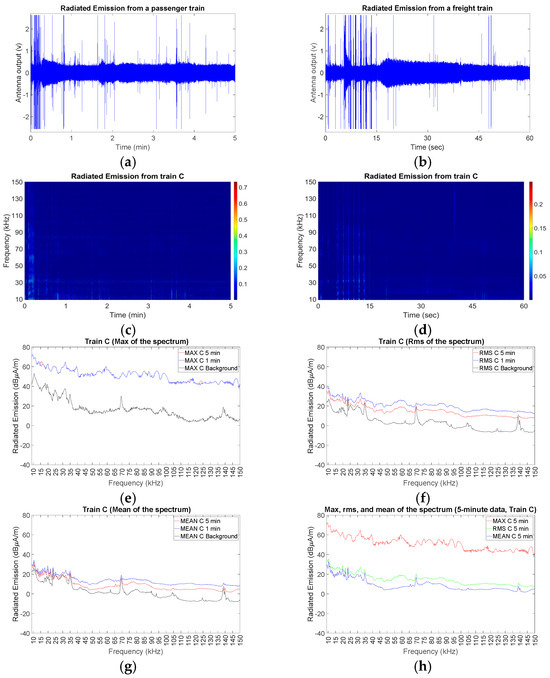
Figure 5.
Measurement results of a passenger train (X52 type) from Bastuträsk to Vännäs on 22 May 2023: (a) Output voltage of the antenna in time domain for 5 min during train passage from measurement location; (b) same as (a) but for 1 min; (c) spectrogram (v) of 5 min signal shown in (a) for each 1 kHz frequency step; (d) spectrogram (v) of 1 min signal shown in (b) for each 200 Hz frequency step; (e) the maximum of the magnetic field spectrum (dBμA/m) for each 200 Hz frequency step for 5 min, 1 min, and background signals; (f) same as (e) but it shows the RMS of the magnetic field spectrum (dBμA/m); (g) same as (e) but it shows the mean of the magnetic field spectrum (dBμA/m); (h) a comparison between maximum, RMS, and mean of the magnetic field spectrum (dBμA/m) for 5 min signal; all from (c–h) in the frequency range of 9 up to 150 kHz.
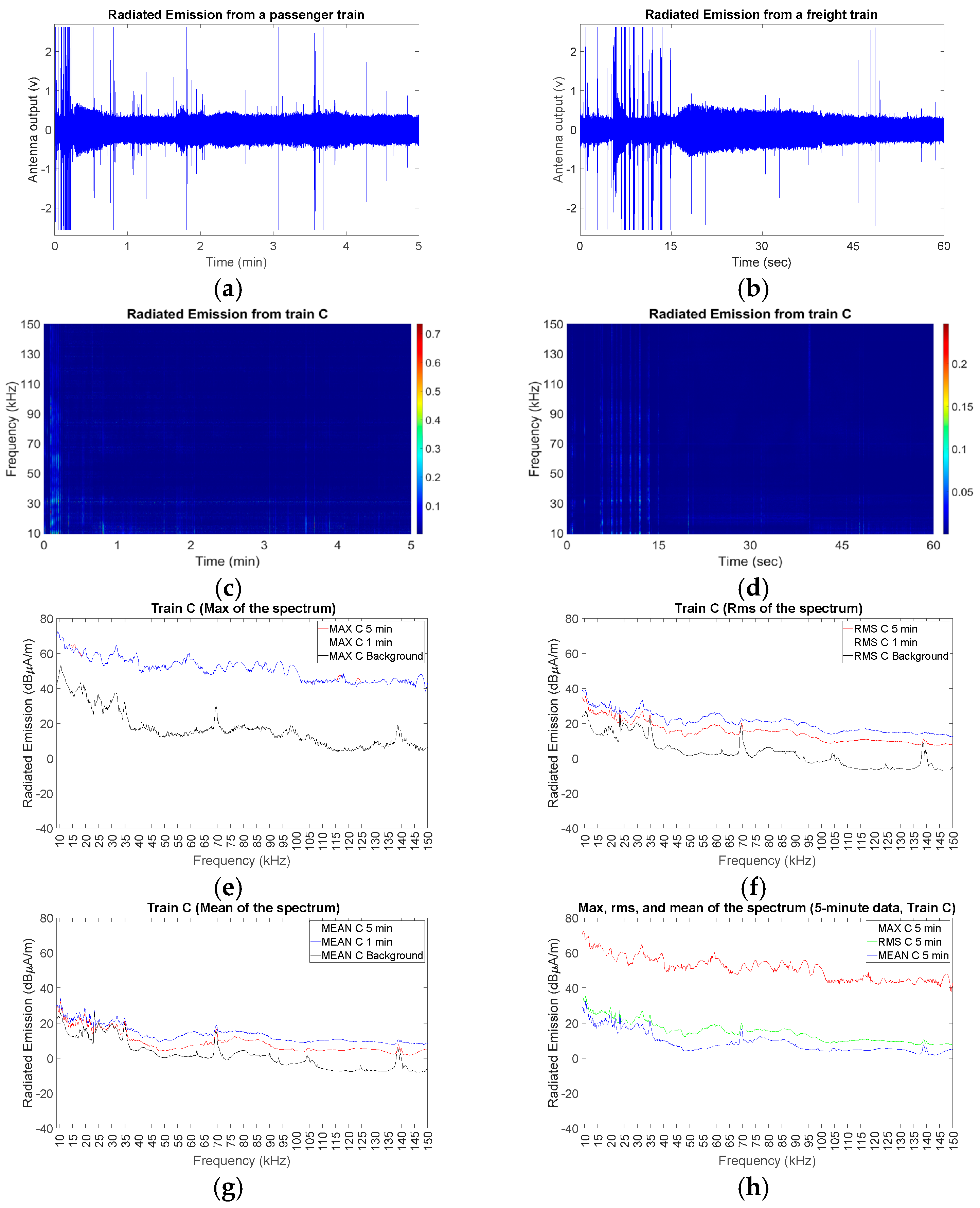
In Figure 5e, the maximum of the magnetic field spectrum (dBμA/m) for (each 200 Hz frequency step for) 5 min, 1 min, and background signals are illustrated in frequency domain. In Figure 5f, the result of 5 min, 1 min, and background of the magnetic field (dBμA/m) data are illustrated in frequency domain, with the focus on the RMS amount of the spectrum for each 200 Hz frequency step.
In Figure 5g, the result of mean amount of the spectrum of three (5 min, 1 min, and background) magnetic field signals (dBμA/m) are illustrated in frequency domain with 200 Hz frequency resolution. Figure 5h shows a comparison between maximum, RMS, and mean values of the spectrum of 5 min magnetic field signal (dBμA/m) in frequency range of 9 up to 150 kHz. Figure 5h reveals that in the higher-frequency parts (above 90 kHz), the maximum curve gives better understanding of the phenomena. The higher-frequency part of the maximum curve (might be resulted from the effect of pantograph which) could not be observed in the higher-frequency part of RMS and mean values (because of short duration of the time that train exactly passes the measurement point, this effect will be settled down in RMS and mean figures).
On examination of the curves in Figure 5e, except for 14.8, 15.8, and 123.6 kHz, the behavior of the 1 min maximum curve and the 5 min maximum curve are the same. Therefore, the maximum of spectrum of the 1 min data (in Figure 5e) probably could represent almost the worst case of maximum radiated emissions from train C in frequency range of 9 to 150 kHz.
As is clear, the RMS and mean of the spectrum depend on the number of considered values. In Figure 5f,g, it is illustrated that the 1 min curve has a higher amplitude than the 5 min curve, especially in lower parts of the frequency range, which shows that, from the RMS and mean points of view, train passage is a kind of lower-frequency phenomena (but the difference in not as much as that of train A and train B because of various accelerations in the whole 5 min by the operator of train C). Moreover, it reveals that those frequency components in the lower part might be emanating from the switching frequency of the train’s variable frequency drive or the switching frequency of the static frequency converters in the main substation (Bastuträsk substation).
Moreover, some components, such as 9, 10.4, 16.4, 23.6, 19.8, 21.6, 23.4 (which also exist in the background), 31.8, and 58.8 kHz, in Figure 5f (both in 5 min and 1 min cases), have higher amplitudes, which shows the steadiness of those frequencies, and it could be concluded that those frequencies might be generated by the supplied current to the train or by the variable frequency drive of the train instead of being generated by pantograph arcing. Furthermore, some components, such as 9.4, 10.4, 11.2, 14.8, 15.6, 16.6, 17.8, 19.6, 21.6, and 32 kHz, in Figure 5g (both in 5 min and 1 min cases), have higher amplitudes, which shows the steadiness of those frequencies; and some other components in Figure 5g with high amplitudes, such as 23.4, 25.2, and 34.8 kHz exist in the background as well. As it is mentioned for train A and train B in previous subsections, the results in Section 3.3 are valid for this type of train (X52) with this specific operation mode (train C), and it might be different for the other condition.
Generally, it could be concluded that a clear definition is needed to be considered in the relevant standards to be able to compare different measurements and consider their effects on various equipment.
3.4. A Comparison between Three Measurements
In this part, it is intended to compare the emissions from three different trains: a no-load freight train (Rd2 type without any carriages being pulled), a loaded freight train (Rc4 type), and a passenger train (X52 type).
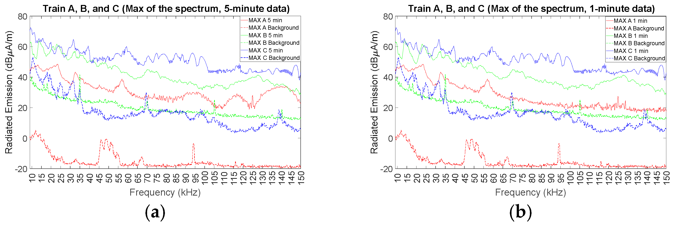
In order to have a better understanding of the effect of the type of the train and other factors on the radiated emission measurements, the maximum of the elements in the spectrum of measured magnetic field from three trains have been compared. Figure 6 shows the maximum in different cases. Figure 6a shows the 5 min maximum curves for three trains and reveals that the no-load freight train (train A without any carriages being pulled) almost in all frequency ranges has lower emissions in comparison with the loaded freight train (train B). Moreover, in most of the frequencies, the passenger train (train C) has higher radiated emissions than the loaded train (train B) and no-load freight train (train A without any carriages being pulled). Furthermore, for the 1 min maximum curves (Figure 6b), which shows the train passage phase, the same observations could be reported. The observations also identify the importance of making the background measurements. The recorded maximum values are reported over differing background conditions and at different independent locations. Therefore, a correlation between the attributes of the locomotive (for example, peak power, electromagnetic shielding designs employed) cannot be made by simply comparing the results. Train A, for example, is anticipated to have the highest power and shows the highest difference between the background emissions and those recorded during the train passage. However, the recorded emission is lower in amplitude than Trains B and C (which have a higher background noise than Train A).
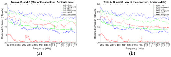
Figure 6.
Measurement results of three different trains in the frequency range of 9 up to 150 kHz: a no-load freight train (Rd2 type without any carriages being pulled) (measurement A: red curve), a loaded freight train (Rc4 type) (measurement B: green curve), and a passenger train (X52 type) (measurement C: blue curve). (a) The maximum of the magnetic field spectrum (dBμA/m) for each 200 Hz frequency step for 5 min and background signals; (b) same as (a) but for 1 min and background signals.
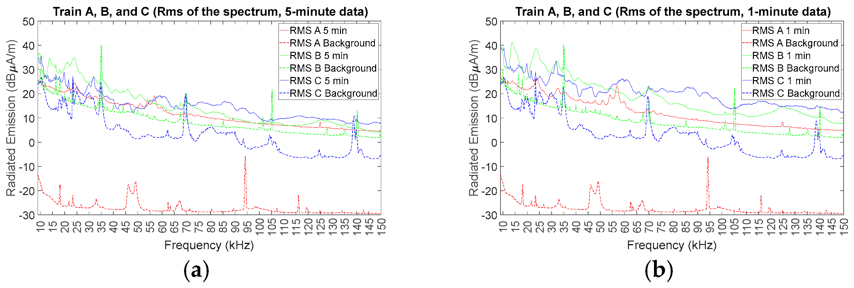
Considering the RMS of the spectral elements of the 5 min curves and comparing the three measurements (Figure 7a), it could be implied that the no-load freight train (train A without any carriages being pulled) in almost all frequency ranges (except around 57 kHz) has lower emissions in comparison with the loaded freight train (train B). Moreover, in almost all lower frequency ranges (below 55 kHz), the loaded freight train (train B) has higher emissions than the passenger train (train C), except around 10.4 kHz. Also, in most parts of this frequency range (below 55 kHz), the passenger train (train C) has higher emissions in comparison with the no-load freight train (train A without any carriages being pulled). For most parts of the higher-frequency ranges (above 55 kHz), the passenger train (train C) has a higher amplitude than the freight trains (train A and train B), and both freight trains have approximately the same behavior in this frequency range. About the RMS of the spectrum of 1 min curves (in Figure 7b), the same report could be mentioned, while it could be observed that the loaded freight train (train B) in higher frequency ranges has higher amplitudes than the no-load freight train (train A without any carriages being pulled). Moreover, almost in all frequencies, the passenger train (train C) has higher amplitudes than the no-load freight train (train A without any carriages being pulled).
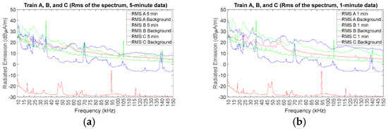
Figure 7.
Measurement results of three different trains in the frequency range of 9 up to 150 kHz: a no-load freight train (Rd2 type without any carriages being pulled) (measurement A: red curve), a loaded freight train (Rc4 type) (measurement B: green curve), and a passenger train (X52 type) (measurement C: blue curve). (a) RMS of the magnetic field spectrum (dBμA/m) for each 200 Hz frequency step for 5 min and background signals; (b) same as (a) but for 1 min and background signals.
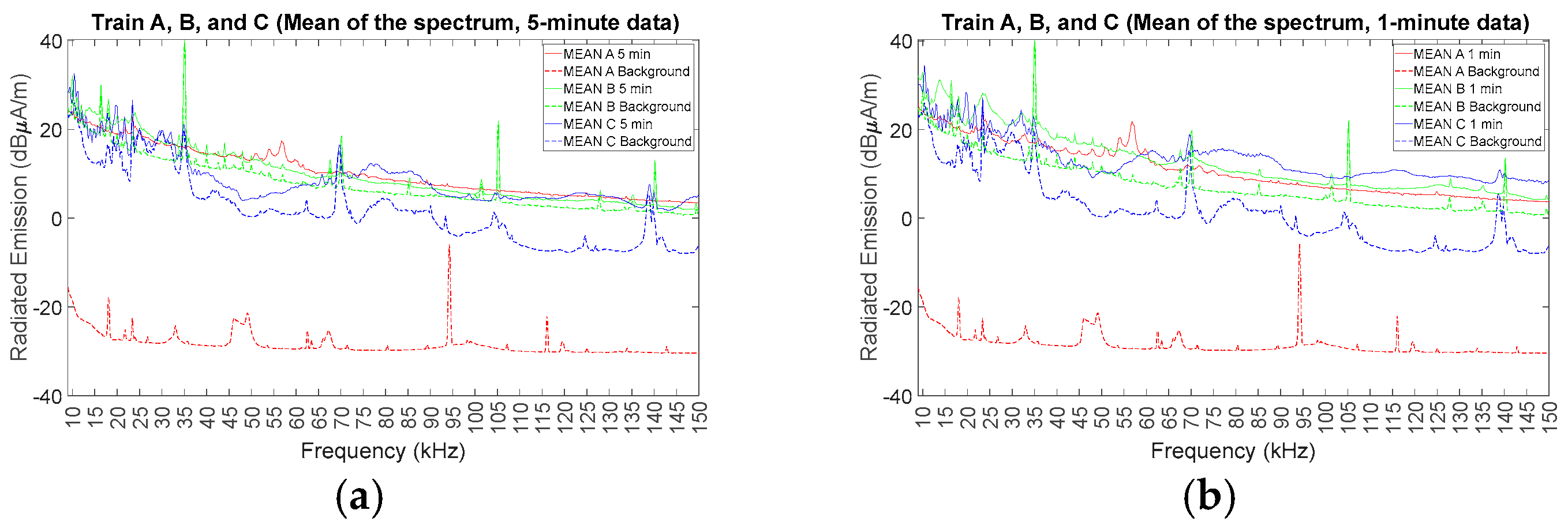
If the mean of the spectrum elements of the 5 min curves be compared for three measurements (Figure 8a), it could be implied that in almost all lower-frequency ranges (below 70 kHz), the loaded freight train (train B) has higher emissions than the passenger train (train C), and for frequency ranges below 50 kHz, the loaded freight train (train B) has higher emissions than the no-load freight train (train A without any carriages being pulled), while for higher-frequency ranges (above 70 kHz), all trains approximately have the same behavior. About the mean of the spectrum elements of 1 min curves (in Figure 8b), almost the same behavior with 5 min curves could be observed.
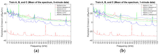
Figure 8.
Measurement results of three different trains in the frequency range of 9 up to 150 kHz: a no-load freight train (Rd2 type without any carriages being pulled) (measurement A: red curve), a loaded freight train (Rc4 type) (measurement B: green curve), and a passenger train (X52 type) (measurement C: blue curve). (a) Mean of the magnetic field spectrum (dBμA/m) for each 200 Hz frequency step for 5 min and background signals; (b) same as (a) but for 1 min and background signals.
4. Discussion and Future Directions
The time-domain antenna output (v) in Figure 3a, Figure 4a and Figure 5a shows different peaks which might be emanating from the difference between type of freight trains and passenger train and also from the fact that the freight train in measurement A was Rd2-type, and it was in the no-load condition (without any carriages being pulled), while the freight train in the measurement B was Rc4 type, and it was in the loaded condition, with around 30 wagons. Even though the freight trains were almost same products from the same company, the passenger train was a product from another company.
The time-domain measurements and time–frequency representation might be a method to solve the repeatability and reproducibility problem. In order to be able to distinguish the logic behind the frequency pattern, (for instance, in order to understand if the reason of the presence of high frequency range could be pantograph arcing, acceleration behavior of the train operator, or something else) it is required to clearly define the operation behavior of the train operator from the four categories (acceleration, cruising, coasting, and braking) before measurements and specify the speed and power at least for the time during which the measurements are recorded (which should be decided to be five minutes or even less or more, in order to have the same framework for different measurements so that fewer uncertainties would result in repeatable and reproducible measurements and outcomes). The time-domain measurements are not covered in the relevant standards. Although the frequency domain measurements have been covered to some extent in the relevant standards, some of the ambiguities have been reported in [22], and it is mentioned that time-domain measurements have their own benefits. In order to have a comprehensive standard, it is needed to define the time of the measurements (as it is mentioned that the start of the measurements in frequency domain shall be from −45 degrees to +45 degrees from antenna location perspective).
It should be noted that the passenger train has higher speed, and it means that for a 5 min time window of data, it might be unfair to compare a passenger train (of type X52 with a maximum speed of around 200 km/h) with a freight train (of type Rc with a maximum speed of 160 km/h or of type Rd with a maximum speed of 135 km/h), and it would be better to judge each train separately from EMC point of view or define a more precise framework which could be applicable for different cases.
In the three measurements reported in this paper, it took around 1 s for train A (a no-load freight train without any carriages being pulled), 25 s for train B (a loaded freight train), and 2 s for train C (a passenger train) to pass the measurement location (considering the whole length of the train).
This should be noted that the catenary of the railway from Bastuträsk to Skelleftehamn (the part of the railway in which the measurements from two freight trains have been taken) is only fed from one of the feeders of a substation located at Bastuträsk. Moreover, one of the other outgoing feeders of this substation also feeds the catenary wire of the railway from Bastuträsk to Kattisträsk (the part of the railway in which the measurements from a passenger train have been taken). As one main switchgear feeds both of the Bastuträsk–Skelleftehamn catenary wire and Bastuträsk–Kattisträsk catenary wire, some voltage variations in the output of the antenna have been observed during the background measurement (although there was no train at least in 60 km distance). This shows the importance of background measurements in de-energized condition of catenary wire (which could be realized through disconnecting the outgoing feeder of main switchgear that is supplying the part of the catenary in which the background measurements are being taken for a short period of time that might be around 5 min or less).
Therefore, the definition of the background for investigating the radiated emissions of the trains is an important point. If a substation with different outgoing feeders that are supplying different sections of the catenary wire be considered, for instance, it could be supposed that train 1 exists in Section 1 of the catenary that is feeding by feeder 1 and train 2 exists in Section 2 of the catenary which is feeding by feeder 2. For instance, if it is intended to record the background of Section 2 (where there is no train on Section 2), it is possible to see the effect of the train 1 which is accelerating in Section 1 (even though there is no train in Section 2, the voltage variations could be observed at the output voltage of the antenna which is located on Section 2 for background measurements); and it could affect the recorded background because both feeders supplying Section 1 and Section 2 are connected to the same switchgear in a substation and has common voltage waveforms. Therefore, it is more precise to measure the pure background when a section is de-energized (for instance, the circuit breaker which is feeding Section 2 should be open so that the changes in other sections could not affect the background measurements in Section 2).
The work presented here is part of an ongoing research work on the study of radiated emissions from railway systems in the frequency range of 9–150 kHz. As a result, future work in this domain may include the following:
- (1)
- Measurements in a controlled environment like a laboratory for simulating different operating modes of the train and environmental conditions like temperature and humidity. This will also facilitate making a comparative assessment between different types of trains.
- (2)
- Measurements in outdoor environments in co-ordination with train operators on the different operating modes of the train.
- (3)
- A comparison of the results of the recorded emissions with other measurements conducted across Europe and in laboratory environments needs to be taken up as part of future work.
- (4)
- Methods like machine learning [48] can be utilized in the future to identify underlying patterns that could not be identified in the present body of work.
- (5)
- Development of prediction models based on tools like artificial intelligence and machine learning [49].
5. Conclusions
The results of three measurements, from a no-load freight train (without any carriages being pulled), a loaded freight train, and a passenger train have been presented in this paper. Some assumptions in the analysis step might lead to different results which could have impacts on the repeatability and reproducibility of the radiated emission measurements from a train. For a specific train with a precoordinated operation mode, the data of radiated emissions could be gathered in time domain with a specific sampling frequency; finally, in the analysis stage, the most important aspects are selection of the time length of analysis period, bandwidth, and the calculation method of the resultant spectrum in frequency domain (RMS, mean, and Max of spectrum at each frequency band). The results of the comparison between radiated emission of three trains revealed the requirement of unique definitions for not only pre- and during-measurement factors but also post-measurement analysis parameters, so that repeatable and reproducible patterns in radiated emission measurement from a train in frequency range of 9 to 150 kHz could be achieved. There are some factors restricting the pattern findings, and clear standard definition of them would enhance the reproducibility of the measurement results: pure background measurement (in energized and de-energized state of the catenary), precoordinated operation mode, speed, and power of the train during the measurement, and the precise definition of the analysis step parameters (the time length of analysis period, the bandwidth, and the calculation method of the resultant spectrum in frequency domain).
Author Contributions
Conceptualization, B.S., P.W. and M.B.; methodology, B.S. and P.W.; software, B.S. and M.G.; writing—original draft preparation, B.S.; writing—review and editing, B.S., P.W., M.G. and M.B.; visualization, B.S. and M.G.; supervision, P.W. and M.B. All authors have read and agreed to the published version of the manuscript.
Funding
This research was funded by the Swedish Transport Administration (Trafikverket).
Data Availability Statement
The data presented in this study are available on request from the corresponding author.
Acknowledgments
We gratefully appreciate the financing and the valuable support of the Swedish Transport Administration (Trafikverket).
Conflicts of Interest
The authors declare no conflicts of interest.
References
- Brenna, M.; Foiadelli, F.; Zaninelli, D. Electrical Railway Transportation Systems; John Wiley & Sons: Hoboken, NJ, USA, 2018. [Google Scholar] [CrossRef]
- Morant, A.; Wisten, Å.; Galar, D.; Kumar, U.; Niska, S. Railway EMI impact on train operation and environment. In Proceedings of the International Symposium on Electromagnetic Compatibility-EMC EUROPE, Rome, Italy, 17–21 September 2012; pp. 1–7. [Google Scholar] [CrossRef]
- Mariscotti, A. Assessment of human exposure (including interference to implantable devices) to low-frequency electromagnetic field in modern microgrids, power systems and electric transports. Energies 2021, 14, 6789. [Google Scholar] [CrossRef]
- Ott, H.W. Electromagnetic Compatibility Engineering; John Wiley & Sons: Hoboken, NJ, USA, 2011. [Google Scholar] [CrossRef]
- Christopoulos, C. Principles and Techniques of Electromagnetic Compatibility; CRC Press: Boca Raton, FL, USA, 2022. [Google Scholar] [CrossRef]
- Markowska, R.; Wróbel, Z. Selected issues of safe operation of the railway traffic control system in the event of exposition to damage caused by lightning discharges. Energies 2021, 14, 5808. [Google Scholar] [CrossRef]
- Wróbel, Z.; Jagiełło, A.S. The Risk of Lightning Losses in a Structure Equipped with RTC Devices According to the Standard EN 62305-2.2008. Energies 2021, 14, 1704. [Google Scholar] [CrossRef]
- Kaleybar, H.J.; Brenna, M.; Foiadelli, F.; Fazel, S.S.; Zaninelli, D. Power quality phenomena in electric railway power supply systems: An exhaustive framework and classification. Energies 2020, 13, 6662. [Google Scholar] [CrossRef]
- Salles, R.S.; Rönnberg, S.K. Review of Waveform Distortion Interactions Assessment in Railway Power Systems. Energies 2023, 16, 5411. [Google Scholar] [CrossRef]
- Salles, R.S.; Rönnberg, S.K.; Mariscotti, A. Waveform Distortion Emission Assessment on Pantograph Measurements from Low-Frequency Railway Electrification. In Proceedings of the 2022 20th International Conference on Harmonics & Quality of Power (ICHQP), Naples, Italy, 29 May–1 June 2022; pp. 1–6. [Google Scholar] [CrossRef]
- Salles, R.S.; Rönnberg, S.K. Interharmonic Analysis for Static Frequency Converter Station Supplying a Swedish Catenary System. In Proceedings of the 2022 20th International Conference on Harmonics & Quality of Power (ICHQP), Naples, Italy, 29 May–1 June 2022; pp. 1–6. [Google Scholar] [CrossRef]
- Salles, R.S.; de Oliveira, R.A.; Rönnberg, S.K.; Mariscotti, A. Analytics of waveform distortion variations in railway pantograph measurements by deep learning. IEEE Trans. Instrum. Meas. 2022, 71, 1–11. [Google Scholar] [CrossRef]
- Mariscotti, A.; Sandrolini, L. Detection of harmonic overvoltage and resonance in AC railways using measured pantograph electrical quantities. Energies 2021, 14, 5645. [Google Scholar] [CrossRef]
- Liu, Q.; Zhang, W.; Cao, G.; Liu, J.; Ye, J.; Wu, M.; Yang, S. Influence of the Catenary Distributed Parameters on the Resonance Frequencies of Electric Railways Based on Quantitative Calculation and Field Tests. Energies 2022, 15, 3752. [Google Scholar] [CrossRef]
- Jin, M.; Yang, Y.; Yang, J.; Wu, M.; Xie, G.; Song, K. Propagation Characteristics and Identification of High-Order Harmonics of a Traction Power Supply System. Energies 2022, 15, 5647. [Google Scholar] [CrossRef]
- Liu, Q.; Sun, B.; Yang, Q.; Wu, M.; He, T. Harmonic Overvoltage Analysis of Electric Railways in a Wide Frequency Range Based on Relative Frequency Relationships of the Vehicle–Grid Coupling System. Energies 2020, 13, 6672. [Google Scholar] [CrossRef]
- Steczek, M.; Chudzik, P.; Szeląg, A. Application of a Non-carrier-Based Modulation for Current Harmonics Spectrum Control during Regenerative Braking of the Electric Vehicle. Energies 2020, 13, 6686. [Google Scholar] [CrossRef]
- Suslov, K.; Kryukov, A.; Ilyushin, P.; Cherepanov, A.; Kryukov, A. Modeling the Effects of Electromagnetic Interference from Multi-Wire Traction Networks on Pipelines. Energies 2023, 16, 4188. [Google Scholar] [CrossRef]
- Jakubowski, K.; Paś, J.; Rosiński, A. The Issue of Operating Security Systems in Terms of the Impact of Electromagnetic Interference Generated Unintentionally. Energies 2021, 14, 8591. [Google Scholar] [CrossRef]
- IEC 62236:2008; Railway Applications—Electromagnetic Compatibility. International Electrotechnical Commission: Geneva, Switzerland, 2008.
- Sadeghi, B.; Westerlund, P.; Salles, R.S.; Wilén, J. Radiated Emissions from an Electric Railway: Review of Methods and Measurements Mainly from 9 KHz to 150 KHz. In Proceedings of the International Conference & Exhibition on Electricity Distribution (CIRED 2023), Rome, Italy, 12–15 June 2023. [Google Scholar] [CrossRef]
- Mariscotti, A. Critical review of EMC standards for the measurement of radiated electromagnetic emissions from transit line and rolling stock. Energies 2021, 14, 759. [Google Scholar] [CrossRef]
- Mariscotti, A. The Electrical Behaviour of Railway Pantograph Arcs. Energies 2023, 16, 1465. [Google Scholar] [CrossRef]
- Jin, M.; Hu, M.; Li, H.; Yang, Y.; Liu, W.; Fang, Q.; Liu, S. Experimental Study on the Transient Disturbance Characteristics and Influence Factors of Pantograph–Catenary Discharge. Energies 2022, 15, 5959. [Google Scholar] [CrossRef]
- Li, X.; Zhu, F.; Lu, H.; Qiu, R.; Tang, Y. Longitudinal propagation characteristic of pantograph arcing electromagnetic emission with high-speed train passing the articulated neutral section. IEEE Trans. Electromagn. Compat. 2018, 61, 319–326. [Google Scholar] [CrossRef]
- Persichini, R.D.; Di Febo, D.; Calà, V.; Malta, C.; Orlandi, A. EMC analysis of axle counters in the Italian railway network. IEEE Trans. Electromagn. Compat. 2014, 57, 44–51. [Google Scholar] [CrossRef]
- Interfaces between Control-Command and Signalling Trackside and Other Subsystems (ERA ERTMS/ETCS UNIT, European Railway Agency, ERTMS Unit, ERA_ERTMS_033281 v40.doc, 20/09/2018). Available online: https://www.era.europa.eu/system/files/2022-11/Interface%20between%20control-command%20signalling%20trackside%20and%20other%20subsystems%20%28v.3%2004-12-2015%29.pdf.pdf (accessed on 29 September 2024).
- Angrisani, L.; D’Arco, M.; De Benedetto, E.; Duraccio, L.; Lo Regio, F. Broadband Power Line Communication in Railway Traction Lines: A Survey. Energies 2023, 16, 6387. [Google Scholar] [CrossRef]
- Yudhistira Yudhistira, Y.Y.; Trivida, E.; Wijanarko, T.A.W.; Nugroho, H.W.; Mandaris, D. Electromagnetic interference measurement for axle counters light rapid transit railway in Indonesia. Int. J. Electr. Comput. Eng. 2022, 12, 4632–4639. [Google Scholar] [CrossRef]
- Paś, J.; Rosiński, A.; Wetoszka, P.; Białek, K.; Klimczak, T.; Siergiejczyk, M. Assessment of the Impact of Emitted Radiated Interference Generated by a Selected Rail Traction Unit on the Operating Process of Trackside Video Monitoring Systems. Electronics 2022, 11, 2554. [Google Scholar] [CrossRef]
- Nagórny, B.; Maćkowiak, A.; Rokossowski, M.; Sieczkarek, K.; Szczepański, R.; Warzyński, T. Implementation of the test method for trackside emissions of magnetic disturbances from rolling stock according to ERA/ERTMS/033281. Rail Veh./Pojazdy Szyn. 2022, 1–2, 62–67. [Google Scholar] [CrossRef]
- Brillante, S.; Hill, R.J.; Pozzobon, A.; Pozzobon, P.; Sciutto, G. Modelling for electromagnetic interference assessment in electric railway traction systems. In Proceedings of the International Conference on Electric Railways in a United Europe, Amsterdam, The Netherlands, 27–30 March 1995. [Google Scholar] [CrossRef]
- Pranay, S.; Prerna, S.; Singh, L.P.; Deswal, S.S. Mitigation of Electromagnetic Interference in Rolling stock. Int. J. Electr. Electron. Comput. Eng. 2013, 2, 22–27. [Google Scholar]
- Shi, L.; Liang, J.; Liu, Y.; Zhao, Y.; Li, X. Electromagnetic Environment Assessment and Safety Research of Electrified High-Speed Railway Carriages. Electronics 2024, 13, 740. [Google Scholar] [CrossRef]
- Mantiply, E.D.; Pohl, K.R.; Poppell, S.W.; Murphy, J.A. Summary of measured radiofrequency electric and magnetic fields (10 kHz to 30 GHz) in the general and work environment. Bioelectromagn. J. Bioelectromagn. Soc. Soc. Phys. Regul. Biol. Med. Eur. Bioelectromagn. Assoc. 1997, 18, 563–577. [Google Scholar] [CrossRef]
- Giri, M.; Sadeghi, B.; Rönnberg, S.; Johansson, J.; Ekman, J. Observations of radiated and conducted emissions from an Electric Plane charging station. In Proceedings of the 2023 International Symposium on Electromagnetic Compatibility–EMC Europe, Kraków, Poland, 4–8 September 2023; pp. 1–6. [Google Scholar] [CrossRef]
- Bollen, M.H.; Gu, I.Y. Signal Processing of Power Quality Disturbances; John Wiley & Sons: Hoboken, NJ, USA, 2006. [Google Scholar] [CrossRef]
- Gu, Y.H.; Bollen, M.H. Time-frequency and time-scale domain analysis of voltage disturbances. IEEE Trans. Power Deliv. 2000, 15, 1279–1284. [Google Scholar] [CrossRef]
- Larsson, E.O.A.; Lundmark, C.M.; Bollen, M.H.J. Measurement of current taken by fluorescent lights in the frequency range 2–150 kHz. In Proceedings of the 2006 IEEE Power Engineering Society General Meeting, Montreal, QC, Canada, 18–22 June 2006. [Google Scholar] [CrossRef]
- Gu, I.Y.H.; Bollen, M.H. Estimating interharmonics by using sliding-window ESPRIT. IEEE Trans. Power Deliv. 2007, 23, 13–23. [Google Scholar] [CrossRef]
- Ronnberg, S.K.; Wahlberg, M.; Bollen, M.H.J.; Lundmark, C.M. Equipment currents in the frequency range 9–95 kHz, measured in a realistic environment. In Proceedings of the 2008 13th International Conference on Harmonics and Quality of Power, Wollongong, Australia, 28 September–1 October 2008; pp. 1–8. [Google Scholar] [CrossRef]
- Larsson, E.A.; Bollen, M.H.; Wahlberg, M.G.; Lundmark, C.M.; Rönnberg, S.K. Measurements of high-frequency (2–150 kHz) distortion in low-voltage networks. IEEE Trans. Power Deliv. 2010, 25, 1749–1757. [Google Scholar] [CrossRef]
- Sakar, S.; Rönnberg, S.K.; Bollen, M. Interharmonic emission in AC–DC converters exposed to nonsynchronized high-frequency voltage above 2 kHz. IEEE Trans. Power Electron. 2020, 36, 7705–7715. [Google Scholar] [CrossRef]
- Busatto, T.; Rönnberg, S.K.; Bollen, M.H. Comparison of models of single-phase diode bridge rectifiers for their use in harmonic studies with many devices. Energies 2021, 15, 66. [Google Scholar] [CrossRef]
- Shimi, S.L.; Delgado, A.E.; Rönnberg, S.K.; Bollen, M.H. Evaluation of Medium Voltage Network for Propagation of Supraharmonics Resonance. Energies 2021, 14, 1093. [Google Scholar] [CrossRef]
- Sierra-Fernández, J.M.; Rönnberg, S.; Gonzalez de la Rosa, J.J.; HJ Bollen, M.; Palomares-Salas, J.C. Application of spectral kurtosis to characterize amplitude variability in power systems’ harmonics. Energies 2019, 12, 194. [Google Scholar] [CrossRef]
- Abid, F.; Busatto, T.; Rönnberg, S.K.; Bollen, M.H. Intermodulation due to interaction of photovoltaic inverter and electric vehicle at supraharmonic range. In Proceedings of the 2016 17th International Conference on Harmonics and Quality of Power (ICHQP), Belo Horizonte, Brazil, 16–19 October 2016; pp. 685–690. [Google Scholar] [CrossRef]
- de Oliveira, R.A.; Nakhodchi, N.; De Souza Salles, R.; Rönnberg, S.K. Deep Learning Graphical Tool Inspired by Correlation Matrix for Reporting Long-Term Power Quality Data at Multiple Locations of an MV/LV Distribution Grid. In Proceedings of the 27th International Conference on Electricity Distribution (CIRED 2023), Rome, Italy, 12–15 June 2023. [Google Scholar]
- Peng, T.; Gan, M.; Ou, Q.; Yang, X.; Wei, L.; Ler, H.R.; Yu, H. Railway cold chain freight demand forecasting with graph neural networks: A novel GraphARMA-GRU model. Expert Syst. Appl. 2024, 255 Pt B, 124693. [Google Scholar] [CrossRef]
Disclaimer/Publisher’s Note: The statements, opinions and data contained in all publications are solely those of the individual author(s) and contributor(s) and not of MDPI and/or the editor(s). MDPI and/or the editor(s) disclaim responsibility for any injury to people or property resulting from any ideas, methods, instructions or products referred to in the content. |
© 2024 by the authors. Licensee MDPI, Basel, Switzerland. This article is an open access article distributed under the terms and conditions of the Creative Commons Attribution (CC BY) license (https://creativecommons.org/licenses/by/4.0/).