Comparison of Optimal SASS (Sparsity-Assisted Signal Smoothing) and Linear Time-Invariant Filtering Techniques Dedicated to 200 MW Generating Unit Signal Denoising

Abstract

Performing reliable calculations of power system dynamics requires accurate models of generating units. To be able to determine the parameters of the models with the required precision, a well-defined testing procedure is used to record various unit transient signals. Unfortunately, the recorded signals usually contain discontinuities, which complicates the removal of the existing harmonic interferences and noise. A set of four transient signals recorded during typical disturbance tests of a 200 MW power-generating unit was used as both training and research material for the signal denoising/interference removal methods compared in the paper. A systematic analysis of the measured transient signals was conducted, leading to the creation of a coherent mathematical model of the signals. Next, a method for denoising power-generating unit transient signals is proposed. The method is based on Sparsity-Assisted Signal Smoothing (SASS) combined with optimization algorithms (simulated annealing and Nelder-Mead simplex) and is called an optimal SASS method. The proposed optimal SASS method is compared to its direct Linear Time-Invariant (LTI) competitors, such as low-pass and notch filters. The LTI methods are based on the same filter types (Butterworth filters) and zero-phase filtering principle as the SASS method. A set of specially generated test signals (based on a developed mathematical model of the signals) is used for the performance evaluation of all presented filtering methods. Finally, it is concluded that—for the considered class of signals—the optimal SASS method might be a valuable noise removal technique.

1. Introduction

Modern power systems are marked by their complex and dynamic characteristics. They are undergoing significant changes, largely due to the widespread integration of distributed generation units that utilize renewable energy sources [1]. As a result, there is a growing need for improved strategies in the control and management of these advanced systems [2,3]. This transformation greatly impacts areas such as communication, measurement, and the modeling of power systems and their components [4,5,6,7].

When introducing a new device into the power system—whether it be a generating unit, transmission or conversion system, controller, or any other equipment—it is essential to analyze the device’s model under both normal and abnormal conditions across short- and long-term operational scenarios [8,9]. However, conducting such testing and analysis on a live power system is impractical due to various safety and economic concerns [2]. This is especially true in relation to electromagnetic transients and dynamic stability, where the design and reliable operation of today’s power systems encounter significant challenges [10]. Incorrect decisions or inaccurate forecasts can have disastrous consequences, potentially resulting in instability, isolated operation, or even a blackout [11,12]. As a result, scientists and engineers must rely extensively on computer simulations to comprehend the operation and control of power systems [13,14,15,16].

A key factor in utilizing computer simulations effectively is the accuracy of the input data [6,17]. Alongside the algorithms and models, precise measurement data are essential for producing correct and reliable simulation outcomes. It is widely agreed within the industry that creating accurate models of generating units and their control systems is crucial for defining operational security limits, as well as for simulating and understanding system behavior during disturbances [15,18].

The authors have frequently faced challenges when performing calculations for an excitation system operating with a high-power generator [6,19,20,21,22]. Each time, one of the crucial problems was to obtain the most reliable measurement data: the transient waveforms recorded under the application of appropriate disturbance tests [6,19,23,24]. These waveforms served as the basis for calculations and were also used as reference and verification data to ensure the reliability and accuracy of the calculations. Despite using professional measuring equipment, such as specialized commercial recorders (e.g., Fluke (Fluke, Eindhoven, The Netherlands), Sonel (Sonel S.A., Świdnica, Poland), A-eberle (A. Eberle GmbH & Co., Nürnberg, Germany)) and custom-built recorders for specific test standards such as Energotest (Spie Energotest Sp. z.o.o., Warszawa, Poland) or Kared (Kared Sp. z.o.o., Kowale, Poland) [25], the operating environment of a large power-generating unit is a measurement challenge [20]. The recorded signals are influenced by noise, interferences, and unintended interactions and couplings, all of which combine and interfere with the test signals.

Selecting and fine-tuning the appropriate filtering or approximation methods for the measured waveforms is a time-consuming process and often fails to produce consistent results. Still, it must be performed for each test conducted despite being a secondary element of the research. Therefore, the authors have decided to conduct a systematic analysis of the measured transient signals, which results in a coherent mathematical model [22]. When the model is ready, a literature review may be carried out, and a potentially optimal method for analyzing transient signal filtering/approximation might be chosen [22]. Next, the chosen method is combined with advanced optimization algorithms to find its optimal version, which allows for finding the best parameter values [22]. Finally, the proposed optimal method is compared with some well-known reference filtering techniques.

2. Overview of 200 MW Generating Unit and Measured Transient Signals

Figure 1 presents a schematic of the generator-excitation system for a 200 MW class generating unit. This AC-type excitation system is specifically designed to meet the DC field requirements of a high-power 235 MW synchronous generator powered by a steam turbine. The design generally consists of three key sub-systems: a voltage regulator, an exciter, and a diode rectifier.

The regulator processes and amplifies input control signals to a level and form that is suitable for the exciter. An AC exciter is installed on the same shaft as the turbine generator, and its terminals are connected to a stationary rectifier; this setup provides DC power to the generator field winding. The limiters present at every stage of signal processing ensure that the capability limits of the exciter and generator are not exceeded. All of the aforementioned components are nonlinear, and therefore, their modeling is a challenging task [26].

The model concept is based on a modified AC-type model, as outlined in IEEE 421.5 Standard [8]. This research employs an original electromachine excitation system model, which includes components such as a voltage regulator, an auxiliary regulator, an exciter, and an excitation voltage formation system. A detailed and comprehensive description of this model is available in [6,20]. The model’s classification is somewhat flexible, as its actual configuration depends on the availability of measurement signals.

The schematic diagram of the generating set (Figure 1) outlines the following measurable signals: reference voltage (U_ref), generator terminal voltage (U_g), regulator output voltage (U_r), exciter field current (I_fe), generator field current (I_fd), and generator field voltage (E_fd). These signals can be recorded and subsequently used in various scientific analyses, particularly for examining transient states within the power system. Additionally, the issue of parameter estimation is important. It has been observed that significant discrepancies often exist between parameters provided by manufacturers and those obtained through direct measurement [6,15].

In order to ensure that generating units can operate reliably and safely in different operating conditions, it is important to subject them to various disturbances during testing. The specific tests will depend on the type of generating unit and the industry standards as well as the regulations that apply to it.

IEEE standards offer valuable guidance and recommendations for testing and evaluating the performance of all power unit components, including turbines and their governors, power generators, and excitation systems with their voltage controls. IEEE Standard 421.2 [17] provides specific guidelines for the excitation systems of synchronous generators. The standard provides detailed recommendations for the test procedures, equipment, and instrumentation requirements. It also provides recommendations for interpreting the test results and identifying any performance issues that may need to be addressed. It recommends the voltage step change test as the testing procedure.

3. Disturbance Test and Analysis of the Measured Signals

The voltage step change test is a widely used method for assessing the performance of closed-loop excitation control systems [17,26]. This transient response test involves a step change in the reference voltage of the voltage regulator and monitoring the excitation system’s response. The test aims to evaluate the system’s performance under sudden load changes or other disturbances and is also used to identify and validate the parameters of the excitation system model [27].

The standard recommends that the voltage step change should be performed with a step size not greater than 20% of the rated voltage and that the excitation system should be able to maintain stable voltage regulation within a specified range of voltage deviation [28].

The waveforms used in this research were recorded at the power plant during routine tests conducted for the recommissioning of the large power generator (TWW-200-2A, manufacturer Dolmel (Wrocław, Poland); modified by EthosEnergy Poland S.A. 200@235 MW (Lubliniec, Poland)). A 12-bit resolution and 32 kHz sampling rate were used during a synchronous recording of all of the signals. Since the 32 kHz sampling rate is far too high, all signals were filtered by an anti-aliasing filter and downsampled to 4 kHz. This sampling rate is consistent with the considered mathematical model of the excitation system and has been sufficient to capture all relevant signal parameters. Most importantly, this sampling rate is enough to preserve the edges/slopes of the signal without reducing their steepness.

Figure 2 shows a brief summary of the recorded waveform of the generating unit during a step change in the regulator’s reference voltage [22]. As can be seen, the waveforms change shape in the successive processing stages. Some disturbances disappear or lose their strength, and others appear in their place.

In Figure 3, the amplitude Fourier spectrum of the recorded signals is presented. The amplitude spectrum reveals some characteristic interferences, which are discussed further for each individual signal.

In the presented set of signals, one sinusoidal signal (U_g) stands out, the use of which requires the extraction of its envelope (in Figure 2, just the U_g’s envelope is shown). This problem is a separate issue and is out of the scope of this paper.

The reference voltage signal reflects the step change in a given quantity (Heaviside unit step). Its bump level relates to the expected change in the value of the generator armature voltage (after regulation).

The regulator output voltage U_r is a signal produced in a digitally controlled automatic voltage regulator (AVR) [29]. Mostly, the conventional PID regulator is used to enhance the dynamic performance and stability of AVR due to its robustness, simple design, and easy implementation [30,31]. During modeling, finer control action is offered by FOPID, which ensures superior performance and tuning flexibility [21,32]. The signal value can only assume positive values and changes in the range from 0 to 10 V. It is also an input signal in the regulator’s executive circuit (the so-called additional regulator). U_r signal in the time domain (Figure 2) contains two sharp steps (jump discontinuities at t = 0.8 s and t = 4.3 s), which are the result of the test disturbances. In between the steps, the waveform changes smoothly and rather slowly (which comes from the voltage regulator time constants) except the point t = 1.1 s, where a sharp corner appears (removable discontinuity), which comes from a lower bound of the U_g value. In other words, the signal can be approximated by smooth (differentiable) functions except for the discontinuity points. Considering the amplitude spectrum of the U_r (Figure 3), it is observably free of harmonic interferences but with a visible amount of noise (especially in the higher frequency range).

The signal of exciter field current Ife emerged as a product of the cooperation of the excitation transformer, high frequency (HF) rotating machine, and the power electronics device. U_r signal, which was previously worked out in a voltage regulator, is amplified in an additional regulator built on the basis of an IGBT transistor and a pulse width modulation system (PWM). The amplified signal is routed to the rotor winding of the AC exciter. The power electronic components are fed from the three-phase unit auxiliary transformer installed in close proximity. The high-frequency (HF) exciter is installed on a common shaft with a power generator and turbine, and it operates with a rated frequency of 500 Hz. The special feature of current I_fe is also entails the impossibility of assuming negative values [20]. In the I_fe time domain waveform (Figure 2), the level of interferences is considerably higher than in the case of U_r. The first step at 0.8 s is less sharp and should, thus, be regarded as two separate removable discontinuities at the beginning and end of the slope. The second step at 4.3 s is even smoother, and it also should be regarded as two separate removable discontinuities connected by a continuous function. The edge at 1.2 s is probably round enough not to be treated as a discontinuity point any longer. Looking at the amplitude spectrum of I_fe (Figure 3), it can be observed that apart from the noise, harmonic components are also visible, with two of them located at 500 Hz and 1 kHz. These components are the base frequency and second harmonic of exciter field current and have amplitudes about 22 dB and 25 dB higher than the nearby noise floor level.

The AC signal obtained in the output of the exciter is rectified in a stationary six-pulse diode rectifier [8]. With respect to the current value of the generator field current (I_fd), the voltage-forming system produces the generator field voltage (E_fd). The E_fd waveform (Figure 2) is generally a clean signal with a low level of interference. However, there is still some visible noise and two harmonic components located at 50 Hz (component related to the power grid main frequency) and 1 kHz (from the excitation system), which is observable in the amplitude spectrum (Figure 3). The 50 Hz component has an amplitude about 18 dB higher than the noise floor, and the 1 kHz component is about 23 dB higher than the noise floor. From a time domain perspective, at a macro scale, there are five removable discontinuities at 0.8, 0.9, 1.4, 4.3, and 4.5 s (the last one is probably smooth enough not to be regarded as discontinuity any longer).

I_fd should be recognized as a result of applying the E_fd signal to the rotor winding of the generator. The application is executed through slip rings. The massive inductance and the influence of the armature circuit of the generator have the greatest impact on the parameters of this signal [19]. The I_fd waveform is generally even smoother than the I_fe (Figure 2). The removable discontinuities can be observed at 0.8, 1.4, and 4.3 s. The total interference level seems to be even higher than for the I_fe, and its main source is the noise and harmonic component at f = 1 kHz (with an amplitude about 20 dB higher than the noise floor), which is observable in the amplitude spectrum of the signal (Figure 3)

4. Mathematical Model of the Measured Signals

As shown in Section 3, the presented signals are a combination of smooth differentiable functions with two kinds of discontinuity points (jump and removable) with noise and some harmonic interferences. Moreover, the slopes of the functions might be very different at different points of the signals. The generalized model of the signals is a sum of the output signal in a certain measurement point and some interferences, which are as follows [22]:

• The base frequency of the power system, which is equal to 50 Hz (only the generator field voltage E_fd contains this component).
• Harmonic components from various sources. These interferences can be observed in generator field voltage E_fd (1000 Hz), the exciter field current I_fe (500 Hz and 1000 Hz), and the field current I_fd.
• Wideband noise, which is present in all signals.

Taking into consideration all of the mentioned interferences, the mathematical model of the signal can be written as follows [22]:

$$s^P\left(t\right)=s\left(t\right)+h\left(t\right)+n\left(t\right)$$

(1)

where

• s^P(t)—the measured signal (with noise and interferences);
• s(t)—signal free of any interferences (the clean signal);
• h(t)—harmonic interferences, which can be described as $\sum _{i=1}^n{A}_i\sin \left(2\pi f_{i}t\right)$, where i is the harmonic number;
• n(t)—wideband noise.

Since the presented methodology is the same for all measured signals, the proposed filtering/approximation methods should be flexible enough to successfully adapt to different kinds and ranges of interferences. Since some of the signals contain removable discontinuities (e.g., I_fe, E_fd, I_fd) and/or jump discontinuities (e.g., U_r), it is hard to find a simple LTI filter (e.g., a low-pass filter) which removes all the interferences and does not distort the clean signal s(t).

The authors believe that the presented model might be a valuable reference point for other similar devices in similar measurement scenarios. The presented model is very general and can represent any signal which contains noise and harmonic interferences. In the case of different kinds of interferences (inharmonic), the model should be changed or extended.

5. Review of Existing Filtering/Approximation Methods and General Assumptions

There are many existing methods which can be used to remove the interferences from the signal described by Equation (1). Most of these methods belong to one of the following categories [22]:

• The first category is the methods, which try to filter out the interferences and noise (h(t) and n(t) in (1)). The number of methods which can be named here is very broad. Some of the most popular ones are those based on typical LTI digital filters (e.g., low-pass, stop-band, and notch filters), some commonly used nonlinear filters (e.g., the median filter), or some manner of adaptive filter (like the Wiener filter) [33]. The demand for computing power in the case of these methods is relatively small, and the design algorithms are relatively simple. There are also much more complex methods which require much more computing power, like those based on neural networks [34], deep learning [35], or Sparsity-Assisted Signal Smoothing (SASS) [36]. The choice of certain methods depends on many factors, but one of the most important is the character of the interferences in comparison with the clean signal. In situations where it is difficult to separate the interferences from the clean signal (e.g., if they occupy the same bandwidth), the standard LTI approach might not be sufficient enough. It is also well known that filters can introduce additional artifacts (like ringing and overshooting in the time domain). These artifacts can change the shape of the signal significantly, which is usually unacceptable in dynamical systems modeling.
• The second category is the methods which try to approximate the clean signal s(t) from the measured signal s′(t). It can be a simple Savitzky-Golay polynomial approximation [37], a more advanced method using some manner of signal transform (for example, wavelet transform [38]), or a model-based Bayesian filter (like the extended Kalman filter [39]). In this approach, the most difficult part is to find the approximating function that is a good fit for the shape of the s(t) signal. This can be a challenging task, especially if the signals contain discontinuities and steep slopes. This group of methods can also introduce some artifacts to the signal (for example, the wavelet denoising is well known for its pseudo-Gibbs effect [40]). It is worth writing here that the approximation methods are very often implemented in the form of FIR (Finite Impulse Response) or IIR (Infinite Impulse Response) digital filters in practical implementations. The Savitzky-Golay method is implemented as FIR filters [41], and the discrete wavelet transform is usually implemented using the quadrature mirror filters (QMF) [42].

Since there are hundreds of existing filtering techniques, it is impossible to name all of them here. For someone who would like to further explore the topic, papers [39,40] might be good reference points.

The authors of these papers, based on previous experience and a broad literature review, have chosen a selection of methods which will be further investigated in this paper. This choice has been made with the following assumptions in mind:

• The time alignment of the clean signal should not be changed.
• Steep transition slopes and discontinuities of jump and removable kind should be preserved.

In other words, an ideal method should not introduce any delay to the signal and should not change the shape of the clean signal.

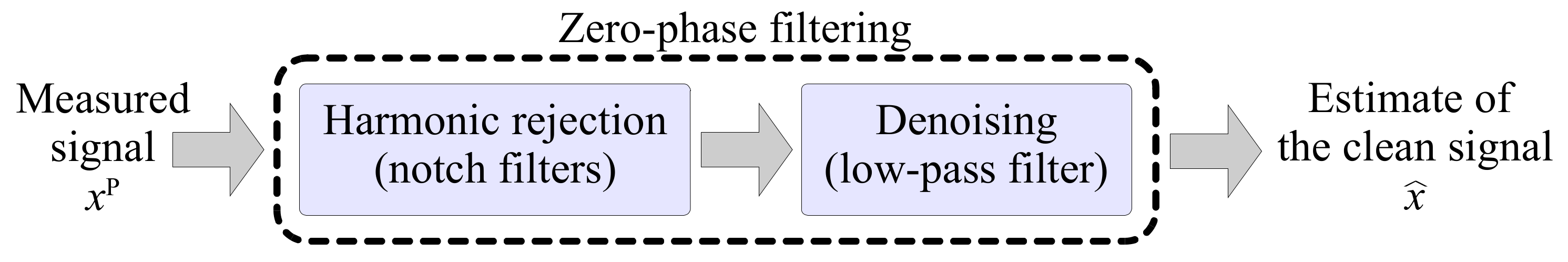
6. Sparsity-Assisted Signal Smoothing (SASS) and Reference LTI Filtering Methods

The SASS method has been chosen as a potential leader in power generator signal denoising [22,36]. The method was designed to remove the noise from a signal with discontinuities. SASS uses low-pass filtering and total variation denoising (TVD). The algorithm is based on banded Toeplitz matrices and zero-phase recursive discrete-time filtering of finite-length data. Details of the method are described in [36], and the overview of the method can also be found in [22]. However, to give a general overview of the method and for convenience, a brief introduction of the method is presented here.

First, a discrete time domain clean signal x[n] is modeled as a sum of two components: the high-frequency component x₁[n] and low-frequency component x₂[n]:

$$x\left[n\right]=x_1\left[n\right]+x_2\left[n\right]x\left[n\right],x_1\left[n\right],x_2\left[n\right]\in R,$$

(2)

There is a general assumption about the x₁[n] component that the D(x₁[n]) is sparse, where D(.) is a matrix representing K-order discrete-time difference. In further equations, the sample number n is omitted for a shorter notation (the same as in [36]). For the low-frequency signal x₂, it is assumed that a zero-phase low-pass filter H can be found, which does not alter the x₂ signal but removes the noise:

$$x_2=H\left(x_2\right), x_{2 }\approx H\left(x_2+w\right),$$

(3)

where w is an additive white Gaussian noise (AWGN). The H filter is used to remove the noise from the low-pass signal x₂. This is achieved by removing the high-frequency components (most of the noise w) from the signal. This can be achieved without significant changes in the signal’s shape because all the high-frequency details (steep slopes, discontinuity points, etc.) are preserved in x₁, and this signal is not low-pass filtered.

The model of the noisy signal (the measured signal) x^P is defined as a sum of the x signal (the clean signal) and the AWGN w:

$$x^P=x+w,$$

(4)

$$x^P=x_1+x_2+w.$$

(5)

The x^P signal is assumed to be a sum of differentiable high-frequency component x₁ with a sparse derivative, the low-frequency signal x₂, and a Gaussian white noise w.

The idea of the method is to find the estimate of an unknown clean signal x using the noisy measurement data x^P. In the first step, Equation (5) can be rearranged into the following:

$$x^P-x_1=x_2+w.$$

(6)

Considering the (3), the following can be written:

$$x_2\approx H(x_2+w)\Rightarrow x_2\approx H(x^P-x_1).$$

(7)

Interpreting (7), it can be said that if the x₁ is known, then the x₂ can be obtained by low-pass filtering $x^P$ − x₁. In this case, the estimate ${\widehat{x}}_2$ can be expressed as follows:

$${\widehat{x}}_2\approx H(x^P-{\widehat{x}}_1).$$

(8)

The clean signal estimate can be written as a sum of the estimates of the low- and high-frequency components:

$$\widehat{x}={\widehat{x}}_1+{\widehat{x}}_2.$$

(9)

Then, using (8), the following can be written:

$$\widehat{x}={\widehat{x}}_1+H(x^P-{\widehat{x}}_1),$$

(10)

$$\widehat{x}={(I-H)(\widehat{x}}_1)+H(x^P),$$

(11)

$$\widehat{x}={G(\widehat{x}}_1)+H(x^P),$$

(12)

where G = I − H is a zero-phase high-pass filter (more about H and G filters can be found in [36]). Here, another assumption is made that the high-pass filter G admits the factorization G = RD (.). In this factorization, the D (.) is a matrix representing K-order discrete-time difference, R is a corresponding Toeplitz matrix (details about the factorization can be found in Section 2.3 of [36]), and G could be a Butterworth filter. Considering these assumptions, the following can be written:

$$\widehat{x}={R\left(D\right(\widehat{x}}_1\left)\right)+H\left(x^P\right),$$

(13)

$$\widehat{x}=R\left(\widehat{u}\right)+H\left(x^P\right),$$

(14)

where $\widehat{u}:=D\left({\widehat{x}}_1\right)$ is sparse. To estimate $\widehat{u}$, a sparse-regularized least-squares optimization problem can be formulated:

$$\widehat{u}=arg \underset{u}{\min }\{{\displaystyle \frac{1}{2}}{‖x^P-R\left(u\right)+H\left(x^P\right)‖}_2^2+\lambda {‖u‖}_1\},$$

(15)

where

• ${‖x‖}_2^2:=\sum _n{x}^2\left[n\right]$, ${‖x‖}_1:=\sum _n\left|x\left[n\right]\right|$, and regularization parameter λ > 0.

This problem can be solved using one of the available methods, like forward-backward splitting (FBS) [36].

Theoretically, the SASS method should serve as an ideal solution for the transient signals from the power generator, given that these signals contain smooth (low-frequency) segments interspersed with local discontinuities and steep slopes. The low-pass filtering characteristic of SASS is expected to eliminate the noise component (n(t) in (1)) present in the smooth areas of the signal. Conversely, the steep slopes or sharp corners near the discontinuities should be preserved in the output signals. Additionally, since SASS employs zero-phase filtering, it ensures the time alignment between the input and output signals automatically, and when using a first-order Butterworth filter, there are no ringing or overshooting effects in the time domain (higher-order filters can also be utilized). However, the method was not intended to eliminate anything beyond noise from the signal, which means that the harmonic components (h(t) in (1)) present in the input signals may pose a significant challenge to the approach. The primary issue lies in identifying the optimal set of parameters for a specific input signal, a matter that will be elaborated upon in the following sections. An example of SASS denoising is illustrated in Figure 4, where it can be observed that noise was effectively removed without compromising the steep slopes in the signal, as depicted by the sparse derivative estimate. Moreover, there are no noticeable parasitic oscillations in the flat portions of the signal, which are commonly associated with polynomial interpolation artifacts (Runge’s phenomenon).

The SASS method will be compared with a reference LTI noise and harmonic rejection method based on a low-pass filter for denoising and notch filters for harmonic rejection. These filters are one of the typical first-choice methods in the case of denoising (low-pass filters) and harmonic rejection (notch filters) [20,24,36]. A block diagram of this method is presented in Figure 4.

The notch filters (Figure 4) are second-order filters [43], and a low-pass digital filter is a Butterworth filter [44]. Filters were designed using Matlab’s R2020a “iirnotch” and “butter” methods, respectively. It is also important to mention that each filter was applied to the signal using zero-phase filtering (Matlab’s “filtfilt” method), which has the following consequences:

• Zero phase distortion.
• A filter transfer function equal to the squared magnitude of the original filter transfer function.
• An effective filter order that is double the order of the given filter.
• Because the zero-phase filtering is implemented by reversing the input signal samples order, this method cannot be used in real-time applications (the whole signal must be known before the filtering is started). This makes the presented methods suitable for off-line analysis only.

The Butterworth low-pass filter and zero-phase filtering were used to keep the reference method as close as possible to the SASS method in terms of the filter type and filtering method. This approach allows showing how the SASS method (which is internally also based on Butterworth filters and zero-phase filtering) compares to its direct competitors. In the authors’ opinion, this sets a well-defined and a fair reference point for direct comparison between the considered methods.

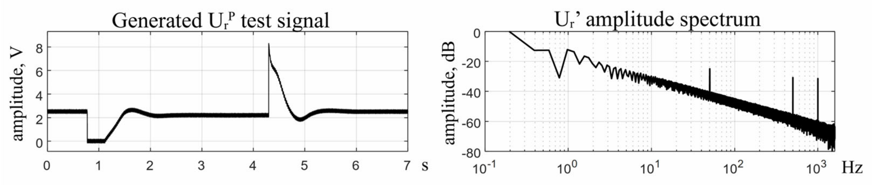
7. Test Signal Synthesis

To facilitate quantitative comparative analysis of the signal denoising results across all examined methods, it is essential to utilize test signals with known parameters. The test signals for the optimization procedure were developed using the following steps [22]:

• Initially, reference (clean) signals were generated from a model of the power-generating unit operating under the same disturbance test conditions as the actual generator during the measurements. These clean signals correspond to the s(t) component in Equation (1) and serve as a baseline for assessing the filtering/approximation quality of all tested methods.
• In the subsequent step, white Gaussian noise was introduced to the clean signals, corresponding to the n(t) component in Equation (1). The signal-to-noise ratio (SNR) was adjusted to closely match that of the measured signals. To maintain the amplitude spectrum profile of the noise consistent with the measurements, it was generated at a sampling rate of 32 kHz and then downsampled to 4 kHz using the same antialiasing filter applied to the measured signals.
• In the last step, three harmonic components (represented by h(t) in Equation (1)) were added to the signals. The frequencies of the components are 50, 500, and 1 kHz, and the amplitudes (measured above the noise floor) are approximately 18 dB, 22 dB, and 25 dB, respectively. These harmonic components were introduced under a worst-case scenario, where their amplitudes matched the maximum amplitudes observed in all of the measured signals. An example of the Ur’ signal, including noise and harmonic components, is illustrated in Figure 5.

The distorted signals are used as input signals for all tested filtering/approximation methods. Exactly the same test signals were used in [22] to make the results directly comparable with those presented in his paper.

8. Optimization Problem Definition and the Proposed Optimal SASS Method

In general, the same methodology was used to optimize the parameters of all of the considered methods (including the method presented in [22]). This approach ensures a fair comparison of all considered methods. An overview of the optimization procedure is shown in Figure 6.

The input data for the optimization process includes the model-generated reference/clean signals, the test signals that have been subjected to added noise and harmonic interference (with further details about these signals provided in Section 7), and the initial parameter values for the optimization procedure. The effectiveness of each filtering method is evaluated by comparing the filtered noisy signals to their corresponding reference signals (as outlined in Equations (18) and (19)), which will be discussed in detail later in this section.

The specifics of the optimization process are highly dependent on the filtering method employed (see

Table 1. Optimization algorithms used for different filtering methods [22].

Filtering Method	Optimization Algorithm	Optimized Parameters
Butterworth low-pass filter	Gradient	Filter cut-off frequency
3 notch filters	Simulated annealing + gradient	Filters width
3, 2, or 1 notch filter + low-pass Butterworth	Simulated annealing + gradient	Notch filter width, low-pass filter cut-off frequency
Optimal SASS	Simulated annealing + Nelder-Mead simplex	Low-pass cut-off frequency, regularization parameter

). For the simple low-pass filtering, a gradient algorithm proved sufficient to determine the optimal cut-off frequency of the filter. For notch filters and combinations of notch and low-pass filters, a bounded simulated annealing approach was initially applied to identify the region of the potential global minimum, followed by a gradient algorithm to locate the minimum within that area.

To optimize the SASS method, a two-step approach was employed. First, the simulated annealing algorithm identified potential global minima. Then, the simplex method refined these findings to locate the nearest local minimum. The simplex method was preferred over the gradient algorithm due to the SASS objective function’s potential discontinuities. Preliminary tests with the gradient algorithm were unsuccessful. This combined approach, using simulated annealing and the Nelder-Mead simplex method, is referred to as ‘optimal SASS’.

The optimization process involved iteratively filtering the signal using different parameter sets and evaluating the resulting goal function. The optimal parameter set for each filtering method (U_r, I_fe, I_fd, E_fd) was determined through this optimization process. Each step of the optimization algorithm generated a new filtered signal, which was then used to assess the goal function value. The general optimization problem for all considered methods can be written as

$$\underset{P}{\min }f\left(P\right)$$

(16)

where

• P—set of parameters of the chosen filtering/approximation method (a detailed set of parameters for each method is shown in Table 2);
• f(P)—goal function.

The goal function is defined as follows:

$$f\left(P\right)=\sqrt{e_{RMS}^2+{0.01·e}_{MAX}^2}$$

(17)

where

• $e_{RMS}$ the RMS (root mean square) error between the reference and distorted signal;
• $e_{MAX}$—the maximal error between the reference and distorted signal.

To avoid the maximal error overwhelming the goal function, especially for signals with steep slopes, a penalty coefficient of 0.01 was applied. This value was determined empirically to balance the contributions of the maximal error and the root mean square error (RMS).

The $e_{RMS}$ and $e_{MAX}$ are defined as follows:

$$e_{RMS}=\sqrt{{\displaystyle \frac{\sum _{n=1}^N{\left(s^{″}\left[n\right]-s\left[n\right]\right)}^2}{N}}},$$

(18)

$$e_{MAX}=\underset{n\in \left\{\mathrm{1,2},...,N\right\}}{\max }\left|\left(s^F\left[n\right]-s\left[n\right]\right)\right|$$

(19)

where

• s[n]—reference (clean) signal, s^F[n]—filtered distorted (noisy) signal, N—number of samples (length) of the signal.

The goal function is designed to minimize both the root mean square error (RMS) and the maximum error between the reference and filtered signals. These errors, as defined by Equations (18) and (19), serve as quantitative measures of the filtering quality. By optimizing both types of errors simultaneously, the optimization process ensures that there are no significant discrepancies between the signals, particularly near discontinuity points.

9. Comparison of Optimization Results for All Test Signals

For each test signal (U_r, I_fe, I_fd, E_fd), optimization procedures were performed, and the results are presented in the following sections. In Table 2, a summary of optimization parameters is shown for each filtering method.

Table 2. Summary of optimization parameters [22].

Filtering Method	Considered Parameters	Parameters’ Starting Values	Parameters’ Range (Optimization Bounds)
Low-pass Butterworth filter	Optimized parameter is the cut-off frequency fl and filter order	Starting cut-off frequency value is set to 10 Hz, and the starting filter order is set to 1	Range of cut-off frequency equals <0.1 Hz, 1500 Hz> and tested filter orders are in range <1, 4>
Notch filters	The notch frequencies are fixed (50 Hz, 500 Hz, and 1 kHz), and only the width of each filter is optimized (fw50, fw500, fw1000)	Starting values were set to fw50 = 1 Hz, fw500 = 5 Hz, and fw1000 = 10 Hz.	Possible range of width for each filter is very wide and equal to <0.1 Hz, 1000 Hz>
Optimal SASS	Optimized parameters are the cut-off filter frequency fc and regularization parameter λ. All optimizations were performed for chosen derivative orders and filter orders.	Starting values for fc and λ were set each time experimentally using a careful observation of filtered signal and SASS derivative signal. The fc was set to filter out the noise for the smooth signal parts, and the λ was set to have a significant value of derivative signal around the discontinuity points.	The ranges for fc and λ were set from 0.1 to 10 times the starting value. The optimization procedure was repeated for the following combinations of derivative order and filter order: (1, 1), (1, 2), (2, 1), (2, 2).

Table 2. Summary of optimization parameters [22].

Filtering Method	Considered Parameters	Parameters’ Starting Values	Parameters’ Range (Optimization Bounds)
Low-pass Butterworth filter	Optimized parameter is the cut-off frequency fl and filter order	Starting cut-off frequency value is set to 10 Hz, and the starting filter order is set to 1	Range of cut-off frequency equals <0.1 Hz, 1500 Hz> and tested filter orders are in range <1, 4>
Notch filters	The notch frequencies are fixed (50 Hz, 500 Hz, and 1 kHz), and only the width of each filter is optimized (fw50, fw500, fw1000)	Starting values were set to fw50 = 1 Hz, fw500 = 5 Hz, and fw1000 = 10 Hz.	Possible range of width for each filter is very wide and equal to <0.1 Hz, 1000 Hz>
Optimal SASS	Optimized parameters are the cut-off filter frequency fc and regularization parameter λ. All optimizations were performed for chosen derivative orders and filter orders.	Starting values for fc and λ were set each time experimentally using a careful observation of filtered signal and SASS derivative signal. The fc was set to filter out the noise for the smooth signal parts, and the λ was set to have a significant value of derivative signal around the discontinuity points.	The ranges for fc and λ were set from 0.1 to 10 times the starting value. The optimization procedure was repeated for the following combinations of derivative order and filter order: (1, 1), (1, 2), (2, 1), (2, 2).

The parameter ranges were set as broadly as possible while remaining within reasonable limits. For instance, the Butterworth filter order was experimentally limited to 1–4 to prevent excessive overshoot and ringing associated with higher-order filters. Similarly, for the optimal SASS method, the derivative and filter orders were capped at 2. Preliminary tests revealed that higher values often led to numerical instability in the current SASS implementation, hindering reliable optimization.

It is also worth mentioning that exactly the same starting point values were used in [22] to provide a fair comparison of the methods.

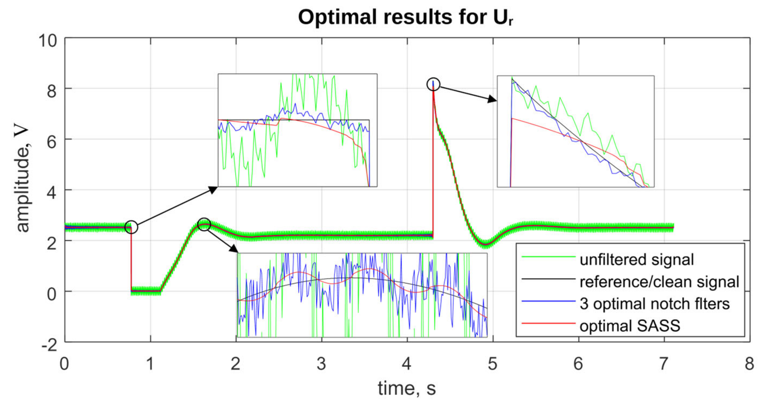
9.1. Regulator Output Voltage U_r

The optimization results for the LTI filters are presented in

Table 3. LTI filters optimization results for U_r (green—best results, orange—worst results).

	Errors and Goal Function Values			Low-Pass Filter		Notch Filter Width
Filtering Method	eRMS	eMAX	f	Order	fl, Hz	fw50, Hz	fw500, Hz	fw1000, Hz
No filtering	100%	100%	100%	-	-	-	-	-
Low-pass filter	87%	1381%	93%	1	86	-	-	-
3 notch filters	14%	48%	14%	-	-	0.48	2.6	6.5
3 notch + low-pass	14%	97%	14%	1	1500	0.48	2.4	4.6
2 notch + low-pass	18%	482%	21%	4	898	0.48	2.0	-
1 notch + low-pass	27%	962%	35%	4	449	0.48	-	-

. It can be observed that the lowest function goal value equal to 14% was achieved for three notch filters and three notches + low-pass filters of order 1. However, the designed low-pass filter cut-off frequency was equal to 1500 Hz, which is equal to the Nyquist frequency, so the filter does nothing except some antialiasing filtering and doubling the maximal error by lowering the steepness of the sharp slopes.

The worst results were achieved for the low-pass filter alone (goal function value equal to 93%), with the maximal error at a level equal to 1381% of the starting value. This shows that simple low-pass filtering is usually not a good idea in the case of signals with steep slopes. For similar reasons, the combination of notch filters and low-pass filters also leads to worse results than just the three notch filters alone. However, in this case, the notch filters (as narrow band filters) remove just the harmonic components without any influence on the noise outside the filters’ bands.

Table 4. SASS optimization results for U_r (green—best results, orange—worst results).

	Errors and Goal Function Values			SASS Parameters
Filtering Method	eRMS	eMAX	f	Derivative Order	Filter Order	fc, Hz	λ
No filtering	100%	100%	100%	-	-	-	-
Optimal SASS	11%	140%	11%	1	1	11	1.06
Optimal SASS	7%	110%	7%	1	2	20	1.11
Optimal SASS	40%	1261%	49%	2	1	21	7.52
Optimal SASS	40%	1259%	49%	2	2	32	7.67

presents the optimization results for the optimal SASS method. Best results were achieved for the first-order derivative and second-order filter. The lowest goal function value is equal to 7%, which is significantly better than the best LTI value, which is equal to 14%.

However, it is worth noting that the maximal error value in the case of the optimal SASS method is equal to 110%, and the lowest maximal error for LTI filters is equal to 48%. This can be explained by looking at the signals in the time domain (Figure 7).

One may observe, from Figure 7, that the maximal error for the optimal SASS method is evidently larger around the discontinuity points. On the other hand, the noise level in the SASS-filtered signal is definitely smaller in comparison to the notch filters’ case. Moreover, the optimal SASS method introduces some new removable discontinuity points, which are located in the places of the steepest parts of the signal (in this case, these are the harmonics “zero-crossing” points). This might suggest that the biggest problem for the SASS algorithm is not the noise level but the presence of harmonic components in the signal.

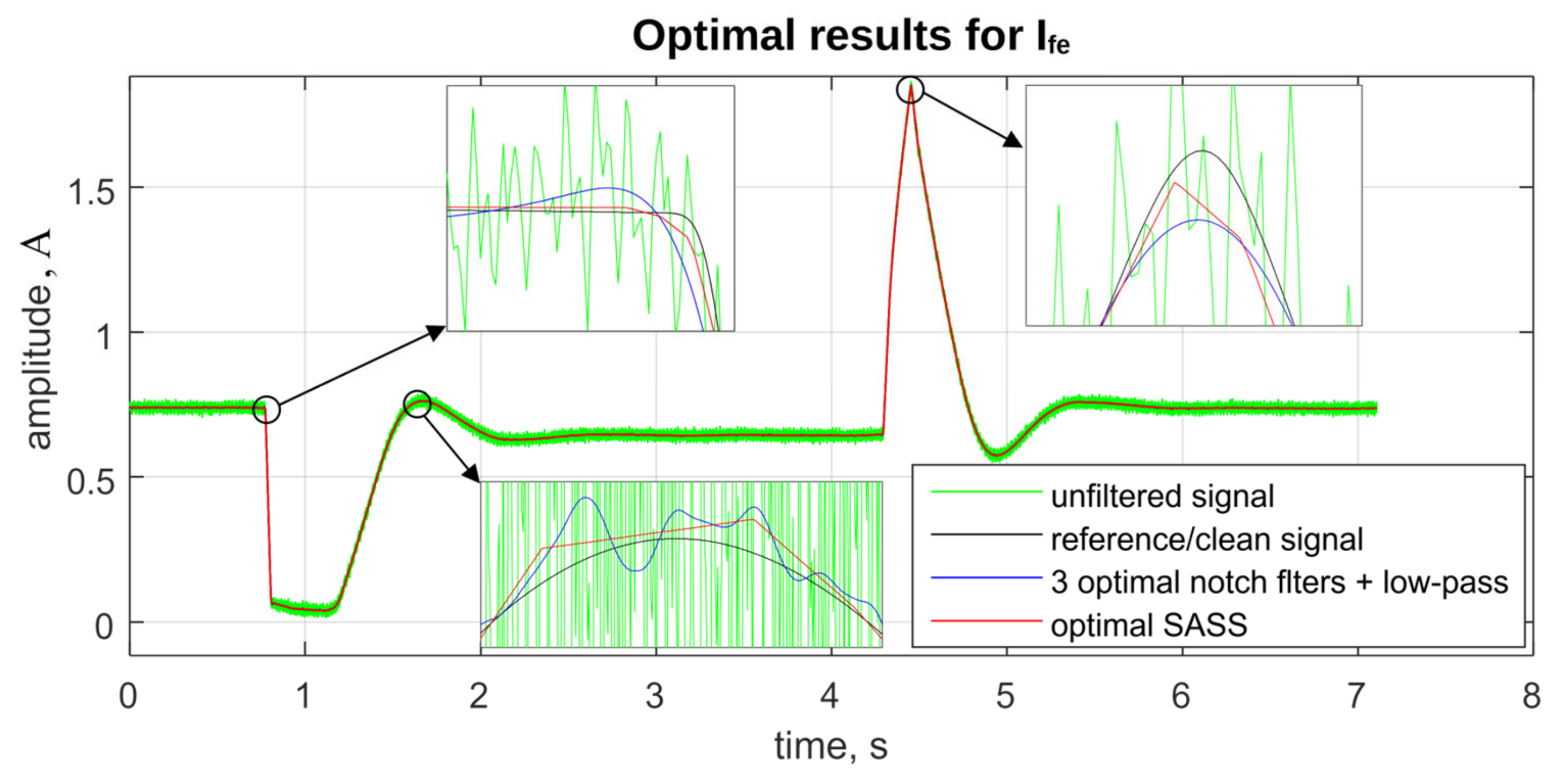
9.2. Exciter Field Current I_fe

The optimization results for the LTI filters are presented in

Table 5. TI filters optimization results for I_fe (green—best results, orange—worst results).

	Errors and Goal Function Values			Low-Pass Filter		Notch Filter Width
Filtering Method	eRMS	eMAX	f	Order	fl, Hz	fw50, Hz	fw500, Hz	fw1000, Hz
No filtering	100%	100%	100%	-	-	-	-	-
Low-pass filter	13%	68%	13%	4	38	-	-	-
3 notch filters	19%	28%	19%	-	-	2.18	983.3	986.0
3 notch + low-pass	9.8%	41.0%	9.9%	2	63	1.53	83.3	98.3
2 notch + low-pass	9.8%	42.5%	9.9%	2	61	1.40	115.5	-
1 notch + low-pass	9.8%	41.3%	9.9%	2	63	1.51	-	-

. The lowest function goal value equal to 9.9% was achieved for all combinations of notch filters with the addition of a low-pass filter. It is worth noting that among the best results with a goal function value equal to 9.9%, the lowest maximal error was achieved for three notch filters combined with a low-pass filter. On the other hand, the worst results with a goal function value equal to 19% were obtained for the three notch filters alone, which is a significantly different result in comparison with the U_r signal.

Table 6. SASS optimization results for I_fe (green—best results, orange—worst results).

	Errors and Goal Function Values			SASS Parameters
Filtering Method	eRMS	eMAX	f	Derivative Order	Filter Order	fc, Hz	λ
No filtering	100%	100%	100%	-	-	-	-
Optimal SASS	16.6%	63.9%	16.8%	1	1	21	0.07
Optimal SASS	12.8%	72.7%	13.0%	1	2	31	0.08
Optimal SASS	4.6%	21.5%	4.7%	2	1	1.86	3.82
Optimal SASS	4.8%	18.5%	4.8%	2	2	12	2.33

presents the optimization results for the optimal SASS method. The best results were achieved for the second-order derivative and first-order filter. The lowest goal function value is equal to 4.7%, which is significantly smaller than for the best LTI filters. It can also be noticed that for Ife, the maximal error is always smaller than 100%, unlike in the U_r case.

Figure 8 shows a comparison of signals after optimal LTI and optimal SASS filtering. It can be observed that for the optimal SASS method the noise and harmonics have been removed very efficiently.

However, the signal contains additional removable discontinuity points, which might be undesirable in some applications.

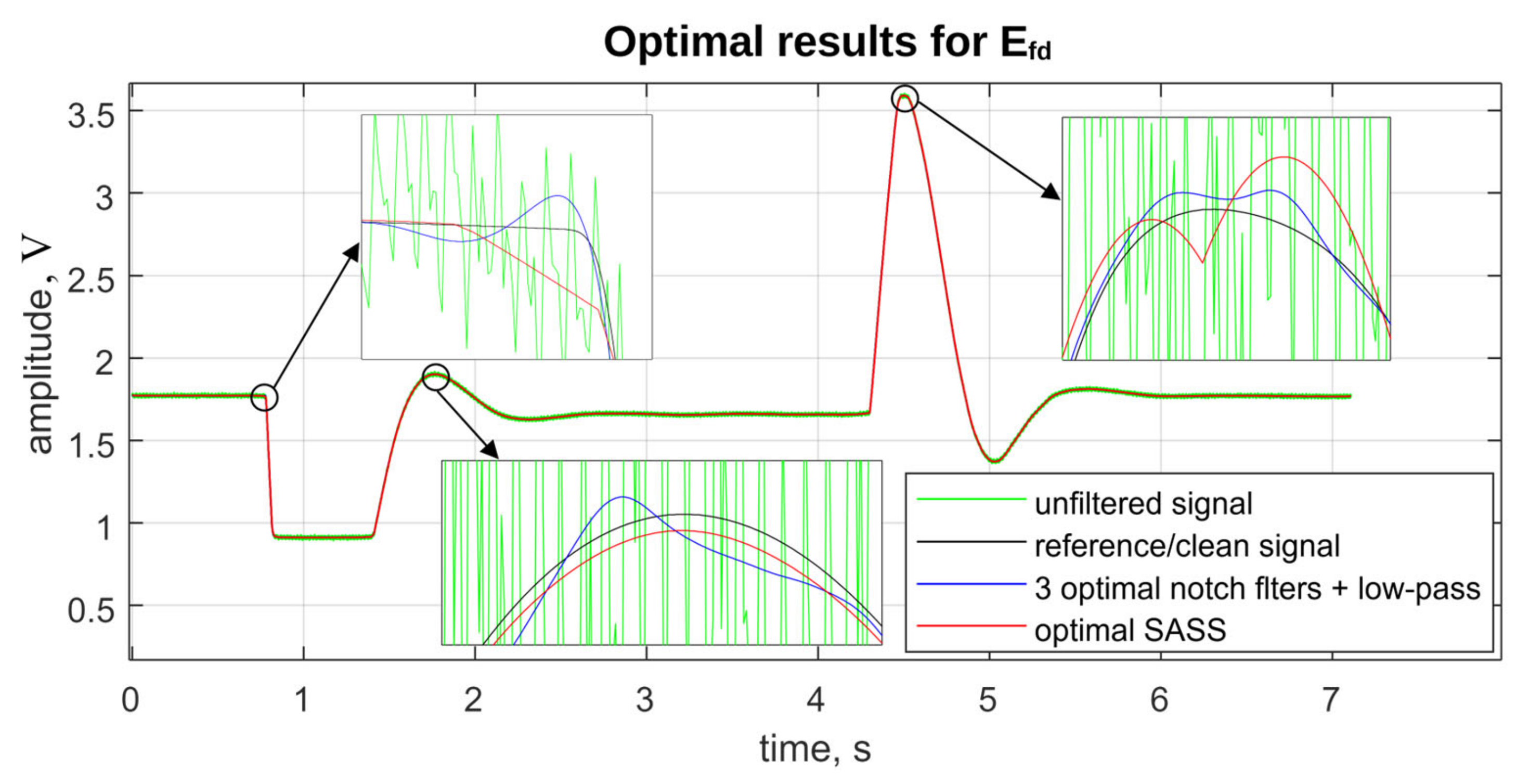
9.3. Generator Field Voltage E_fd

The optimization results for the LTI filters are presented in

Table 7. LTI filters optimization results for E_fd (green—best results, orange—worst results).

	Errors and Goal Function Values			Low-Pass Filter		Notch Filter Width
Filtering Method	eRMS	eMAX	f	Order	fl, Hz	fw50, Hz	fw500, Hz	fw1000, Hz
No filtering	100%	100%	100%	-	-	-	-	-
Low-pass filter	15%	80%	16%	4	40	-	-	-
3 notch filters	24%	29%	24%	-	-	2.1	303	381
3 notch + low-pass	8.9%	32.2%	8.99%	3	77	1.3	116	112
2 notch + low-pass	9.0%	30.3%	9.04%	3	82	1.5	119	-
1 notch + low-pass	8.9%	32.1%	9.00%	3	77	1.27	-	-

. The lowest function goal value equal to 8.99% was achieved for three notch filters combined with a low-pass filter, but the results are comparable for all notch + low-pass cases. The worst results with a goal function value equal to 24% were obtained for the three notch filters alone.

Table 8. SASS optimization results for E_fd (green—best results, orange—worst results).

	Errors and Goal Function Values			SASS Parameters
Filtering Method	eRMS	eMAX	f	Derivative Order	Filter Order	fc, Hz	λ
No filtering	100%	100%	100%	-	-	-	-
Optimal SASS	24.4%	96.6%	24.6%	1	1	32	0.04
Optimal SASS	14.5%	70.7%	14.7%	1	2	32	0.05
Optimal SASS	7.1%	25.0%	7.1%	2	1	0.41	2.23
Optimal SASS	6.8%	27.8%	6.9%	2	2	12	0.92

presents the optimization results for the optimal SASS method. This time, the best results were achieved for the second-order derivative and second-order filter. The lowest goal function value is equal to 6.9%, which is smaller than the best LTI solution. The worst result is achieved for the first-order derivative and first-order filter, and its level equal to 24.6% is comparable with the worst LTI result (goal function value equal to 24%).

Figure 9 shows a comparison of signals after optimal LTI and optimal SASS filtering. It can be observed that for both methods, some oscillations coming from the harmonic components are still present in the output signals.

The optimal SASS signal contains additional removable discontinuity points (Figure 9) in spite of its generally better performance in terms of evaluated error values.

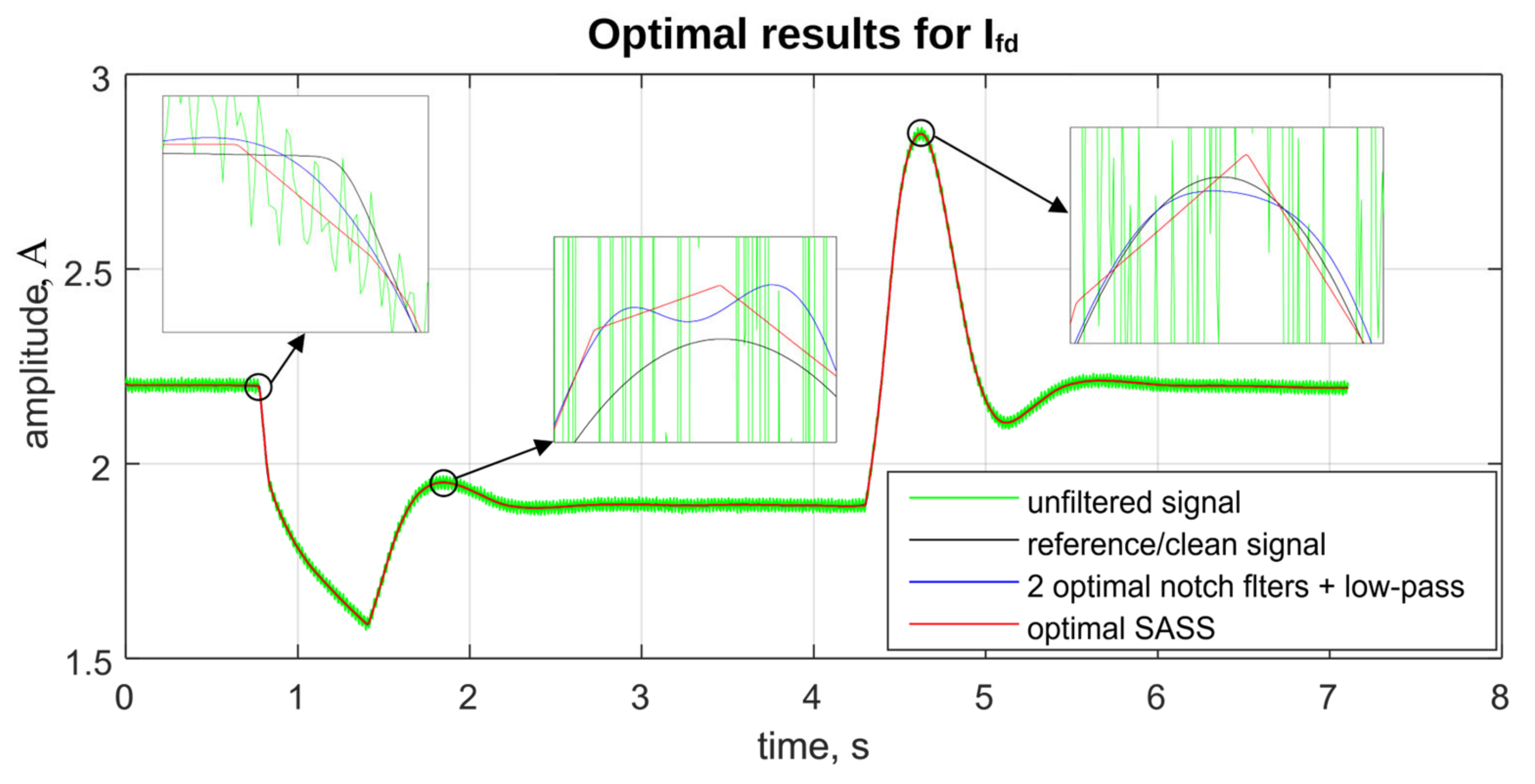
9.4. Generator Field Current I_fd

The optimization results for the LTI filters are presented in

Table 9. LTI filters optimization results for I_fd (green—best results, orange—worst results).

	Errors and Goal Function Values			Low-Pass Filter		Notch Filter Width
Filtering Method	eRMS	eMAX	f	Order	fl, Hz	fw50, Hz	fw500, Hz	fw1000, Hz
No filtering	100%	100%	100%	-	-	-	-	-
Low-pass filter	6%	35%	6%	3	26	-	-	-
3 notch filters	7%	37%	7%	-	-	13.0	998	999
3 notch + low-pass	5.0%	24.6%	5.1%	4	35	5.58	137	131
2 notch + low-pass	5.0%	23.7%	5.0%	3	37	3.20	69.2	-
1 notch + low-pass	5.0%	23.9%	5.1%	3	36	2.76	-	-

. The lowest function goal value equal to 5% was achieved for two notch filters combined with a low-pass filter. However, results for all notch filters + low-pass filters are very close. The worst results with a goal function value equal to 7% were obtained for the three notch filters alone. It is also worth noting that in this case, the 500 Hz and 1 kHz notches are very wide, so in fact, they are working as wide-band denoising filters. Such wide-width notch filters are not observed when the low-pass filter is added.

Table 10. SASS optimization results for I_fd (green—best results, orange—worst results).

	Errors and Goal Function Values			SASS Parameters
Filtering Method	eRMS	eMAX	f	Derivative Order	Filter Order	fc, Hz	λ
No filtering	100%	100%	100%	-	-	-	-
Optimal SASS	16.3%	71.6%	16.4%	1	1	19	0.10
Optimal SASS	7.2%	45.8%	7.4%	1	2	22	0.89
Optimal SASS	5.5%	39.2%	5.6%	2	1	0.34	4.52
Optimal SASS	6.0%	39.2%	6.1%	2	2	12	3.48

presents the optimization results for the optimal SASS method. The best results were achieved for the second-order derivative and first-order filter (similarly to I_fe). The lowest goal function value is equal to 5.6%, and this time, it is worse by about 0.5% than for the best LTI filter result. Also, the worst goal function value equal to 16.4% is much higher than the worst LTI result. Since the I_fd signal is generally significantly smoother than the Ife signal, it might suggest that the optimal SASS method might lead to better results only if signals are not “smooth enough”.

Figure 10 shows a comparison of signals after optimal LTI and optimal SASS filtering. Observably, optimal SASS again leads to removable discontinuities in places where the signals have steep slopes (it is around the largest harmonic component, “zero-crossing” points).

9.5. Summary of Optimization Results

Considering the evaluated errors and goal function values, in the case of I_fe and E_fd, the optimal SASS method produces better results in comparison with the optimal LTI filters. However, the situation is a bit more complicated for the U_r and I_fd signals.

In the case of the regulator voltage U_r, the maximal error was significantly smaller for optimal LTI filters (58%) as compared to optimal SASS (110%). At the same time, the corresponding RMS error is smaller for optimal SASS (7%) than for the optimal LTI filters (14%). It is important to mention that the optimal LTI result was achieved for three narrow-band notch filters (without the low-pass filter), which means that the optimal LTI case filters out just the harmonic components. On the other hand, the optimal SASS method works well when removing the noise component but finds it problematic to deal with the harmonic components (the removable discontinuity artifacts are introduced to the signal in the harmonic zero-crossing points).

In the case of the field current I_fd, all three parameters are better for the LTI method based on two notch filters combined with the low-pass filter. It means that for this particular signal, the low-pass filter does not affect the slopes significantly enough to let the optimal SASS method win. This suggests that for signals which can be considered “smooth enough”, a typical low-pass filter might be sufficient as a wide-band denoising filter.

Considering the optimal SASS method, it is also necessary to mention that in all considered optimal cases, some additional removable discontinuity points were introduced to the signals. This might lead to a conclusion that the removable discontinuity points are the typical artifacts that may appear when the SASS method is used. In some cases, these artifacts might be a serious problem (i.e., in a higher-order dynamical system modeling). On the other hand, the artifacts appear in the points with a high derivative value (in comparison to the rest of the signal), so they might be controlled by the regularization parameter.

It is also necessary to mention that some numerical stability problems (like bad matrix conditioning and very slow convergence) were experienced for the SASS implementation provided in [36]. It was perfectly stable for the first derivative and first-order filter, with sometimes much slower convergence and bad matrix conditioning for the second derivative and second-order filter, so there is definitely room for improvement in this field.

Considering the computational efficiency of the presented methods, it is worth mentioning that on a typical medium-class laptop, the computing time of the optimization procedure varies from a couple of seconds for the gradient algorithm and LTI filters to about 15 min for the optimal SASS method. When the optimal parameters are determined, the filtering alone is less than a minute, even for the optimal SASS algorithm, and a couple of seconds for LTI filters.

10. Summary and Conclusions

The performance of the optimal SASS method was evaluated for four transient signals recorded during a typical disturbance test of a 200 MW power-generating unit. It is difficult to remove noise and harmonic interference from these signals because of the discontinuities present in the signals. The optimal SASS results were compared with corresponding LTI filtering techniques like notch filtering and low-pass filtering, which use the same filter types (low-pass Butterworth filters) and the same zero-phase filtering principle as the SASS algorithm.

The measurement signals obtained during a power-generating unit test were carefully analyzed, and a mathematical model of the signals has been proposed.

Then, the optimal SASS method was proposed as well as the LTI filters (notch and low-pass), which were used as a reference point for the SASS method.

In the next step, the general optimization procedure for all tested methods was defined, the test signals were generated using the model of the generating unit and proposed signal model and a detailed performance evaluation of all considered filtering techniques was presented.

It has been shown that in the case of signals with wide-band noise and harmonic interferences, the proposed optimal SASS algorithm performance strongly depends on the signal shape. In some cases, traditional filtering techniques might lead to better performance in terms of evaluated errors. The optimal SASS method finds it difficult to deal with interference signals with a high derivative value (like the harmonic components zero-crossing points) but works very well for wideband noise rejection.

The SASS method can introduce characteristic artifacts, which are additional removable discontinuity points that are not present in the original signal. These artifacts appear at points where the considered derivative value is high enough. This behavior can be controlled by increasing the regularization parameter λ; however, this leads to worse interference rejection.

To summarize, the SASS and proposed optimal SASS methods might be a valuable tool in transient signal denoising but should be used carefully because of possible artifacts introduced into the signal. When the signal contains interferences other than noise (e.g., harmonic components), then the assistance of other filtering methods might be a good idea.

11. Future Work

Future work will be focused on removing the weak points of the SASS method (like the artifacts) and improving its performance in power system signals denoising.

The next step is a direct continuation of the comparison presented in this paper and is inspired by the conclusions from the previous section. Paper [22] proposes a new method, which is a combination of notch filters for harmonic rejection and the SASS method for noise removal. It has been shown in [22] that this new method leads to superior results in comparison with the best results examined in detail in the present paper.

It is also very important to notice here that (due to unfortunate timing) it was impossible to cite the present paper in [22] because [22] was already published while the present paper was still in the reviewing process. Since we used exactly the same methodology in both papers to make the results directly comparable and citation was not possible, we were forced to show the background of the methods in both papers (introduction, LTI filters, and SASS description, as well as the signals and optimization strategy description); however, these sections were rewritten and adjusted to the paper content in each paper accordingly (they are not direct citations). To make things as clear as possible, we have added references to [22] in the present paper even if, chronologically, it is the first paper that should be published.

References

1. Jiang, H.; Zhang, Y.; Muljadi, E. New Technologies for Power System Operation and Analysis; Jiang, H., Zhang, Y., Muljadi, E., Eds.; Academic Press: Cambridge, MA, USA, 2021. [Google Scholar]
2. Sodhi, R. Simulation and Analysis of Modern Power Systems; McGraw Hill Education: New York, NY, USA, 2021. [Google Scholar]
3. Goud, B.S.; Kalyan, C.N.S.; Rao, G.S.; Reddy, B.N.; Kumar, Y.A.; Reddy, C.R. Combined LFC and AVR Regulation of Multi Area Interconnected Power System Using Energy Storage Devices. In Proceedings of the IEEE 2nd International Conference on Sustainable Energy and Future Electric Transportation (SeFeT), Hyderabad, India, 4–6 August 2022; pp. 1–6. [Google Scholar]
4. Machowski, J.; Lubośny, Z.; Białek, J.; Bumby, J. Power System Dynamics: Stability and Control, 3rd ed.; Wiley: Hoboken, NJ, USA, 2020; pp. 1–888. [Google Scholar]
5. Vittal, V.; McCalley, J.D.; Anderson, P.M.; Fouad, A.A. Power System Control and Stability, 3rd ed.; Wiley-IEEE Press: Hoboken, NJ, USA, 2019; p. 832. [Google Scholar]
6. Paszek, S.; Boboń, A.; Berhausen, S.; Majka, Ł.; Nocoń, A.; Pruski, P. Synchronous Generators and Excitation Systems Operating in a Power System: Measurement Methods and Modelling; Lecture Notes in Electrical Engineering; Springer: Cham, Switzerland, 2020; p. 631. [Google Scholar]
7. Majka, Ł.; Baron, B.; Zydroń, P. Measurement-based stiff equation methodology for single phase transformer inrush current computations. Energies 2022, 15, 7651. [Google Scholar] [CrossRef]
8. IEEE Std 421.5—2016; IEEE Recommended Practice for Excitation System Models for Power System Stability Studies. Energy Development and Power Generation Committee of the IEEE Power and Energy Society: New York, NY, USA, 2016.
9. Máslo, K.; Kasembe, A. Extended long term dynamic simulation of power system. In Proceedings of the 52nd International Universities Power Engineering Conference (UPEC), Heraklion, Greece, 28–31 August 2017; pp. 1–5. [Google Scholar]
10. Verrelli, C.M.; Marino, R.; Tomei, P.; Damm, G. Nonlinear Robust Coordinated PSS-AVR Control for a Synchronous Generator Connected to an Infinite Bus. IEEE Trans. Autom. Control. 2022, 67, 1414–1422. [Google Scholar] [CrossRef]
11. Imai, S.; Novosel, D.; Karlsson, D.; Apostolov, A. Unexpected Consequences: Global Blackout Experiences and Preventive Solutions. IEEE Power Energy Mag. 2023, 21, 16–29. [Google Scholar] [CrossRef]
12. Almas, M.S.; Vanfretti, L. RT-HIL Testing of an Excitation Control System for Oscillation Damping using External Stabilizing Signals. In Proceedings of the IEEE Power & Energy Society General Meeting, Denver, CO, USA, 26–30 July 2015. [Google Scholar]
13. Reliability Guideline: Power Plant Model Verification and Testing for Synchronous Machines; North American Electric Reliability Corporation (NERC): Atlanta, GA, USA, 2018; p. 30326.
14. Dynamic Model Acceptance Test Guideline; Version 2; Australian Energy Market Operator Limited (AEMO): Melbourne, Australia, 2021.
15. Bérubé, G.R.; Hajagos, L.M. Testing & Modeling of Generator Controls; KESTREL POWER ENGINEERING, ENTRUST Solutions Group: Warrenville, IL, USA, 2003. [Google Scholar]
16. Pruski, P.; Paszek, S. Location of generating units most affecting the angular stability of the power system based on the analysis of instantaneous power waveforms. Arch. Control. Sci. 2020, 30, 273–293. [Google Scholar] [CrossRef]
17. IEEE Std 421.2—2014; IEEE Guide for Identification, Testing, and Evaluation of the Dynamic Performance of Excitation Control Systems. Energy Development and Power Generation Committee of the IEEE Power and Energy Society: New York, NY, USA, 2014.
18. Monti, A.; Benigni, A. Modeling and Simulation of Complex Power Systems; Institution of Engineering and Technology (IET): Stevenage, UK, 2022; p. 320. [Google Scholar]
19. Máslo, K.; Kasembe, A.; Kolcun, M. Simplification and unification of IEEE standard models for excitation systems. Electr. Power Syst. Res. 2016, 140, 132–138. [Google Scholar] [CrossRef]
20. Majka, Ł. Using fractional calculus in an attempt at modeling a high frequency AC exciter. In Advances in Non-Integer Order Calculus and Its Applications, Proceedings of the 10th International Conference on Non-Integer Order Calculus and Its Applications, Bialystok, Poland, 20–21 September 2018; Lecture Notes in Electrical Engineering; Springer: Berlin/Heidelberg, Germany, 2020; Volume 559, pp. 55–71. [Google Scholar]
21. Sowa, M.; Majka, Ł.; Wajda, K. Excitation system voltage regulator modeling with the use of fractional calculus. AEU Int. J. Electron. Commun. 2023, 159, 154471. [Google Scholar] [CrossRef]
22. Lewandowski, M.; Majka, Ł. Combining optimal SASS (Sparsity Assisted Signal Smoothing) and notch filters for transient measurement signals denoising of large power generating unit. Measurement 2024, 237, 115174. [Google Scholar] [CrossRef]
23. Pruski, P.; Paszek, S. Calculations of power system electromechanical eigenvalues based on analysis of instantaneous power waveforms at different disturbances. Appl. Math. Comput. 2018, 319, 104–114. [Google Scholar] [CrossRef]
24. Lewandowski, M.; Majka, Ł.; Świetlicka, A. Effective estimation of angular speed of synchronous generator based on stator voltage measurement. Int. J. Electr. Power Energy Syst. 2018, 100, 391–399. [Google Scholar] [CrossRef]
25. Układy Rejestracji—Kared Sp. z o.o. Oficjalna Strona Firmy. Available online: https://kared.pl/produkty/uklady-rejestracji/ (accessed on 30 May 2024).
26. Micev, M.; Ćalasan, M.; Stipanović, D.; Radulović, M. Modeling the relation between the AVR setpoint and the terminal voltage of the generator using artificial neural networks. Eng. Appl. Artif. Intell. 2023, 120, 105852. [Google Scholar] [CrossRef]
27. How to Perform a Step Test. Control Station, Inc., 642 Hilliard Street, Suite 2301, Manchester, Connecticut 06042, United States. 19 July 2016. Available online: https://controlstation.com/blog/perform-step-test/ (accessed on 30 May 2024).
28. Kumar, K.; Singh, A.K.; Singh, R.P. Power System Stabilization Tuning and Step Response Test of AVR: A Case Study. In Proceedings of the 6th International Conference on Advanced Computing and Communication Systems (ICACCS), Coimbatore, India, 6–7 March 2020; pp. 482–485. [Google Scholar]
29. Energotest Sp. z o.o., Cyfrowe Układy Wzbudzenia i Regulacji Napięcia Typu ETW. Available online: https://www.spie-energotest.pl/media/k-etw.pdf (accessed on 30 May 2024).
30. Bethoux, O. PID Controller Design, Encyclopedia of Electrical and Electronic Power Engineering; Elsevier: Amsterdam, The Netherlands, 2023; pp. 261–267. [Google Scholar]
31. Bingul, Z.; Karahan, O. A novel performance criterion approach to optimum design of PID controller using cuckoo search algorithm for AVR system. J. Frankl. Inst. 2018, 355, 5534–5559. [Google Scholar] [CrossRef]
32. Jumani, T.A.; Mustafa, M.W.; Hussain, Z.; Rasid, M.M.; Saeed, M.S.; Memon, M.M.; Khan, I.; Nisar, K.S. Jaya optimization algorithm for transient response and stability enhancement of a fractional-order PID based automatic voltage regulator system. Alex. Eng. J. 2020, 59, 2429–2440. [Google Scholar] [CrossRef]
33. Tan, L.; Jiang, J. Digital Signal Processing Fundamentals and Applications, 3rd ed.; Elsevier: Amsterdam, The Netherlands, 2019. [Google Scholar]
34. Fan, G.; Li, J.; Hao, H. Vibration signal denoising for structural health monitoring by residual convolutional neural networks. Measurement 2020, 157, 107651. [Google Scholar] [CrossRef]
35. Tian, C.; Fei, L.; Zheng, W.; Xu, Y.; Zuo, W.; Lin, C.-W. Deep learning on image denoising: An overview. Neural Netw. 2020, 131, 251–275. [Google Scholar] [CrossRef] [PubMed]
36. Selesnick, I. Sparsity-assisted signal smoothing (revisited). In Proceedings of the IEEE International Conference on Acoustics, Speech and Signal Processing (ICASSP), New Orleans, LA, USA, 5–9 March 2017; pp. 4546–4550. [Google Scholar]
37. Niedźwiecki, M.; Ciołek, M. Fully Adaptive Savitzky-Golay Type Smoothers. In Proceedings of the 27th European Signal Processing Conference (EUSIPCO), A Coruna, Spain, 2–6 September 2019; pp. 1–5. [Google Scholar]
38. Kozlowski, B. Time series denoising with wavelet transform. J. Telecommun. Inf. Technol. 2005, 3, 91–95. [Google Scholar] [CrossRef]
39. Chatterjee, S.; Thakur, R.S.; Yadav, R.N.; Gupta, L.; Raghuvanshi, D.K. Review of noise removal techniques in ECG signals. IET Signal Process. 2020, 14, 569–590. [Google Scholar] [CrossRef]
40. Selesnick, I.W.; Arnold, S.; Dantham, V.R. Polynomial Smoothing of Time Series With Additive Step Discontinuities. IEEE Trans. Signal Process. 2012, 60, 6305–6318. [Google Scholar] [CrossRef]
41. Savitzky, A.; Golay, M.J.E. Smoothing and Differentiation of Data by Simplified Least Squares Procedures. Anal. Chem. 1964, 36, 1627–1639. [Google Scholar] [CrossRef]
42. Vetterli, M.; Cormac, H. Wavelets and Filter Banks: Theory and Design. IEEE Trans. Signal Process. 1992, 40, 2207–2232. [Google Scholar] [CrossRef]
43. Orfanidis, S.J. Introduction to Signal Processing; Prentice Hall Inc.: Saddle River, NJ, USA, 2009; Chapter 6, Section 6.4.3. [Google Scholar]
44. Parks, T.W.; Burrus, C.S. Digital Filter Design; John Wiley & Sons: Hoboken, NJ, USA, 1987; Chapter 7, Section 7.3.3. [Google Scholar]
Figure 1. Schematic diagram of a considered 200 MW type generating unit.
Energies 17 04976 g001
Figure 2. The waveforms recorded in response to a step change in the voltage regulator’s reference voltage Uref [22].
Energies 17 04976 g002
Figure 3. The amplitude spectrum of the recorded waveforms [22].
Energies 17 04976 g003
Figure 4. Reference LTI filtering method.
Energies 17 04976 g004
Figure 5. Distorted UrP signal (with noise and harmonic components) generated from the model of the generating unit [22].
Energies 17 04976 g005
Figure 6. Diagram of the optimization method [22].
Energies 17 04976 g006
Figure 7. Comparison of optimal SASS- and LTI-filtered signals in the time domain.
Energies 17 04976 g007
Figure 8. Comparison of optimal SASS- and LTI-filtered signals in the time domain.
Energies 17 04976 g008
Figure 9. Comparison of optimal SASS- and LTI-filtered signals in the time domain.
Energies 17 04976 g009
Figure 10. Comparison of optimal SASS- and LTI-filtered signals in the time domain.
Energies 17 04976 g010