Thermodynamics-Informed Neural Networks for the Design of Solar Collectors: An Application on Water Heating in the Highland Areas of the Andes

Abstract

This study addresses the challenge of optimizing flat-plate solar collector design, traditionally reliant on trial-and-error and simplified engineering design methods. We propose using physics-informed neural networks (PINNs) to predict optimal design conditions in a range of data that not only characterized the highlands of Ecuador but also similar geographical locations. The model integrates three interconnected neural networks to predict global collector efficiency by considering atmospheric, geometric, and physical variables, including overall loss coefficient, efficiency factors, outlet fluid temperature, and useful heat gain. The PINNs model surpasses traditional simplified thermodynamic equations employed in engineering design by effectively integrating thermodynamic principles with data-driven insights, offering more accurate modeling of nonlinear phenomena. This approach enhances the precision of solar collector performance predictions, making it particularly valuable for optimizing designs in Ecuador’s highlands and similar regions with unique climatic conditions. The ANN predicted a collector overall loss coefficient of 5.199 W/(m²·K), closely matching the thermodynamic model’s 5.189 W/(m²·K), with similar accuracy in collector useful energy gain (722.85 W) and global collector efficiency (33.68%). Although the PINNs model showed minor discrepancies in certain parameters, it outperformed traditional methods in capturing the complex, nonlinear behavior of the data set, especially in predicting outlet fluid temperature (55.05 °C vs. 67.22 °C).

1. Introduction

In an era where the dialogue on climate action shifted from mere awareness to urgent implementation, the study of renewable energy sources, particularly solar energy, assumes critical importance [1,2,3]. Solar energy, harnessed for electricity production and water heating, presents a feasible alternative in the quest to mitigate the global rise in fossil fuel demand and the associated environmental degradation [4]. The current research pivots on to assess the influence of the design parameters of flat-plate solar collectors in the overall efficiency of the collector through the lens of thermodynamics-informed artificial neural networks (ANN) in order to improve the efficiency of solar collectors, offering a synergy between traditional engineering design and advanced machine learning concepts [5].

The utilization of solar thermal systems aligns closely with international energy management policies, and notably, with those developing within the Ecuadorian energy policy [6,7]. Despite the country’s advantageous equatorial position, which promises abundant solar radiation, the integration of solar power into the national energy portfolio is limited due to economical, social, and political reasons; consequently, there is limited infrastructure that takes advantage of solar energy alternatives [8]. Recent governmental initiatives indicate a paradigm shift towards incorporating solar power as a key renewable resource [9]. This strategic move focuses on reducing reliance on fossil fuel, leading to the improvement of air quality, and thereby supporting the sustainable development goals [10].

Previous studies explored various methods to enhance the efficiency of solar water heaters, focusing on distinct physical characteristics that contribute to system performance. For instance, Riffat et al. [11] investigate the impact of the inner fluid’s thermal properties on the overall heat transfer efficiency within solar collectors, emphasizing how fluid composition can significantly influence energy absorption and retention. In another study, Shariah et al. [12] examine the optimal tilt angle for solar collectors, providing detailed analysis on how geographical location and seasonal variations affect incident solar radiation, and thus, collector performance. Additionally, Recalde et al. [13] analyze fluid circulation patterns across tube collectors, highlighting the importance of flow rate and uniform distribution in maximizing thermal efficiency. Each of these studies underscores the complexity of optimizing solar collectors through experimental methods, which often involves managing numerous interdependent variables simultaneously. This inherent complexity makes the experimental trial-and-error approach laborious and time-consuming, thus delaying advancements in solar collector technology.

To address the limitations of traditional optimization methods, recent research increasingly focused on utilizing ANNs for enhancing the performance of solar collectors [14]. While this represents significant progress, existing studies never fully exploited the potential of ANNs to optimize design parameters for maximizing thermal efficiency. Moreover, a critical gap exists in the literature regarding the consideration of region-specific climatic conditions, such as those in Ecuador, which play a pivotal role in the performance of solar collectors.

A thorough review of the literature reveals several key insights. Yaici et al. (2015) [15] demonstrated the effectiveness of ANNs in predicting the performance of solar thermal systems under varying climatic conditions, reinforcing the need for region-specific models. Kalogirou (2003) [16] similarly highlighted the potential of ANNs to optimize solar collector efficiency by incorporating diverse environmental factors. However, despite these promising developments, current research never sufficiently integrated ANN models to optimize thermal efficiency design parameters in the unique climatic context of Ecuador. Furthermore, the literature lacks a comprehensive approach that integrates thermodynamic principles into ANN frameworks to address the specific performance variations caused by Ecuador’s climatic conditions. This gap in region-specific modeling and the lack of thermodynamics-informed ANN optimization forms the foundation of this study. Existing research lacks comprehensive approaches that integrate thermodynamic principles into ANN frameworks to account for the specific performance variations in solar collectors under Ecuador’s climatic conditions. This gap, particularly in region-specific modeling and thermodynamics-informed ANN optimization, is addressed by this study through the use of physics-informed neural networks. By combining deterministic thermodynamic processes with data-driven insights, PINNs offer a potential solution for modeling complex, nonlinear behaviors often oversimplified in conventional approaches, improving predictive accuracy for solar collectors in the Ecuadorian highlands.

The present research, therefore, seeks to bridge these gaps by employing ANN methodologies to evaluate the influence of components on thermal efficiency and thus be able to quickly optimize the design of flat plate solar collectors. This approach is not only innovative, but resonates with the need for computational models that can replicate complex systems, thereby reducing the need for extensive physical testing and the associated costs.

The implications of this research are twofold: firstly, to affirm the validity of ANN as a method for enhancing the design and efficiency of solar collectors; and secondly, to tailor this method to the specific environmental conditions of Ecuador. The outcomes of this study are anticipated to extend beyond theoretical contributions, opening scope to practical applications and design frameworks that can be implemented within a similar Ecuadorian context and that could serve for solar collector studies [17,18], thereby exemplifying a tailored approach to renewable energy design methods.

The research addresses the following key questions:

• How can ANN methodologies be applied to optimize the design parameters of flat-plate solar collectors for improved thermal efficiency?
• What impact do the specific climatic conditions of Ecuador have on the performance of solar collectors, and how can these be integrated into ANN models for enhanced design optimization?

By incorporating artificial neural networks into the design process, this study addresses the inherent nonlinearities in solar collector performance, which are often challenging to capture using purely analytical or empirical models. In particular, physics-informed neural networks are lever-aged to not only account for these nonlinear behaviors, but also to integrate thermodynamic equations directly into the model. This combined approach allows for a more accurate prediction of key parameters, such as temperature and efficiency, ultimately optimizing the solar collector design. Focusing on Ecuador’s unique climatic conditions further enhances the study’s relevance, providing region-specific solutions for improving the thermal efficiency of solar collectors. This dual contribution, both to theoretical advancements in modeling and to practical engineering applications, positions the research as impactful for the development of tailored solar energy solutions in diverse environmental contexts.

1.1. Artificial Neural Networks

Artificial neural networks represent a cornerstone of computational science, inspired by the biological neural networks that constitute animal brains [19]. At their core, ANNs are systems of interconnected nodes, or “neurons”, which process data inputs through a series of transformations to produce outputs. The strengths of these connections, known as weights, are adjusted during the training process to minimize the discrepancy between the ANN’s output and the known data, a process facilitated by a loss function [20]. This function quantifies the error of the network’s predictions, guiding the optimization algorithm, often a variant of gradient descent, to adjust the weights in a direction that reduces the loss [21].

Generalization, the ability of an ANN to perform well on unseen data, is a hallmark of a well-trained network. This aspect is particularly critical, as it determines the network’s utility in practical applications [22,23]. To avoid overfitting, or the memorization of training data at the expense of generalization, techniques such as regularization are employed, where additional constraints or penalties are introduced to the learning process. Activation functions imbue the network with non-linearity, allowing it to capture complex patterns. The bias term in each neuron is akin to an intercept in linear regression, enabling the neuron to fit the data better [24]. In the context of engineering design, the implications of ANNs are profound. They offer a paradigm shift from traditional deterministic or empirical design methodologies to data-driven, adaptive approaches. In design processes, ANNs can analyze complex data sets, recognize patterns, and make predictions or decisions with high accuracy [25]. They facilitate the exploration of vast design spaces, optimize performance criteria, and can even lead to the discovery of novel design principles or configurations. The application of ANNs to engineering design transcends mere automation; it is a transformative tool that enables engineers to harness the power of data and computation to innovate and solve problems with unprecedented efficiency and creativity [26].

Beyond this description, the proposed artificial neural network is not merely an abstract computational model; it is also designed to mirror the physical laws that govern solar collectors in the highland regions of the Andes of Ecuador [27]. Our approach is grounded in a theoretical thermodynamics’ framework, which was utilized to generate synthetic data sets. These data sets encapsulate the nuanced dynamics of solar energy conversion and the thermal behavior characteristic of high-altitude environments. By integrating this theoretical underpinning into the training of our ANN, we ensure that the model’s predictions are not only data-driven, but also physics-informed, a key characteristic of the proposed ANN-based model.

This synergy between computational intelligence and thermodynamic principles enhances the ANN’s predictive capabilities, ensuring that the model accurately reflects real-world physical interactions [28]. It allows the ANN to anticipate the performance of solar collectors with high precision, considering variables such as solar irradiance, ambient temperature, and material properties that are specific to the Andean highland context. Consequently, the ANN becomes a powerful tool for designing solar collectors, providing engineers with a data-driven yet physically anchored methodology. This method is expected to yield designs that are not only optimized for efficiency, but also contextualized to the unique environmental conditions of the Andes, thus contributing to engineering practices in renewable energy systems.

1.2. Physics-Informed Neural Networks

Physics-informed neural networks (PINNs) represent an innovative fusion of deep learning with the physical principles governing phenomena of interest in science and engineering [29,30]. Physics-informed neural networks: A deep learning framework for solving forward and inverse problems involving nonlinear partial differential equations. This approach integrates physical laws and principles, typically expressed in the form of equations or data, directly into one or more stages of the neural network model generation process.

By doing so, PINNs not only learn from available data, but also incorporate prior knowledge about the underlying behavior of the system they are modeling. This allows them to make more accurate predictions and better generalize to unseen situations, even with limited or noisy data sets.

The applications of PINNs are vast, spanning from fluid dynamics to structural engineering and particle physics, offering a powerful tool to solve complex problems where physical knowledge is crucial.

The stages in the neural network modeling process are described below [30]:

• Defining the Problem: what we are modeling.
• Curating Data: what data will inform the model.
• Designing the Neural Network Architecture: layers and activation functions.
• Defining an Optimization Function: loss function.
• Optimization.

To create a physics-informed neural network (PINN) based on the provided stages of a conventional ANN modelling process, we can introduce physics concepts and constraints at any of the steps [28].

2. Method

The strategy used in this study to introduce the physics of the problem focuses on the problem definition and data stages that inform the neural network model. The data are generated from mathematical models based on thermodynamic principles that allow for training the network and establishing fundamental parameters for the design of solar collectors in high Andean zones.

2.1. Conceptual PINN Model for the Design of Solar Collectors

2.1.1. Step 1. The Problem: What Are We Modeling?

Harnessing the computational power of artificial neural networks, we delve into a detailed analysis of flat-plate solar collectors with a focus on water heating applications. The predictive analytics derived from ANNs are vital in advancing the efficiency prediction of solar collectors, which is a significant step toward bolstering the sustainability of urban infrastructure.

To concretize the utility of ANNs, we apply them to refine the design of flat-plate solar collectors. These devices are crucial in the transformation of solar energy into heat and their performance is subject to wide fluctuations due to varying environmental conditions [11]. The capacity of ANNs to assimilate and learn from these environmental parameters, and to dynamically fine-tune operational factors, is instrumental in achieving marked enhancements in the prediction of global collector efficiency.

In our approach, we encapsulate the fundamental physics governing solar collectors within a synthetic data set derived from a comprehensive thermodynamic framework [31]. This data set informs or feeds into our neural network model, enabling it to internalize the underlying physical phenomena [30]. Consequently, the ANN is not only trained on empirical data, but is also steeped in the theoretical principles of solar energy conversion. Leveraging this hybrid model, we extract critical design parameters for the solar collectors, thus bridging the gap between theoretical physics and practical engineering design.

This revision adds clarity on the integration of thermodynamic principles with ANN (i.e., PINN model) training and the goal of obtaining design parameters, providing a comprehensive view of the modeling problem and the methodology applied to address it.

Engineering design requires that the dimensions and materials of a solar collector be optimized for maximum efficiency, cost-effectiveness, and alignment with existing infrastructure standards. Achieving the optimal temperature for residential hot water, typically ranging between 55 and 70 degrees Celsius [32], necessitates reliable performance under varying regional climatic conditions. Figure 1 illustrates the essential components of a flat-plate solar collector, highlighting the crucial elements that ensure its effective design and operation.

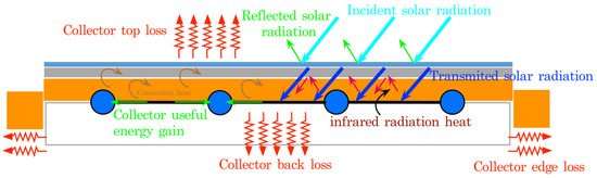
Figure 1. Flat-plate collector: thermodynamic description.

Figure 1. Flat-plate collector: thermodynamic description.

2.1.2. Step 2. The Neural Network Architecture: A Thermodynamics-Based Approach

The thermodynamic characterization of solar collectors follows the foundational models described in the previous sections [7,11,31]. These models are integral to the neural system’s development for predicting and optimizing the performance of solar thermal systems (Figure 2). A critical aspect of this characterization is the convective heat transfer coefficient between the collector’s tube and the fluid, which was computed using dimensionless parameters.

The thermal equilibrium in the water heating process via solar energy is quantified by the equation:

$${\mathrm{H}}_{\mathrm{T}}{\mathrm{A}}_{\mathrm{e}}={ \mathrm{H}}_{\mathrm{T}}{\mathrm{A}}_{\mathrm{e}}\left(1-{\left(\mathsf{\alpha }·\tau \right)}_{\mathrm{e}}\right)+{\mathrm{Q}}_{\mathrm{u}}+{\mathrm{Q}}_{\mathrm{l}}+{\displaystyle \frac{\partial \mathrm{V}}{\partial \mathrm{t}}}$$

(1)

where ${\mathrm{H}}_{\mathrm{T}}{\mathrm{A}}_{\mathrm{e}}$ is the incident solar radiation, ${\mathrm{H}}_{\mathrm{T}}$ global solar irradiation, ${\mathrm{A}}_{\mathrm{e}}$ plate area, ${\mathrm{H}}_{\mathrm{T}}{\mathrm{A}}_{\mathrm{e}}\left(1-{\left(\mathsf{\alpha }·\tau \right)}_{\mathrm{e}}\right)$ is the reflected solar radiation, ${\mathrm{Q}}_{\mathrm{u}}$ collector useful energy gain, ${\mathrm{Q}}_{\mathrm{l}}$ heat loss, ${\displaystyle \frac{\partial \mathrm{V}}{\partial \mathrm{t}}}$ stored heat, $\mathsf{\alpha }$ plate absorptance, and $\tau$ cover transmittance. Based on this fundamental thermodynamic balance equation, three interconnected neural network models were developed (Figure 3). These models, along with corresponding data sets for training, validation, and testing, were executed sequentially to map specific solar collector design parameters.

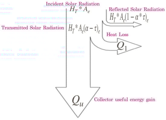
Figure 2. Flat-plate collector: thermodynamic balance. * It represents the energy balance depicted in Equation (1).

Figure 2. Flat-plate collector: thermodynamic balance. * It represents the energy balance depicted in Equation (1).

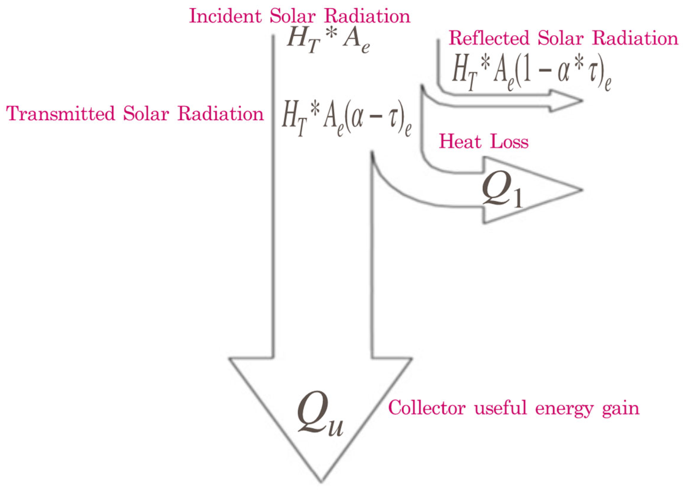
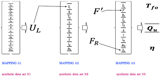
Figure 3. Conceptual diagram used in data generation and modeling based on ANN. The figure shows the conceptual structure used for the generation of synthetic data informed by thermodynamic principles. Each ANN is associated with a sequential generalization task. These mappings represent specific tasks or outputs that each network is designed to perform or predict based on its respective training data.

Figure 3. Conceptual diagram used in data generation and modeling based on ANN. The figure shows the conceptual structure used for the generation of synthetic data informed by thermodynamic principles. Each ANN is associated with a sequential generalization task. These mappings represent specific tasks or outputs that each network is designed to perform or predict based on its respective training data.

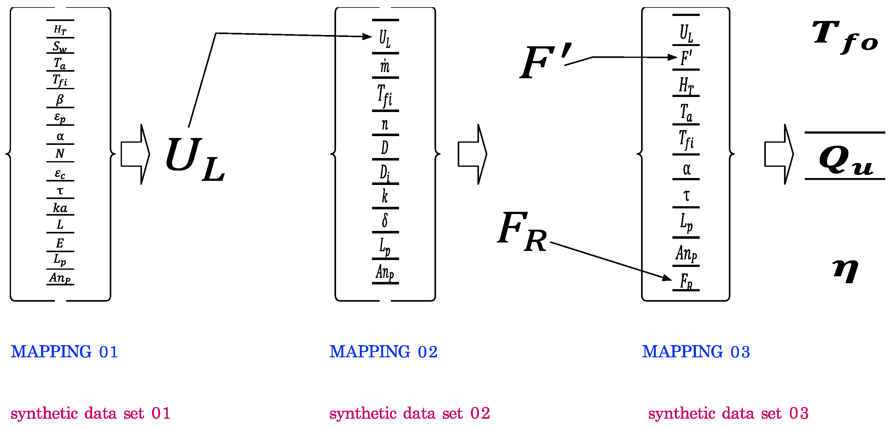
ANN 01: The Environmental and Solar Radiation-Informed ANN Model

The first ANN model (ANN 01) maps a set of variables to the collector overall coefficient. The variables under consideration form a comprehensive set that is crucial for optimizing the design and performance of solar collectors through the proposed ANN modeling. These parameters include environmental factors such as global solar irradiation, wind speed, and ambient temperature, which directly affect the energy capture and thermal dynamics of the system. The design-specific variables, such as the collector tilt, plate emittance, and absorptance, along with the physical dimensions of the plate, play pivotal roles in maximizing the efficiency of solar radiation absorption and minimizing heat loss. Additionally, the characteristics of the cover, including the number of covers, their emittance, transmittance, and the insulation properties (thermal conductivity, along with lower and lateral insulation thickness), are integral in managing the thermal insulation of the system. Together, these variables enable precise modelling of solar collector systems to enhance their effectiveness and adaptability to various environmental conditions and design requirements, fostering more sustainable and efficient energy solutions. The set of variables is used for the prediction of the collector overall loss coefficient.

ANN 02: The Design and Operational Efficiency-Informed ANN Model

The second mapping (ANN 02) facilitates the prediction of critical factors such as collector heat removal and collector efficiency, which are integral to the design process of solar collectors. This set of variables, crucial for both design and operational efficiency, includes the collector overall loss coefficient, indicating the rate of heat loss per unit area and temperature difference, essential for assessing thermal performance. Additionally, the mass flow rate is key for optimizing fluid dynamics within the system, ensuring efficient heat transfer. The configuration of the number of parallel tubes, along with the outside and inside tube diameters, critically affects fluid distribution and the thermal contact area, which is vital for effective heat exchange. Variables such as plate thermal conductivity, plate thickness, plate length, and plate width are fundamental in defining the collector’s heat conduction properties, structural integrity, and the surface area available for solar absorption. Collectively, these parameters support a comprehensive and nuanced approach to modeling and optimizing solar collector systems, enhancing energy collection and thermal efficiency through targeted adjustments and simulations.

ANN 03: The System Performance-Informed ANN Model

The variables delineated for the third ANN mapping (ANN 03) in solar collector systems are pivotal, influencing key metrics and conditions that directly affect the system’s performance and efficiency. The collector overall loss coefficient is essential for quantifying heat losses, providing a crucial indicator of thermal efficiency, while the collector efficiency factor evaluates how effectively the system converts absorbed solar energy into usable heat. Global solar irradiation is critical for determining the potential energy input, and both ambient temperature and inlet fluid temperature significantly influence the system’s thermal dynamics and responsiveness. Plate absorptance and cover transmittance are vital for maximizing solar energy absorption and minimizing energy losses through the collector’s covering. The physical dimensions of the plate length and width are instrumental in defining the available surface area for energy capture. Additionally, the collector heat removal factor is crucial for assessing the system’s efficiency in transferring the absorbed heat. Collectively, these variables form the backbone of ANN models that are instrumental in predicting and refining the design and operational strategies of solar thermal collectors, facilitating optimized adjustments to enhance energy efficiency and adapt to diverse environmental conditions.

In the context of the proposed ANN-based model for solar collectors, the output variables—collector outlet fluid temperature, collector useful energy gain, and global collector efficiency—are pivotal for the evaluation, design, and optimization of system performance. The collector outlet fluid temperature indicates the effectiveness of the collector in heating the fluid, crucial for applications requiring precise temperature control. The collector useful energy gain measures the actual thermal energy transferred to the fluid, reflecting the system’s ability to harness solar power effectively, which is essential for calculating the system’s energy output. Lastly, the global collector efficiency quantifies the overall efficiency of the collector by comparing the useful energy gain to the total solar energy incident on the collector, serving as a benchmark for the system’s performance. These variables, generated by the ANN, are instrumental in providing detailed insights into the operational characteristics of solar collectors, facilitating refined adjustments to improve efficiency and meet specific energy requirements in diverse environmental conditions.

The database employed in this study is integral to the design of solar collectors based on ANN models and is specifically tailored to address the climatic and thermal dynamics of the Ecuadorian highlands. This synthetic database comprises 635 instances, each characterized by 21 independent input variables and 6 dependent output variables. It is meticulously divided into three segments, each designated as the input vector for one of the three distinct ANN models. This strategic partitioning optimizes the focus and efficiency of the learning process by ensuring each model is closely aligned with specific aspects of the data set. The alignment of these vectors with our neural network methodology, detailed in Figure 3, is essential for robust predictive modeling.

To ensure the database’s relevance and precision, it was generated using a computational algorithm that solves theoretical model equations through iterative methods. This process was necessary because the temperature of the collector plate, which primarily depends on useful heat, is critical for calculating the collector top loss coefficient. The conditions chosen for the data set reflect realistic operational states, critical for achieving functionally optimal solar collector performance. These include constraints such as a maximum collector overall loss coefficient of 20 kW/m²·K, a requirement for the net heat gain to be positive, ensuring energy efficiency, and the necessity for the collector plate temperature to exceed ambient temperatures to indicate effective heat absorption. Furthermore, the collector outlet fluid temperature is capped at 90 °C to maintain safe operational limits. This rigorously structured database provides a coherent and logical foundation for training the ANN models, enabling precise predictions and effective analysis of solar collector systems under varied scenarios.

2.1.3. Step 3. Thermodynamics-Informed Data Sets for Training, Testing and Validation

DATA SET 01: Synthetic Data Generation for Predicting the Collector Overall Loss Coefficient

The energy balance represented by Equation (1) is the thermodynamic principle from which the design equations for solar collectors are derived. These design equations, based on physical principles, are used to generate a synthetic database that feeds the neural network models (Figure 3). Table 1 highlights the thermodynamics framework used to evaluate the overall loss in a solar collector. The table displays the set of Equations (2)–(10) utilized for the mapping between independent variables and the overall loss coefficient.

Table 1. Thermodynamics framework for the evaluation of the collector overall loss coefficient.

Definition	Thermodynamic Equations
Solar collector independent variables
Coefficient (C)	$C=520\left(1-0.000051{\beta }^2\right) for 0\le \beta \le 70°, C=70 for 70<\beta <90°$	(2)
Collector back loss coefficient (Ub)	$U_b={\displaystyle \frac{k_a}{L}}$	(3)
Collector edge loss coefficient (Ut)	$U_t={\displaystyle \frac{ka·L·P_e}{E·A_e}}$	(4)
Collector top loss coefficient (Ut)	$U_t={\left({\displaystyle \frac{N}{\left(\frac{C}{T_{pm}}\right){\left(\frac{T_{pm}-T_a}{N+f}\right)}^e}}+{\displaystyle \frac{1}{h_w}}\right)}^{-1}+{\displaystyle \frac{\sigma \left(T_{pm}+T_a\right)\left({T_{pm}}^2+{T_a}^2\right)}{{\left({\epsilon }_p+0.00591·N·h_w\right)}^{-1}+\frac{2N+f-1+0.133{\epsilon }_p}{{\epsilon }_c}-N}}$	(5)
Factor (f)	$f=\left(1+0.089h_v-0.1166·h_v·{\epsilon }_p\right)\left(1+0.07866N\right)$	(6)
Mean plate temperature (TPM)	$T_{pm}=T_{fi}+{\displaystyle \frac{Q_u}{F_R·A_e·U_L}}\left(1-F_R\right)$	(7)
Plate absorptance (e)	$e=0.43\left(1-{\displaystyle \frac{100}{T_{pm}}}\right)$	(8)
Wind heat transfer coefficient (hw)	$h_w=5.7+3.8·S_w$	(9)
Solar Collector dependent variables
Collector overall loss coefficient (UL)	$U_L=U_t+U_b+U_l$	(10)

Note: The table is structured to clearly distinguish between the dependent and independent variables within the neural network architecture, providing a comprehensive overview of how these variables interact and influence the network’s performance. Pe is the plate perimeter, Ae is the plate area, F_R is the collector heat removal factor, Qu is the useful energy, S_w is the wind speed, Ta is the ambient temperature, Tfi is the inlet fluid temperature, β is the collector tilt, εp is the plate emittance, N is the number of covers, ε_c is the cover emittance, ka is the insulation thermal conductivity, L is the lower insulation thickness, and E is the lateral insulation thickness.

Table 1. Thermodynamics framework for the evaluation of the collector overall loss coefficient.

Definition	Thermodynamic Equations
Solar collector independent variables
Coefficient (C)	$C=520\left(1-0.000051{\beta }^2\right) for 0\le \beta \le 70°, C=70 for 70<\beta <90°$	(2)
Collector back loss coefficient (Ub)	$U_b={\displaystyle \frac{k_a}{L}}$	(3)
Collector edge loss coefficient (Ut)	$U_t={\displaystyle \frac{ka·L·P_e}{E·A_e}}$	(4)
Collector top loss coefficient (Ut)	$U_t={\left({\displaystyle \frac{N}{\left(\frac{C}{T_{pm}}\right){\left(\frac{T_{pm}-T_a}{N+f}\right)}^e}}+{\displaystyle \frac{1}{h_w}}\right)}^{-1}+{\displaystyle \frac{\sigma \left(T_{pm}+T_a\right)\left({T_{pm}}^2+{T_a}^2\right)}{{\left({\epsilon }_p+0.00591·N·h_w\right)}^{-1}+\frac{2N+f-1+0.133{\epsilon }_p}{{\epsilon }_c}-N}}$	(5)
Factor (f)	$f=\left(1+0.089h_v-0.1166·h_v·{\epsilon }_p\right)\left(1+0.07866N\right)$	(6)
Mean plate temperature (TPM)	$T_{pm}=T_{fi}+{\displaystyle \frac{Q_u}{F_R·A_e·U_L}}\left(1-F_R\right)$	(7)
Plate absorptance (e)	$e=0.43\left(1-{\displaystyle \frac{100}{T_{pm}}}\right)$	(8)
Wind heat transfer coefficient (hw)	$h_w=5.7+3.8·S_w$	(9)
Solar Collector dependent variables
Collector overall loss coefficient (UL)	$U_L=U_t+U_b+U_l$	(10)

Note: The table is structured to clearly distinguish between the dependent and independent variables within the neural network architecture, providing a comprehensive overview of how these variables interact and influence the network’s performance. Pe is the plate perimeter, Ae is the plate area, F_R is the collector heat removal factor, Qu is the useful energy, S_w is the wind speed, Ta is the ambient temperature, Tfi is the inlet fluid temperature, β is the collector tilt, εp is the plate emittance, N is the number of covers, ε_c is the cover emittance, ka is the insulation thermal conductivity, L is the lower insulation thickness, and E is the lateral insulation thickness.

The collector overall loss coefficient equation encapsulates the three main avenues of thermal loss in a solar collector, providing a comprehensive understanding of its efficiency. By quantifying each component of heat loss, engineers can target specific design improvements to enhance the collector’s performance.

Synthetic Data Base Generation

The synthetic database used in this study for the design of solar collectors through ANN models was meticulously generated to support the training, validation, and testing phases of the model development. This data generation process involves an algorithm that randomly assigns values to the independent variables listed in Table 1. These variables are then used to evaluate the total conductance of the solar collector system, employing a series of equations (from Equations (2)–(10)) derived from the thermodynamic theoretical framework (Table 1).

The assigned values for the independent variables that specifically map the collector overall loss coefficient are varied within predefined ranges. These ranges and the computational methods used for the calculations are described in Table 2. This approach ensures that the data are not only robust and representative of real-world scenarios, but also aligned with the theoretical underpinnings necessary for effective ANN modeling. This synthetic database is crucial for developing a predictive model that is both accurate and applicable in practical scenarios, providing a solid foundation for the advanced analysis and optimization of solar collector systems.

Table 2. Ranges of values used in the generation of the Data Set 01.

Solar Collector Independent Variables	Abbreviation	Value Range
Ambient temperature (°C)	$T_a$	8–30
Collector tilt (°Sexa.)	$\beta$	4–45
Cover emittance (a.u.)	${\epsilon }_c$	0.04–0.98
Cover transmittance (a.u.)	$\tau$	0.62–0.92
Global solar irradiation (W/m2)	$H_T$	2–796
Inlet fluid temperature (°C)	$T_{fi}$	7–33.5
Insulation thermal conductivity (W/(m·K))	$k_a$	0.028–0.72
Lateral insulation thickness (m)	$E$	0.002–0.15
Lower insulation thickness (m)	$L$	0.005–0.45
Number of covers (a.u.)	$N$	1–5
Plate absorptance (a.u.)	$\alpha$	0.08–0.97
Plate emittance (a.u.)	${\epsilon }_p$	0.03–0.92
Plate length (m)	$L_p$	0.25–6
Plate width (m)	$A{n}_P$	0.25–6
Wind speed (m/s)	$S_w$	0–2.20

Note: a.u. stands for arbitrary units.

Table 2. Ranges of values used in the generation of the Data Set 01.

Solar Collector Independent Variables	Abbreviation	Value Range
Ambient temperature (°C)	$T_a$	8–30
Collector tilt (°Sexa.)	$\beta$	4–45
Cover emittance (a.u.)	${\epsilon }_c$	0.04–0.98
Cover transmittance (a.u.)	$\tau$	0.62–0.92
Global solar irradiation (W/m2)	$H_T$	2–796
Inlet fluid temperature (°C)	$T_{fi}$	7–33.5
Insulation thermal conductivity (W/(m·K))	$k_a$	0.028–0.72
Lateral insulation thickness (m)	$E$	0.002–0.15
Lower insulation thickness (m)	$L$	0.005–0.45
Number of covers (a.u.)	$N$	1–5
Plate absorptance (a.u.)	$\alpha$	0.08–0.97
Plate emittance (a.u.)	${\epsilon }_p$	0.03–0.92
Plate length (m)	$L_p$	0.25–6
Plate width (m)	$A{n}_P$	0.25–6
Wind speed (m/s)	$S_w$	0–2.20

Note: a.u. stands for arbitrary units.

DATA SET 02: Synthetic Data Generated for the Prediction of the Collector Efficiency Factor and the Collector Heat Removal Factor

The efficiency factor and the collector heat removal factor are critical metrics in assessing the performance of solar collectors. The data set is generated with the same considerations taken in Data Set 01, which ensures consistency in data preparation across different model components. Table 3 provides a detailed breakdown of the thermodynamic framework utilized, as outlined by Equations (11)–(21). The relevant independent variables, which are directly tied to these evaluations, are listed in Table 4.

Table 3. Thermodynamics framework for the evaluation of collector efficiency and heat removal factors.

Definition	Thermodynamic Equations
Solar Collector Independent Variables
Factor F	$F={\displaystyle \frac{tanh\left[c\left(\frac{W-D}{2}\right)\right]}{c\left(\frac{W-D}{2}\right)}}$	(11)
Constant C	$c^2={\displaystyle \frac{U_L}{k\delta }}$	(12)
Friction factor (fr) for turbulent flow	$fr={\left(0.79·\mathit{ln}\left(Re\right)-1.64\right)}^{-2}$	(13)
Heat transfer coefficient between fluid and tube wall (hfi)	$h_{fi}={\displaystyle \frac{N{u}_D·k_f}{D_i}}$	(14)
Nusselt number (Nu) for laminar flow	$Nu=3.66+{\displaystyle \frac{0.0668\left(\frac{D_i}{L_P}\right)Re·Pr}{1+0.04·{\left(\left(\frac{D_i}{L_P}\right)Re·Pr\right)}^{\raisebox{1ex}{$2$}\!\left/ \!\raisebox{-1ex}{$3$}\right.}}},2500 \le Re\le 5\times {10}^6 and 0.5 \le Pr\le 2000$	(15)
Nusselt number (Nu) for turbulent flow	$Nu={\displaystyle \frac{\left(\frac{fr}{8}\right)\left(Re-1000\right)·Pr}{1+12.7{\left(\frac{fr}{8}\right)}^{\raisebox{1ex}{$1$}\!\left/ \!\raisebox{-1ex}{$2$}\right.}·\left(P{r}^{\raisebox{1ex}{$2$}\!\left/ \!\raisebox{-1ex}{$3$}\right.}-1\right)}}$$, Re>2500$	(16)
Prandtl number Pr	$P_r={\displaystyle \frac{\mu ·C_p}{k_f}}$	(17)
Reynold number Re	$Re={\displaystyle \frac{4\dot{m}}{\pi ·n·\mu ·D_i}}$	(18)
Width W	$W={\displaystyle \frac{A{n}_P}{n }}$	(19)
Solar collector independent variables
Collector efficiency factor F′	$F^{\prime }={\displaystyle \frac{\frac{1}{U_L}}{W\left(\frac{1}{U_L\left[D+\left(W-D\right)F\right]}+\frac{1}{\pi D_i{h}_{fi}}\right)}}$	(20)
Collector heat removal factor (FR)	$F_R={\displaystyle \frac{\dot{m}{C}_p}{W·n·L_P·U_L}}\left[1-e^{\left(-{\displaystyle \frac{F^{\prime }·W·n·L_P-U_L}{\dot{m}{C}_p}}\right)}\right]$	(21)

Note: The table is structured to clearly distinguish between the dependent and independent variables within the neural network architecture, providing a comprehensive overview of how these variables interact and influence the network’s performance. Where F′ is the collector efficiency factor, Re is the Reynolds number, $\dot{m}$ is the mass flow rate, μ is the kinematic viscosity, c_p is the heat capacity, k_f is the water thermal conductivity coefficient, h_fi is the heat transfer coefficient between fluid and tube wall, Nu is the Nusselt number, and fr is the friction factor.

Table 3. Thermodynamics framework for the evaluation of collector efficiency and heat removal factors.

Definition	Thermodynamic Equations
Solar Collector Independent Variables
Factor F	$F={\displaystyle \frac{tanh\left[c\left(\frac{W-D}{2}\right)\right]}{c\left(\frac{W-D}{2}\right)}}$	(11)
Constant C	$c^2={\displaystyle \frac{U_L}{k\delta }}$	(12)
Friction factor (fr) for turbulent flow	$fr={\left(0.79·\mathit{ln}\left(Re\right)-1.64\right)}^{-2}$	(13)
Heat transfer coefficient between fluid and tube wall (hfi)	$h_{fi}={\displaystyle \frac{N{u}_D·k_f}{D_i}}$	(14)
Nusselt number (Nu) for laminar flow	$Nu=3.66+{\displaystyle \frac{0.0668\left(\frac{D_i}{L_P}\right)Re·Pr}{1+0.04·{\left(\left(\frac{D_i}{L_P}\right)Re·Pr\right)}^{\raisebox{1ex}{$2$}\!\left/ \!\raisebox{-1ex}{$3$}\right.}}},2500 \le Re\le 5\times {10}^6 and 0.5 \le Pr\le 2000$	(15)
Nusselt number (Nu) for turbulent flow	$Nu={\displaystyle \frac{\left(\frac{fr}{8}\right)\left(Re-1000\right)·Pr}{1+12.7{\left(\frac{fr}{8}\right)}^{\raisebox{1ex}{$1$}\!\left/ \!\raisebox{-1ex}{$2$}\right.}·\left(P{r}^{\raisebox{1ex}{$2$}\!\left/ \!\raisebox{-1ex}{$3$}\right.}-1\right)}}$$, Re>2500$	(16)
Prandtl number Pr	$P_r={\displaystyle \frac{\mu ·C_p}{k_f}}$	(17)
Reynold number Re	$Re={\displaystyle \frac{4\dot{m}}{\pi ·n·\mu ·D_i}}$	(18)
Width W	$W={\displaystyle \frac{A{n}_P}{n }}$	(19)
Solar collector independent variables
Collector efficiency factor F′	$F^{\prime }={\displaystyle \frac{\frac{1}{U_L}}{W\left(\frac{1}{U_L\left[D+\left(W-D\right)F\right]}+\frac{1}{\pi D_i{h}_{fi}}\right)}}$	(20)
Collector heat removal factor (FR)	$F_R={\displaystyle \frac{\dot{m}{C}_p}{W·n·L_P·U_L}}\left[1-e^{\left(-{\displaystyle \frac{F^{\prime }·W·n·L_P-U_L}{\dot{m}{C}_p}}\right)}\right]$	(21)

Note: The table is structured to clearly distinguish between the dependent and independent variables within the neural network architecture, providing a comprehensive overview of how these variables interact and influence the network’s performance. Where F′ is the collector efficiency factor, Re is the Reynolds number, $\dot{m}$ is the mass flow rate, μ is the kinematic viscosity, c_p is the heat capacity, k_f is the water thermal conductivity coefficient, h_fi is the heat transfer coefficient between fluid and tube wall, Nu is the Nusselt number, and fr is the friction factor.

Table 4. Ranges of values used in the generation of the Data Set 02.

Solar Collector Independent Variables	Abbreviation	Value Range
Collector overall loss coefficient W/(m2·K))	$U_L$	0.028–19.861
Inlet fluid temperature (°C)	$T_{fi}$	7–33.5
Inside tube diameter (mm)	$D_i$	7–51
Mass flow rate (kg/s)	$\dot{m}$	0.005–2.86
Number of parallels tubes (units)	$n$	1–25
Outside tube diameter (mm)	$D$	9.5–54
Plate length (m)	$L_p$	0.25–6
Plate thermal conductivity (W/(m·K))	$k$	1.4–429
Plate thickness (mm)	$\delta$	0.2–12
Plate width (m)	$A{n}_P$	0.25–6

Table 4. Ranges of values used in the generation of the Data Set 02.

Solar Collector Independent Variables	Abbreviation	Value Range
Collector overall loss coefficient W/(m2·K))	$U_L$	0.028–19.861
Inlet fluid temperature (°C)	$T_{fi}$	7–33.5
Inside tube diameter (mm)	$D_i$	7–51
Mass flow rate (kg/s)	$\dot{m}$	0.005–2.86
Number of parallels tubes (units)	$n$	1–25
Outside tube diameter (mm)	$D$	9.5–54
Plate length (m)	$L_p$	0.25–6
Plate thermal conductivity (W/(m·K))	$k$	1.4–429
Plate thickness (mm)	$\delta$	0.2–12
Plate width (m)	$A{n}_P$	0.25–6

The collector efficiency factor (F′) and heat removal factor (F_R) are pivotal metrics for evaluating the performance of solar collectors. The collector efficiency factor is calculated using Equation (20), which incorporates various geometric and heat transfer characteristics of the collector. This factor is crucial as it quantifies the collector’s efficiency, providing insights into its thermal performance. Optimization of F′ is essential for enhancing the overall effectiveness of solar collector systems.

Similarly, the heat removal factor, denoted as F_R (Equation (21)), measures how efficiently a solar collector can remove heat from the absorber plate. This factor is derived from a formula that integrates both the physical and operational parameters of the collector, calculating the proportion of heat effectively transferred from the absorber plate to the working fluid. Understanding and optimizing both F′ and F_R are fundamental to improving the efficiency and functionality of solar collectors, thereby increasing their applicability and effectiveness in sustainable energy systems.

DATA SET 03: Synthetic Data Generated for Prediction of Outlet Fluid Temperature, Collector Useful Energy Gain, and Global Collector Efficiency

The generation strategy of the synthetic database, for the training, validation, and testing of the neural model that predicts parameters related to the collector useful energy gain in the collector, is similar to that used for both the Data Set 01 and Data Set 02 (Table 5 and Table 6).

Table 5. Thermodynamics framework for the evaluation of parameters related to collector useful energy gain.

Definition	Thermodynamic Equations
Solar collector-independent variables
Transmitted solar radiation S	$S=1.01 \left(\alpha ·\tau \right)H_T$	(22)
Solar collector-dependent variables
Collector outlet fluid temperature $T_{fo}$	$T_{fo}=T_{fi}+{\displaystyle \frac{2·Q_u}{F_R·A_e·U_L}}\left(1-{\displaystyle \frac{F_R}{F^{\prime }}}\right)$	(23)
Global collector efficiency η	$\eta ={\displaystyle \frac{Q_u}{H_T·A_e}}$	(24)
Useful energy gain Qu	$Q_u=A_e·F_R\left[S-U_L\left(T_{fi}-T_a\right)\right]$	(25)

Note: The table is structured to clearly distinguish between the dependent and independent variables within the neural network architecture, providing a comprehensive overview of how these variables interact and influence the network’s performance.

Table 5. Thermodynamics framework for the evaluation of parameters related to collector useful energy gain.

Definition	Thermodynamic Equations
Solar collector-independent variables
Transmitted solar radiation S	$S=1.01 \left(\alpha ·\tau \right)H_T$	(22)
Solar collector-dependent variables
Collector outlet fluid temperature $T_{fo}$	$T_{fo}=T_{fi}+{\displaystyle \frac{2·Q_u}{F_R·A_e·U_L}}\left(1-{\displaystyle \frac{F_R}{F^{\prime }}}\right)$	(23)
Global collector efficiency η	$\eta ={\displaystyle \frac{Q_u}{H_T·A_e}}$	(24)
Useful energy gain Qu	$Q_u=A_e·F_R\left[S-U_L\left(T_{fi}-T_a\right)\right]$	(25)

Note: The table is structured to clearly distinguish between the dependent and independent variables within the neural network architecture, providing a comprehensive overview of how these variables interact and influence the network’s performance.

The ranges of values assigned to the independent variables are described below:

Table 6. Ranges of values used in the generation of the Data Set 03.

Solar Collector Independent Variables	Abbreviation	Magnitude Range
Ambient temperature (°C)	$T_a$	8–30
Collector efficiency factor	$F^{\prime }$	0.0159–0.9999
Collector heat removal factor	$F_R$	0.0159–0.9999
Collector overall loss coefficient (W/(m2·K))	$U_L$	0.028–19.861
Cover transmittance (a.u.)	${\rm T}$	0.62–0.92
Global solar irradiation (W/m2)	$H_T$	2–796
Inlet fluid temperature (°C)	$T_{fi}$	7–33.5
Plate absorptance (a.u.)	A	0.08–0.97
Plate length (m)	$L_p$	0.25–6
Plate width (m)	$A{n}_P$	0.25–6

Table 6. Ranges of values used in the generation of the Data Set 03.

Solar Collector Independent Variables	Abbreviation	Magnitude Range
Ambient temperature (°C)	$T_a$	8–30
Collector efficiency factor	$F^{\prime }$	0.0159–0.9999
Collector heat removal factor	$F_R$	0.0159–0.9999
Collector overall loss coefficient (W/(m2·K))	$U_L$	0.028–19.861
Cover transmittance (a.u.)	${\rm T}$	0.62–0.92
Global solar irradiation (W/m2)	$H_T$	2–796
Inlet fluid temperature (°C)	$T_{fi}$	7–33.5
Plate absorptance (a.u.)	A	0.08–0.97
Plate length (m)	$L_p$	0.25–6
Plate width (m)	$A{n}_P$	0.25–6

2.2. Thermodynamics-Informed Neural Network Models

2.2.1. Part 01: Network Architecture

Table 7 illustrates the relationship between the number of neurons in the hidden layer and the correlation coefficient (r). During the ANN process, it was determined that the optimal correlation coefficient (r = 0.967) for predicting the collector’s overall loss coefficient was achieved with 94 neurons in the hidden layer.

The exact number of neurons in the hidden layer was determined using a limit criterion method. This method involves evaluating from both the left and right to identify the configuration with the highest compensation coefficient and the lowest mean absolute error. This approach ensures that the prediction aligns closely with the data derived from the mathematical model used in designing the solar collector.

Table 7 also presents the performance metrics of the ANN during the validation phase. The table includes the results obtained for the mean absolute error and the correlation coefficient for a multilayer perceptron that uses the back-propagation learning algorithm. The chosen architecture, denoted as (15/94/1), indicates 15 neurons in the input layer, 94 neurons in the hidden layer, and 1 neuron in the output layer (Figure 4). The architecture of the ANN02 model has 10 neurons in the input layer, 88 in the hidden layer and 2 in the output layer (Figure 5). Finally, the ANN03 architecture is composed of 10 neurons in the input layer, 70 in the hidden layer, and 3 in the output layer (Figure 6).

Table 7. ANN models and topology.

ANN Case	Output	ANN Model	Activation Function	Training	Topology	MAE	r	Connections
01	Collector overall loss coefficient	BP-MLP	Sigmoid function $f\left(x\right)={\displaystyle \frac{1}{1+e^{-x}}}$	Incremental, cross-validation and batch Incremental, cross-validation and batch	15/94/1	0.767	0.967	1. Operation and behavior: activation functions, training methods, hyperparameters 2. Neural model: multilayer perceptron 3. Activation functions: sigmoidea (sigmoid axon) 4. Training method: error backpropagation (RProp) 5. Loss function: incremental in the cross-validation set 6. Optimization algorithm: MSE (mean square error) 7. Epochs: 635 8. Weight initialization: batch
02	Collector efficiency factor				10/88/2	0.026	0.988
	Collector heat removal factor					0.028	0.988
03	Collector outlet fluid temperature				10/70/3	3.534	0.895
	Collector useful energy gain					73.855	0.966
	Global collector efficiency					2.176	0.994

Where: MAE stands for mean absolute error, r is the correlation coefficient, the nomenclature (9/95/2) highlights number of neurons in the input vector (9), hidden layer (95) and output layer (2), and BP-MLP stands for multilayer perceptron that uses the back-propagation learning algorithm.

Table 7. ANN models and topology.

ANN Case	Output	ANN Model	Activation Function	Training	Topology	MAE	r	Connections
01	Collector overall loss coefficient	BP-MLP	Sigmoid function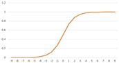 $f\left(x\right)={\displaystyle \frac{1}{1+e^{-x}}}$	Incremental, cross-validation and batch Incremental, cross-validation and batch	15/94/1	0.767	0.967	1. Operation and behavior: activation functions, training methods, hyperparameters 2. Neural model: multilayer perceptron 3. Activation functions: sigmoidea (sigmoid axon) 4. Training method: error backpropagation (RProp) 5. Loss function: incremental in the cross-validation set 6. Optimization algorithm: MSE (mean square error) 7. Epochs: 635 8. Weight initialization: batch
02	Collector efficiency factor				10/88/2	0.026	0.988
	Collector heat removal factor					0.028	0.988
03	Collector outlet fluid temperature				10/70/3	3.534	0.895
	Collector useful energy gain					73.855	0.966
	Global collector efficiency					2.176	0.994

Where: MAE stands for mean absolute error, r is the correlation coefficient, the nomenclature (9/95/2) highlights number of neurons in the input vector (9), hidden layer (95) and output layer (2), and BP-MLP stands for multilayer perceptron that uses the back-propagation learning algorithm.

Figure 4. ANN 01 architecture: The figure depicts the architecture (topology + behavior) of the first artificial neural network model.

Figure 4. ANN 01 architecture: The figure depicts the architecture (topology + behavior) of the first artificial neural network model.

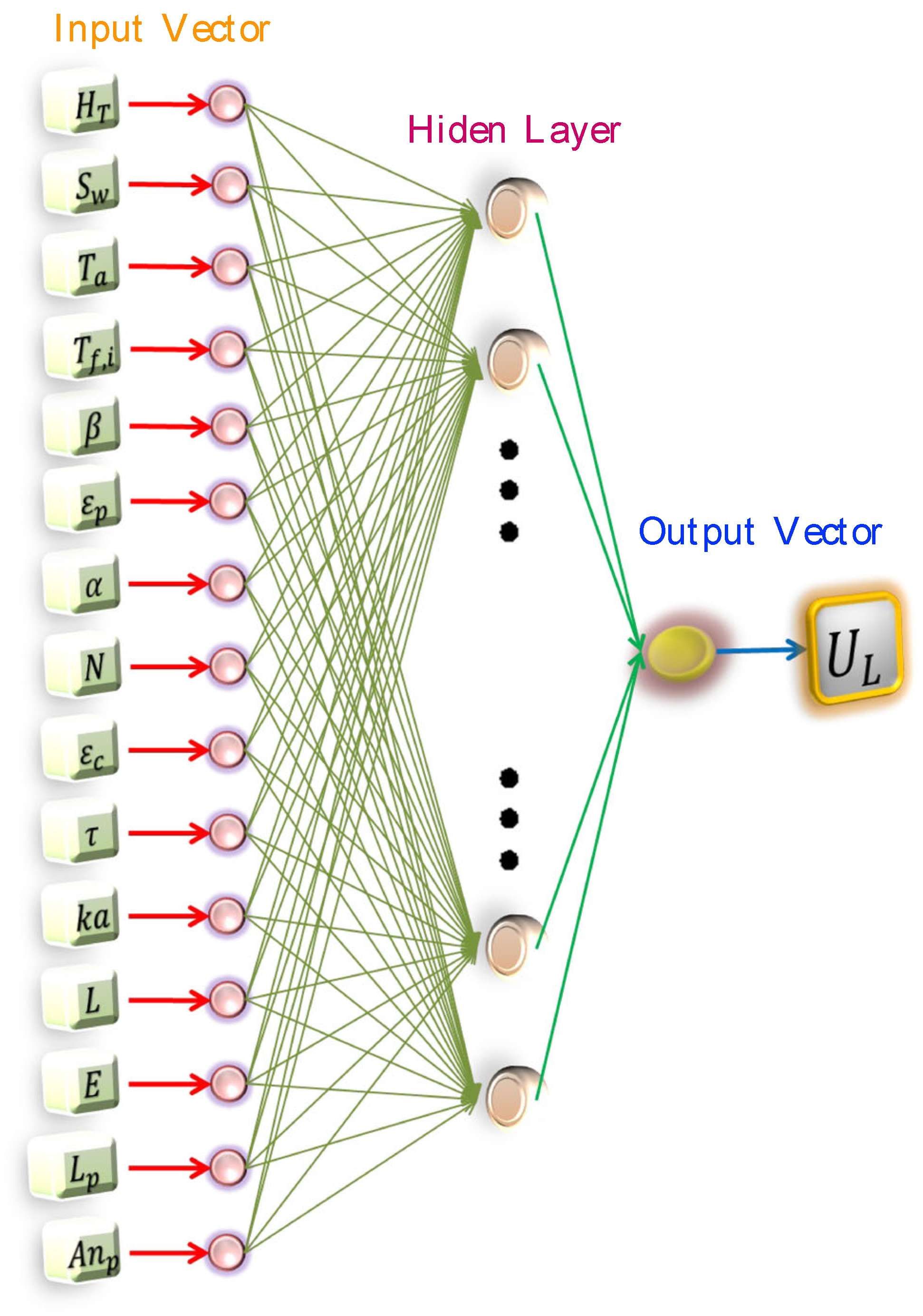
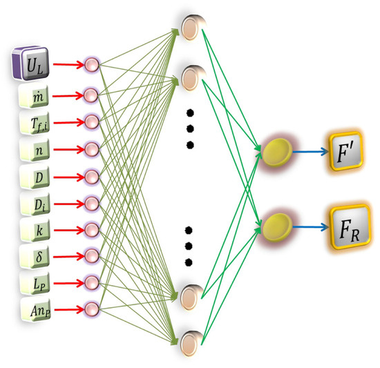
Figure 5. ANN 02 architecture: The figure depicts the architecture (topology + behavior) of the second Artificial Neural Network model.

Figure 5. ANN 02 architecture: The figure depicts the architecture (topology + behavior) of the second Artificial Neural Network model.

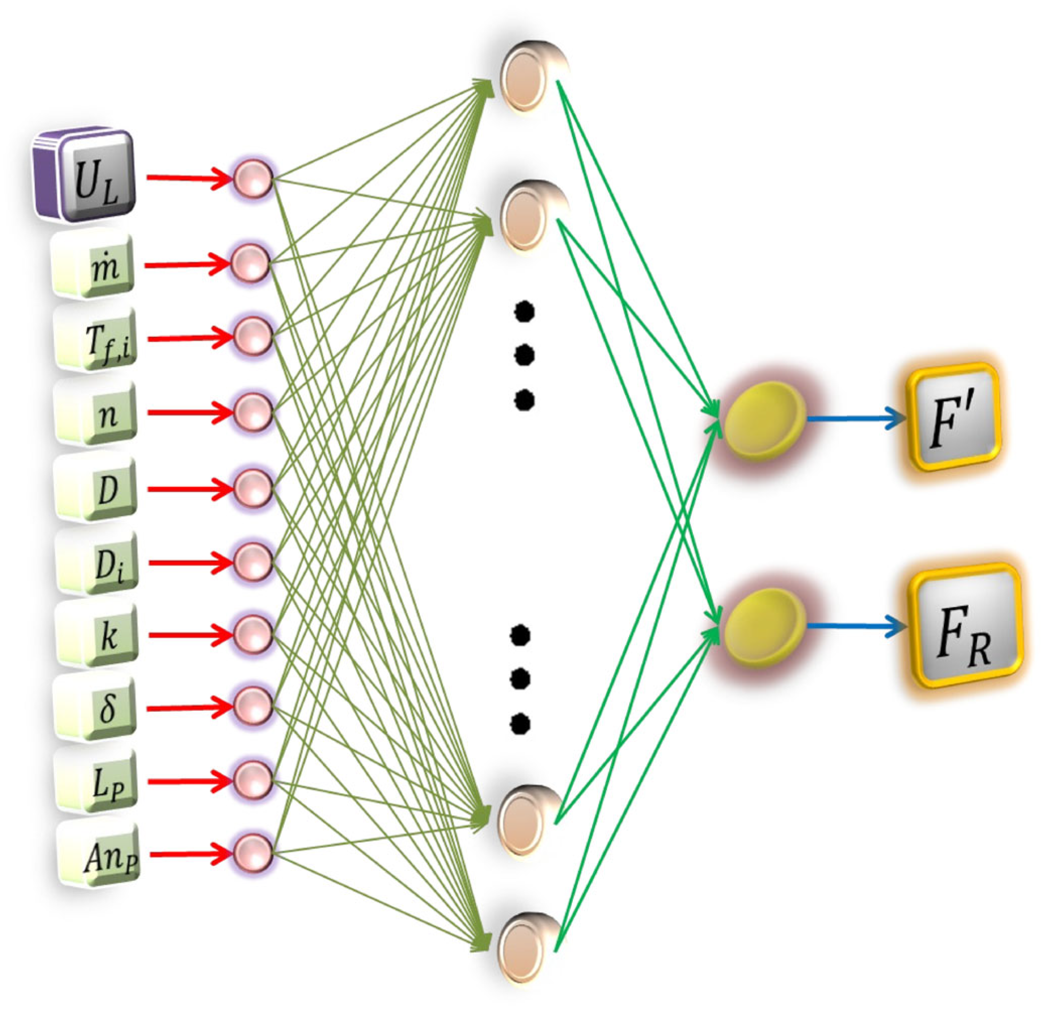
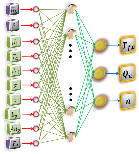
Figure 6. ANN 03 architecture: The figure depicts the architecture (topology + behavior) of the third artificial neural network model.

Figure 6. ANN 03 architecture: The figure depicts the architecture (topology + behavior) of the third artificial neural network model.

2.2.2. Part 02: Data Sets for Training, Validation, and Testing

The neural model was developed in the software NeuroSolution 7 and data were organized in training (60%), cross-validation (15%), and testing (25%) as shown in Table 8.

Table 8. Database partition.

Stages of Supervised Learning	Percentage (%)	Number of Vectors
Training	60	635
Cross-validation	15	158
Testing	25	265

Table 8. Database partition.

Stages of Supervised Learning	Percentage (%)	Number of Vectors
Training	60	635
Cross-validation	15	158
Testing	25	265

A stopping criterion was established at 635 iterations based on the mean squared error (MSE) to prevent overtraining of the neural network. The updating of data weights during the training phase was executed through the batch weight update method [33]. The data employed in the three proposed interconnected neural networks are detailed in Table 9, Table 10 and Table 11.

2.3. Validation of the PINNs Model against Experimental Data

To rigorously evaluate the proposed PINNs model, a validation study was performed by comparing its predictions with experimental data derived from a constructed flat-plate solar collector. The experimental data, originally analyzed by Alvarez et al. (2010) [34], were evaluated using traditional thermodynamic equations to determine efficiency factors and temperature parameters (Table 12).

However, differences between the data ranges used for training the artificial neural network and those from Alvarez et al. (2010) necessitated additional adjustments. Specifically, the ANN required further training to recalibrate its architecture to align with the new data ranges provided. The adjusted topology of the ANN model, reflecting these modifications, is detailed in Table 13. This refinement was essential for ensuring that the PINNs model accurately mirrored the experimental results and effectively addressed the performance metrics outlined in the traditional thermodynamic analyses.

Table 9. Data set to predict the collector overall loss coefficient.

Mapping	Indicator Excel Number	Global Solar Radiation (W/m2)	Wind Speed (m/s)	Ambient Temperature (°C)	Inlet Fluid Temperature (°C)	Collector Tilt (°Sex)	Plate Emittance (------)	Plate Absorptance (------)	Number of Covers (------)	Cover Emittance (------)	Cover Transmittane (------)	Insulation Thermal Conductivity (W/(m·K))	Lower Insulation Thickness (m)	Lateral Insulation Thickness (m)	Plate Length (m)	Plate Width (m)	Collector Overall Loss Coefficient (W/(m2·K))
Training	2	946	0.32	29.4	32.6	16.5	0.05	0.85	2	0.14	0.9	0.13	0.27	0.11	1	2.1	2.5911
	3	946	0.48	30	32.9	9.5	0.03	0.47	4	0.14	0.9	0.029	0.41	0.14	1.9	0.7	0.8532
	4	854	1.8	26	27	14.5	0.92	0.97	4	0.14	0.9	0.06	0.21	0.004	1.45	2.8	7.7695
	.	.	.	.	.	.	.	.	.	.	.	.	.	.	.	.	.
	.	.	.	.	.	.	.	.	.	.	.	.	.	.	.	.	.
	.	.	.	.	.	.	.	.	.	.	.	.	.	.	.	.	.
	634	946	0.48	30	32.9	28	0.75	0.89	1	0.87	0.84	0.19	0.45	0.13	1.5	0.3	9.9809
	635	944	0.38	29	32.6	10	0.14	0.89	1	0.04	0.88	0.032	0.33	0.01	0.25	2.1	11.8766
	636	946	0.48	30	32.9	8	0.87	0.95	4	0.69	0.92	0.13	0.26	0.032	0.3	1.7	10.0846
Cross-validation	637	942	0.44	27.1	29.9	13	0.87	0.95	1	0.98	0.82	0.33	0.35	0.085	1.25	0.6	12.4500
	638	576	0.4	22	21	8.5	0.9	0.94	1	0.19	0.91	0.35	0.32	0.14	2.1	1.0	6.5936
	639	946	0.32	29.4	32.6	27	0.82	0.08	1	0.14	0.9	0.029	0.18	0.004	1.45	1.8	5.3210
	.	.	.	.	.	.	.	.	.	.	.	.	.	.	.	.	.
	.	.	.	.	.	.	.	.	.	.	.	.	.	.	.	.	.
	.	.	.	.	.	.	.	.	.	.	.	.	.	.	.	.	.
	792	946	0.48	30	32.9	27	0.85	0.25	2	0.76	0.74	0.028	0.035	0.1	0.75	0.9	3.0152
	793	932	0.27	23.4	26.4	32	0.9	0.94	3	0.69	0.92	0.24	0.27	0.044	2.5	2.8	5.6508
	794	936	0.25	26.6	30	20	0.05	0.85	4	0.69	0.92	0.029	0.1	0.036	1.4	2.6	2.2576
Testing	795	923	0.05	19.2	24.7	13	0.85	0.25	3	0.87	0.84	0.029	0.25	0.13	1	5.5	2.3852
	796	939	0.42	25.5	26	8	0.85	0.25	1	0.69	0.92	0.33	0.17	0.08	5.5	0.9	7.6782
	797	932	0.17	24.8	28.8	18	0.75	0.89	3	0.53	0.73	0.06	0.04	0.01	2.9	0.6	3.8148
	.	.	.	.	.	.	.	.	.	.	.	.	.	.	.	.	.
	.	.	.	.	.	.	.	.	.	.	.	.	.	.	.	.	.
	.	.	.	.	.	.	.	.	.	.	.	.	.	.	.	.	.
	1057	946	0.48	30	32.9	8	0.9	0.26	2	0.98	0.82	0.046	0.17	0.004	1.25	0.9	10.7509
	1058	933	0.22	24.1	26.2	40	0.9	0.26	4	0.89	0.78	0.046	0.06	0.016	1.4	2.1	2.6093
	1059	936	0.23	24.6	27.5	23	0.87	0.13	4	0.19	0.91	0.19	0.38	0.012	6	5.5	5.3641

Table 9. Data set to predict the collector overall loss coefficient.

Mapping	Indicator Excel Number	Global Solar Radiation (W/m2)	Wind Speed (m/s)	Ambient Temperature (°C)	Inlet Fluid Temperature (°C)	Collector Tilt (°Sex)	Plate Emittance (------)	Plate Absorptance (------)	Number of Covers (------)	Cover Emittance (------)	Cover Transmittane (------)	Insulation Thermal Conductivity (W/(m·K))	Lower Insulation Thickness (m)	Lateral Insulation Thickness (m)	Plate Length (m)	Plate Width (m)	Collector Overall Loss Coefficient (W/(m2·K))
Training	2	946	0.32	29.4	32.6	16.5	0.05	0.85	2	0.14	0.9	0.13	0.27	0.11	1	2.1	2.5911
	3	946	0.48	30	32.9	9.5	0.03	0.47	4	0.14	0.9	0.029	0.41	0.14	1.9	0.7	0.8532
	4	854	1.8	26	27	14.5	0.92	0.97	4	0.14	0.9	0.06	0.21	0.004	1.45	2.8	7.7695
	.	.	.	.	.	.	.	.	.	.	.	.	.	.	.	.	.
	.	.	.	.	.	.	.	.	.	.	.	.	.	.	.	.	.
	.	.	.	.	.	.	.	.	.	.	.	.	.	.	.	.	.
	634	946	0.48	30	32.9	28	0.75	0.89	1	0.87	0.84	0.19	0.45	0.13	1.5	0.3	9.9809
	635	944	0.38	29	32.6	10	0.14	0.89	1	0.04	0.88	0.032	0.33	0.01	0.25	2.1	11.8766
	636	946	0.48	30	32.9	8	0.87	0.95	4	0.69	0.92	0.13	0.26	0.032	0.3	1.7	10.0846
Cross-validation	637	942	0.44	27.1	29.9	13	0.87	0.95	1	0.98	0.82	0.33	0.35	0.085	1.25	0.6	12.4500
	638	576	0.4	22	21	8.5	0.9	0.94	1	0.19	0.91	0.35	0.32	0.14	2.1	1.0	6.5936
	639	946	0.32	29.4	32.6	27	0.82	0.08	1	0.14	0.9	0.029	0.18	0.004	1.45	1.8	5.3210
	.	.	.	.	.	.	.	.	.	.	.	.	.	.	.	.	.
	.	.	.	.	.	.	.	.	.	.	.	.	.	.	.	.	.
	.	.	.	.	.	.	.	.	.	.	.	.	.	.	.	.	.
	792	946	0.48	30	32.9	27	0.85	0.25	2	0.76	0.74	0.028	0.035	0.1	0.75	0.9	3.0152
	793	932	0.27	23.4	26.4	32	0.9	0.94	3	0.69	0.92	0.24	0.27	0.044	2.5	2.8	5.6508
	794	936	0.25	26.6	30	20	0.05	0.85	4	0.69	0.92	0.029	0.1	0.036	1.4	2.6	2.2576
Testing	795	923	0.05	19.2	24.7	13	0.85	0.25	3	0.87	0.84	0.029	0.25	0.13	1	5.5	2.3852
	796	939	0.42	25.5	26	8	0.85	0.25	1	0.69	0.92	0.33	0.17	0.08	5.5	0.9	7.6782
	797	932	0.17	24.8	28.8	18	0.75	0.89	3	0.53	0.73	0.06	0.04	0.01	2.9	0.6	3.8148
	.	.	.	.	.	.	.	.	.	.	.	.	.	.	.	.	.
	.	.	.	.	.	.	.	.	.	.	.	.	.	.	.	.	.
	.	.	.	.	.	.	.	.	.	.	.	.	.	.	.	.	.
	1057	946	0.48	30	32.9	8	0.9	0.26	2	0.98	0.82	0.046	0.17	0.004	1.25	0.9	10.7509
	1058	933	0.22	24.1	26.2	40	0.9	0.26	4	0.89	0.78	0.046	0.06	0.016	1.4	2.1	2.6093
	1059	936	0.23	24.6	27.5	23	0.87	0.13	4	0.19	0.91	0.19	0.38	0.012	6	5.5	5.3641

Table 10. Data set to predict the collector efficiency factor and collector heat removal factor.

Mapping	Indicator Excel Number	Collector Overall Loss Coefficient (W/(m2·K))	Ambient Temperature (°C)	Mass Flow Rate (kg/s)	Number of Paralels Tubes (a.u.)	Outside Tube Diameter (mm)	Inside Tube Diameter (mm)	Plate Thermal Conductivity (W/(m·K))	Plate Thickness (mm)	Plate Length (m)	Plate Width (m)	Collector Efficiency Factor (a.u.)	Collector Heat Removal Factor (a.u.)
Training	2	2.59	32.6	0.36	19	22.23	18.92	19.5	3.7	1.00	2.1	0.9657	0.9640
	3	0.85	32.9	0.62	13	12.70	10.92	401.0	2.0	1.90	0.7	0.9995	0.9993
	4	7.77	27.0	0.02	3	9.53	8.00	429.0	1.1	1.45	2.8	0.3743	0.3411
	.	.	.	.	.	.	.	.	.	.	.	.	.
	.	.	.	.	.	.	.	.	.	.	.	.	.
	.	.	.	.	.	.	.	.	.	.	.	.	.
	634	9.98	32.9	0.38	2	28.58	26.04	15.0	5.6	1.50	0.3	0.8921	0.8910
	635	11.88	32.6	0.20	10	12.70	11.43	116.0	0.4	0.25	2.1	0.5591	0.5579
	636	10.08	32.9	0.24	10	15.88	14.45	73.0	1.4	0.30	1.7	0.8226	0.8209
Cross-validation	637	12.45	29.9	0.02	19	9.53	8.00	73.0	11.3	1.25	0.6	0.9516	0.8871
	638	6.59	21.0	0.01	3	28.58	26.80	80.0	2.8	2.10	1.0	0.6959	0.5634
	639	5.32	32.6	0.86	19	12.70	10.92	429.0	0.3	1.45	1.8	0.9755	0.9737
	.	.	.	.	.	.	.	.	.	.	.	.	.
	.	.	.	.	.	.	.	.	.	.	.	.	.
	.	.	.	.	.	.	.	.	.	.	.	.	.
	792	3.02	32.9	0.28	20	15.88	12.57	174.0	0.7	0.75	0.9	0.9907	0.9899
	793	5.65	26.4	0.03	3	28.58	26.04	80.0	0.4	2.50	2.8	0.1653	0.1603
	794	2.26	30.0	0.10	6	9.53	7.04	19.5	1.0	1.40	2.6	0.4385	0.4366
Testing	795	2.39	24.7	0.01	7	22.23	18.92	174.0	10.8	1.00	5.5	0.7729	0.6122
	796	7.68	26.0	0.02	8	12.70	10.92	174.0	4.4	5.50	0.9	0.8974	0.7446
	797	3.81	28.8	0.04	7	15.88	13.84	15.0	3.4	2.90	0.6	0.9422	0.9247
	.	.	.	.	.	.	.	.	.	.	.	.	.
	.	.	.	.	.	.	.	.	.	.	.	.	.
	.	.	.	.	.	.	.	.	.	.	.	.	.
	1057	10.75	32.9	0.70	14	15.88	14.45	51.0	5.6	1.25	0.9	0.9875	0.9856
	1058	2.61	26.2	0.02	17	15.88	13.84	51.0	3.0	1.40	2.1	0.9469	0.8941
	1059	5.36	27.5	0.02	9	22.23	18.92	317.0	8.5	6.00	5.5	0.6708	0.3006

Table 10. Data set to predict the collector efficiency factor and collector heat removal factor.

Mapping	Indicator Excel Number	Collector Overall Loss Coefficient (W/(m2·K))	Ambient Temperature (°C)	Mass Flow Rate (kg/s)	Number of Paralels Tubes (a.u.)	Outside Tube Diameter (mm)	Inside Tube Diameter (mm)	Plate Thermal Conductivity (W/(m·K))	Plate Thickness (mm)	Plate Length (m)	Plate Width (m)	Collector Efficiency Factor (a.u.)	Collector Heat Removal Factor (a.u.)
Training	2	2.59	32.6	0.36	19	22.23	18.92	19.5	3.7	1.00	2.1	0.9657	0.9640
	3	0.85	32.9	0.62	13	12.70	10.92	401.0	2.0	1.90	0.7	0.9995	0.9993
	4	7.77	27.0	0.02	3	9.53	8.00	429.0	1.1	1.45	2.8	0.3743	0.3411
	.	.	.	.	.	.	.	.	.	.	.	.	.
	.	.	.	.	.	.	.	.	.	.	.	.	.
	.	.	.	.	.	.	.	.	.	.	.	.	.
	634	9.98	32.9	0.38	2	28.58	26.04	15.0	5.6	1.50	0.3	0.8921	0.8910
	635	11.88	32.6	0.20	10	12.70	11.43	116.0	0.4	0.25	2.1	0.5591	0.5579
	636	10.08	32.9	0.24	10	15.88	14.45	73.0	1.4	0.30	1.7	0.8226	0.8209
Cross-validation	637	12.45	29.9	0.02	19	9.53	8.00	73.0	11.3	1.25	0.6	0.9516	0.8871
	638	6.59	21.0	0.01	3	28.58	26.80	80.0	2.8	2.10	1.0	0.6959	0.5634
	639	5.32	32.6	0.86	19	12.70	10.92	429.0	0.3	1.45	1.8	0.9755	0.9737
	.	.	.	.	.	.	.	.	.	.	.	.	.
	.	.	.	.	.	.	.	.	.	.	.	.	.
	.	.	.	.	.	.	.	.	.	.	.	.	.
	792	3.02	32.9	0.28	20	15.88	12.57	174.0	0.7	0.75	0.9	0.9907	0.9899
	793	5.65	26.4	0.03	3	28.58	26.04	80.0	0.4	2.50	2.8	0.1653	0.1603
	794	2.26	30.0	0.10	6	9.53	7.04	19.5	1.0	1.40	2.6	0.4385	0.4366
Testing	795	2.39	24.7	0.01	7	22.23	18.92	174.0	10.8	1.00	5.5	0.7729	0.6122
	796	7.68	26.0	0.02	8	12.70	10.92	174.0	4.4	5.50	0.9	0.8974	0.7446
	797	3.81	28.8	0.04	7	15.88	13.84	15.0	3.4	2.90	0.6	0.9422	0.9247
	.	.	.	.	.	.	.	.	.	.	.	.	.
	.	.	.	.	.	.	.	.	.	.	.	.	.
	.	.	.	.	.	.	.	.	.	.	.	.	.
	1057	10.75	32.9	0.70	14	15.88	14.45	51.0	5.6	1.25	0.9	0.9875	0.9856
	1058	2.61	26.2	0.02	17	15.88	13.84	51.0	3.0	1.40	2.1	0.9469	0.8941
	1059	5.36	27.5	0.02	9	22.23	18.92	317.0	8.5	6.00	5.5	0.6708	0.3006

Table 11. Data set to predict the outlet fluid temperature, collector useful energy gain and global collector efficiency.

Mapping	Indicator Excel Number	Collector Overall Loss Coefficient (W/(m2·K))	Collector Efficiency Factor (------)	Collector Heat Removal Factor (------)	Global Solar Radiation (W/m2)	Ambient Temperature (°C)	Inlet Fluid Temperature (°C)	Plate Absorptance (------)	Cover Transmittance (------)	Plate Length (m)	Plate Width (m)	Outlet Fluid Temperature (°C)	Collector Useful Energy Gain (W)	Global Collector Efficiency (%)
Training	2	2.5911	0.9657	0.9640	946	29.4	32.6	0.85	0.90	1.00	2.1	33.5738	1462.9330	73.6400
	3	0.8532	0.9995	0.9993	946	30.0	32.9	0.47	0.90	1.90	0.7	33.0915	495.7288	42.4313
	4	7.7695	0.3743	0.3411	854	26.0	27.0	0.97	0.90	1.45	2.8	43.9985	1032.0085	29.7646
	.	.	.	.	.	.	.	.	.	.	.	.	.	.
	.	.	.	.	.	.	.	.	.	.	.	.	.	.
	.	.	.	.	.	.	.	.	.	.	.	.	.	.
	634	9.9809	0.8921	0.8910	946	30.0	32.9	0.89	0.84	1.50	0.3	33.0733	274.7939	64.5511
	635	11.8766	0.5591	0.5579	944	29.0	32.6	0.89	0.88	0.25	2.1	32.8471	206.2085	41.6078
	636	10.0846	0.8226	0.8209	946	30.0	32.9	0.95	0.92	0.30	1.7	33.2369	337.3635	69.9257
Cross-validation	637	12.4500	0.9516	0.8871	942	27.1	29.9	0.95	0.82	1.25	0.6	37.5809	469.9361	66.5161
	638	6.5936	0.6959	0.5634	576	22.0	21.0	0.94	0.91	2.10	1.0	50.1297	566.7194	49.3177
	639	5.3210	0.9755	0.9737	946	29.4	32.6	0.08	0.90	1.45	1.8	32.6367	131.5501	5.3279
	.	.	.	.	.	.	.	.	.	.	.	.	.	.
	.	.	.	.	.	.	.	.	.	.	.	.	.	.
	.	.	.	.	.	.	.	.	.	.	.	.	.	.
	792	3.0152	0.9907	0.9899	946	30.0	32.9	0.25	0.74	0.75	0.9	32.9960	112.2647	17.5812
	793	5.6508	0.1653	0.1603	932	23.4	26.4	0.94	0.92	2.50	2.8	35.0532	894.1553	13.7056
	794	2.2576	0.4385	0.4366	936	26.6	30.0	0.85	0.92	1.40	2.6	32.7880	1162.6495	34.1249
Testing	795	2.3852	0.7729	0.6122	923	19.2	24.7	0.25	0.84	1.00	5.5	56.5427	614.9603	12.1139
	796	7.6782	0.8974	0.7446	939	25.5	26.0	0.25	0.92	5.50	0.9	35.5035	745.9813	16.9934
	797	3.8148	0.9422	0.9247	932	24.8	28.8	0.89	0.73	2.90	0.6	34.5799	959.5033	59.1672
	.	.	.	.	.	.	.	.	.	.	.	.	.	.
	.	.	.	.	.	.	.	.	.	.	.	.	.	.
	.	.	.	.	.	.	.	.	.	.	.	.	.	.
	1057	10.7509	0.9875	0.9856	946	30.0	32.9	0.26	0.82	1.25	0.9	32.9619	180.6728	17.9752
	1058	2.6093	0.9469	0.8941	933	24.1	26.2	0.26	0.78	1.40	2.1	34.1388	487.9389	17.7884
	1059	5.3641	0.6708	0.3006	936	24.6	27.5	0.13	0.91	6.00	5.5	47.3110	955.1287	3.0922

Table 11. Data set to predict the outlet fluid temperature, collector useful energy gain and global collector efficiency.

Mapping	Indicator Excel Number	Collector Overall Loss Coefficient (W/(m2·K))	Collector Efficiency Factor (------)	Collector Heat Removal Factor (------)	Global Solar Radiation (W/m2)	Ambient Temperature (°C)	Inlet Fluid Temperature (°C)	Plate Absorptance (------)	Cover Transmittance (------)	Plate Length (m)	Plate Width (m)	Outlet Fluid Temperature (°C)	Collector Useful Energy Gain (W)	Global Collector Efficiency (%)
Training	2	2.5911	0.9657	0.9640	946	29.4	32.6	0.85	0.90	1.00	2.1	33.5738	1462.9330	73.6400
	3	0.8532	0.9995	0.9993	946	30.0	32.9	0.47	0.90	1.90	0.7	33.0915	495.7288	42.4313
	4	7.7695	0.3743	0.3411	854	26.0	27.0	0.97	0.90	1.45	2.8	43.9985	1032.0085	29.7646
	.	.	.	.	.	.	.	.	.	.	.	.	.	.
	.	.	.	.	.	.	.	.	.	.	.	.	.	.
	.	.	.	.	.	.	.	.	.	.	.	.	.	.
	634	9.9809	0.8921	0.8910	946	30.0	32.9	0.89	0.84	1.50	0.3	33.0733	274.7939	64.5511
	635	11.8766	0.5591	0.5579	944	29.0	32.6	0.89	0.88	0.25	2.1	32.8471	206.2085	41.6078
	636	10.0846	0.8226	0.8209	946	30.0	32.9	0.95	0.92	0.30	1.7	33.2369	337.3635	69.9257
Cross-validation	637	12.4500	0.9516	0.8871	942	27.1	29.9	0.95	0.82	1.25	0.6	37.5809	469.9361	66.5161
	638	6.5936	0.6959	0.5634	576	22.0	21.0	0.94	0.91	2.10	1.0	50.1297	566.7194	49.3177
	639	5.3210	0.9755	0.9737	946	29.4	32.6	0.08	0.90	1.45	1.8	32.6367	131.5501	5.3279
	.	.	.	.	.	.	.	.	.	.	.	.	.	.
	.	.	.	.	.	.	.	.	.	.	.	.	.	.
	.	.	.	.	.	.	.	.	.	.	.	.	.	.
	792	3.0152	0.9907	0.9899	946	30.0	32.9	0.25	0.74	0.75	0.9	32.9960	112.2647	17.5812
	793	5.6508	0.1653	0.1603	932	23.4	26.4	0.94	0.92	2.50	2.8	35.0532	894.1553	13.7056
	794	2.2576	0.4385	0.4366	936	26.6	30.0	0.85	0.92	1.40	2.6	32.7880	1162.6495	34.1249
Testing	795	2.3852	0.7729	0.6122	923	19.2	24.7	0.25	0.84	1.00	5.5	56.5427	614.9603	12.1139
	796	7.6782	0.8974	0.7446	939	25.5	26.0	0.25	0.92	5.50	0.9	35.5035	745.9813	16.9934
	797	3.8148	0.9422	0.9247	932	24.8	28.8	0.89	0.73	2.90	0.6	34.5799	959.5033	59.1672
	.	.	.	.	.	.	.	.	.	.	.	.	.	.
	.	.	.	.	.	.	.	.	.	.	.	.	.	.
	.	.	.	.	.	.	.	.	.	.	.	.	.	.
	1057	10.7509	0.9875	0.9856	946	30.0	32.9	0.26	0.82	1.25	0.9	32.9619	180.6728	17.9752
	1058	2.6093	0.9469	0.8941	933	24.1	26.2	0.26	0.78	1.40	2.1	34.1388	487.9389	17.7884
	1059	5.3641	0.6708	0.3006	936	24.6	27.5	0.13	0.91	6.00	5.5	47.3110	955.1287	3.0922

Table 12. Design conditions for a constructed solar collector [34].

Experimental Data	Magnitude
Ambient temperature (°C)	20
Collector heat removal factor	765
Collector tilt (°Sexa.)	60
Cover emittance (a.u.)	0.9
Cover transmittance (a.u.)	0.82
Global solar irradiation (W/m2)	1088
Inlet fluid temperature (°C)	15
Inside tube diameter (mm)	9
Insulation thermal conductivity (W/(m·K))	0.07
Lateral insulation thickness (mm)	10
Lower insulation thickness (mm)	30
Mass flow rate (kg/s)	0.01
Number of covers (a.u.)	1
Number of parallels tubes (units)	11
Outside tube diameter (mm)	10
Plate absorptance (a.u.)	0.9
Plate emittance (a.u.)	0.9
Plate length (m)	2
Plate thermal conductivity (W/(m·K))	385
Plate thickness (mm)	0.5
Plate width (m)	1
Wind speed (m/s)	0.4

Table 12. Design conditions for a constructed solar collector [34].

Experimental Data	Magnitude
Ambient temperature (°C)	20
Collector heat removal factor	765
Collector tilt (°Sexa.)	60
Cover emittance (a.u.)	0.9
Cover transmittance (a.u.)	0.82
Global solar irradiation (W/m2)	1088
Inlet fluid temperature (°C)	15
Inside tube diameter (mm)	9
Insulation thermal conductivity (W/(m·K))	0.07
Lateral insulation thickness (mm)	10
Lower insulation thickness (mm)	30
Mass flow rate (kg/s)	0.01
Number of covers (a.u.)	1
Number of parallels tubes (units)	11
Outside tube diameter (mm)	10
Plate absorptance (a.u.)	0.9
Plate emittance (a.u.)	0.9
Plate length (m)	2
Plate thermal conductivity (W/(m·K))	385
Plate thickness (mm)	0.5
Plate width (m)	1
Wind speed (m/s)	0.4

Table 13. ANN validation model and topology.

ANN Case	Output	ANN Model	Activation Function	Training	Topology	MAE	R	Connections
01	Collector overall loss coefficient	BP-MLP	Sigmoid function $f\left(x\right)={\displaystyle \frac{1}{1+e^{-x}}}$	Incremental, cross-validation and batch Incremental, cross-validation and batch	15/70/1	0.611	0.980	1. Operation and behavior: activation functions, training methods, hyperparameters 2. Neural model: multilayer perceptron 3. Activation functions: sigmoid (sigmoidaxon) 4. Training method: error backpropagation (RProp) 5. Loss function: incremental in the cross-validation set 6. Optimization algorithm: mean square error (MSE) 7. Epochs: 635 8. Weight initialization: batch
02	Collector efficiency factor				10/60/2	0.060	0.945
	Collector heat removal factor					0.079	0.923
03	Collector outlet fluid temperature				10/70/3	3.816	0.859
	Collector useful energy gain					68.414	0.972
	Global collector efficiency					2.194	0.994

Table 13. ANN validation model and topology.

ANN Case	Output	ANN Model	Activation Function	Training	Topology	MAE	R	Connections
01	Collector overall loss coefficient	BP-MLP	Sigmoid function $f\left(x\right)={\displaystyle \frac{1}{1+e^{-x}}}$	Incremental, cross-validation and batch Incremental, cross-validation and batch	15/70/1	0.611	0.980	1. Operation and behavior: activation functions, training methods, hyperparameters 2. Neural model: multilayer perceptron 3. Activation functions: sigmoid (sigmoidaxon) 4. Training method: error backpropagation (RProp) 5. Loss function: incremental in the cross-validation set 6. Optimization algorithm: mean square error (MSE) 7. Epochs: 635 8. Weight initialization: batch
02	Collector efficiency factor				10/60/2	0.060	0.945
	Collector heat removal factor					0.079	0.923
03	Collector outlet fluid temperature				10/70/3	3.816	0.859
	Collector useful energy gain					68.414	0.972
	Global collector efficiency					2.194	0.994

2.4. Case Study: Residencial House—Family Demand

For the design of the flat-plate collector, detailed in Table 14, the system was tailored to meet the annual thermal energy demand of a single-family residence located in Riobamba, central Ecuador, over the Andes. The design process utilized the above neural models, accounting for the requisite surface area for energy capture to be greater than that demanded.

Key environmental parameters that factored into the design include global solar radiation, wind speed, ambient temperature, inlet fluid temperature, mass flow rate, and collector tilt, all specific to the local climatic conditions. Additionally, the material thermal properties and collector geometry were meticulously defined as input variables for the neural models. These parameters include the number of tubes, outside and inside tube diameters, plate emittance, plate absorptance, plate thermal conductivity, plate thickness, number of covers, cover emittance, cover transmittance, insulation thickness (both lower and lateral), and dimensions of the plate such as length and width.

Table 14. Design conditions for a solar collector in Ecuador.

Study Case	Units	Magnitude	Materials
Ambient temperature $T_a$	°C	12.75	a.u.
Collector tilt $\beta$	°Sexag.	8	a.u.
Cover emittance ${\epsilon }_c$	a.u.	0.9	Greenhouse rigid plastic (PVC wavy)
Cover transmittance $\tau$	a.u.	0.82	Greenhouse rigid plastic (PVC wavy)
Demanded thermal power $Dpd$	W	726.7	a.u.
Global solar radiation $H_T$	W/m2	742	a.u.
Inlet fluid temperature $T_{fi}$	°C	13.2	Water
Inside tube diameter $D_i$	mm	8.001	Galvanized tube, type L
Insulation thermal conductivity $ka$	W/(m·K)	0.06	Shells of pressed wheat (90 kg/m3)
Lateral insulation thickness $E$	mm	25	Shells of pressed wheat (90 kg/m3)
Lower insulation thickness $L$	mm	50	Shells of pressed wheat (90 kg/m3)
Mass flow rate $\dot{m }$	kg/s	0.00371	Water
Number of covers N	a.u.	1	Greenhouse rigid plastic (PVC wavy)
Number of parallels tubes N	a.u.	12	Galvanized tube, type L
Outside tube diameter $D$	Mm	9.525	Galvanized tube, type L
Plate absorptance $\alpha$	a.u.	0.7	(Electrostatic black paint)
Plate effective area $Ae$	m2	2.8	a.u.
Plate emittance ${\epsilon }_p$	a.u.	0.2	Selective surface of galvanized steel
Plate length $L_p$	m	2.25	Galvanized plate
Plate thermal conductivity $k$	W/(m·K)	58	Galvanized plate
Plate thickness $\delta$	Mm	2	(Electrostatic black paint)
Plate width $A{n}_P$	m	1.25	Galvanized plate
Wind speed $S_w$	m/s	2.19	a.u.

Table 14. Design conditions for a solar collector in Ecuador.

Study Case	Units	Magnitude	Materials
Ambient temperature $T_a$	°C	12.75	a.u.
Collector tilt $\beta$	°Sexag.	8	a.u.
Cover emittance ${\epsilon }_c$	a.u.	0.9	Greenhouse rigid plastic (PVC wavy)
Cover transmittance $\tau$	a.u.	0.82	Greenhouse rigid plastic (PVC wavy)
Demanded thermal power $Dpd$	W	726.7	a.u.
Global solar radiation $H_T$	W/m2	742	a.u.
Inlet fluid temperature $T_{fi}$	°C	13.2	Water
Inside tube diameter $D_i$	mm	8.001	Galvanized tube, type L
Insulation thermal conductivity $ka$	W/(m·K)	0.06	Shells of pressed wheat (90 kg/m3)
Lateral insulation thickness $E$	mm	25	Shells of pressed wheat (90 kg/m3)
Lower insulation thickness $L$	mm	50	Shells of pressed wheat (90 kg/m3)
Mass flow rate $\dot{m }$	kg/s	0.00371	Water
Number of covers N	a.u.	1	Greenhouse rigid plastic (PVC wavy)
Number of parallels tubes N	a.u.	12	Galvanized tube, type L
Outside tube diameter $D$	Mm	9.525	Galvanized tube, type L
Plate absorptance $\alpha$	a.u.	0.7	(Electrostatic black paint)
Plate effective area $Ae$	m2	2.8	a.u.
Plate emittance ${\epsilon }_p$	a.u.	0.2	Selective surface of galvanized steel
Plate length $L_p$	m	2.25	Galvanized plate
Plate thermal conductivity $k$	W/(m·K)	58	Galvanized plate
Plate thickness $\delta$	Mm	2	(Electrostatic black paint)
Plate width $A{n}_P$	m	1.25	Galvanized plate
Wind speed $S_w$	m/s	2.19	a.u.

3. Results

3.1. ANN Predictive Capability

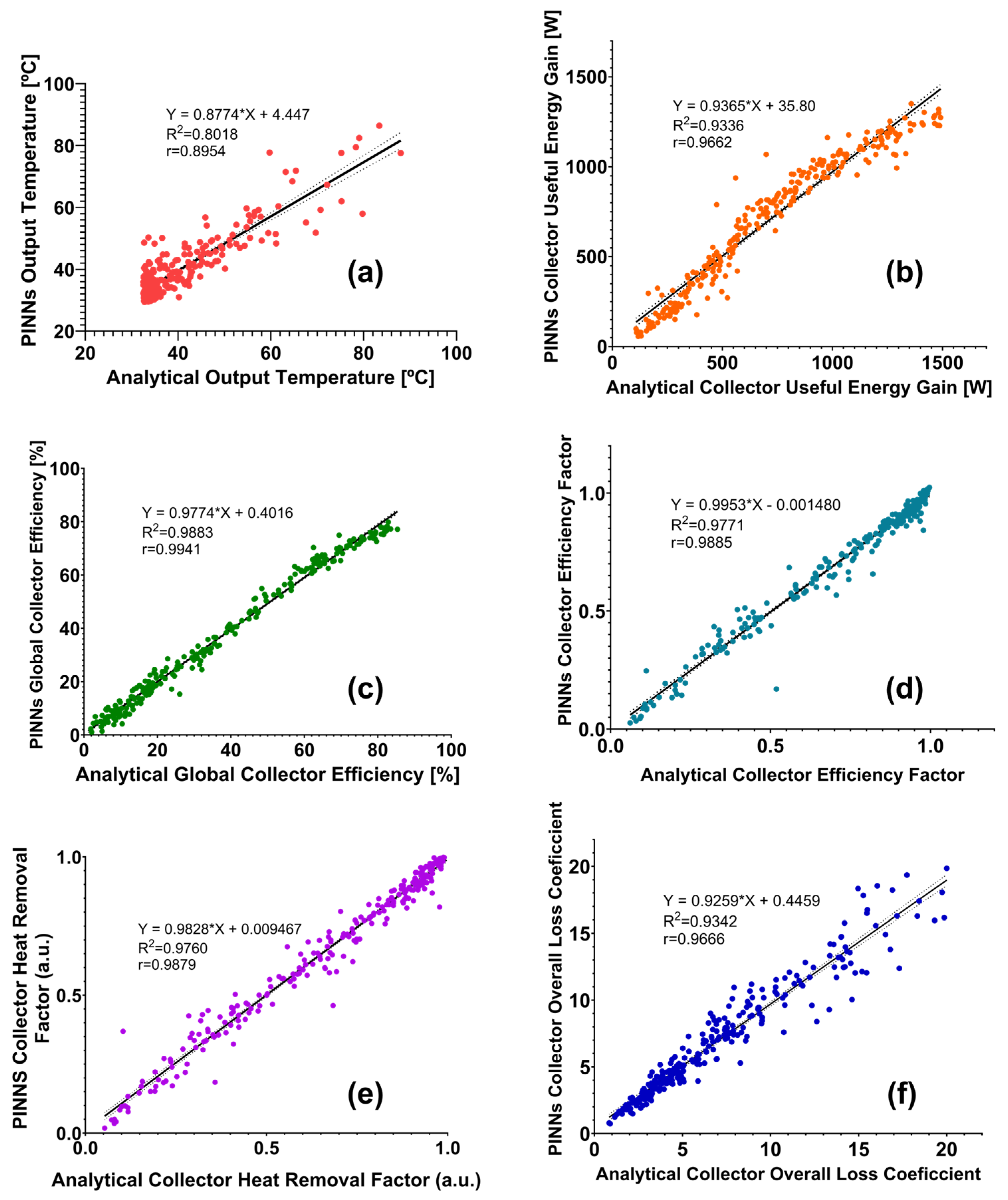
The comparative analysis between analytical models and physics-informed neural networks for solar collector design reveals compelling insights into the efficacy of PINNs as a modeling approach. Six key parameters were examined: output temperature, collector useful energy gain, global collector efficiency, collector heat removal factor, collector overall loss coefficient, and collector efficiency factor. The results indicate that while the PINNs and simplified thermodynamic equations produce similar outcomes for key parameters, the PINNs excel in capturing complex nonlinear behaviors that traditional methods cannot easily quantify. This provides a more comprehensive modeling approach where conventional engineering design equations may fall short.

3.1.1. Output Temperature Analysis

The relationship between analytical and PINNs output temperatures (Figure 7a) is described by the equation Y = 0.8774X + 4.447, where Y represents the PINNs output and X the analytical output. The coefficient of determination (R² = 0.8018) indicates that approximately 80.18% of the variance in the PINNs output is explained by the analytical model. While this represents the lowest R² value among the parameters studied, it still signifies a strong correlation. The Pearson correlation coefficient (r = 0.8954) further supports this, suggesting a robust positive correlation between the two methods. The slope of less than 1 (0.8774) implies that the PINNs model computes a slightly different output temperature compared to the analytical model, particularly at higher temperatures. This minor discrepancy could be attributed to the complex, non-linear nature of heat transfer processes in solar collectors, which may be more challenging for the conventional approach.

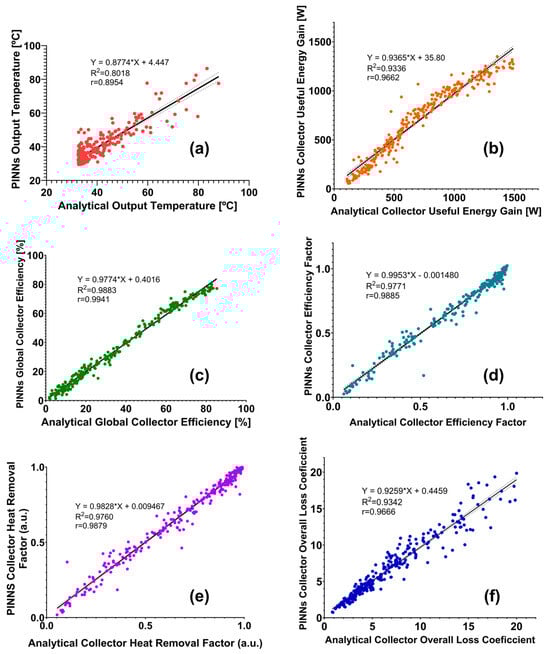
Figure 7. Correlations between ANN outputs and expected values (a) output temperature, (b) collector useful energy gain, (c) global collector efficiency, (d) collector efficiency factor, (e) collector heat removal factor, and (f) collector overall loss coefficient.

Figure 7. Correlations between ANN outputs and expected values (a) output temperature, (b) collector useful energy gain, (c) global collector efficiency, (d) collector efficiency factor, (e) collector heat removal factor, and (f) collector overall loss coefficient.

3.1.2. Collector Useful Energy Gain

For the collector useful energy gain, the relationship is expressed as Y = 0.9365X + 35.80. The higher R² value of 0.9336 indicates that 93.36% of the variance in the PINNs results is accounted for by the analytical model, representing a significant improvement over the temperature prediction (Figure 7b). The Pearson correlation coefficient (r = 0.9662) demonstrates a very strong positive correlation between the two approaches. The slope closer to 1 (0.9365) suggests that the PINNs model more accurately predicts the useful energy gain across the range of values, with a slight overestimation at lower values due to the positive intercept (35.80).

3.1.3. Global Collector Efficiency

The global collector efficiency (Figure 7c) shows exceptional agreement between the two methods, with a relationship of Y = 0.9774X + 0.4016. The remarkably high R² value (0.9883) suggests that 98.83% of the variance in the PINNs results is explained by the analytical model. The Pearson correlation coefficient (r = 0.9941) indicates an almost perfect positive correlation. This outstanding agreement implies that the PINNs model is particularly adept at capturing the overall performance characteristics of the solar collector, which is crucial for system-level design and optimization.

3.1.4. Collector Heat Removal Factor

The collector heat removal factor (Figure 7d) relationship is described by Y = 0.9828X + 0.009467. The R² value of 0.9760 shows that 97.60% of the variance in the PINNs results is accounted for by the analytical model. The high Pearson correlation coefficient (r = 0.9879) again indicates a very strong positive correlation. The slope very close to 1 (0.9828) and the near-zero intercept (0.009467) suggest that the PINNs model accurately predicts this parameter across the entire range of values, with only minimal deviation from the analytical model.

3.1.5. Collector Overall Loss Coefficient

For the collector overall loss coefficient (Figure 7e), the relationship is Y = 0.9259X + 0.4459. The R² value of 0.9342 suggests that 93.42% of the variance in the PINNs results is explained by the analytical model. The Pearson correlation coefficient (r = 0.9666) shows a very strong positive correlation between the two methods. The slope of 0.9259 indicates a slight underestimation by the PINNs model, particularly at higher loss coefficient values. This minor discrepancy could be due to the complex interplay of various heat loss mechanisms, which may require further refinement in the PINNs model to capture fully.

3.1.6. Collector Efficiency Factor

The collector efficiency factor (Figure 7f) demonstrates excellent agreement, with a relationship of Y = 0.9953X − 0.001480. The high R² value (0.9771) indicates that 97.71% of the variance in the PINNs results is accounted for by the analytical model. The Pearson correlation coefficient (r = 0.9885) demonstrates a very strong positive correlation. Notably, the slope is very close to 1 (0.9953) with a near-zero intercept (−0.001480), indicating that the PINNs model predicts this parameter with high accuracy across the entire range of values.

3.2. Validation of the ANN Model against Experimental Data

The comparative analysis between PINNs and analytical models for solar collector parameters reveals a nuanced picture of predictive accuracy and model performance. The output temperature prediction (Figure 8a) presents the most significant deviation, with a moderate correlation (R² = 0.736) and substantial underestimation by PINNs at higher temperatures (slope = 0.7806). This discrepancy highlights the challenges in modeling the complex, non-linear thermal behavior of solar collectors, particularly under high-temperature conditions. The collector useful energy gain (Figure 8b) shows a moderate positive correlation (R² = 0.8150), with PINNs underestimating at higher values (slope = 0.7639). Notably, the global collector efficiency (Figure 8c) exhibits the strongest correlation (R² = 0.9672), with near-perfect agreement between PINNs and analytical models (slope = 0.9521). This robust performance in predicting overall efficiency is particularly encouraging, as it represents a critical parameter for practical solar collector applications.

Figure 8. Correlations between ANN outputs and expected values (a) output temperature, (b) collector useful energy gain, (c) global collector efficiency, (d) collector efficiency factor, (e) collector heat removal factor, and (f) collector overall loss coefficient. The data point highlighted with dashed lines represents the comparison between the factors calculated using the thermodynamic equations from the experimental model and the corresponding values predicted by the PINNs model. This comparison provides a clear visualization of the alignment between the experimental results and the model’s predictions, underscoring the accuracy and reliability of the PINNs-based approach.

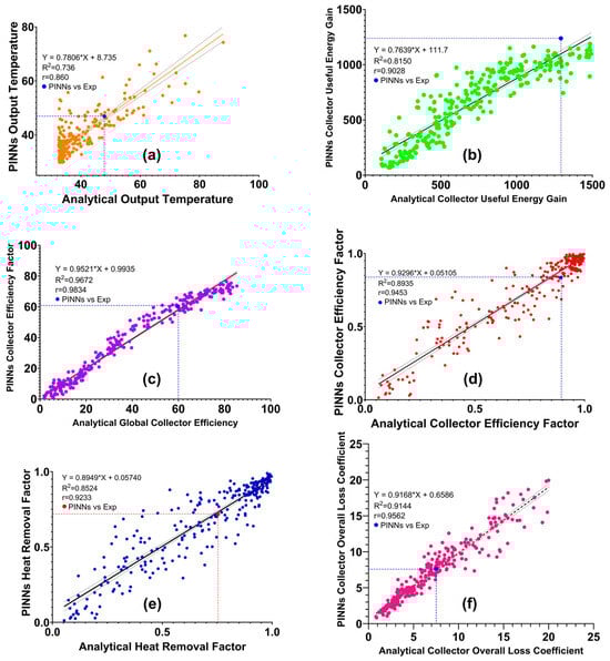
Figure 8. Correlations between ANN outputs and expected values (a) output temperature, (b) collector useful energy gain, (c) global collector efficiency, (d) collector efficiency factor, (e) collector heat removal factor, and (f) collector overall loss coefficient. The data point highlighted with dashed lines represents the comparison between the factors calculated using the thermodynamic equations from the experimental model and the corresponding values predicted by the PINNs model. This comparison provides a clear visualization of the alignment between the experimental results and the model’s predictions, underscoring the accuracy and reliability of the PINNs-based approach.

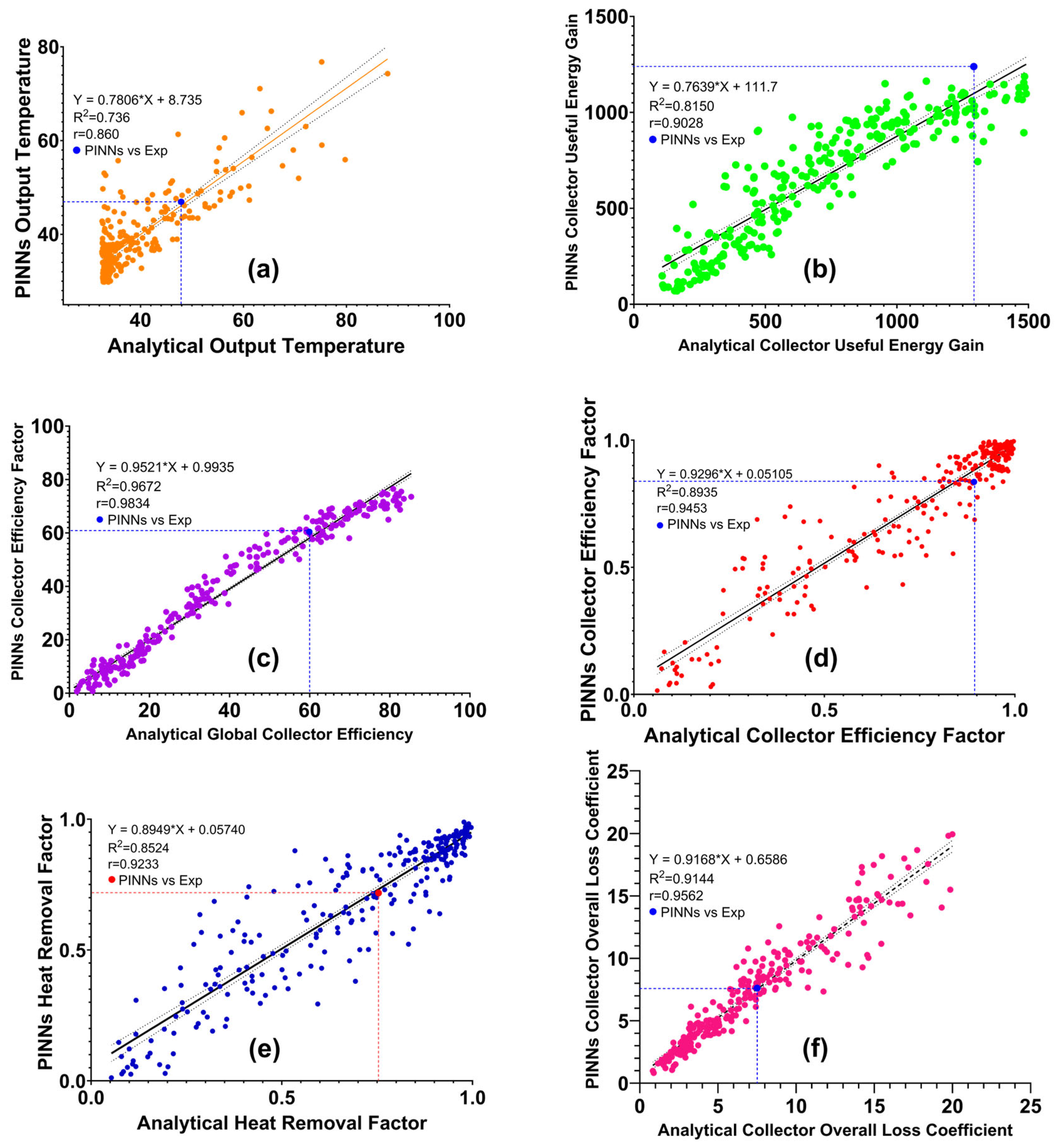
The collector efficiency factor and heat removal factor (Figure 8d,e) demonstrate strong positive correlations between PINNs and analytical models (R² = 0.8935 and 0.8524, respectively). The slight overestimation by PINNs in both cases (slopes of 0.9296 and 0.8949) suggests a systematic bias that, while minor, warrants further investigation. These results indicate that PINNs effectively capture the fundamental efficiency characteristics of solar collectors. The collector overall loss coefficient (Figure 8f) also shows strong agreement (R² = 0.9144, slope = 0.9168), indicating that PINNs accurately capture the thermal loss mechanisms within solar collectors. This ability to model heat loss is crucial for predicting long-term performance and optimizing collector designs.

Importantly, the comparison with experimental data from Alvarez et al. (2010) [34], represented by distinct points in each plot, reveals close agreement between PINNs predictions and real-world measurements for most parameters (Figure 8). The notable exception is the output temperature, where the deviation between PINNs and experimental data is more pronounced. This observation suggests that PINNs may be capturing subtle, non-linear aspects of solar collector behavior that are not fully accounted for in traditional analytical models. The ability of PINNs to potentially model these complex relationships, which are challenging for deterministic thermodynamic equations, represents a significant advantage of this approach.

3.3. Performance of the ANN in a Residential House Located in the Andes of Ecuador

Table 15 presents a comparative analysis of the design and performance of a solar collector using both a mathematical model and artificial neural networks for a residential house in the Andes of Ecuador. The inputs include key environmental and design parameters such as global solar radiation, wind speed, ambient temperature, inlet fluid temperature, mass flow rate, and collector geometry. The materials used in the collector, including galvanized tubes and plates with selective surfaces, are specified alongside these inputs.

The results for the thermodynamic model and ANN outputs reveal close agreement between the two approaches. The collector overall loss coefficient shows only a slight difference, with the ANN predicting 5.199 W/(m²·K) compared to 5.189 W/(m²·K) from the thermodynamic model. The collector efficiency factor and collector heat removal factor exhibit minor deviations, with the ANN results slightly underestimating F′ and overestimating F_R.

The collector outlet fluid temperature shows a more significant variation, with the ANN predicting a lower temperature of 55.05 °C compared to 67.22 °C from the thermodynamic model. Despite this difference, the predictions for collector useful energy gain and global collector efficiency are relatively close, with the ANN outputting 722.85 W and 33.68%, respectively, compared to 733.4 W and 35.15% from the thermodynamic model.

Table 15. Comparison between the outcomes of the mathematical and thermodynamics informer ANN models.

	Study Case	Abbreviation	Units	Results Thermodynamics Model	Results ANN
Output	Collector overall loss coefficient	$U_L$	W/(m2·K)	5.189	5.199
	Collector efficiency factor	$F^{\prime }$	a.u.	0.907	0.883
	Collector heat removal factor	$F_R$	a.u.	0.610	0.662
	Collector outlet fluid temperature	$T_{fo}$	°C	67.22	55.05
	Collector useful energy gain	$Q_u$	W	733.4	722.85
	Global collector efficiency	$\eta$	%	35.15	33.68

Table 15. Comparison between the outcomes of the mathematical and thermodynamics informer ANN models.

	Study Case	Abbreviation	Units	Results Thermodynamics Model	Results ANN
Output	Collector overall loss coefficient	$U_L$	W/(m2·K)	5.189	5.199
	Collector efficiency factor	$F^{\prime }$	a.u.	0.907	0.883
	Collector heat removal factor	$F_R$	a.u.	0.610	0.662
	Collector outlet fluid temperature	$T_{fo}$	°C	67.22	55.05
	Collector useful energy gain	$Q_u$	W	733.4	722.85
	Global collector efficiency	$\eta$	%	35.15	33.68

4. Discussion

This study addresses two primary objectives: affirming the validity of artificial neural networks as a method for enhancing the design and efficiency of solar collectors and tailoring this method to the specific environmental conditions of Ecuador. The significance of this research lies in its potential to offer practical applications and design frameworks that can be implemented within Ecuador and other similar contexts, thereby contributing to renewable energy design methods in the region.

The validation of the physics-informed neural networks model against experimental data from Alvarez et al. (2010) [34] demonstrates its robustness and predictive power. The close agreement between PINNs predictions and experimental results for most parameters underscores the model’s accuracy. Notably, the discrepancy in output temperature predictions highlights PINNs’ potential to capture complex, non-linear behaviors that elude traditional analytical models. This validation affirms PINNs as promising tools for solar collector design and optimization, offering insights beyond conventional approaches while maintaining accuracy across various performance metrics.

The application of ANN models demonstrated a significant improvement in predicting and optimizing the performance of flat-plate solar collectors. The results, compared to traditional design methods, show higher accuracy and efficiency. For instance, the correlation coefficient achieved values greater to 0.895, indicating a strong predictive capability. Additionally, the mean absolute error was minimized, validating the ANN approach’s reliability. These statistical measures confirm that ANN can effectively model the complex thermodynamics behavior of solar collectors.

The ANN model was customized to account for the high-altitude and variable climatic conditions of the Andean region of Ecuador. This involved incorporating specific environmental factors such as global solar irradiation, ambient temperature, and wind speed into the ANN model. The adjustments made to the model ensured that it accurately reflected the thermal dynamics unique to these highland areas. The inclusion of these localized parameters significantly enhanced the model’s applicability and precision, ensuring optimized performance of solar collectors under Ecuadorian conditions. Ecuador has a wide climatic variety because of its geographical location, orography, presence of the Andes, as well as the influence of the Amazon jungle and the Pacific Ocean. The average daily solar insolation per year is 4574.99 Wh/m²/day [35].

4.1. Practical Applications and Design Frameworks

The outcomes of this study have several practical applications. The tailored ANN models provide a robust framework for designing solar collectors that are efficient and suitable for Ecuador’s unique environment. These models can be directly applied to optimize solar water heating systems, reducing dependency on fossil fuels and promoting sustainable energy practices. Furthermore, that the methodologies and frameworks developed can serve as a reference for similar studies highlights the tailored approach to renewable energy design [17,18].

4.2. Theoretical Contributions

This research makes significant theoretical contributions by integrating thermodynamic principles with ANN methodologies, forming a hybrid model that is both data-driven and physics-informed. This approach bridges the gap between theoretical physics and practical engineering design, offering a new perspective on optimizing renewable energy systems. The findings contribute to the broader body of knowledge on using ANN in energy applications, demonstrating their potential to enhance the efficiency and adaptability of solar energy technologies.

4.3. Implications for Future Research

The present study introduces a comprehensive theoretical–numerical approach aimed at identifying the most accurate design parameters for solar collectors tailored to the unique climatic conditions of the highlands of Ecuador. By leveraging the synergy between validated thermodynamic equations and artificial neural networks, this research provides a novel framework that enhances the precision of solar collector designs. The integration of ANNs with established thermodynamic principles yielded a novel computational paradigm in the form of PINNs. This hybridized approach not only demonstrates concordance with theoretical predictions, but also exhibits enhanced predictive capabilities. The superiority of PINNs is particularly evident in their capacity to capture the high-dimensional non-linearities intrinsic to the vast data sets requisite for flat plate solar collector design. By synergistically combining data-driven learning algorithms with physical constraints derived from first principles, PINNs offer a more robust and nuanced framework for modeling solar collector performance, potentially transcending the limitations of conventional analytical methods.

However, while the theoretical outcomes are promising, it is essential to acknowledge the importance of comprehensive experimental validation in solidifying the reliability and applicability of the proposed methodology. The initial validation was performed using design parameters from a solar collector designed by Alvarez et al. (2010) [34], which provided a valuable benchmark. Nonetheless, to fully establish the robustness of the ANN models and ensure their practical relevance, it is necessary to construct a solar collector specifically tailored for Ecuadorean conditions. By undertaking this future research, the study will address potential limitations and strengthen the overall impact of the proposed approach. The experimental validation will serve as a vital bridge between theoretical predictions and practical application, demonstrating that the ANN-augmented thermodynamic models can be effectively utilized in the design and optimization of solar collectors in diverse and demanding environmental contexts. Ultimately, this will contribute significantly to the advancement of solar energy technologies, offering a robust and reliable methodology for enhancing the efficiency and sustainability of solar power systems in high-altitude regions.

Future research could explore the expansion of this ANN methodology to other regions with different climatic conditions, ensuring broader applicability and validation. Additionally, investigating the integration of other renewable energy systems, such as photovoltaic panels or wind turbines, with ANN models could provide a more comprehensive approach to sustainable energy solutions. Addressing limitations such as the need for extensive computational resources and refining the model’s scalability will be essential for future developments.

5. Conclusions

This study demonstrates that physics-informed neural networks offer a promising and more adaptable alternative to traditional thermodynamic models for predicting flat-plate solar collector performance, especially in handling the nonlinear behavior of the data. While the PINNs closely approximated key performance metrics, such as the collector overall loss coefficient, where the ANN predicted 5.199 W/(m²·K) compared to the thermodynamic model’s 5.189 W/(m²·K), the slight variations in metrics such as the collector efficiency factor and heat removal factor highlight the ANN’s ability to capture complex nonlinear relationships that conventional models often oversimplify. The largest discrepancy occurred in the prediction of the collector outlet fluid temperature (55.05 °C for the ANN vs. 67.22 °C for the thermodynamic model), further illustrating the PINNs’ capacity to account for nuanced data behavior that may not be fully captured by thermodynamic equations.

Despite these differences, the PINNs model demonstrated significant strengths, particularly in its ability to predict the collector useful energy gain (722.85 W) and global collector efficiency (33.68%) with reasonable accuracy. These results emphasize the PINNs’ advantage in providing more flexible and robust modeling under varied climatic conditions, offering benefits such as reduced design costs and computational resources.

This study highlights the potential of PINNs to bridge the gap between traditional theoretical approaches and empirical data-driven methods, offering a more efficient and scalable solution for optimizing solar collector performance. Future research should focus on refining and scaling PINNs for broader applications across different climatic regions and renewable energy systems. The demonstrated benefits of PINNs in this study suggest that they offer a viable path forward for improving the precision, adaptability, and efficiency of solar collector designs, especially in regions with challenging environmental conditions such as Ecuador.

References

- Kopnina, H. The Solar Power: A Brief Review of Renewable Energy Potential in the World of Limited Resources; Nova Science Publishers: Hauppauge, NY, USA, 2016; pp. 71–78. [Google Scholar]
- Nazarov, A.; Sulimin, V.; Shvedov, V. Renewable energy sources: Global implementation experience. E3S Web Conf. 2024, 474, 01030. [Google Scholar] [CrossRef]
- Elavarasan, R.M. The Motivation for Renewable Energy and its Comparison with Other Energy Sources: A Review. Eur. J. Sustain. Dev. Res. 2019, 3, em0076. [Google Scholar] [CrossRef]
- Ekins-Daukes, N.J. Solar Energy for Heat and Electricity: The Potential for Mitigating Climate Change; Grantham Institute for Climate Change: London, UK, 2009. [Google Scholar]
- Sala, R. Computational Rational Engineering and Development: Synergies and Opportunities. In Lecture Notes in Networks and Systems; Springer: Cham, Switzerland, 2022; Volume 294, pp. 744–763. [Google Scholar] [CrossRef]
- Jalili Jamshidian, F.; Gorjian, S.; Far, M. An Overview of Solar Thermal Power Generation Systems. J. Sol. Energy Res. 2018, 3, 301–312. [Google Scholar]
- Arroyo, M.F.R.; Miguel, L.J. The Role of Renewable Energies for the Sustainable Energy Governance and Environmental Policies for the Mitigation of Climate Change in Ecuador. Energies 2020, 13, 3883. [Google Scholar] [CrossRef]
- Echegaray-Aveiga, R.C.; Masabanda, M.; Rodriguez, F.; Toulkeridis, T.; Mato, F. Solar Energy Potential in Ecuador. In Proceedings of the 2018 5th International Conference on EDemocracy and EGovernment, ICEDEG 2018, Ambato, Ecuador, 4–6 April 2018; pp. 46–51. [Google Scholar] [CrossRef]
- Celec, E.P. Ecuador Actualiza su Plan Maestro de Electricidad para Impulsar Inversiones en Energías Renovables No Convencionales por Cerca de USD 2.200 Millones 2020. Available online: https://www.celec.gob.ec/gensur/noticias/ecuador-actualiza-su-plan-maestro-de-electricidad-para-impulsar-inversiones-en-energias-renovables-no-convencionales-por-cerca-de-usd-2-200-millones/ (accessed on 22 July 2024).
- Bolívar Chávez, O.E.; Vargas Prias, G.D.; Delgado Cedeño, L.A.; Navarrete Pita, Y.; Henríquez Coronel, M.A.; Rodríguez Fiallos, J.L. Objetivos del Desarrollo Sostenible: Una mirada de su implementación y cumplimiento en Ecuador. Estud. Del Desarro. Soc. Cuba Y América Lat. 2020, 8, 309–3026. [Google Scholar]
- Riffat, S.B.; Doherty, P.S.; Abdel Aziz, E.I. Performance testing of different types of liquid flat plate collectors. Int. J. Energy Res. 2000, 24, 1203–1215. [Google Scholar] [CrossRef]
- Shariah, A.; Al-Akhras, M.-A.; Al-Omari, I.A. Optimizing the tilt angle of solar collectors. Renew. Energy 2002, 26, 587–598. [Google Scholar] [CrossRef]
- Recalde, C.; Cisneros, C.; Avila, C.; Logroño, W.; Recalde, M. Single Phase Natural Circulation Flow through Solar Evacuated Tubes Collectors on the Equatorial Zone. Energy Procedia 2015, 75, 467–472. [Google Scholar] [CrossRef]
- Ahmad, A.; Ghritlahre, H.; Chandrakar, P. Implementation of ANN technique for performance prediction of solar thermal systems: A Comprehensive Review. Trends Renew. Energy 2020, 6, 12–36. [Google Scholar] [CrossRef]
- Yaici, W.; Entchev, E.; Longo, M.; Brenna, M.; Foiadelli, F. Artificial neural network modelling for performance prediction of solar energy system. In Proceedings of the 2015 International Conference on Renewable Energy Research and Applications (ICRERA), Palermo, Italy, 22–25 November 2015; pp. 1147–1151. [Google Scholar] [CrossRef]
- Kalogirou, S.A. Artificial intelligence for the modeling and control of combustion processes: A review. Prog. Energy Combust. Sci. 2003, 29, 515–566. [Google Scholar] [CrossRef]
- Liger Pereira, J.E.; Miniguano Chanchicocha, D.F. Análisis Comparativo del Rendimiento Térmico de Colectores Solares con Adición de Aletas y Variación de Altura en la Placa Absorbedora; Universidad Técnica de Cotopaxi: Av. Simón Rodríguez, Latacunga, Ecuador, 2023. [Google Scholar]
- Martínez Maldonado, I.O. Diseño e Instalación de un Sistema de Calentamiento Solar de Agua, para el Sector Rural; Escuela Superior Politécnica de Chimborazo: Riobamba, Ecuador, 2011. [Google Scholar]
- Bland, C.; Tonello, L.; Biganzoli, E.; Snowdon, D. Advances in Artificial Neural Networks; Scientific Research Publishing, Inc.: Irvine, CA, USA, 2020. [Google Scholar]
- Dastgheib, M.A.; Raie, A.A. Reforming architecture and loss function of artificial neural networks in binary classification problems. In Proceedings of the 2020 28th Iranian Conference on Electrical Engineering (ICEE), Tabriz, Iran, 4–6 August 2020. [Google Scholar] [CrossRef]
- IBM. What Is a Neural Network? 2024. Available online: https://www.ibm.com/topics/neural-networks (accessed on 22 July 2024).
- Urolagin, S.; Prema, K.V.; Reddy, N.V.S. Generalization Capability of Artificial Neural Network Incorporated with Pruning Method. In Proceedings of the Advanced Computing, Networking and Security: International Conference, ADCONS 2011, Surathkal, India, 16–18 December 2011; Lecture Notes in Computer Science (Including Subseries Lecture Notes in Artificial Intelligence and Lecture Notes in Bioinformatics). Springer: Berlin/Heidelberg, Germany, 2012; Volume 7135, pp. 171–178. [Google Scholar] [CrossRef]
- Avila, C.; Shiraishi, Y.; Tsuji, Y. Crack width prediction of reinforced concrete structures by artificial neural networks. In Proceedings of the 2004 Seventh Seminar on Neural Network Applications in Electrical Engineering—Proceedings, NEUREL 2004, Belgrade, Serbia, 23–25 September 2004; pp. 39–44. [Google Scholar] [CrossRef]
- Abraham, A. Artificial Neural Networks. In Handbook of Measuring System Design; Wiley: Hoboken, NJ, USA, 2005. [Google Scholar] [CrossRef]
- Montaño Moreno, A. Redes Neuronales Artificiales Aplicadas al Análisis de Datos; Universitat de les Illes Balears: Illes Balears, Spain, 2004. [Google Scholar]
- Fan, F.-L.; Xiong, J.; Li, M.; Wang, G. On Interpretability of Artificial Neural Networks: A Survey. IEEE Trans. Radiat. Plasma Med. Sci. 2021, 5, 741–760. [Google Scholar] [CrossRef] [PubMed]
- Xie, H.; Liu, L.; Ma, F.; Fan, H. Performance prediction of solar collectors using artificial neural networks. In Proceedings of the 2009 International Conference on Artificial Intelligence and Computational Intelligence, AICI 2009, Shanghai, China, 7–8 November 2009; Volume 2, pp. 573–576. [Google Scholar] [CrossRef]
- Brunton, S.L.; Kutz, J.N. Data-Driven Science and Engineering: Machine Learning, Dynamical Systems, and Control. In Data-Driven Science and Engineering: Machine Learning, Dynamical Systems, and Control; Cambridge University Press: Cambridge, UK, 2019; pp. 1–472. [Google Scholar] [CrossRef]
- Raissi, M.; Perdikaris, P.; Karniadakis, G.E. Physics-informed neural networks: A deep learning framework for solving forward and inverse problems involving nonlinear partial differential equations. J. Comput. Phys. 2019, 378, 686–707. [Google Scholar] [CrossRef]
- Lawal, Z.K.; Yassin, H.; Lai, D.T.C.; Che Idris, A. Physics-Informed Neural Network (PINN) Evolution and Beyond: A Systematic Literature Review and Bibliometric Analysis. Big Data Cogn. Comput. 2022, 6, 140. [Google Scholar] [CrossRef]
- Duffie, J.A.; Beckman, W.A. Solar Engineering of Thermal Processes; John Wiley and Sons: Hoboken, NJ, USA, 2013. [Google Scholar] [CrossRef]
- Ministerio de Desarrollo Urbano y Vivienda. Norma Ecuatoriana de la Construcción. Ecuador: 2020. Available online: https://www.habitatyvivienda.gob.ec/wp-content/uploads/2023/03/4.-NEC-HS-Eficiencia-Energetica.pdf (accessed on 5 August 2024).
- NeuroSolutions. AertiaNeuroSolutions. 2024. Available online: http://www.aertia.com/en/productos.asp?pid=218 (accessed on 11 August 2024).
- Alvarez, A.; Cabeza, O.; Muñiz, M.C.; Varela, L.M. Experimental and numerical investigation of a flat-plate solar collector. Energy 2010, 35, 3707–3716. [Google Scholar] [CrossRef]
- CONELEC. Atlas Solar del Ecuador con Fines de Generación Eléctrica. 2008. Available online: https://www.ariae.org/servicio-documental/atlas-solar-del-ecuador-con-fines-de-generacion-electrica (accessed on 5 September 2024).
Disclaimer/Publisher’s Note: The statements, opinions and data contained in all publications are solely those of the individual author(s) and contributor(s) and not of MDPI and/or the editor(s). MDPI and/or the editor(s) disclaim responsibility for any injury to people or property resulting from any ideas, methods, instructions or products referred to in the content. |
© 2024 by the authors. Licensee MDPI, Basel, Switzerland. This article is an open access article distributed under the terms and conditions of the Creative Commons Attribution (CC BY) license (https://creativecommons.org/licenses/by/4.0/).