
Software for CO2 Storage in Natural Gas Reservoirs

 , , ,
, , ,
Abstract
:1. Introduction
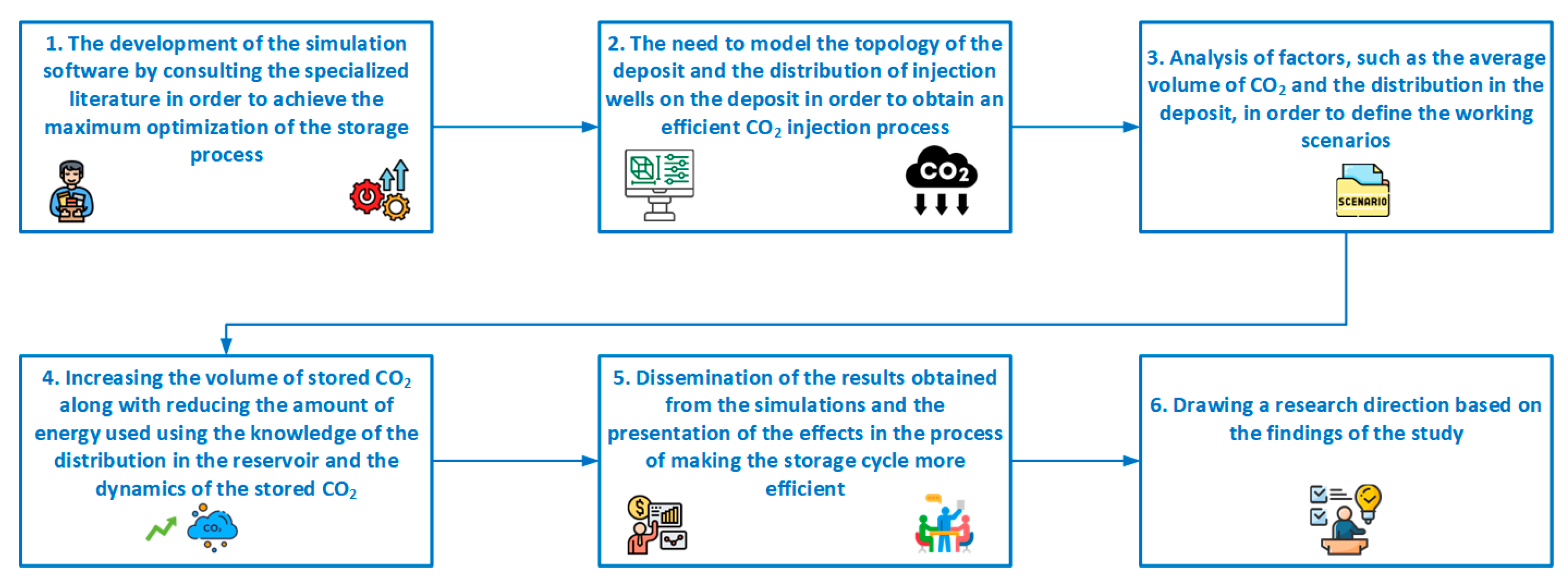
2. Methodology
- The development of the simulation software by consulting the specialized literature in order to achieve the maximum optimization of the storage process;
- The need to model the topology of the deposit and the distribution of injection wells on the deposit in order to obtain an efficient CO2 injection process;
- An analysis of factors, such as the average volume of CO2 and the distribution in the deposit, in order to define the working scenarios;
- Increasing the volume of stored CO2 along with reducing the amount of energy used using the knowledge of the distribution in the reservoir and the dynamics of the stored CO2;
- Dissemination of the results obtained from the simulations and the presentation of the effects in the process of making the storage cycle more efficient;
- Drawing a research direction based on the findings of the study.
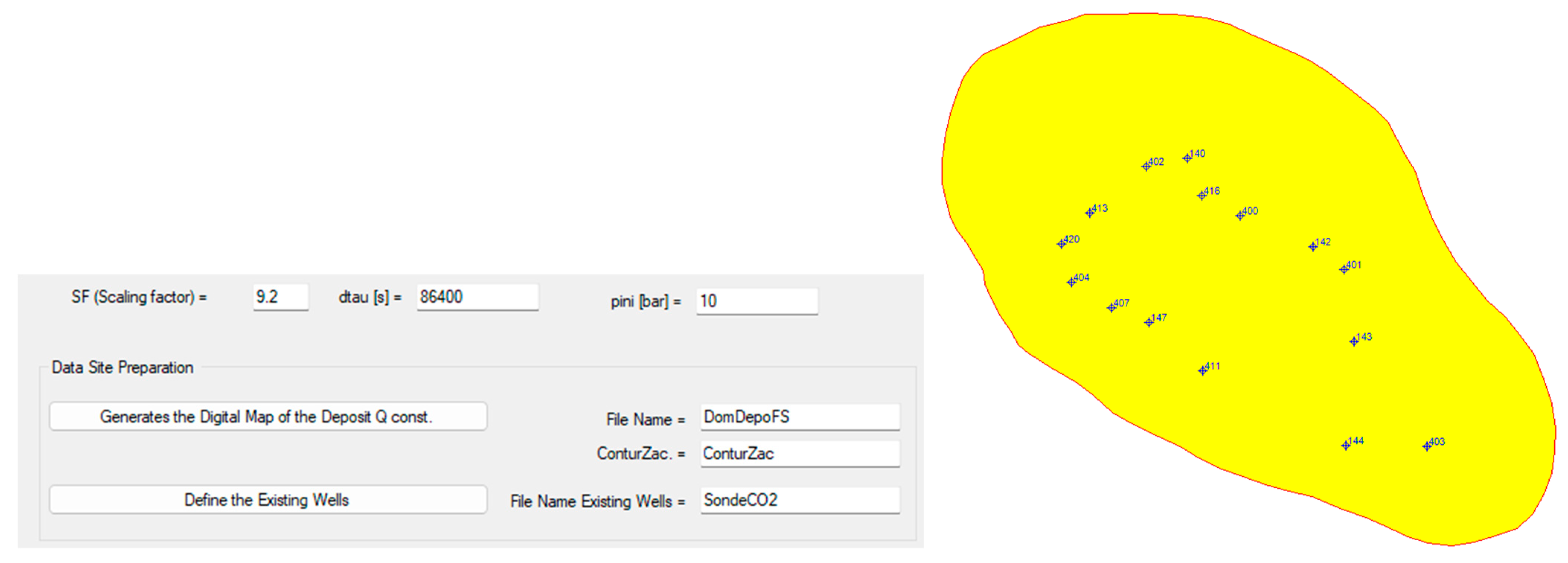
3. Software Description
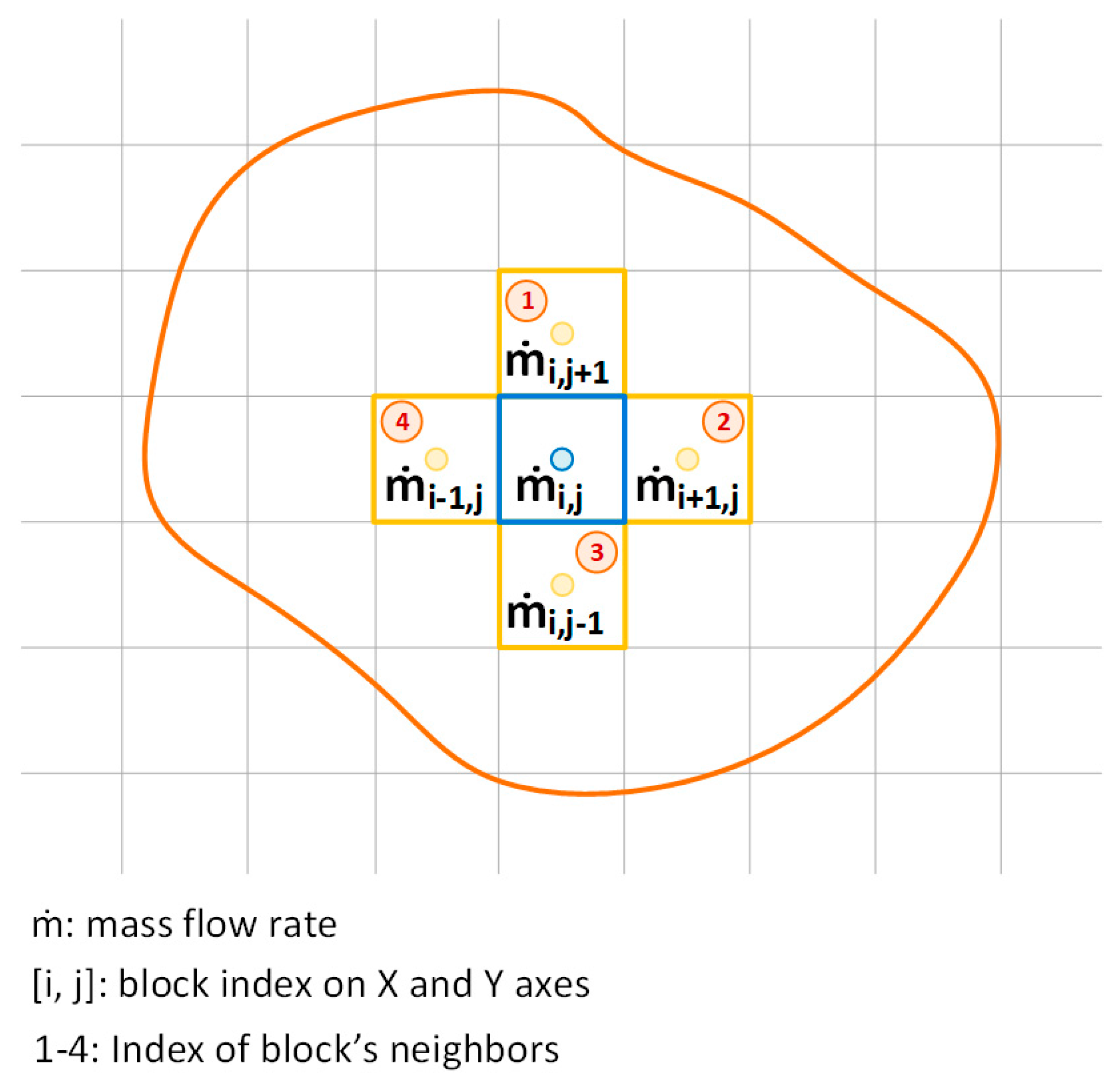
3.1. Short Description of the Model behind the Simulator
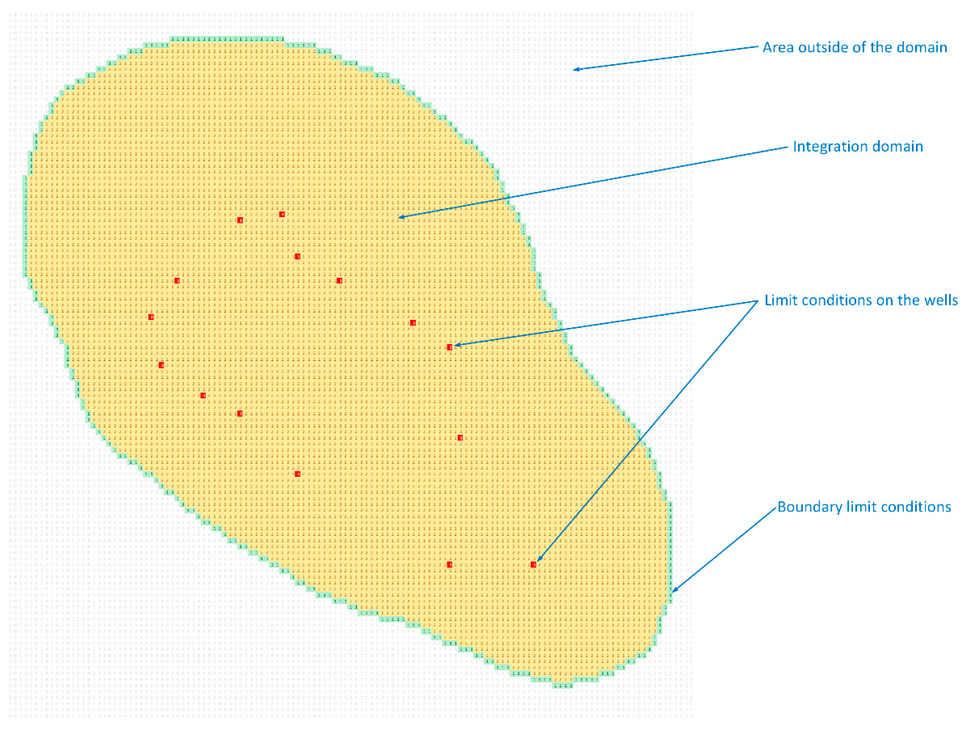
- Imposition of initial conditions on the entire deposit;
- Imposition of boundary conditions in wells and on the boundary;
- Generation of the system of equations related to the geometry of the deposit;
- Solving the system of equations;
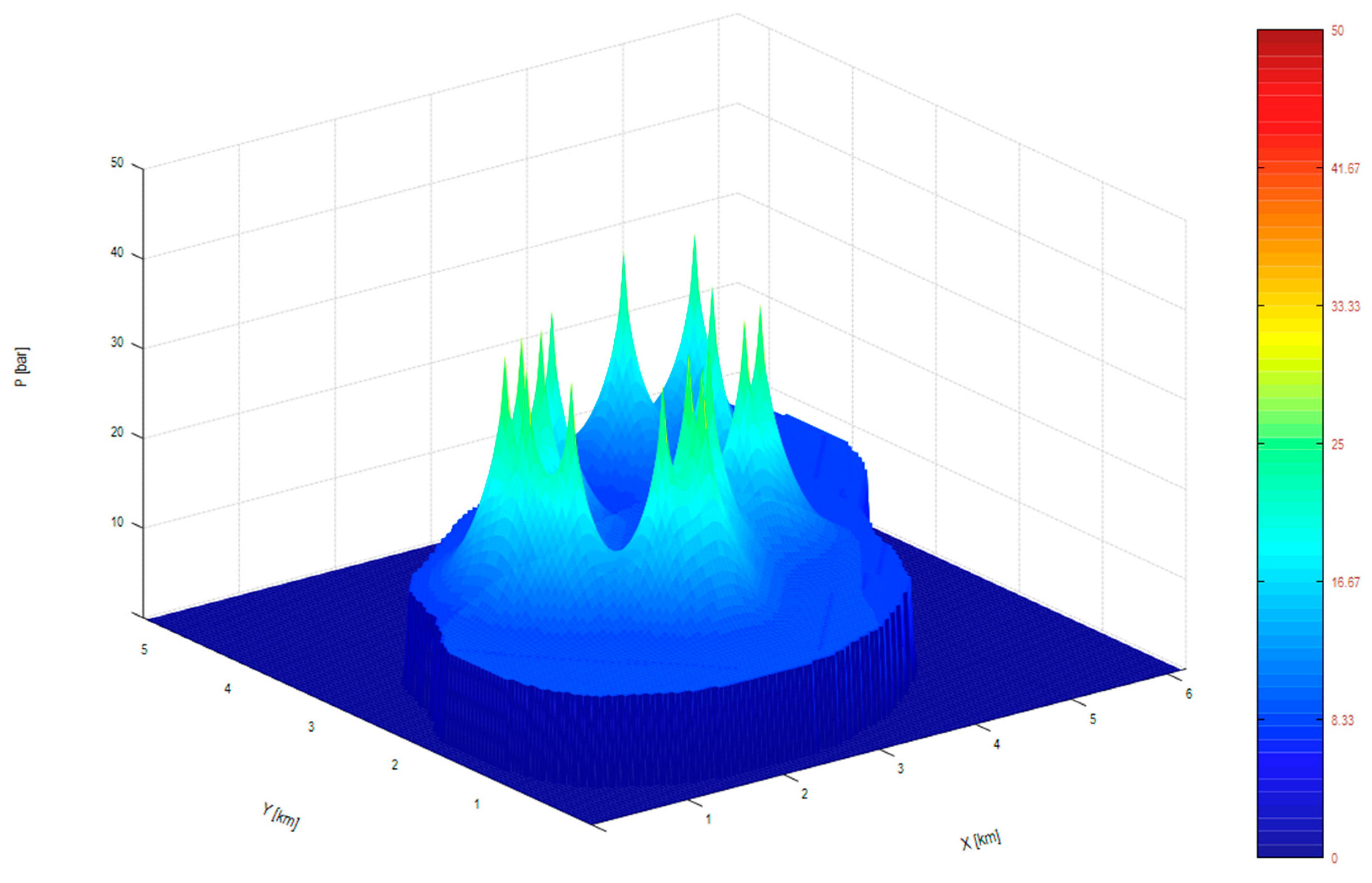
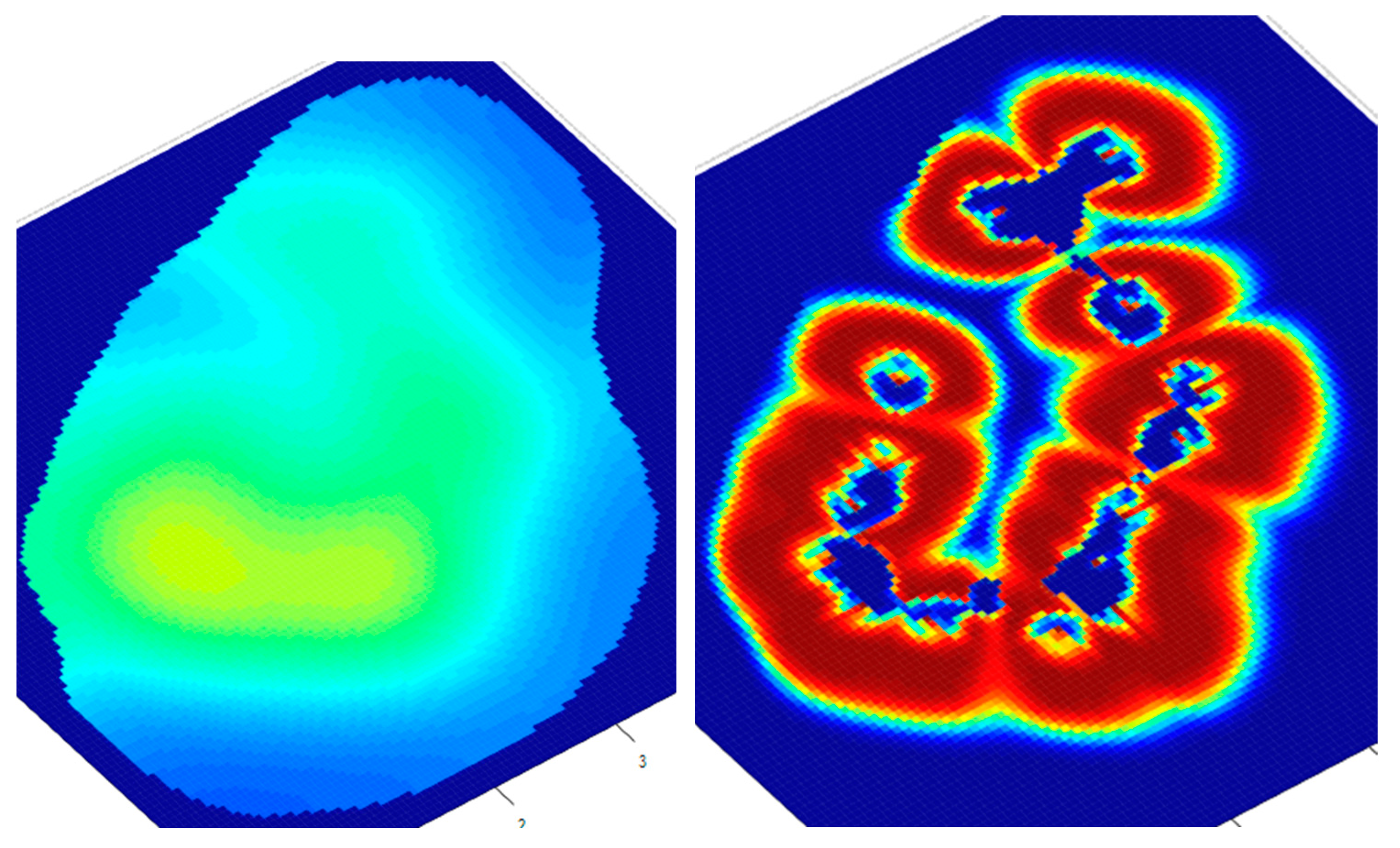
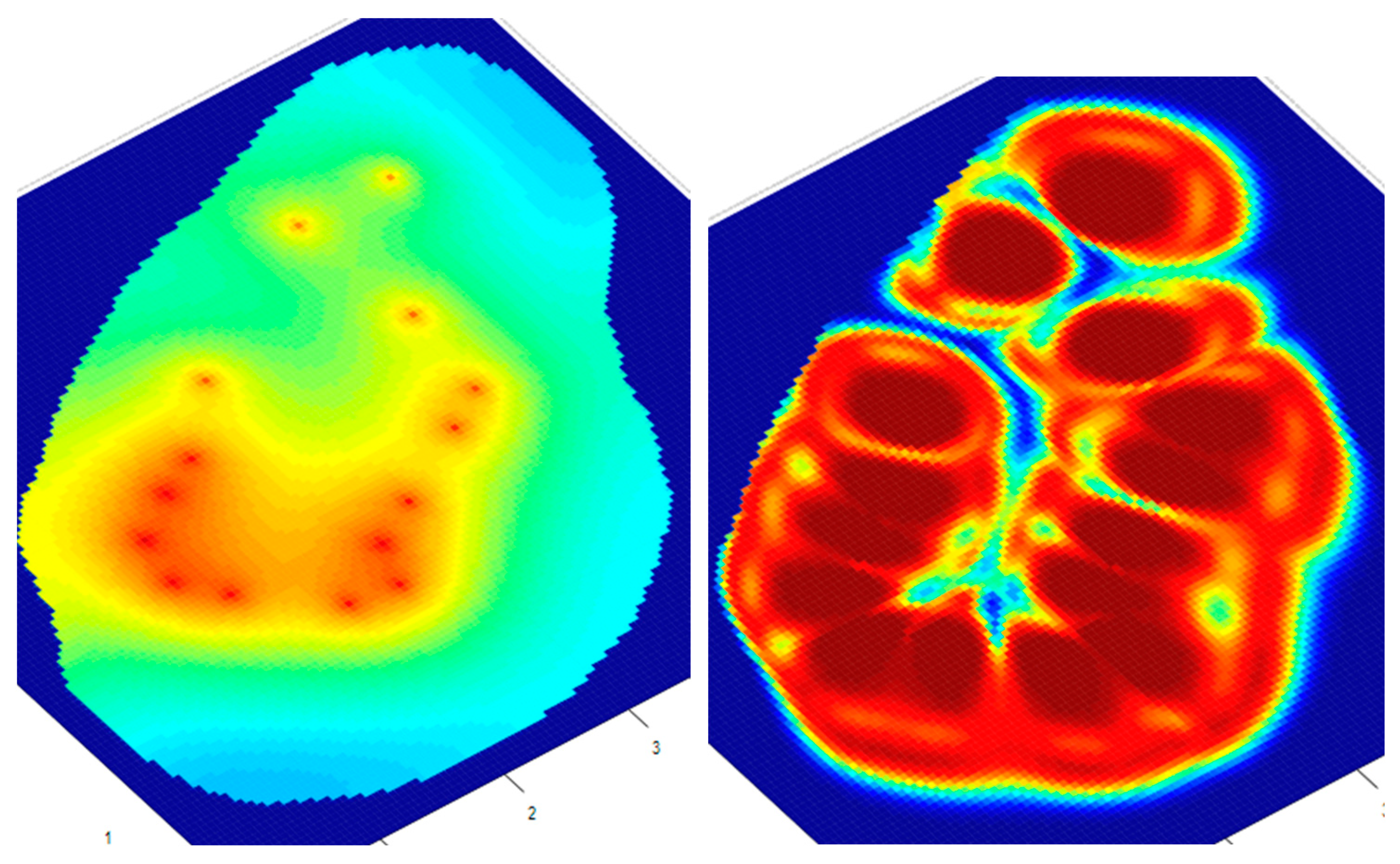
- Generation of the pressure field from the deposit;
- Completion of the next time step and repeat of steps 2–5.
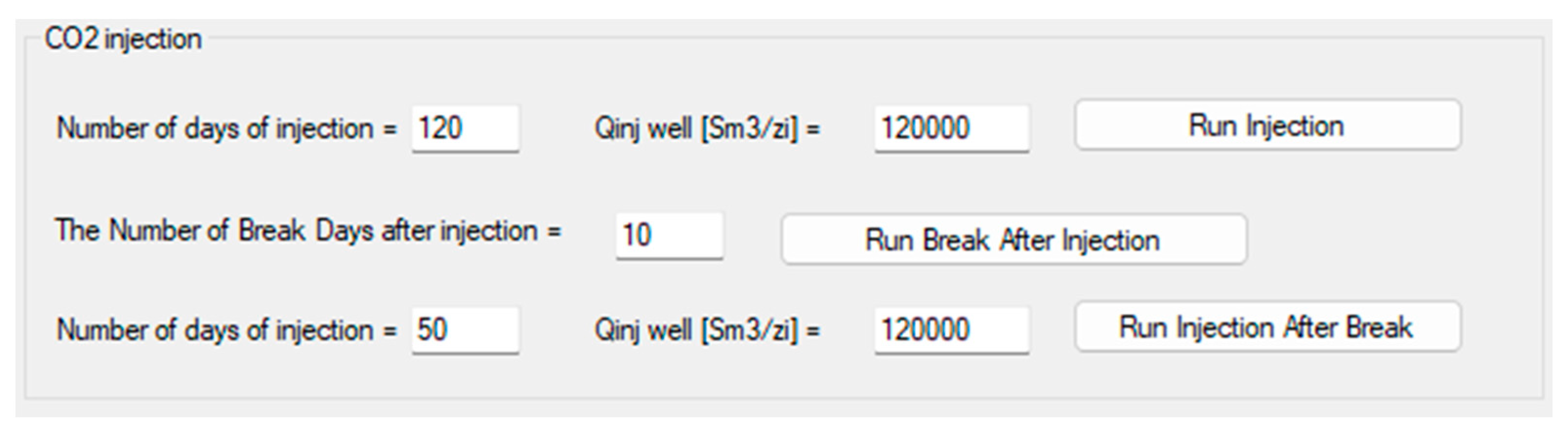
3.2. CO2sim v1 Software Capabilities
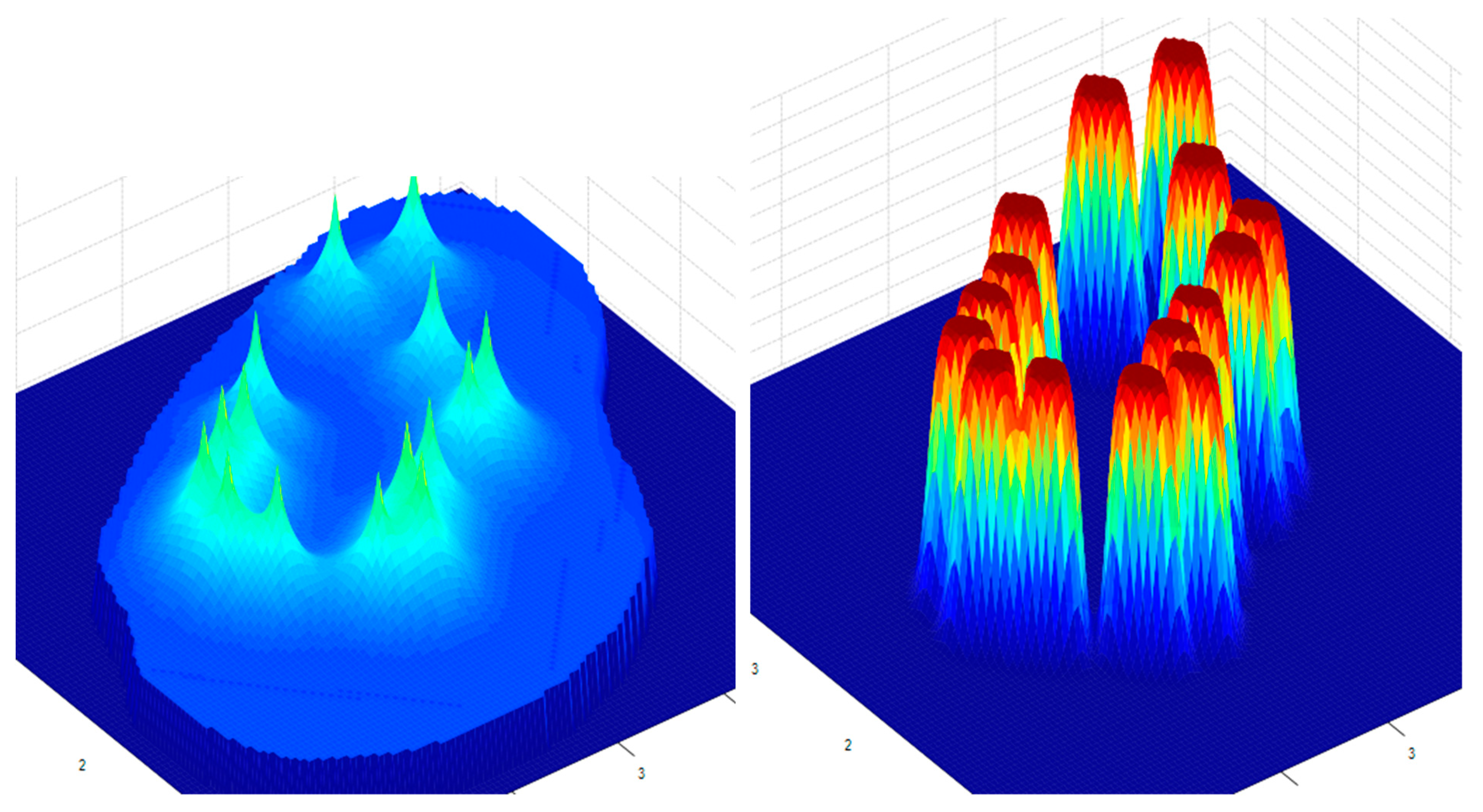
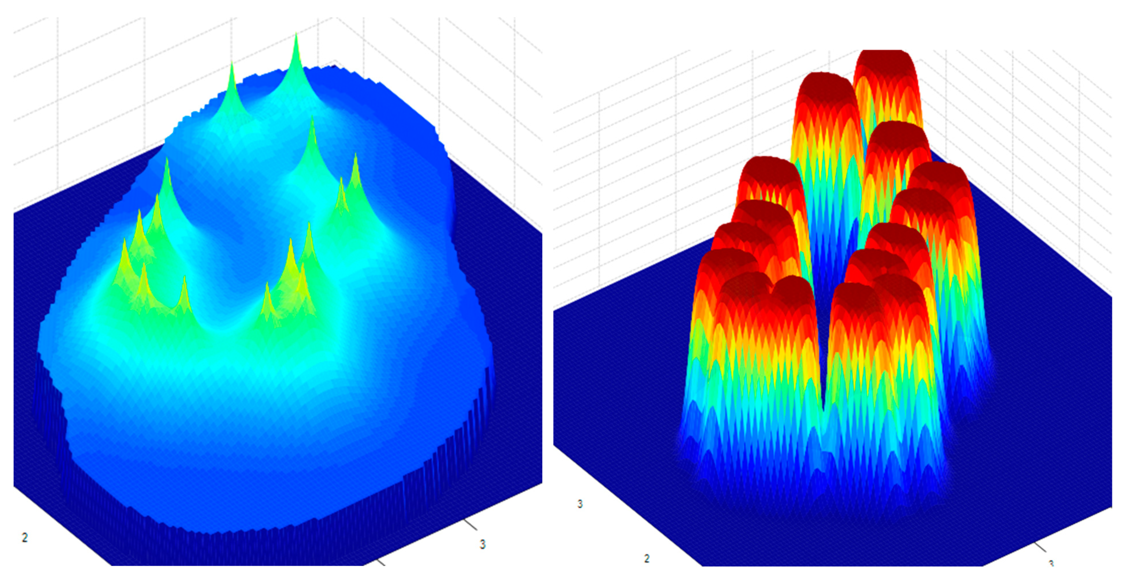
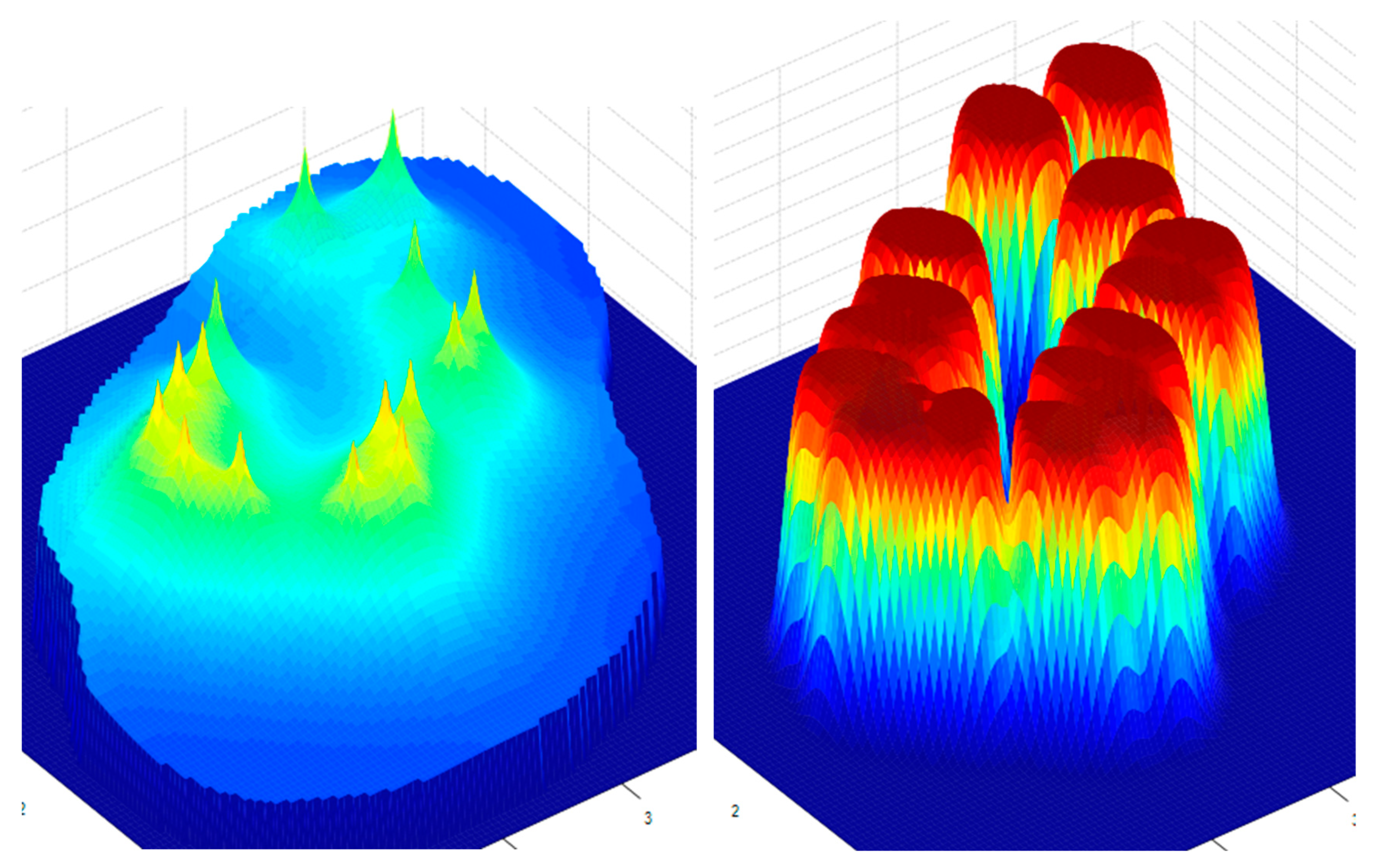
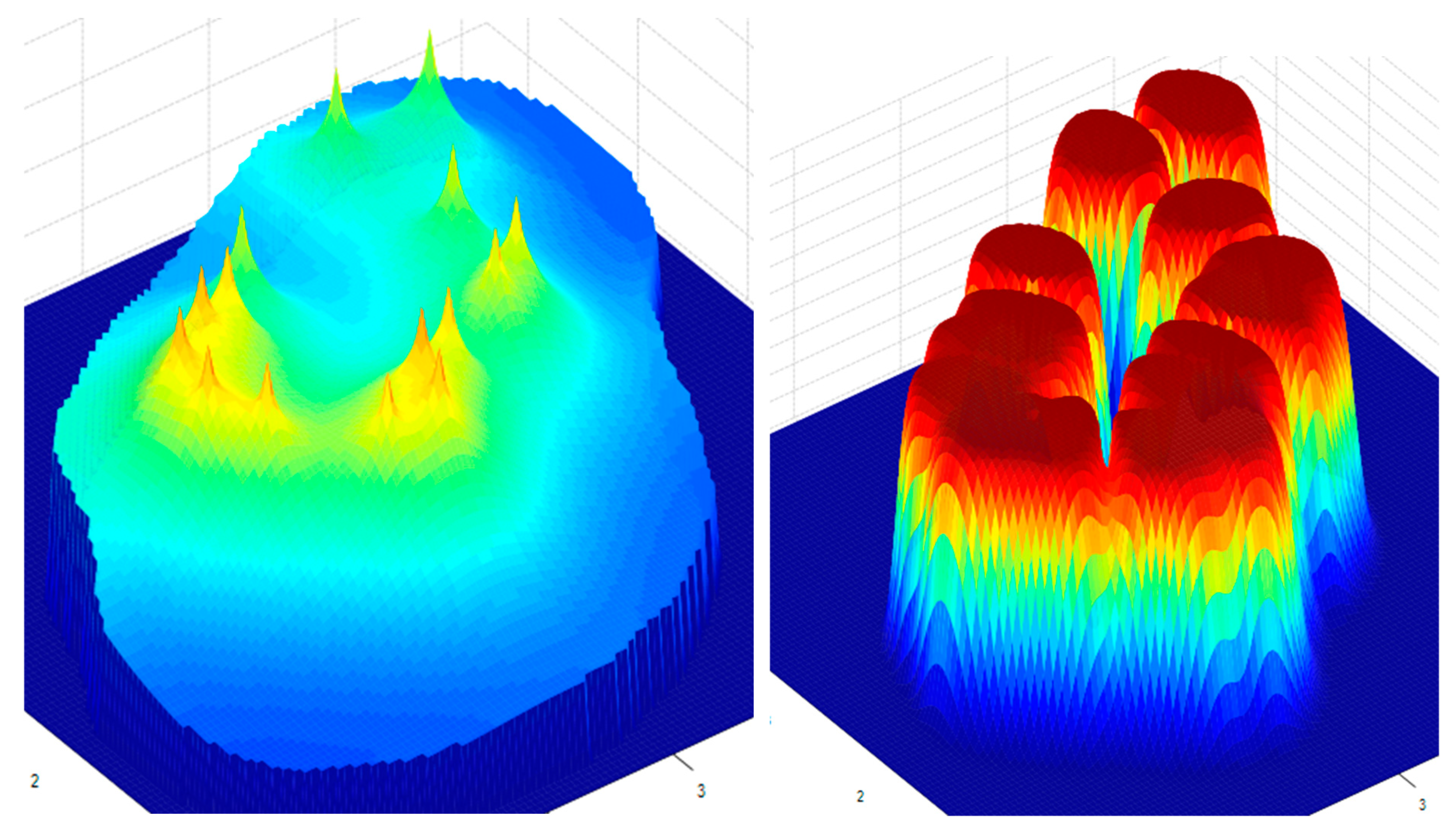
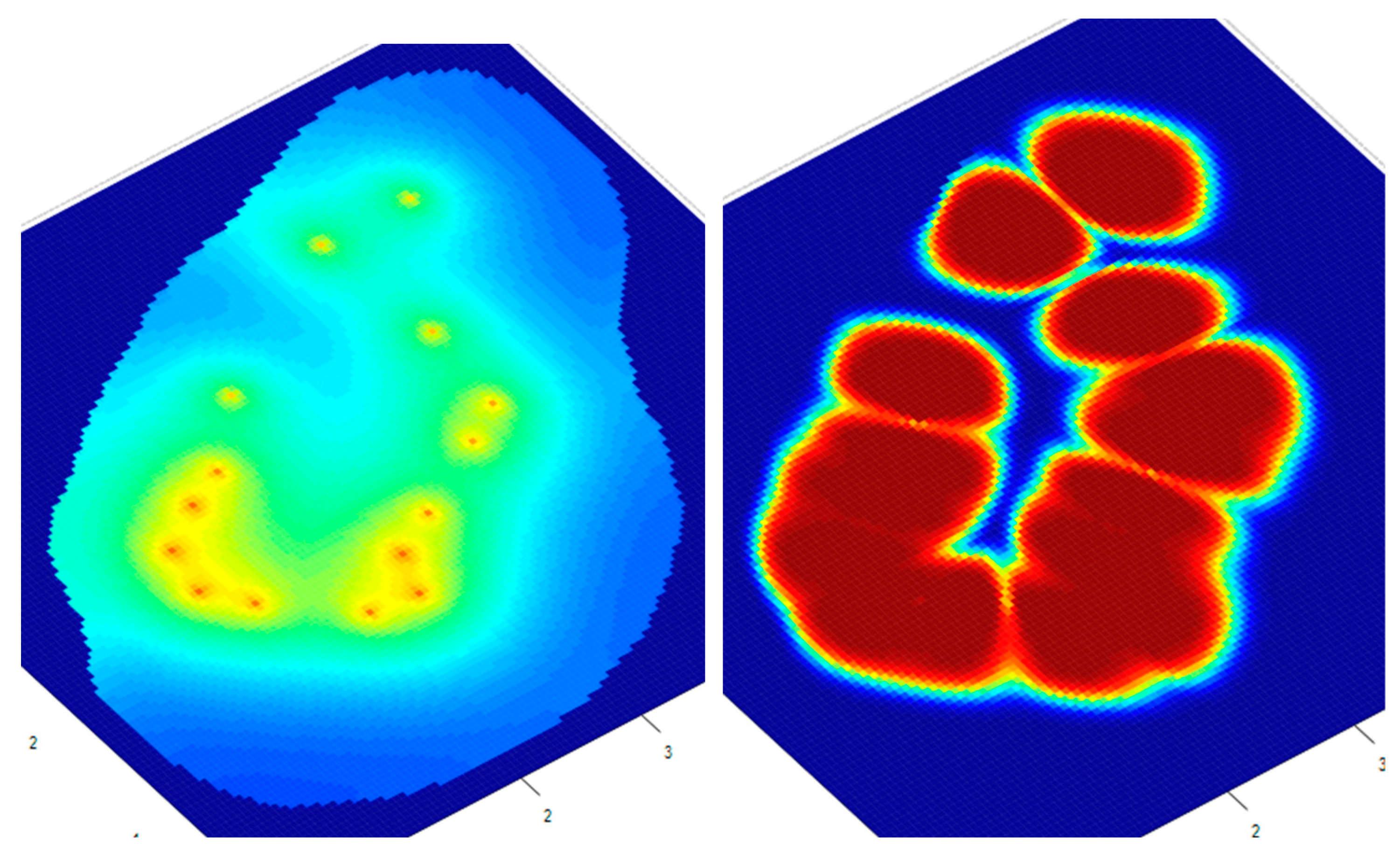
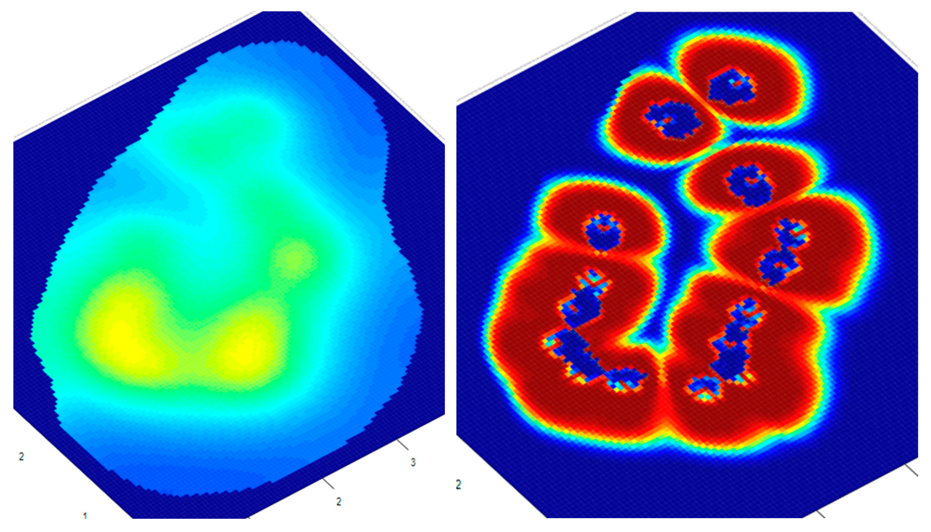
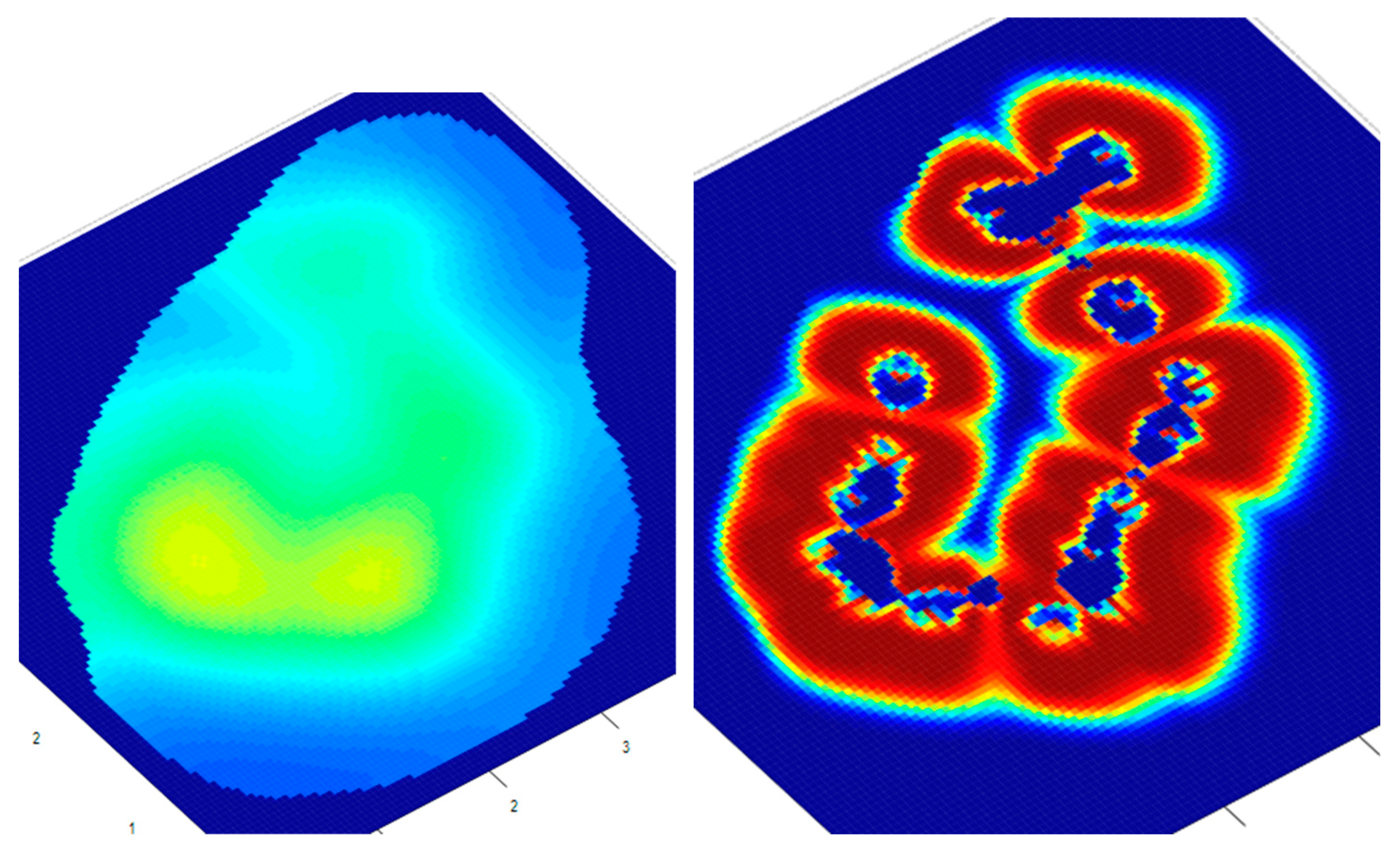
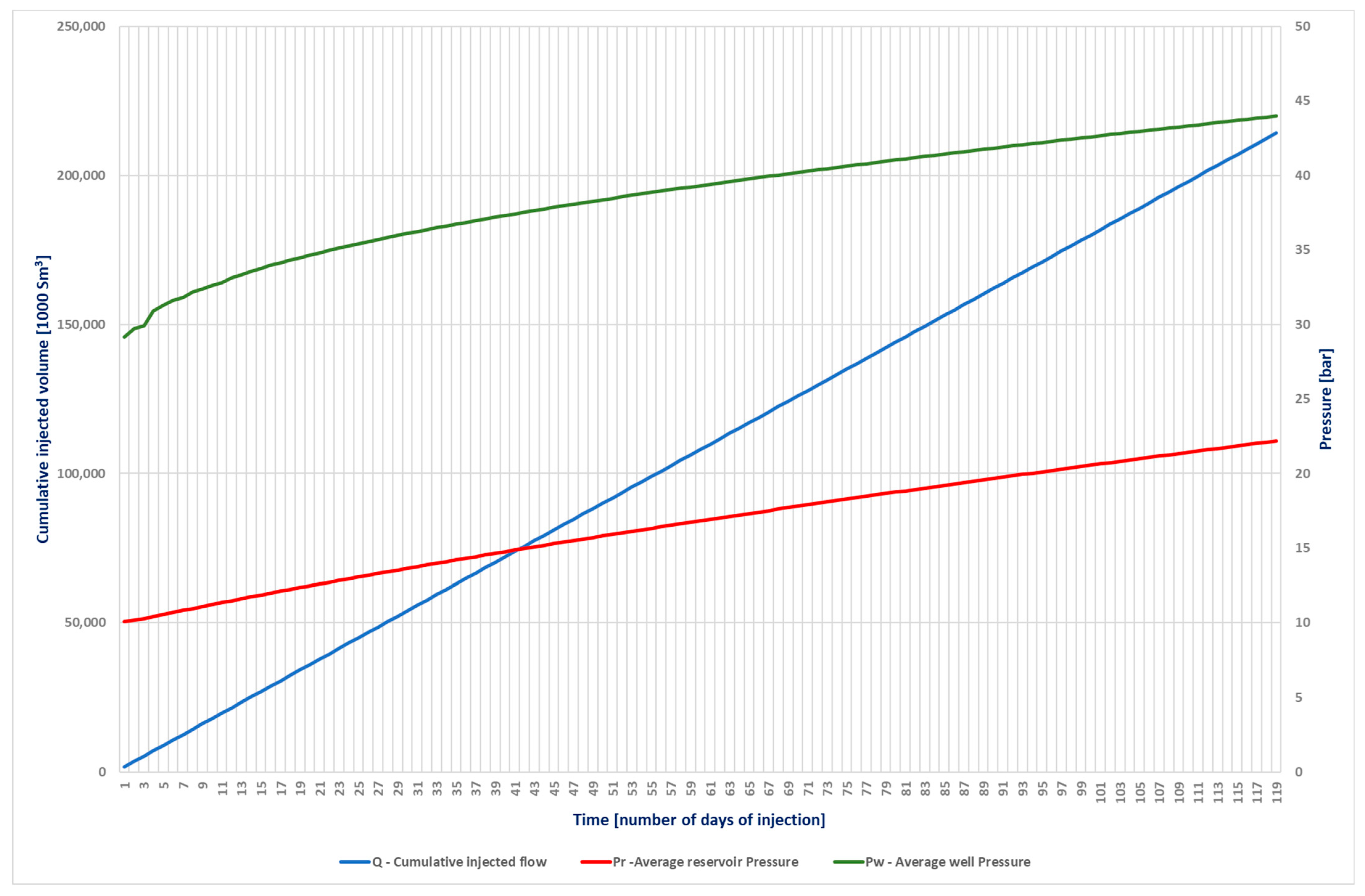
3.3. Outcomes of the Simulation
4. Discussion
5. Conclusions
Author Contributions
Funding
Data Availability Statement
Conflicts of Interest
References
- Rahman, F.A.; Aziz, M.M.A.; Saidur, R.; Bakar, W.A.W.A.; Hainin, M.R.; Putrajaya, R.; Hassan, N.A. Pollution to solution: Capture and sequestration of carbon dioxide (CO2) and its utilization as a renewable energy source for a sustainable future. Renew. Sustain. Energy Rev. 2017, 71, 112–126. [Google Scholar] [CrossRef]
- International Energy Agency. CO2 Emissions in 2023; International Energy Agency: Paris, France, 2024. [Google Scholar]
- Vallero, D.A. (Ed.) Chapter 8—Air pollution biogeochemistry. In Air Pollution Calculations; Elsevier: Amsterdam, The Netherlands, 2019; pp. 175–206. [Google Scholar]
- Ajayi, T.; Gomes, J.S.; Bera, A. A review of CO2 storage in geological formations emphasizing modeling, monitoring and capacity estimation approaches. Pet. Sci. 2019, 16, 1028–1063. [Google Scholar] [CrossRef]
- Intergovernmental Panel on Climate Change. Climate Change 2021—The Physical Science Basis; Intergovernmental Panel on Climate Change: Geneva, Switzerland, 2023. [Google Scholar]
- UNFCCC. Paris Agreement to the United Nations Framework Convention on Climate Change; Phoenix Design Aid: Randers, Denmark, 2015. [Google Scholar]
- IPCC. Global Warming of 1.5 °C IPCC Special Report on Impacts of Global Warming of 1.5 °C above Pre-Industrial Levels in Context of Strengthening Response to Climate Change, Sustainable Development, and Efforts to Eradicate Poverty; Cambridge University Press: Cambridge, UK, 2022. [Google Scholar]
- Martin-Roberts, E.; Scott, V.; Flude, S.; Johnson, G.; Haszeldine, R.S.; Gilfillan, S. Carbon capture and storage at the end of a lost decade. One Earth 2021, 4, 1569–1584. [Google Scholar] [CrossRef]
- Ali, M.; Jha, N.K.; Pal, N.; Keshavarz, A.; Hoteit, H.; Sarmadivaleh, M. Recent advances in carbon dioxide geological storage, experimental procedures, influencing parameters, and future outlook. Earth-Sci. Rev. 2022, 225, 103895. [Google Scholar] [CrossRef]
- Massarweh, O.; Abushaikha, A.S. CO2 sequestration in subsurface geological formations: A review of trapping mechanisms and monitoring techniques. Earth-Sci. Rev. 2024, 253, 104793. [Google Scholar] [CrossRef]
- Bashir, A.; Ali, M.; Patil, S.; Aljawad, M.S.; Mahmoud, M.; Al-Shehri, D.; Hoteit, H.; Kamal, M.S. Comprehensive review of CO2 geological storage: Exploring principles, mechanisms, and prospects. Earth-Sci. Rev. 2024, 249, 104672. [Google Scholar] [CrossRef]
- He, Y.; Liu, M.; Tang, Y.; Jia, C.; Wang, Y.; Rui, Z. CO2 storage capacity estimation by considering CO2 Dissolution: A case study in a depleted gas Reservoir, China. J. Hydrol. 2024, 630, 130715. [Google Scholar] [CrossRef]
- Jitmahantakul, S.; Chenrai, P.; Chaianansutcharit, T.; Assawincharoenkij, T.; Tang-on, A.; Pornkulprasit, P. Dynamic estimates of pressure and CO2-storage capacity in carbonate reservoirs in a depleted gas field, northeastern Thailand. Case Stud. Chem. Environ. Eng. 2023, 8, 100422. [Google Scholar] [CrossRef]
- Raza, A.; Gholami, R.; Rezaee, R.; Bing, C.H.; Nagarajan, R.; Hamid, M.A. CO2 storage in depleted gas reservoirs: A study on the effect of residual gas saturation. Petroleum 2018, 4, 95–107. [Google Scholar] [CrossRef]
- Oh, H.; Yoon, H.; Park, S.; Kim, Y.; Choi, B.; Sun, W.; Jeong, H. Estimation of CO2 storage capacities in saline aquifers using material balance. Fuel 2024, 374, 132411. [Google Scholar] [CrossRef]
- Mortensen, G.M.; Bergmo, P.E.S.; Emmel, B.U. Characterization and Estimation of CO2 Storage Capacity for the Most Prospective Aquifers in Sweden. Energy Procedia 2016, 86, 352–360. [Google Scholar] [CrossRef]
- Li, Q.; Cheng, Y.; Li, Q.; Zhang, C.; Ansari, U.; Song, B. Establishment and evaluation of strength criterion for clayey silt hydrate-bearing sediments. Energy Sources Part A Recovery Util. Environ. Eff. 2018, 40, 742–750. [Google Scholar] [CrossRef]
- Li, Q.; Wang, Y.; Wang, F.; Wu, J.; Usman Tahir, M.; Li, Q.; Yuan, L.; Liu, Z. Effect of thickener and reservoir parameters on the filtration property of CO2 fracturing fluid. Energy Sources Part A Recovery Util. Environ. Eff. 2019, 42, 1705–1715. [Google Scholar] [CrossRef]
- Dumitrache, L.N.; Suditu, S.; Ghețiu, I.; Pană, I.; Brănoiu, G.; Eparu, C. Using Numerical Reservoir Simulation to Assess CO2 Capture and Underground Storage, Case Study on a Romanian Power Plant and Its Surrounding Hydrocarbon Reservoirs. Processes 2023, 11, 805. [Google Scholar] [CrossRef]
- Afolayan, B.; Mackay, E.; Opuwari, M. Dynamic modeling of geological carbon storage in an oil reservoir, Bredasdorp Basin, South Africa. Sci. Rep. 2023, 13, 16573. [Google Scholar] [CrossRef] [PubMed]


| Component | Mmol [kg/m3] | Tk [K] | Pk [bar] | Acc | % vol | % mol | % mas. | % g/Nm3 |
|---|---|---|---|---|---|---|---|---|
| methane | 16.043 | 190.4 | 46 | 0.008 | 98.2608 | 98.2446 | 96.2053 | 704.9346 |
| ethane | 30.07 | 305.3 | 48.84 | 0.098 | 0.7041 | 0.7094 | 1.302 | 9.5405 |
| propane | 44.097 | 369.7 | 42.46 | 0.152 | 0.1954 | 0.1991 | 0.5359 | 3.9268 |
| iso-butane | 58.124 | 408 | 36.48 | 0.176 | 0.0388 | 0.0404 | 0.1433 | 1.0502 |
| n-butane | 58.124 | 425.1 | 38 | 0.193 | 0.0403 | 0.042 | 0.149 | 1.0917 |
| neo-pentane | 72.151 | 469.5 | 33.74 | 0.251 | 0 | 0 | 0 | 0 |
| iso-pentane | 72.151 | 469.5 | 33.74 | 0.251 | 0.0118 | 0.0126 | 0.0553 | 0.4053 |
| n-pentane | 72.151 | 469.5 | 33.74 | 0.251 | 0.0079 | 0.0086 | 0.0378 | 0.277 |
| 2,2-dimethyl-butane | 86.178 | 507.3 | 29.69 | 0.296 | 0 | 0 | 0 | 0 |
| 2,3-dimethyl-butane | 86.178 | 507.3 | 29.69 | 0.296 | 0 | 0 | 0 | 0 |
| 3,3-dimethylbutane | 86.178 | 507.3 | 29.69 | 0.296 | 0 | 0 | 0 | 0 |
| 3-methyl-pentane | 86.178 | 507.3 | 29.69 | 0.296 | 0 | 0 | 0 | 0 |
| 2-methyl-pentane | 86.178 | 507.3 | 29.69 | 0.296 | 0 | 0 | 0 | 0 |
| hexane | 86.178 | 507.3 | 29.69 | 0.296 | 0.0218 | 0.0244 | 0.1282 | 0.9396 |
| 2,4-dimethyl-pentane | 100.205 | 528.6 | 34.98 | 0.453 | 0 | 0 | 0 | 0 |
| 2,2,3-trimethyl-butane | 100.205 | 528.6 | 34.98 | 0.453 | 0 | 0 | 0 | 0 |
| 2-methylhexane | 100.205 | 528.6 | 34.98 | 0.453 | 0 | 0 | 0 | 0 |
| 3-methylhexane | 100.205 | 528.6 | 34.98 | 0.453 | 0 | 0 | 0 | 0 |
| 3-ethyl-pentan | 100.205 | 528.6 | 34.98 | 0.453 | 0 | 0 | 0 | 0 |
| heptane+ | 100.205 | 528.6 | 34.98 | 0.453 | 0 | 0 | 0 | 0 |
| 2,2,4-trimethyl-pentan | 114.232 | 552.3 | 31.23 | 0.491 | 0 | 0 | 0 | 0 |
| n-octane | 114.232 | 552.3 | 31.23 | 0.491 | 0 | 0 | 0 | 0 |
| methyl-cyclohexane | 98.189 | 552.3 | 31.23 | 0.491 | 0 | 0 | 0 | 0 |
| cyclohexane | 82.146 | 528.6 | 34.98 | 0.453 | 0 | 0 | 0 | 0 |
| benzene | 78.114 | 528.6 | 34.98 | 0.453 | 0 | 0 | 0 | 0 |
| toluene | 92.141 | 552.3 | 31.23 | 0.491 | 0 | 0 | 0 | 0 |
| hydrogen | 2 | 33 | 13 | 0 | 0 | 0 | 0 | 0 |
| carbon monoxide | 28.01 | 132.9 | 35 | 0.066 | 0 | 0 | 0 | 0 |
| hydrogen sulfide | 34 | 373.6 | 88.9 | 0 | 0 | 0 | 0 | 0 |
| helium | 4 | 5.2 | 2.26 | 0 | 0 | 0 | 0 | 0 |
| argon | 39.848 | 150.7 | 48.98 | 0 | 0 | 0 | 0 | 0 |
| nitrogen | 28.013 | 126 | 33.94 | 0.04 | 0.4858 | 0.4848 | 0.829 | 6.0741 |
| oxygen | 31.99 | 154.6 | 50.4 | 0.025 | 0.0203 | 0.0203 | 0.0396 | 0.2901 |
| carbon dioxide | 44.01 | 304.1 | 73.76 | 0.225 | 0.213 | 0.2139 | 0.5746 | 4.2101 |
| TOTAL | 100.00 | 100.00 | 100.00 | 732.74 |
Disclaimer/Publisher’s Note: The statements, opinions and data contained in all publications are solely those of the individual author(s) and contributor(s) and not of MDPI and/or the editor(s). MDPI and/or the editor(s) disclaim responsibility for any injury to people or property resulting from any ideas, methods, instructions or products referred to in the content. |
© 2024 by the authors. Licensee MDPI, Basel, Switzerland. This article is an open access article distributed under the terms and conditions of the Creative Commons Attribution (CC BY) license (https://creativecommons.org/licenses/by/4.0/).
Share and Cite
Eparu, C.N.; Suditu, S.; Doukeh, R.; Stoica, D.B.; Ghețiu, I.V.; Prundurel, A.; Stan, I.G.; Dumitrache, L. Software for CO2 Storage in Natural Gas Reservoirs. Energies 2024, 17, 4984. https://doi.org/10.3390/en17194984
Eparu CN, Suditu S, Doukeh R, Stoica DB, Ghețiu IV, Prundurel A, Stan IG, Dumitrache L. Software for CO2 Storage in Natural Gas Reservoirs. Energies. 2024; 17(19):4984. https://doi.org/10.3390/en17194984
Chicago/Turabian StyleEparu, Cristian Nicolae, Silvian Suditu, Rami Doukeh, Doru Bogdan Stoica, Iuliana Veronica Ghețiu, Alina Prundurel, Ioana Gabriela Stan, and Liviu Dumitrache. 2024. "Software for CO2 Storage in Natural Gas Reservoirs" Energies 17, no. 19: 4984. https://doi.org/10.3390/en17194984