Article

Ultra-Short-Term Wind Power Forecasting in Complex Terrain: A Physics-Based Approach

by
Dimitrios Michos
1,*,
Francky Catthoor
2,3,
Dimitris Foussekis
4 and
Andreas Kazantzidis
1
1
Laboratory of Atmospheric Physics, University of Patras, 26500 Patras, Greece
2
Interuniversity Microelectronics Centre (IMEC) vzw, Kapeldreef 75, 3001 Leuven, Belgium
3
ESAT-EE, Katholieke Universiteit (K.U.), 3000 Leuven, Belgium
4
CRES Wind Farm, 19009 Lavrio, Greece
*
Author to whom correspondence should be addressed.
Energies 2024, 17(21), 5493; https://doi.org/10.3390/en17215493
Submission received: 8 October 2024 / Revised: 24 October 2024 / Accepted: 28 October 2024 / Published: 2 November 2024
(This article belongs to the Topic Solar and Wind Power and Energy Forecasting)

Abstract

:
This paper proposes a method based on Computational Fluid Dynamics (CFD) and the detection of Wind Energy Extraction Latency for a given wind turbine (WT) designed for ultra-short-term (UST) wind energy forecasting over complex terrain. The core of the suggested modeling approach is the Wind Spatial Extrapolation model (WiSpEx). Measured vertical wind profile data are used as the inlet for stationary CFD simulations to reconstruct the wind flow over a wind farm (WF). This wind field reconstruction helps operators obtain the wind speed and available wind energy at the hub height of the installed WTs, enabling the estimation of their energy production. WT power output is calculated by accounting for the average time it takes for the turbine to adjust its power output in response to changes in wind speed. The proposed method is evaluated with data from two WTs (E40-500, NM 750/48). The wind speed dataset used for this study contains ramp events and wind speeds that range in magnitude from 3 m/s to 18 m/s. The results show that the proposed method can achieve a Symmetric Mean Absolute Percentage Error (SMAPE) of 8.44% for E40-500 and 9.26% for NM 750/48, even with significant simplifications, while the SMAPE of the persistence model is above 15.03% for E40-500 and 16.12% for NM 750/48. Each forecast requires less than two minutes of computational time on a low-cost commercial platform. This performance is comparable to state-of-the-art methods and significantly faster than time-dependent simulations. Such simulations necessitate excessive computational resources, making them impractical for online forecasting.

1. Introduction

Wind energy is a rapidly growing sector, with the number of operational WTs increasing globally. Accurate and reliable wind energy forecasting is essential for the efficient integration of wind energy into the power grid [1]. This integration facilitates the evolution of energy management techniques, optimizing the usage and storage of diverse energy sources and enabling rapid responses to extreme conditions. Real-time UST wind power forecasting (less than 30 min ahead) is crucial for providing real-time information to human operators for energy management decisions, which optimizes state-of-the-art power grids [2,3,4]. Forecasts with high temporal resolution minimize power losses and grid instabilities while maximizing the positive environmental impact of wind energy. This contributes to reduced volatility in electricity prices and facilitates price reductions through enhanced storage and cost optimization capabilities.
However, forecasting wind movement over complex terrain is particularly challenging because wind speed and direction can change rapidly over short time frames, and the wind field around WTs is complex and three-dimensional. The presence of trees, buildings, and terrain usage in the vicinity of a WT can affect its power production [5]. These environmental factors make accurate forecasting particularly difficult, especially when considering real-time applications.
There are two main types of wind power forecasting models: statistical and physics-based models. Statistical models have the potential for accurate and fast predictions. However, to achieve accuracy, they must be specifically adjusted for different locations and require large training datasets for both indirect power estimation through wind forecasting [6,7] and direct power forecasting [8,9,10,11,12]. This adjustment is not practically realizable for plants with a large number of WTs, where each turbine experiences different terrain and environmental conditions that vary over time. Physics-based models, such as those employing CFD, are predominantly computationally expensive and time-consuming. While they can provide accurate estimations of wind fields at the microscale [13,14,15,16], they are often used offline and are not suitable for real-time UST forecasting. An exception is the work presented in [17], which demonstrates a fast, physics-based UST wind forecasting model for near-coastal (non-complex) flows utilizing multiple Light Detection and Ranging (LIDAR) resolution measurements. CFD models can simulate wind flow around WTs, incorporating necessary structure and terrain information [5,18,19,20]. Additionally, the literature effectively documents the effect of different geometrical structures on wind fields.
To address these challenges, the emergence of hybrid forecasting models [21,22,23,24], which combine statistical and physics-based approaches, offers a promising solution. By leveraging the strengths of both approaches, hybrid models aim to overcome the limitations of each individual type. These models can deliver accurate UST wind energy forecasts while maintaining the computational efficiency required for real-time applications. Hybrid models are essential for tackling the challenges posed by complex terrains, diverse environmental conditions, and the increasing demands for real-time forecasting in modern energy grids.
Numerous data-driven models represent the current state of the art for real-time applications in UST wind energy forecasting (forecasting and monitoring). This research focuses on the physics of wind flow to reduce computational costs and enhance the robustness of the proposed model’s accuracy in response to topographic variations [25,26] as a continuation of the research presented in [5]. This research aims to develop a physics-based model that can readily adapt to terrain changes. The goal is to achieve the accuracy of physics-based models while reducing computational costs to enable fast and reliable forecasts. This approach encourages the scientific community to further explore the potential of CFD [27,28,29,30,31,32,33] for operational wind energy forecasting and accelerates the development and adoption of hybrid forecasting models.
The scope of this work is to incorporate WiSpEx [5] into a framework that can generate UST forecasts of wind power production for a given WT. This modeling approach utilizes wind speed estimations at WT hub height accounting for the wind energy extraction latency of the WT and different turbulence scales through simple and fast averaging techniques. The objective is to achieve a SMAPE of less than 10%. Such a model can operate with limited wind measurements and surface temperature data, simultaneously producing valuable wind data and power forecasts. This approach is applicable to individual turbines in complex environments at a reasonable cost, offering a valuable tool for WF operators seeking to optimize energy production while managing financial considerations.

2. Wind Energy Extraction Latency Model—Theoretical Framework

WTs extract energy based on their design. Due to their momentum, WTs experience a delay in reaching their optimal rotational frequency after a change in wind speed [34,35,36], resulting in a “power lag” or Wind Energy Extraction Latency. This lag, influenced by turbulence and wind gradients, impacts power production. The proposed Wind Energy Extraction Latency model (WEEL) exploits this Wind Energy Extraction Latency to enhance UST power production forecasts by efficiently converting wind speed to power, accounting for wind volatile fluctuations and trend in shorter scales than the predicted power averaging timescale.
Instead of relying on simple averaging of wind speed and power time series, which can lead to a loss of valuable information regarding trends and short-term fluctuations, utilization of specific power curve equations (Section 2.1) combined with high temporal resolution measurements and moving averages (MA) instead of simple averaging is proposed. This approach helps maintain the original sample length while preserving information on key trend characteristics and wind speed volatility.

2.1. Power Curve Equation Modeling

The conversion of wind speed to power is typically accomplished by generating a power curve P f i t from empirical data or using the manufacturer’s specified power curve. The accuracy of the fitted power function and the standard deviation of its error significantly influences the performance of WEEL. To assess WEEL’s performance under realistic conditions, a scenario where the function approximating the power curve captures the primary characteristics of power production but may not fully account for behavior at the extremes of the WT’s operational range is considered. For this purpose, least squares optimization via python is employed to approximate the power curve with a sigmoid function P f i t that was created via mathematical modeling to have the flexibility and interpretability needed for power curve fitting purposes:
P f i t ( x , a , k , b , v , q ) = a + k a 1 + q exp ( b x ) 1 v
where P fit represents power with dimensions [ W ] = [ kg · m 2 · s 3 ] (watts), x is the wind speed with dimensions [ m / s ] (meters per second), a and k are both power terms (lower and upper asymptotes) measured in watts, and b controls the exponential decay rate. Since the argument of an exponential function must be dimensionless, b x is dimensionless. Given that x has dimensions of [ m / s ] , b must have dimensions [ s / m ] , which is the inverse of speed. v and q are dimensionless quantities used for scaling and shaping the curve.
The optimal parameters were determined using a least squares fitting using 10 MA Wind speed data (x) and corresponding 15 ma power output data (y) for curve fitting via curve_fit function in python. Least squares optimization fits a model to data by minimizing the sum of squared differences between observed and predicted values. The objective is to find model parameters that make predictions as close as possible to actual observations. Given observed data points ( x i , y i ) , where x i is the input (e.g., wind speed) and y i is the output (e.g., power), a model function f ( x , θ ) is fitted to these points. Here, θ represents the model’s parameters. The function f ( x , θ ) predicts the output y for a given input x. The fit is evaluated with the usage of Sum of Squared Errors (SSE), defined as follows:
SSE = i = 1 n y i f ( x i , θ ) 2
where n is the number of data points. The SSE quantifies the total squared deviation of the model’s predictions from the observed data. A smaller SSE indicates a better fit.
The optimization process starts with an initial estimate of the parameters θ . The model calculates predicted values f ( x i , θ ) for each data point x i , and the SSE is computed. The parameters θ are iteratively adjusted to minimize the SSE, often using algorithms like gradient descent. This continues until the SSE is minimized or converges. The resulting parameters θ provide the best possible fit of the model to the data [37].
This fitting approach ensures the derived power function accurately reflects the WT’s behavior, making it useful for modeling power output based on wind speed. Understanding the modeled problem is essential for optimizing WT performance and enhancing wind energy production efficiency.

2.2. ShiVa Detection

This model uses n-minute MA or n-MA for the wind speed series and m-minute MA or m-MA for the wind power output, where m , n ϵ N , and m > n , to effectively reveal the power production latency and the averaging effects on WT power and wind speed, assuming a resolution Δ t . The rationale behind the different averaging window sizes lies in the inherent trade-off between volatility and trend robustness.
The first part of the model is the conversion of horizontal velocity magnitude u at hub height of a WT to power with proper selection of power curves ( P ( u ) ). Power curves can be produced by continuous functions approximated to operational data or be obtained by manufacturers. Complex power curve models account atmospheric conditions that affect the power output of a WT, as presented by [38]. In this study, the usage of continuous functions approximated to operational data is examined.
After selecting m , n and the power function P , which is approximated to the measurement data, the identification of the Wind Energy Extraction Latency of a WT is possible. This process is called Wind Optimal Shift-Value(ShiVa) identification. If u t n is the n-MA horizontal wind speed magnitude and P t m is the m-MA power, the estimated power is calculated as follows:
P ¯ t m = P ( u t n )
The wind speed measurements u t n are iteratively shifted forward by Δ t , creating a series of shifted series. For each shift i ϵ N , the power P ¯ t m i is estimated by using the shifted wind speed u t n i . Any metric can be applied to evaluate P ¯ t m i with respect to P t m .
By detecting the i value that optimizes the selected metric, the latency of the WT i Δ t is found. This shift value (ShiVa) is called Optimal ShiVa and is notated by i o p t . Additionally, the maximum ShiVa i m a x is determined, representing the largest shift where the metric’s evaluation is the best approximation for power P ¯ t m 0 = P ¯ t m , estimated by the unshifted series. i m a x represents the maximum shift that can be applied to u t n without raising the error variance more than the initial estimation:
| P ¯ t m 0 P ¯ t m i m a x | | P ¯ t m 0 P ¯ t m i | , i ϵ N
In reality, the actual optimum and maximum ShiVas are not natural numbers most of the time. In numerical solving, where continuous variables are never available, researchers can simply select the best approximation according to the initial resolution of the data. This method enables WEEL to directly produce UST forecasts in extremely short horizons quickly and directly by applying a power curve transformation to WEEL’s maximum ShiVa shifted wind speed series to obtain P ( u t i m a x ) .
WEEL uses the ShiVas to minimize the error variance from power conversion and/or extend the forecasting horizon of a forecasting module, by converting the wind speed forecast to power. It is worth noting that after ShiVa detection is complete, Wind speed series from physics-based and data-driven forecasting models can be shifted by i m a x and used as inputs of the selected power curves to generate the final power forecast output.
Many error metrics are present in the literature. In this study, the most commonly used metrics are minimized: mean absolute error (MAE), mean squared error (MSE), root mean squared error (RMSE), and mean absolute percentage error (MAPE). This metric selection showcases that different metrics evaluating the error behavior (e.g., in terms of measurement units, percentage) are minimized at the same optimal ShiVa:
MAE = 1 N i = 1 N y i y ^ i
MSE = 1 N i = 1 N ( y i y ^ i ) 2
RMSE = 1 N i = 1 N ( y i y ^ i ) 2
MAPE = 1 N i = 1 N y i y ^ i y i 100 %
where y ^ i is the forecasted value and y i is the measured and y i y ^ i is the absolute error. It is worth mentioning that some metrics are expected to obtain a maximum value (like correlation) at the optimal ShiVa.

3. Data and Methodology

3.1. CRES Wind Farm

The presented model’s performance is validated with real data from the Centre for Renewable Energy Sources and Saving (CRES) WF, which is located at Lavrio, Greece (37.76, 24.06). CRES provided a Digital Elevation Model (DEM) file, which contains elevation data for the terrain. The DEM file was used to create the geometrical representation and construct the domain for the CFD simulations. Wind LIDAR measurements at nine different heights (40 m, 54 m, 78 m, 100 m, 120 m, 140 m, 160 m, 180 m, 200 m) and power output data from two WTs shown in Table 1, from a LIDAR campaign that took place between 22 October and 24 October 2010 [39] were used for this study. CRES also provided horizontal wind speed measurements at hub height from both WTs. These measurements were taken during the LIDAR campaign. Wind speed at the WT hub height is measured by anemometers mounted directly on the hub and corrected online by the WT manufacturers.

3.2. WiSpEx

For this study, the results of the Wi.Sp.Ex. model presented in [5] are utilized as input data to forecast the power production of the Enercon and NEG WTs. Wi.Sp.Ex. is a physics-based model that spatially extrapolates wind measurements over complex terrain capable to sufficiently capture the effects of terrain curvature on wind flow. The model extrapolates wind speed based on the hypothesis that stationary solutions of CFD equations can accurately represent wind flow over complex terrain.
In steady-state (or stationary) CFD simulations, the solution aims to reach a stable point where the flow properties (like velocity, pressure, etc.) no longer change with time [18,19]. This means the governing equations, like the Navier–Stokes equations, are solved assuming that time derivatives are zero. Since the solution is not evolving in time, once convergence is achieved, it reflects a single, stable flow field. As a result, steady-state simulations are less sensitive to mesh changes because the solution is not influenced by time-stepping errors or transient effects. The primary concern is resolving spatial gradients, so mesh refinement directly addresses spatial accuracy. In contrast, time-dependent simulations must accurately capture both spatial and temporal variations, leading to greater sensitivity to mesh quality and the need for temporal resolution. Figure 1c shows the meshing of the simulation domain, while Figure 1d illustrates the ability of Wi.Sp.Ex. to capture the effect of terrain curvature on the wind flow. The location of the LIDAR, the WTs, and the terrain characteristics are shown in Figure 1a,b.

3.3. WEEL

The proposed method is designed for UST power production forecasts, specifically within the 5 to 30 min range. While direct regression techniques are more suitable for shorter-term predictions, this method effectively addresses the “tens of minutes”-scale forecasting horizon, crucial for online micro-grid energy management and trading strategies. For longer-term forecasting needs, a combination with probabilistic NMP-based methods is recommended. The operational and trading significance of 15 min power production forecasting defines the power series averaging window. 10 min averaging window for wind speed series is employed, matching the WiSpEx results. 10 min MAs are slightly faster and more volatile, which is advantageous during ramp events. 1 min resolution 10-MA wind speed measurements and 15-MA power measurements are used to pinpoint the Optimal ShiVa offset of wind speed series that minimizes the standard deviation with respect to their fitted power curve and the Maximum ShiVa, defining the maximum allowable shift of the 10-MA horizontal wind speed magnitude time-series.
WEEL utilizes WiSpEx as the forecasting module, assuming that there is a phase error due to air travel distance from the inlet of the simulations to the WTs. The actual phase error depends on wind speed and the distance between the measurement location and the WT. WiSpEx’s maximum phase error for the 10 min simulated flow is expected to be below 10 min from the inlet of the simulations presented by [5]. Such a scenario is possible in WFs where measurement instruments are not optimally located for the proposed modeling approach, as is the case with the CRES WF. By assessing the model’s performance in this realistic, non-optimal scenario, This study aims to establish a benchmark for WEEL’s effectiveness in practical applications.
The assessment of WEEL’s performance in this non-optimal scenario, is conducted by estimating 15 min power output after a full 15 min step by averaging WiSpEx’s Max-ShiVa shifted series with the unshifted 10-MA measured wind speed at the hub height of the Enercon and Neg WTs and converting it to power with a power curve equation, accounting for persistence in wind speed. Additionally, 5 min ahead 15 min power is calculated directly with WEEL by Max ShiVa shifting the 10-MA wind measurements. Simple linear interpolation is used to calculate the 10 min ahead 15 min power output. It is important to note that the averaging lengths for WEEL input/output (wind speed and power) are operator-defined and not fixed to this case study. Similarly, WiSpEx can be used for different averaging windows. WEEL’s flow chart is shown in Figure 2.
To validate the performance of power forecasting, metrics like SMAPE are frequently preferred over MAPE to mitigate the influence of extreme errors. Moreover, normalized values such as Normalized Root Mean Square Error (NRMSE) and Normalized Mean Absolute Error (NMAE) are employed to provide a generalized perspective of model behavior across diverse datasets like in [9,10,11,12]. Formally, NRMSE and NMAE can be expressed as:
NMAE = MAE P r a t e d
NRMSE = RMSE P r a t e d
where P r a t e d signifies the rated or maximum power output of a given WT.SMAPE, a widely adopted metric in power forecasting, is defined as:
SMAPE = 1 N i = 1 N y i y ^ i | y i | + | y ^ i | 2 100 %
In this equation, y i represents the forecasted value, while y ^ i denotes the corresponding actual value.

4. Results

In this section the results from WEEL are discussed and compared with state-of-the-art models and persistence. Recent years have witnessed a surge in the development of UST wind power forecasting models, with a majority leaning towards statistical approaches as exemplified by [9,10,11,12].

4.1. Shiva Detection

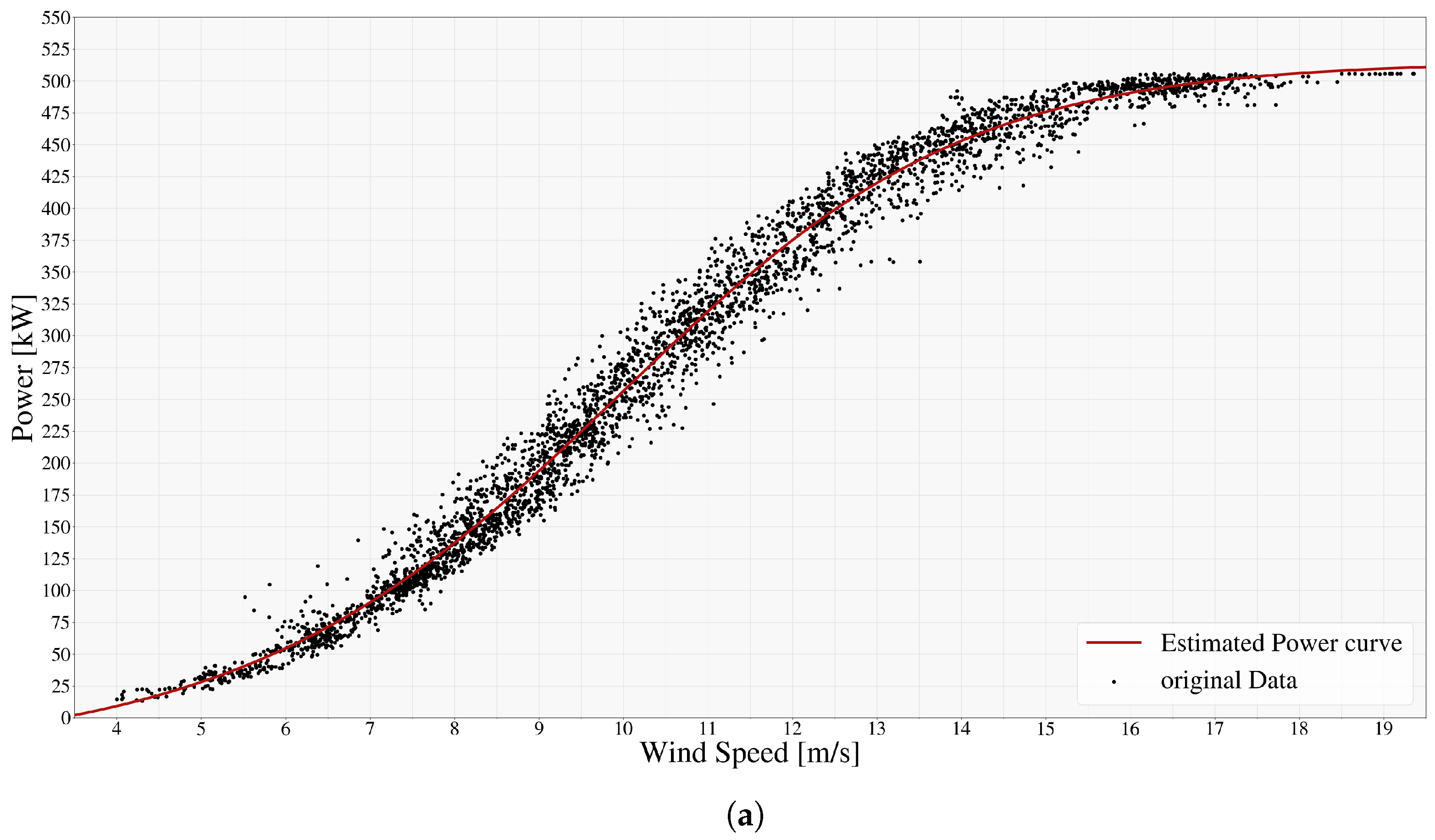
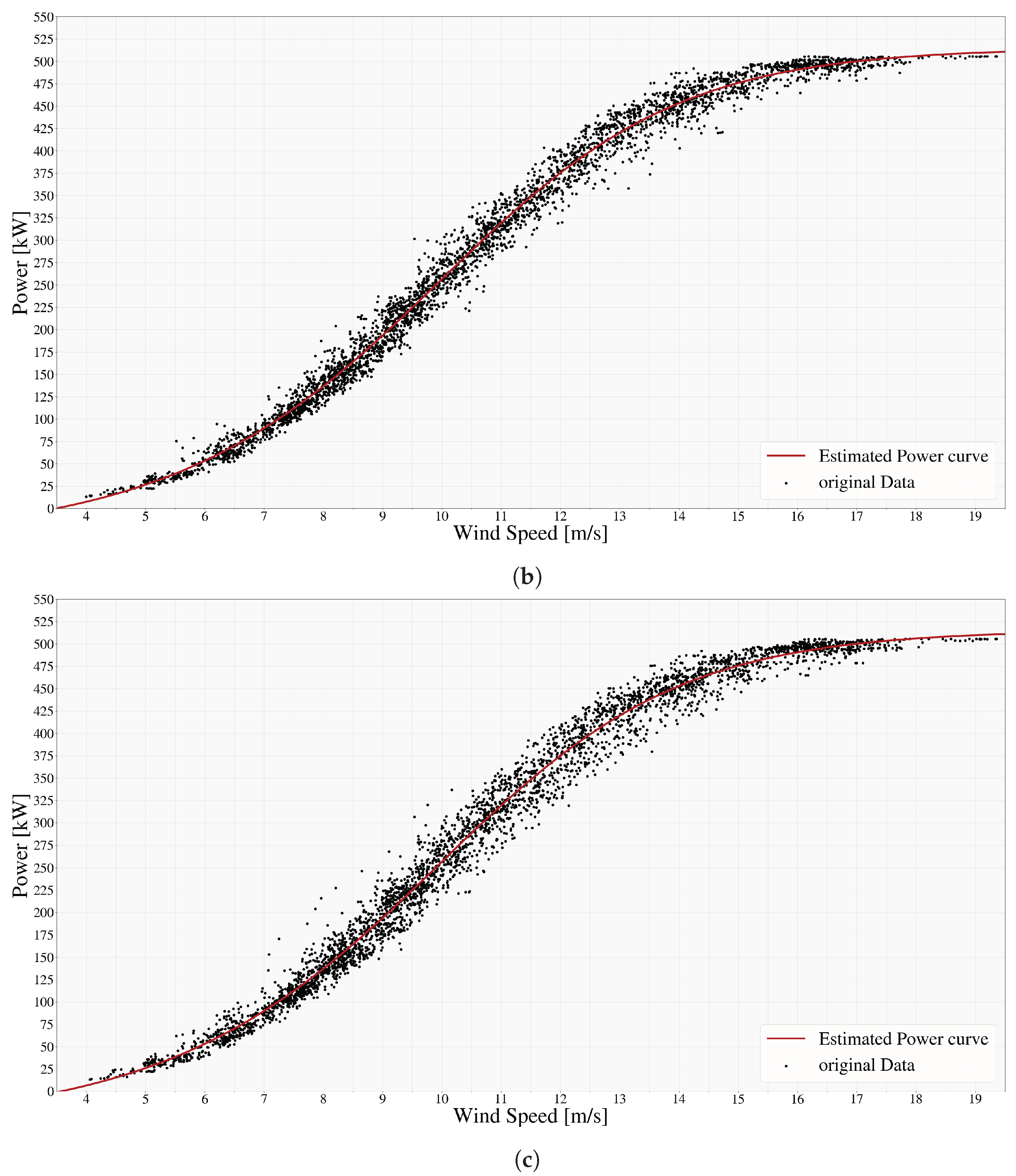
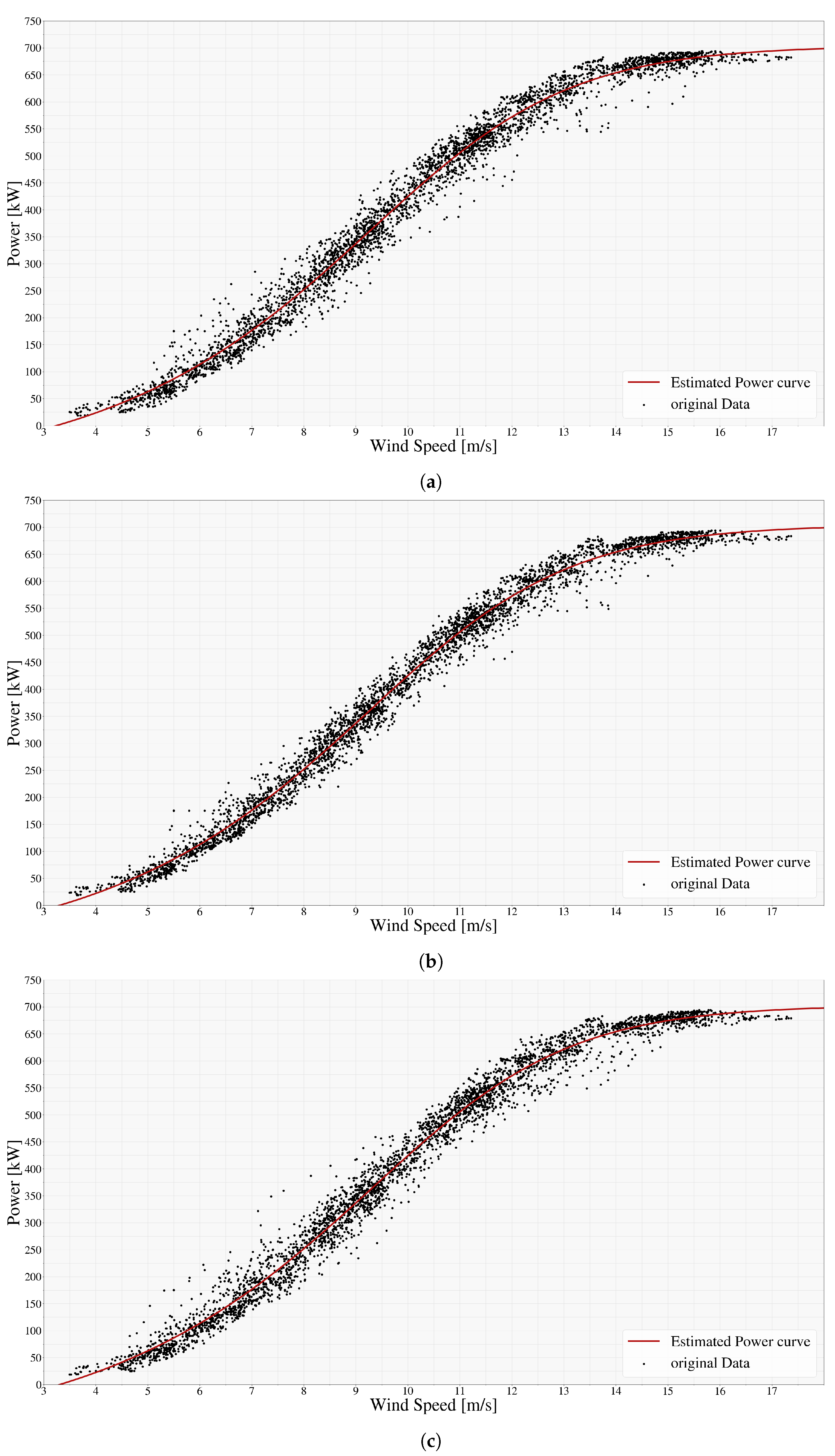
Table 2 and Table 3 provide the metric evaluation for Enercon and NEG WTs. The optimal ShiVa for Enercon WT is +3 min while for NEG WT the Optimal ShiVa is +2 min, demonstrating the lowest MAE, MSE, and RMSE, respectively. Enercon WT exhibits a larger “power lag” compared to the NEG WT, potentially due to differences in size, design, turbulence, or power curve modeling errors. The maximum allowable shift for NEG is +5 min setting the limits for both WTs, suggesting that a 5 min shift does not raise the power conversion errors for both WTs.
A visual scatter plot inspection (Figure 3 and Figure 4) validates the values of error metrics (Table 2 and Table 3). Shiva detection helps mitigating the volatility produced through the power conversion by shifting the wind speed series forward by the determined Optimal ShiVa. Once the optimal ShiVa is established, the estimation of 15 min power production with a max ShiVa-minute lead time is possible, and the final power curve can be selected. This methodology is valuable for capturing power production during rapid changes in wind speed without incurring a significant computational burden.
After ShiVa detection is complete, WEEL uses WiSpEx to extrapolate LIDAR wind speed to the WTs’ hub height, obtaining 10 min averaged wind speed forecasts. The resolution of Maximum ShiVa shifted forecasts is enhanced to 5 min using linear interpolation, while the max ShiVa shifted 10 MA wind speed measurement series are downgraded to 5 min. The WEEL 15 min ahead power forecast is then produced by converting the forecasted wind speed to power production via the power curve for each WT as described in Section 2. This simple yet effective and fast approach (Figure 2), incorporates the WT’s momentum and possible persistence, resulting in WEEL’s forecasted 10 MA averaged wind speed. This wind speed is converted to 15 min power using the fitted power curve, providing the final 15 min ahead power output forecast for the WTs. This version of WEEL can be considered a hybrid CFD–momentum model accounting for wind speed persistence.

4.2. Power Forecasting

4.2.1. Enercon

Table 4 summarizes the performance of WEEL in predicting power output at different time steps. Notably, the SMAPE remains consistently below 10% for all prediction horizons, indicating sufficient accuracy despite the simplification of the study [5]. The choice between MAPE and SMAPE as evaluation metrics is discussed, emphasizing SMAPE’s robustness in handling low- or zero-power output scenarios, which are common in wind power forecasting. WEEL, incorporating persistence effects, coupled with WiSpEx, demonstrates superior performance compared to both persistence forecasting and standalone WiSpEx(+15 min time step). This is evidenced by consistently lower MAPE and SMAPE values, particularly at the critical 15 min-ahead forecast horizon, which is valuable for grid management and energy trading, where WEEL achieves an impressive MAPE of 8.44% in contrast with persistence’s 15.03% MAPE value, showcasing its success in challenging scenarios.
At the 5 min horizon, WEEL directly utilizing a 10 min wind speed MA demonstrates a MAE of 12.23 kW and RMSE of 16.47 kW, showing slightly better performance compared to persistence forecasting (MAE: 15.32 kW, RMSE: 21.21 kW). Extending the prediction to 10 min, WEEL power linearly interpolated by adjacent steps maintains its advantage (MAE: 12.96 kW, RMSE: 17.75 kW) compared to persistence (MAE: 24.85 kW, RMSE: 34.47 kW). Combining WEEL with WiSpEx at the 15 min horizon further improves upon persistence. At this critical forecast step, WEEL coupled with WiSpEx delivers the best performance (MAE: 17.81 kW, RMSE: 23.08 kW), significantly outperforming persistence (MAE: 31.82 kW, RMSE: 44.03 kW) and Direct WiSpEx forecasts (MAE: 31.58 kW, RMSE: 40.54 kW).
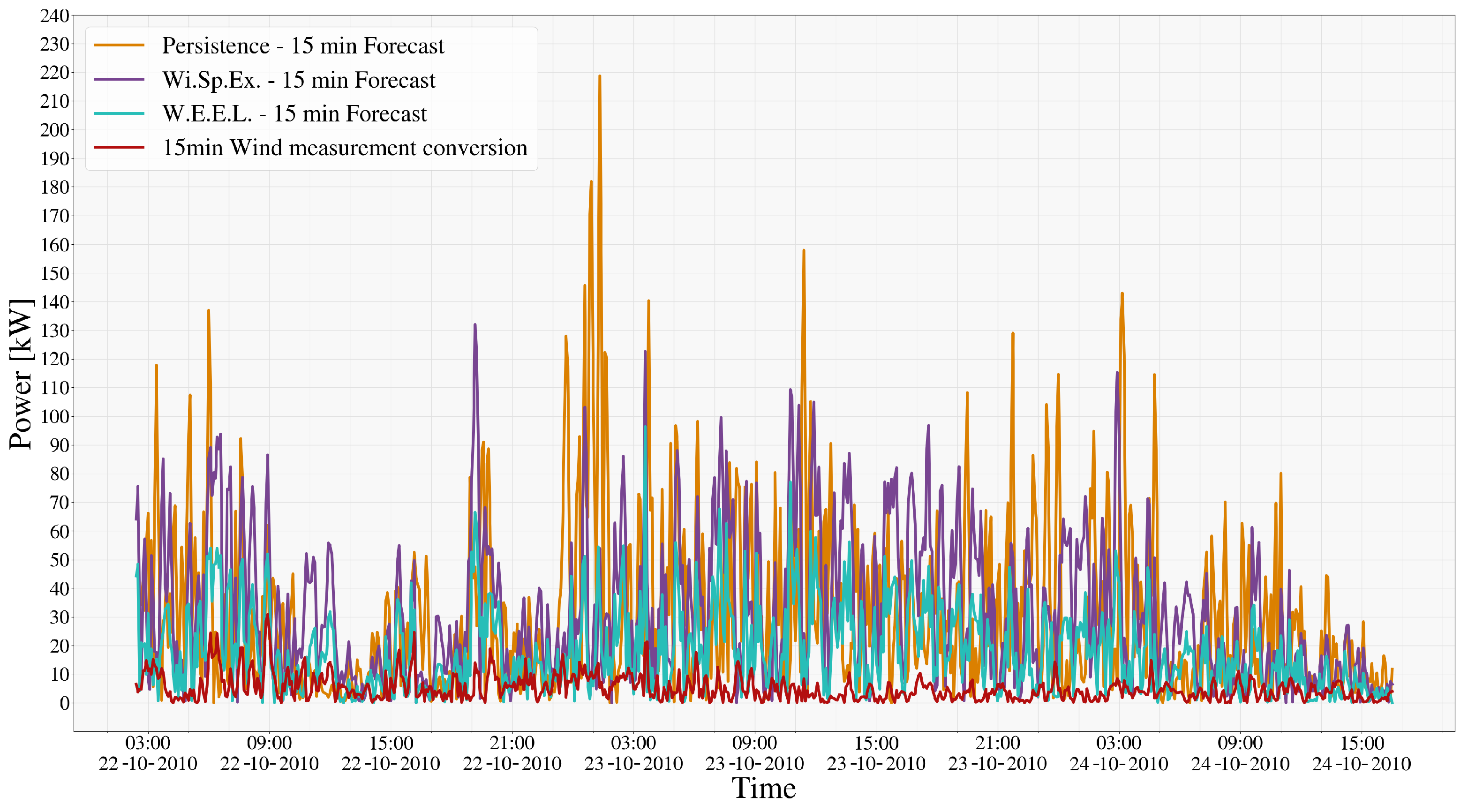
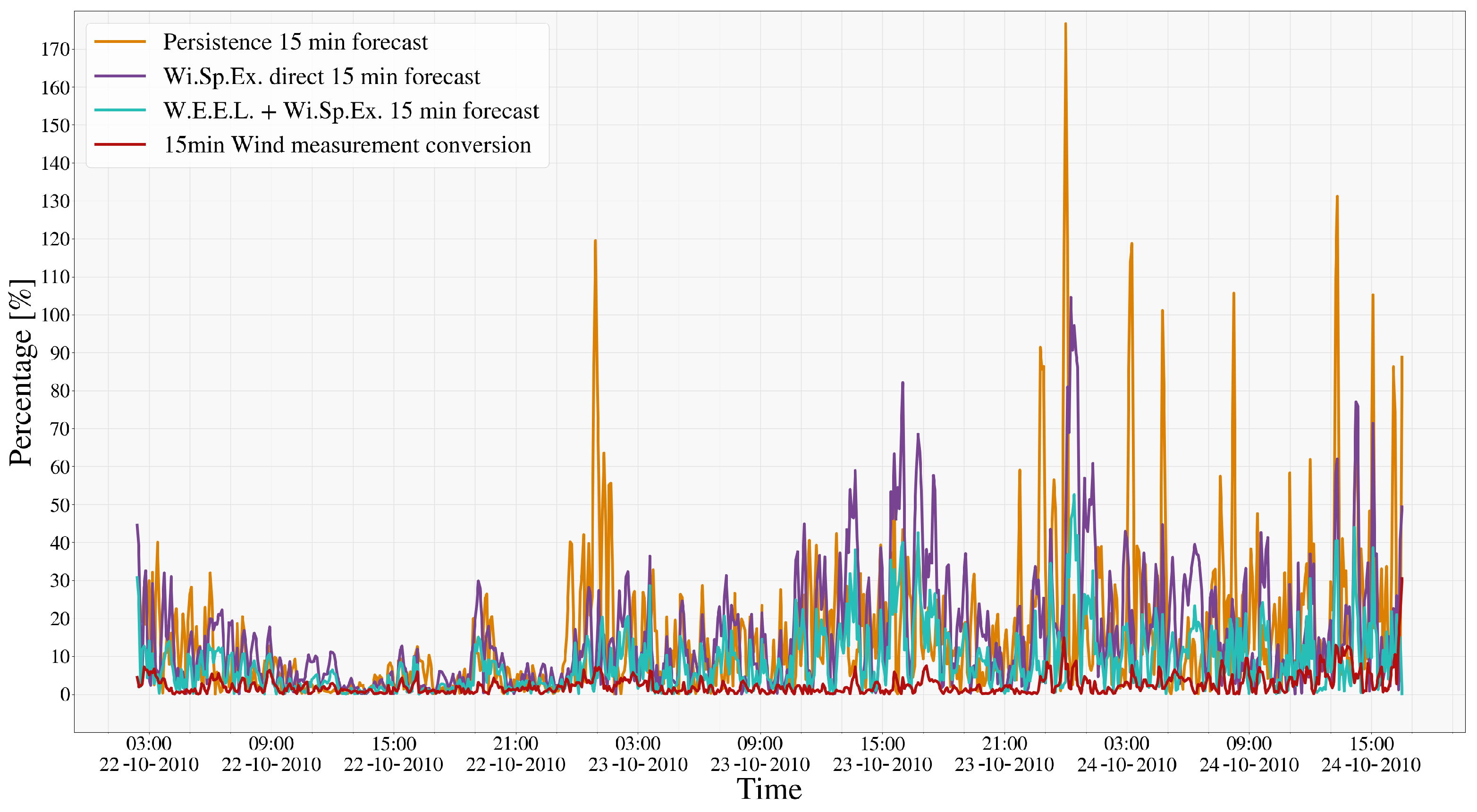
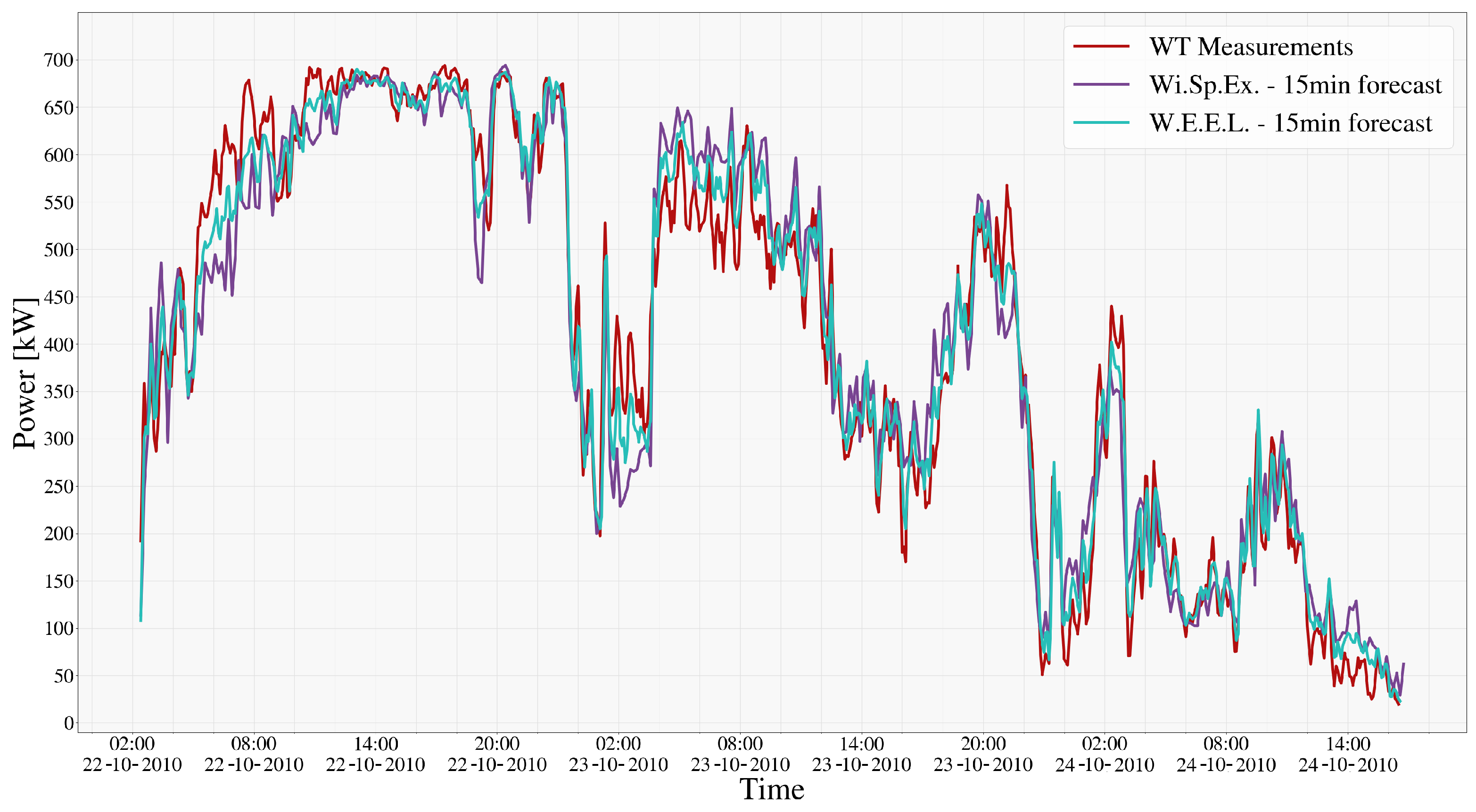
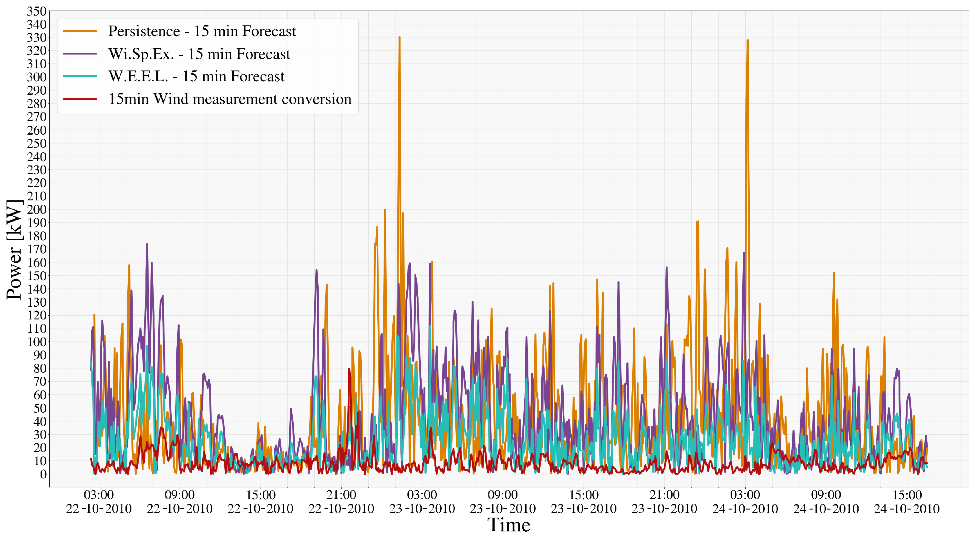
Figure 5 visually depicts the time series of 15 min power forecasts for the Enercon WT, highlighting the performance of WEEL for the first 15 min forecast step in comparison to the direct WiSpEx equivalent forecast (assuming a 10 min phase latency) shifted by the maximum ShiVa. The figure underscores regions where power curve conversion errors tend to be elevated, impacting overall accuracy. Figure 6 illustrates errors inherent to the power curve itself, suggesting potential areas for power curve modeling refinement, particularly at higher wind speeds where power conversion errors tend to escalate. Figure 7 compares errors between WiSpEx and WEEL and persistence.
Further examination reveals that high wind speeds with positive gradients lead to power underestimation, while negative gradients result in overestimation. Low wind speed conditions exhibit more stable behavior with reduced bias. Error variability is significantly influenced by rapid airflow changes, particularly during ramp events. The highest error variance is observed at mid-range wind speeds, likely due to the complex interplay of wind speed magnitude and turbulence. This suggests the potential for further model refinement through the incorporation of advanced power curve modeling techniques and high-quality meteorological data.
Figure 8 and Figure 9 visualize the absolute and absolute percentage errors for WiSpEx and WEEL, respectively, demonstrating the wind speed dependence of power estimation error with decreased error at nominal and low wind speeds. Figure 9 highlights the increased MAPE at lower wind speeds, reflecting the challenges of accurate prediction in low wind energy regimes due to the inherent physical constraints of energy conversion.
Overall, the results highlight WEEL’s capability to provide sufficiently accurate and fast wind power forecasts across various time steps despite the simplifications of the study, contributing to improved grid stability, energy trading efficiency, and the integration of renewable energy sources.

4.2.2. NEG

Table 5 details the performance of the WEEL method in predicting power output for the NEG WT at various time steps. Notably, WEEL exhibits consistently low SMAPE values, all remaining below 10% for all prediction horizons, aligning with Enercon WT results. At the 5 min horizon, WEEL, utilizing a 10 min MA for wind speed, achieves a MAE of 18.48 kW and RMSE of 24.57 kW, while persistence forecasting achieves a MAE of 20.75 kW and RMSE of 29.04 kW. Extending the prediction to 10 min, WEEL with wind power interpolation from adjacent steps maintains its performance (MAE: 18.99 kW, RMSE: 24.73 kW) compared to persistence (MAE: 32.84 kW, RMSE: 46.85 kW). Coupling WEEL with WiSpEx at 15 min horizon further improves upon persistence. At the 15 min horizon, WEEL with WiSpEx achieves a MAE of 24.93 kW and RMSE of 32.24 kW, significantly surpassing persistence (MAE: 42.75 kW, RMSE: 60.3 kW). Persistence MAPE is nearly 77% higher than WEEL’s, and direct WiSpEx forecasts have a 72% higher MAPE, consistent with Enercon WT results.
Figure 10 visually illustrates the 15 min power forecasts for the NEG WT, emphasizing WEEL’s performance at the crucial first 15 min forecast step in comparison to direct WiSpEx forecasts (with a 10 min phase latency) shifted by the maximum ShiVa. Areas of elevated power curve conversion errors are highlighted, impacting overall predictive accuracy.
Figure 11 and Figure 12 provide a detailed error analysis. Figure 11 focuses on power curve-related errors, while Figure 12 compares errors between WiSpEx and WEEL. These figures highlight the potential for model refinement, particularly at higher wind speeds where power conversion errors tend to increase, while Figure 13 and Figure 14 visualize absolute and absolute percentage errors, respectively, showcasing the wind speed dependence of power estimation error and aligning with observations from the Enercon WT analysis.
Similar to the Enercon WT, the NEG WT exhibits a pattern of underestimation at high wind speeds with positive gradients and overestimation with negative gradients. Low wind speed conditions demonstrate more stable behavior. Error variability is significantly influenced by ramp events, with the highest variance observed at mid-range wind speeds.

4.3. Comparative Analysis and Model Performance

The results of the benchmark model presented in this work demonstrate sufficient accuracy (SMAPE < 10%) for a physics-based approach despite the simplifications made to assess its behavior in realistic, non-optimized conditions over complex terrain. This performance highlights its ability to produce results comparable to offline models. This modeling approach is promising not only for its forecasting accuracy but also for its speed, especially considering the simultaneous reconstruction of a wind field from limited measurements. Wi.Sp.Ex. efficiently reconstructs a 3D wind field at 29,928 estimated locations using only nine vertical measurement points per time step, with an average simulation runtime of 104 s (using a maximum of 12 cores of an AMD Ryzen Threadripper 3960X). This runtime can be significantly reduced if high-resolution measurements are available at the inlet of the Wi.Sp.Ex. simulations [5]. WEEL calculations can be performed on a standard laptop. The ShiVa detection calculations are fast, simple, and performed upfront (once), while power conversion can be processed in parallel, ensuring a final runtime below 120 s.
Comparing the two WTs, the Enercon WT consistently demonstrates lower MAPE values than the NEG WT across all forecasting methods. This discrepancy likely stems from variations in power curve selection, WT locations, terrain interactions, and inherent WT characteristics. Both WTs exhibit power estimation errors dependent on wind speed and direction, suggesting potential for further accuracy improvements through correlation methods.
WEEL, coupled with WiSpEx, outperforms persistence forecasting for both WTs, highlighting its ability to model the dynamic nature of wind power generation. Overall, WEEL’s ability to consistently outperform persistence and enhance WiSpEx, along with its robustness in handling various wind conditions, establishes its potential as a valuable tool for accurate and reliable wind power forecasting.
Physics-based models, like the demonstrated WEEL-Wi.Sp.Ex. model, leverage Numerical Weather Prediction (NWP) data and physical principles. They offer interpretability and are valuable when historical data are limited, performing well as short-term (30 min to 24 h ahead) forecasting models, often achieving MAPE values between 5–10% (as in UST forecasting, earlier than 30 min ahead), due to their direct link to measurements and physical understanding. However, their reliance on NWP forecasts can limit their accuracy, especially at longer horizons. Notably, the suggested UST modeling approach achieves comparable accuracy to physics-based models focused on short-term forecasting without relying on NWP output data, leveraging only sparse wind measurements. This underscores the model’s ability to produce forecasts for various time steps and horizons, from minutes to hours ahead, by leveraging advanced measurement techniques and NWP forecasts when available.
Data-driven models leverage historical data to identify patterns and correlations. These models, particularly deep learning architectures, have demonstrated strong performance in capturing wind power dynamics as UST forecasting models. Their adaptability to specific locations is valuable. As demonstrated in [10,11], they can achieve MAPE values in the 3–5% range for the first forecast steps (step size usually ranges from between 5 and 15 min). However, their performance can degrade as they reach the 30 min ahead forecasting horizon, especially when they surpass it (e.g., can reach MAPE > 60% beyond 9 steps in [9,10,11,12]), entering the short-term forecasting region, due to the chaotic nature of wind reducing their accuracy. It is important to recognize that these models typically predict the total power of a WF rather than individual turbines (without providing valuable WT information for operators) like in the suggested modeling approach, and for forecasting horizons greater than 30 min, they may also benefit from incorporating NWP forecasts to enhance accuracy.
The evolution of errors in both model types is noteworthy. Data-driven models usually excel in the immediate future but decline in accuracy over longer horizons. Physics-based models, while slightly less accurate in the immediate future, maintain reasonable performance over longer horizons (more than 30 min ahead). This contrast in error behavior highlights a fundamental trade-off between immediate future precision versus longer horizon stability. The choice of model should therefore be guided by the specific forecasting needs and priorities of the application, considering the relative importance of immediate accuracy versus sustained predictive power. This benchmark model results indicate that physics-based modeling approaches can increase their UST accuracy and speed, naturally improving with the evolution of computational hardware and measurement techniques, ultimately minimizing the implications of such a trade-off.
Ultimately, neither approach is universally superior. Their coexistence and potential integration into hybrid models hold the key to unlocking the full potential of wind power forecasting. This complementary behavior necessitates both approaches in a comprehensive forecasting system. Data-driven models are invaluable for real-time operations, while physics-based models provide longer-term insights and are useful when historical data is scarce.
Hybrid models combining data-driven and physics-based components are increasingly explored [21,22,23,24,41,42,43,44]. They aim to leverage the strengths of both paradigms. The fast modeling approach presented in this work attempts to bridge the scale gap between mesoscale and microscale, particularly in urban areas where NWP resolution is limited. As research progresses, more sophisticated models capable of accurately predicting wind power generation across various timescales can be anticipated, facilitating the seamless integration of this renewable resource into energy systems.

5. Conclusions

The presented model operates under the assumption that the availability of detailed terrain maps that include all major obstacles, which are typically obtained from geographical institutes and public websites to support CFD modeling. Additionally, the assumption that at least one LIDAR system is installed on-site to provide real-time wind data, preferably with a high temporal resolution of one minute or lower is made, a common feature in most modern WT sites. Furthermore, while the wind field is approximated as stationary, this paper demonstrates why this assumption holds under the specific conditions targeted by our model.
This study underscores the potential of physics-based models, exemplified by WEEL coupled with WiSpEx, for enhancing UST wind power forecasting. WEEL’s innovative utilization of MAs, “power lag” identification, and strategic data integration from geographically dispersed measurements contributes to improved forecasting accuracy (WEEL’s MAPE is reduced by more than 40% compared to persistence and direct WiSpEx 15 min-ahead forecasts) and extended prediction horizons, particularly in complex terrains. Validation of this simplified benchmark version of WEEL achieves SMAPE values below 10%, which is extremely promising.
The research highlights the crucial role of CFD-simulated wind speed in forecasting accuracy, emphasizing the impact of wind speed and direction on error behaviour. This is particularly valuable for WFs with limited measurement points, such as the CRES WF. Moreover, in the validation of this benchmark version of WEEL, the use of WiSpEx results as 10 min forecasts and the application of ShiVa detection algorithm, yielded promising results for further extending prediction horizons. Use of high-resolution measurement complex CFD models and state-of-the-art computational hardware are expected to reduce the computational time needed (<2 min) and increase accuracy of the presented modeling approach.
Overall, the use of physics-based models like the one demonstrated in this work as a continuation of [5], presents distinct advantages for UST wind power forecasting. These models offer interpretability, adaptability to diverse environments, and efficacy in scenarios with limited historical data. Notably, WiSpEx reconstructed the 3D wind field over the CRES wind farm using only nine vertical measurement points. This reconstruction, encompassing 29,928 estimated locations, enables wind speed estimation across the entire rotor area rather than relying on a single point at hub height. This capability holds significant promise for future research. WF operators and energy traders can leverage these benefits to improve decision-making, optimize grid integration, and facilitate the seamless incorporation of wind energy into the power system. As research in this field progresses, further advancements in physics-based models, will lead researchers to even more accurate and reliable wind power predictions across various timescales.

Author Contributions

Conceptualization, D.M., F.C. and A.K.; methodology, D.M., F.C. and A.K.; software, D.M.; validation, D.M., F.C. and A.K.; formal analysis, D.M.; investigation, D.M.; resources, A.K. and D.F.; data curation, D.M.; writing—original draft preparation, D.M., F.C. and A.K.; writing—review and editing, D.M., F.C., A.K. and D.F.; visualization, D.M.; supervision, F.C. and A.K.; project administration, F.C. and A.K.; funding acquisition, D.M., F.C. and A.K. All authors have read and agreed to the published version of the manuscript.

Funding

This research has been funded by the Research Committee—University of Patras, under the project “Short-term wind turbine Energy-yield forecasting” (project code: 81023) and co-financed by IMEC.

Data Availability Statement

The datasets presented in this article are not readily available because the data are either part of an ongoing Ph.D. study or belong to CRES. Requests to access the datasets should be directed to the corresponding author.

Acknowledgments

We thank the CRES wind farm for providing us with LIDAR and WT data.

Conflicts of Interest

The authors declare no conflicts of interest. The funders had no role in the design of the study; in the collection, analyses, or interpretation of data; in the writing of the manuscript; or in the decision to publish the results.

Abbreviations

The following abbreviations are used in this manuscript:
CFDComputational Fluid Dynamics
CRESCenter For Renewable Energy Sources
LIDARLight Detection and Ranging
MAMoving Average
MAEMean Absolute Error
MAPEMean Absolute Percentage Error
MSEMean Square Error
NMAENormalized Mean Absolute Error
NRMSENormalized Root Mean Square Error
NWPNumerical Weather Prediction
RMSERoot Mean Square Error
ShiVaShift Value
ShiVaShifted Value
SMAPESymmetric Mean Absolute Percentage Error
SSESum of Squared Errors
USTUltra-Short-Term
WFWind Farm
WiSpExWind Spatial Extrapolation model
WEELWind Energy Extraction Latency model
WTWind Turbine

References

  1. Quiñones, J.J.; Pineda, L.R.; Ostanek, J.; Castillo, L. Towards smart energy management for community microgrids: Leveraging deep learning in probabilistic forecasting of renewable energy sources. Energy Convers. Manag. 2023, 293, 117440. [Google Scholar] [CrossRef]
  2. Manfren, M.; Caputo, P.; Costa, G. Paradigm shift in urban energy systems through distributed generation: Methods and models. Appl. Energy 2011, 88, 1032–1048. [Google Scholar] [CrossRef]
  3. Nallolla, C.A.; P, V.; Chittathuru, D.; Padmanaban, S. Multi-objective optimization algorithms for a hybrid AC/DC microgrid using RES: A comprehensive review. Electronics 2023, 12, 1062. [Google Scholar] [CrossRef]
  4. Polimeni, S.; Nespoli, A.; Leva, S.; Valenti, G.; Manzolini, G. Implementation of different PV forecast approaches in a multiGood microGrid: Modeling and experimental results. Processes 2021, 9, 323. [Google Scholar] [CrossRef]
  5. Michos, D.; Catthoor, F.; Foussekis, D.; Kazantzidis, A. A CFD Model for Spatial Extrapolation of Wind Field over Complex Terrain—Wi. Sp. Ex. Energies 2024, 17, 4139. [Google Scholar] [CrossRef]
  6. Wei, J.; Wu, X.; Yang, T.; Jiao, R. Ultra-short-term forecasting of wind power based on multi-task learning and LSTM. Int. J. Electr. Power Energy Syst. 2023, 149, 109073. [Google Scholar] [CrossRef]
  7. Dai, X.; Liu, G.P.; Hu, W. An online-learning-enabled self-attention-based model for ultra-short-term wind power forecasting. Energy 2023, 272, 127173. [Google Scholar] [CrossRef]
  8. Yang, B.; Zhong, L.; Wang, J.; Shu, H.; Zhang, X.; Yu, T.; Sun, L. State-of-the-art one-stop handbook on wind forecasting technologies: An overview of classifications, methodologies, and analysis. J. Clean. Prod. 2021, 283, 124628. [Google Scholar] [CrossRef]
  9. Xiang, L.; Liu, J.; Yang, X.; Hu, A.; Su, H. Ultra-short term wind power prediction applying a novel model named SATCN-LSTM. Energy Convers. Manag. 2022, 252, 115036. [Google Scholar] [CrossRef]
  10. Liu, L.; Liu, J.; Ye, Y.; Liu, H.; Chen, K.; Li, D.; Dong, X.; Sun, M. Ultra-short-term wind power forecasting based on deep Bayesian model with uncertainty. Renew. Energy 2023, 205, 598–607. [Google Scholar] [CrossRef]
  11. Niu, D.; Sun, L.; Yu, M.; Wang, K. Point and interval forecasting of ultra-short-term wind power based on a data-driven method and hybrid deep learning model. Energy 2022, 254, 124384. [Google Scholar] [CrossRef]
  12. Zhang, Y.; Han, J.; Pan, G.; Xu, Y.; Wang, F. A multi-stage predicting methodology based on data decomposition and error correction for ultra-short-term wind energy prediction. J. Clean. Prod. 2021, 292, 125981. [Google Scholar] [CrossRef]
  13. Sezer-Uzol, N.; Long, L. 3-D time-accurate CFD simulations of wind turbine rotor flow fields. In Proceedings of the 44th AIAA Aerospace Sciences Meeting and Exhibit, Reno, NV, USA, 9–12 January 2006; American Institute of Aeronautics and Astronautics: Reston, VA, USA, 2006; Volume 394. [Google Scholar] [CrossRef]
  14. Wu, Y.T.; Porté-Agel, F. Large-eddy simulation of wind-turbine wakes: Evaluation of turbine parametrisations. Bound.-Layer Meteorol. 2011, 138, 345–366. [Google Scholar] [CrossRef]
  15. Yan, B.; Li, Q. Coupled on-site measurement/CFD based approach for high-resolution wind resource assessment over complex terrains. Energy Convers. Manag. 2016, 117, 351–366. [Google Scholar] [CrossRef]
  16. Yan, S.; Shi, S.; Chen, X.; Wang, X.; Mao, L.; Liu, X. Numerical simulations of flow interactions between steep hill terrain and large scale wind turbine. Energy 2018, 151, 740–747. [Google Scholar] [CrossRef]
  17. Valldecabres, L.; Peña, A.; Courtney, M.; von Bremen, L.; Kühn, M. Very short-term forecast of near-coastal flow using scanning lidars. Wind Energy Sci. 2018, 3, 313–327. [Google Scholar] [CrossRef]
  18. Kajishima, T.; Taira, K. Computational Fluid Dynamics: Incompressible Turbulent Flows; Springer: Cham, Switzerland, 2016. [Google Scholar] [CrossRef]
  19. Ferziger, J.H.; Perić, M. Computational Methods for Fluid Dynamics, 4th ed.; Springer: Cham, Switzerland, 2020. [Google Scholar] [CrossRef]
  20. Wendt, J. Computational Fluid Dynamics: An Introduction; A von Karman Institute Book; Springer: Berlin/Heidelberg, Germany, 2008. [Google Scholar] [CrossRef]
  21. Chen, N.; Qian, Z.; Nabney, I.T.; Meng, X. Wind Power Forecasts Using Gaussian Processes and Numerical Weather Prediction. IEEE Trans. Power Syst. 2014, 29, 656–665. [Google Scholar] [CrossRef]
  22. Du, P. Ensemble machine learning-based wind forecasting to combine NWP output with data from weather stations. In Renewable Energy Integration for Bulk Power Systems: ERCOT and the Texas Interconnection; Springer International Publishing: Cham, Switzerland, 2023; pp. 263–281. [Google Scholar] [CrossRef]
  23. Shirzadi, N.; Nasiri, F.; Menon, R.P.; Monsalvete, P.; Kaifel, A.; Eicker, U. Smart Urban Wind Power Forecasting: Integrating Weibull Distribution, Recurrent Neural Networks, and Numerical Weather Prediction. Energies 2023, 16, 6208. [Google Scholar] [CrossRef]
  24. Chang, Y.; Yang, H.; Chen, Y.; Zhou, M.; Yang, H.; Wang, Y.; Zhang, Y. A Hybrid Model for Long-Term Wind Power Forecasting Utilizing NWP Subsequence Correction and Multi-Scale Deep Learning Regression Methods. IEEE Trans. Sustain. Energy 2024, 15, 263–275. [Google Scholar] [CrossRef]
  25. Zhou, L.; Hu, G.; Tse, K.T.; He, X. Twisted-wind effect on the flow field of tall building. J. Wind Eng. Ind. Aerodyn. 2021, 218, 104778. [Google Scholar] [CrossRef]
  26. Xiaoxia, G.; Luqing, L.; Shaohai, Z.; Xiaoxun, Z.; Haiying, S.; Hongxing, Y.; Yu, W.; Hao, L. LiDAR-based observation and derivation of large-scale wind turbine’s wake expansion model downstream of a hill. Energy 2022, 259, 125051. [Google Scholar] [CrossRef]
  27. Wilcox, D.C. Turbulence Modeling for CFD, 3rd ed.; DCW Industries, Inc.: La Cañada, CA, USA, 2006. [Google Scholar]
  28. Emeis, S. Wind Energy Meteorology: Atmospheric Physics for Wind Power Generation; Springer: Berlin/Heidelberg, Germany, 2018. [Google Scholar] [CrossRef]
  29. Choukulkar, A.; Pichugina, Y.; Clack, C.T.; Calhoun, R.; Banta, R.; Brewer, A.; Hardesty, M. A new formulation for rotor equivalent wind speed for wind resource assessment and wind power forecasting. Wind Energy 2016, 19, 1439–1452. [Google Scholar] [CrossRef]
  30. Shourangiz-Haghighi, A.; Haghnegahdar, M.A.; Wang, L.; Mussetta, M.; Kolios, A.; Lander, M. State of the art in the optimisation of wind turbine performance using CFD. Arch. Comput. Methods Eng. 2020, 27, 413–431. [Google Scholar] [CrossRef]
  31. COMSOL Multiphysics® (CFD). COMSOL Multiphysics® CFD Module User’s Guide, Version 5.6; COMSOL: Burlington, MA, USA, 2020. [Google Scholar]
  32. COMSOL Multiphysics® (CYCLOPEDIA). COMSOL Multiphysics® CYCLOPEDIA; COMSOL: Burlington, MA, USA, 2017. [Google Scholar]
  33. COMSOL Multiphysics® (Reference Manual). COMSOL Multiphysics® Reference Manual, Version 5.6; COMSOL: Burlington, MA, USA, 2020. [Google Scholar]
  34. Tavner, P.; Edwards, C.; Brinkman, A.; Spinato, F. Influence of wind speed on wind turbine reliability. Wind Eng. 2006, 30, 55–72. [Google Scholar] [CrossRef]
  35. Morren, J.; Pierik, J.; De Haan, S.W. Inertial response of variable speed wind turbines. Electr. Power Syst. Res. 2006, 76, 980–987. [Google Scholar] [CrossRef]
  36. Hassan, A.; Rehman, A.U.; Shabbir, N.; Hassan, S.R.; Sadiq, M.T.; Arshad, J. Impact of inertial response for the variable speed wind turbine. In Proceedings of the IEEE 2019 International Conference on Engineering and Emerging Technologies (ICEET), Lahore, Pakistan, 21–22 February 2019; pp. 1–6. [Google Scholar] [CrossRef]
  37. Virtanen, P.; Gommers, R.; Oliphant, T.E.; Haberland, M.; Reddy, T.; Cournapeau, D.; Burovski, E.; Peterson, P.; Weckesser, W.; Bright, J.; et al. SciPy 1.0: Fundamental algorithms for scientific computing in Python. Nat. Methods 2020, 17, 261–272. [Google Scholar] [CrossRef]
  38. Saint-Drenan, Y.M.; Besseau, R.; Jansen, M.; Staffell, I.; Troccoli, A.; Dubus, L.; Schmidt, J.; Gruber, K.; Simões, S.G.; Heier, S. A parametric model for wind turbine power curves incorporating environmental conditions. Renew. Energy 2020, 157, 754–768. [Google Scholar] [CrossRef]
  39. Bingöl, F.; Mann, J.; Foussekis, D. 2.3 Lidar in complex terrain. In Advancements in Wind Energy Metrology—UPWIND 1A2.3; Danmarks Tekniske Universitet: Copenhagen, Denmark, 2011; p. 11. [Google Scholar]
  40. CRES. Technical Specs of the WTs; CRES: Kansas City, MI, USA, 2024. [Google Scholar]
  41. He, B.; Ye, L.; Pei, M.; Lu, P.; Dai, B.; Li, Z.; Wang, K. A combined model for short-term wind power forecasting based on the analysis of numerical weather prediction data. Energy Rep. 2022, 8, 929–939. [Google Scholar] [CrossRef]
  42. Yang, M.; Wang, D.; Zhang, W. A short-term wind power prediction method based on dynamic and static feature fusion mining. Energy 2023, 280, 128226. [Google Scholar] [CrossRef]
  43. Yakoub, G.; Mathew, S.; Leal, J. Intelligent estimation of wind farm performance with direct and indirect ‘point’ forecasting approaches integrating several NWP models. Energy 2023, 263, 125893. [Google Scholar] [CrossRef]
  44. Liu, C.; Zhang, X.; Mei, S.; Zhou, Q.; Fan, H. Series-wise attention network for wind power forecasting considering temporal lag of numerical weather prediction. Appl. Energy 2023, 336, 120815. [Google Scholar] [CrossRef]
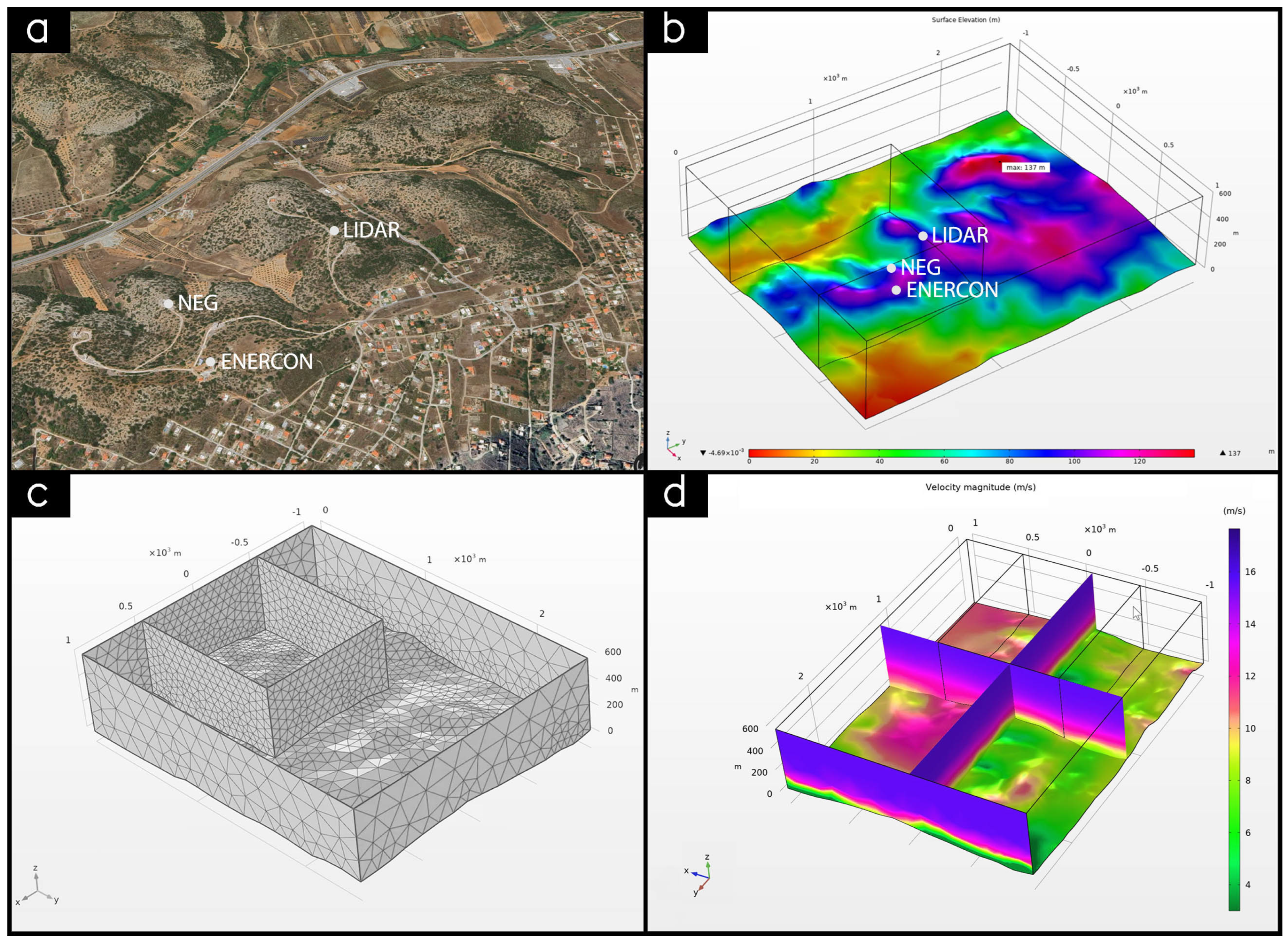
Figure 1. (a) Map showing the location of the CRES WF and the LIDAR and WT measurement locations in Lavrio, Greece. (b) Elevation map of the terrain surrounding the CRES WF used in the Wi.Sp.Ex. simulations. (c) Mesh used for the CFD simulations of the CRES WF in Wi.Sp.Ex. (d) Wind speed prediction results from the Wi.Sp.Ex. simulation.
Energies 17 05493 g001
Figure 2. WEEL diagram.
Energies 17 05493 g002
Figure 3. Enercon—Optimal and Maximum ShiVA Detection scatter plots. (a) No shift; (b) Optimal ShiVA shift (+3 min); (c) Maximum ShiVA shift (+5 min).
Energies 17 05493 g003aEnergies 17 05493 g003b
Figure 4. NEG—optimal and maximum ShiVA detection scatter plots. (a) No shift; (b) Optimal ShiVA shift (+3 min); (c) Maximum ShiVA shift (+5 min).
Energies 17 05493 g004
Figure 5. Time series of 15 min power forecasts for the Enercon WT.
Energies 17 05493 g005
Figure 6. Errors in 15 min power conversion from measured wind speed for the Enercon WT.
Energies 17 05493 g006
Figure 7. Comparison of 15 min power forecast errors between WiSpEx and WEEL and persistence for the Enercon WT.
Energies 17 05493 g007
Figure 8. Absolute errors of power forecasts for the Enercon WT.
Energies 17 05493 g008
Figure 9. Absolute percentage errors of power forecasts for the Enercon WT.
Energies 17 05493 g009
Figure 10. Time series of 15 min power forecasts for the NEG WT.
Energies 17 05493 g010
Figure 11. Errors in 15 min power conversion from measured wind speed for the NEG WT.
Energies 17 05493 g011
Figure 12. Comparison of 15 min power forecast errors between WiSpEx and WEEL and persistence for the NEG WT.
Energies 17 05493 g012
Figure 13. Absolute errors of power forecasts for the NEG WT.
Energies 17 05493 g013
Figure 14. Absolute percentage errors of power forecasts for the NEG WT.
Energies 17 05493 g014
Table 1. Characteristics of Enercon E40-500 and NEG NM 750/48 WTs, part of table presented in [40].
SpecificationE40-500NM 750/48
RotorDiameter40 m48.2 m
Area swept1275 m21824 m2
Number of blades33
TypeUpwind rotor with active pitch controlUpwind Rotor
TowerHub height (approx.)44 m45 m
GeneratorTypeDirect-driven ENERCON ring generator (with drive train)Asynchronous, 4/6 pole
Name plate rating500 kW750/200 kW
Nominal Voltage500 V690 V
Nominal Frequency50 Hz50 Hz
Operational DataNominal output500 kW750 kW
Cut-in wind speed2.5 m/s4 m/s
Nominal wind speed12 m/s16 m/s
Power regulationVariable Speed + PitchStall
Table 2. WEEL—Enercon shift stats.
Metric+0 min Shift+1 min Shift+2 min Shift+3 min Shift+4 min Shift+5 min Shift
MAE12.96111.57710.83810.67511.12912.353
MSE293.660231.483204.463201.226220.992274.580
RMSE17.13615.21414.29914.18514.86516.570
MAPE6.3425.6645.3175.2255.4165.988
Table 3. WEEL—NEG shift stats.
Metric+0 min Shift+1 min Shift+2 min Shift+3 min Shift+4 min Shift+5 min Shift
MAE18.38516.93016.38416.49017.17918.653
MSE614.732511.373470.061472.260518.871629.909
RMSE24.79322.61321.68021.73122.77825.097
MAPE7.5616.8726.6016.6526.9887.74
Table 4. Enercon 15 min power forecast errors stats for various forecast methods and time steps.
Method15 min MAWEEL (Direct)Persistence Power InterpolatedWEELPersistenceWEEL (Wi.Sp.Ex.)Wi.Sp.Ex.Persistence
MAE [kW]5.0612.2315.3212.9624.8517.8131.5831.82
MSE [kW2]45.18271.15450.05294.811188.44532.481643.361938.99
RMSE [kW]6.7216.4721.2117.1734.4723.0840.5444.03
MAPE [%]2.45.917.416.112.28.4415.3616.01
NMAE0.01010.02450.03060.02590.04970.03560.06320.0636
NRMSE0.01340.03300.04240.03430.06900.04620.08110.0881
SMAPE [%]2.395.887.295.9911.728.1814.5115.03
time steplive+5 min+5 min+10 min+10 min+15 min+15 min+15 min
Table 5. NEG 15 min power forecast errors stats for various forecast methods and time steps.
Method15 min MAWEEL (Direct)PersistenceWEEL Power InterpolatedPersistenceWEEL (Wi.Sp.Ex.)Wi.Sp.Ex.Persistence
MAE [kW]8.1518.4820.7518.9932.8424.9343.1942.75
MSE [kW2]121.24603.92843.16611.472195.321039.33176.673635.62
RMSE [kW]11.0124.5729.0424.7346.8532.2456.3660.3
MAPE [%]3.867.678.217.9513.6510.2517.7118.14
NMAE0.01090.02460.02770.02530.04380.03320.05760.0570
NRMSE0.01480.03280.03870.03290.06260.04300.07510.0804
SMAPE [%]3.717.538.07.4412.689.2615.2816.12
time steplive+5 min+5 min+10 min+10 min+15 min+15 min+15 min
Disclaimer/Publisher’s Note: The statements, opinions and data contained in all publications are solely those of the individual author(s) and contributor(s) and not of MDPI and/or the editor(s). MDPI and/or the editor(s) disclaim responsibility for any injury to people or property resulting from any ideas, methods, instructions or products referred to in the content.