Article

A Fusion Model for Predicting the Vibration Trends of Hydropower Units

1
China Yangtze Power Co., Ltd., Wuhan 430014, China
2
Hubei Technology Innovation Center for Smart Hydropower, Wuhan 430019, China
3
Hubei Provincial Key Laboratory of Design and Maintenance of Hydropower Machinery, China Three Gorges University, Yichang 443002, China
*
Author to whom correspondence should be addressed.
Energies 2024, 17(23), 5847; https://doi.org/10.3390/en17235847
Submission received: 19 October 2024 / Revised: 11 November 2024 / Accepted: 13 November 2024 / Published: 22 November 2024

Abstract

:
Hydropower units are essential to the safe, stable, and efficient operation of modern power systems, particularly given the current expansion of renewable energy systems. To enable timely monitoring of unit performance, it is critical to investigate the trends in vibration signals, to enhance the accuracy and reliability of vibration trend prediction models. This paper proposes a fusion model for the vibration signal trend prediction of hydropower units based on the waveform extension method empirical mode decomposition (W-EMD) and long short-term memory neural network (LSTMNN). The fusion model first employed a waveform matching extension method based on parameter ergodic optimization to extend the original signal. Secondly, EMD was used to decompose the extended signal sequence and reconstruct the decomposition components by the extreme point division method, and the reconstructed high- and low-frequency components were used as LSTMNN inputs for component prediction. Finally, the component prediction results were superimposed with equal weights to obtain the predicted value of the vibration signal trend of the hydropower unit. The experimental results showed that the W-EMD signal decomposition method can effectively suppress the endpoint effect problem in the traditional EMD algorithm, improving the quality of EMD decomposition. Furthermore, through a case study of the upper guide X direction swing signal on the 16F unit of a domestic hydropower station, it was found that the proposed fusion model successfully predicted anomalies in the unit’s swing signals; compared with SVR, KELM, LSTMNN, and EMD + LSTMNN, the prediction accuracy was improved by 78.94%, 66.67%, 55.56%, and 42.86%, respectively.

1. Introduction

In the new power system, hydropower energy as a ‘stabilizer’ for the safe operation of the system plays a crucial role, and the core equipment of hydropower is the hydropower unit [1,2]. In the actual production process, the hydropower unit, as an important equipment for grid peak shifting and frequency regulation, is affected by hydraulic, mechanical, electrical, and other comprehensive factors in the operation process, so that the hydropower unit produces a variety of faults and hidden dangers, which seriously affects the operational status of hydropower plants [3,4,5]. With the continuous changes in operating conditions and the accumulation of operating time, the performance of the unit equipment deteriorates continuously, and even serious failures occur, increasing the maintenance cost of the unit. The vibration and swing signals of a hydropower unit are a key monitoring quantity to characterize its stable operation and contain a large amount of information on the operating status of the equipment [6,7]. Therefore, research on the trend of vibration and oscillation signals of the unit can timely grasp its operating status and law, avoid potential equipment failure risks, and thus effectively improve the comprehensive benefits of hydropower stations [8,9].
The key to predicting the vibration and swing trend of a hydropower unit is to obtain vibration and swing monitoring data on its key components during unit operation [10]. Due to the non-smoothness and non-linearity of the vibration and swing signals, researchers apply the empirical mode decomposition (EMD) [11] algorithm to the vibration and swing signals of the unit and use the signal decomposition algorithm to preprocess the oscillation data of the unit in order to get smoother sequence data and fully extract the information on the unit’s operation state. In the EMD process, there is sometimes an inability to clearly judge the extreme values at the endpoints, which in turn produces a ‘flying wing’ phenomenon when fitting the envelope at the endpoints [12,13]. Aiming at the endpoint effect problem in EMD of short data sequences, scholars at home and abroad have undertaken a considerable amount of research, and the main solutions include two categories: one is to improve the algorithm itself [14,15,16]; the other is to preprocess the signal itself [12,17,18]. Long short-term memory neural network (LSTMNN) as an improved variant of temporal recurrent neural networks has been widely used in deep learning fields such as time series prediction because of its characteristics of solving problems such as gradient explosion and gradient vanishing [19,20,21,22].
In order to improve the accuracy of trend prediction and reduce the influence of non-linear and non-stationary signals of the unit on the prediction results, combining signal decomposition algorithms with machine learning prediction models [9,23,24] has become the focus of trend prediction research. Hu et al. [25] adopted a noise reduction method combining BA-VMD and wavelet thresholding and a long short-term memory network (LSTM) prediction model to predict the trend of vibration signals. Qin et al. [26] established a long short-term memory neural network (LSTM) prediction model for wind speed prediction on the original wind speed series. Wang et al. [27] introduced a long short-term memory (LSTM) neural network and proposed a comprehensive deterioration index (CDI) trend prediction model based on the time–frequency domain, improving the prediction accuracy for the condition trend of hydropower units. Zhao et al. [28] proposed a prediction technique for short-term traffic flow, which utilizes empirical modal decomposition (EMD) and long short-term memory neural networks (LSTM). Based on this, this paper proposes a trend prediction fusion model for hydropower unit vibration and swing signals based on W-EMD and LSTMNN. The fusion model first employed a waveform matching extension method based on parameter ergodic optimization to extend the original signal. Secondly, EMD was used to decompose the extended signal sequence and reconstruct the decomposition components by the extreme point division method, and the reconstructed high- and low-frequency components were used as LSTMNN inputs for component prediction. Finally, the component prediction results were superimposed with equal weights to obtain the predicted value of the vibration signal trend of the hydropower unit. Taking the upper guide X direction swing signal of a hydropower unit as an example, the effectiveness of the fusion model in the oscillation trend prediction of the unit was verified.
In summary, the main contribution of this paper can be summarized as follows:
  • An EMD endpoint effect suppression method based on waveform matching extended (W-EMD) is proposed.
  • Combining the proposed endpoint effect suppression method with LSTMNN and reconstructing the decomposed signal by the method of extreme point division greatly improves the quality of signal decomposition as well as the prediction accuracy of the algorithmic model.
  • The validity of the proposed method for predicting the vibration trend of hydropower units is demonstrated through validation tests on specific examples.
The remainder of this paper is structured as follows: Section 2 describes in detail the process of constructing the W-EMD + LSTMNN model and explains the individual evaluation metrics. Section 3 proposes a concrete implementation of the Waveform matching extension-based EMD endpoint effect suppression approach. Section 4 verifies the validity and superiority of the proposed model with a specific example of the swing of the upper guide X direction of the hydropower unit, and the test results are analyzed in detail. Finally, Section 5 summarizes the entire paper.

2. Model Construction and Related Evaluation Indicators

2.1. Establishment of Vibration and Swing Signals Trend Prediction Model for Hydropower Units

The proposed hydropower unit oscillation trend prediction model takes the upper guide swing signal as an example, and first uses the parameter traversal optimization waveform matching extension method to extend the signal endpoints in order to inhibit the endpoint effect generated by EMD. Secondly, the EMD algorithm is used to decompose the extended data to obtain multiple eigenmode components and residual components, and the eigenmode components obtained from the decomposition are reconstructed by using the method of polar point division, i.e., all the components are divided into the high-frequency component (HFC) and the low-frequency component (LFC) by calculating the number of polar points contained in each component. Finally, LSTMNN is used to predict the high- and low-frequency component signals of the up-conducted swing signal of the hydropower unit, and the component prediction results are superimposed with equal weights to obtain the final prediction of the up-conducted swing. The signal component obtained by this method significantly reduces the amount of prediction calculation and the complexity of the prediction model and effectively improves the model prediction efficiency, prediction stability, and generalization ability. A flowchart of the prediction model construction is shown in Figure 1.

2.2. Evaluation Indicators for Endpoint Effects

For an assessment of the effect of suppressing the endpoint effect, qualitative evaluation indexes need to be selected, and in this paper, the similarity coefficients between the EMD component signals and the actual components of the corresponding original signals are used to assess the effect of suppressing the endpoint effect. The formula for calculating the similarity coefficient is as follows [29]:
ρ ( x i ( t ) , i m f i ( t ) ) = cov ( x i ( t ) , i m f i ( t ) ) σ ( x i ) σ ( i m f i )
where cov ( ) denotes the covariance; σ ( ) is the variance; imfi denotes the i-th eigenmode component of the signal after EMD; and xi is the actual constituent component of the corresponding original signal. The larger the value of the similarity coefficient, the better the suppression of the endpoint effect.

2.3. Predictive Model Evaluation Indicators

In order to compare more intuitively the prediction effect of the constructed fusion prediction model on the trend of the vibration and swing signals of the hydropower unit, mean absolute error (MAE), mean absolute percentage error (MAPE), mean square error (MSE), and mean square percentage error (MSPE) are used as the evaluation indexes of the prediction effect of the vibration and swing signals. The calculation formula is as follows [30,31]:
M A E = 1 N i = 1 N y i ^ y i
M A P E = 1 N i = 1 N y i ^ y i y i
M S E = 1 N i = 1 N y i ^ y i 2
M S P E = 1 N i = 1 N y i ^ y i y i 2
where y i is the actual value of the X direction swing in the upper guide of the hydropower unit, and y i ^ is the predicted value of the X direction swing in the upper guide.

3. Improvement of EMD Algorithm

In order to adopt a suitable method for endpoint effect suppression, this study proposes a waveform-matching extended method based on parameter traversal optimization to improve the quality of empirical modal decomposition based on the pre-processing method of the signal itself.

3.1. Waveform Matching Extended Method Based on Parameter Traversal Optimization

3.1.1. Definition of Waveform Matching Related Parameters

In this study, the signal waveform matching degree is defined by considering the similarity of signals in shape and amplitude. The Pearson correlation coefficient reflects the degree of linear correlation between two variables, i.e., the degree of similarity in shape between the characteristic waveform and the matched waveform, and is calculated as follows [32]:
ρ ( x , y ) = cov ( x , y ) σ ( x ) σ ( y )
where cov ( ) is the covariance between the two variables, and σ ( ) is the variance between the variables. The closer the correlation coefficient is to 1 or −1, the stronger the correlation between the variables; the closer it is to 0 the weaker the linear correlation between the variables.
The Euclidean distance is used to measure the similarity in amplitude between the eigenwave and the matching wave, and the formula is as follows [33]:
d ( x , y ) = ( ( x i y i ) 2 )
The Euclidean distance is usually expressed using the Euclidean distance similarity s [34]:
s = 1 1 + d ( x , y )
where the value of s is in the range of [0, 1], and the larger the distance similarity s is, the smaller d is, i.e., the closer the distance is, the larger the similarity is.
Finally, the above shape similarity and amplitude similarity index parameters are reasonably integrated to obtain a comprehensive index for evaluating the matching degree of waveforms, in order to comprehensively consider the degree of similarity between the characteristic waveforms and the matched waveforms. Collating Equations (6)–(8) yields a composite metric for waveform matching as:
P = α × ρ + ( 1 α ) × s , α [ 0 , 1 ]
where α is the degree of match parameter.

3.1.2. Verification of Simulated Signals

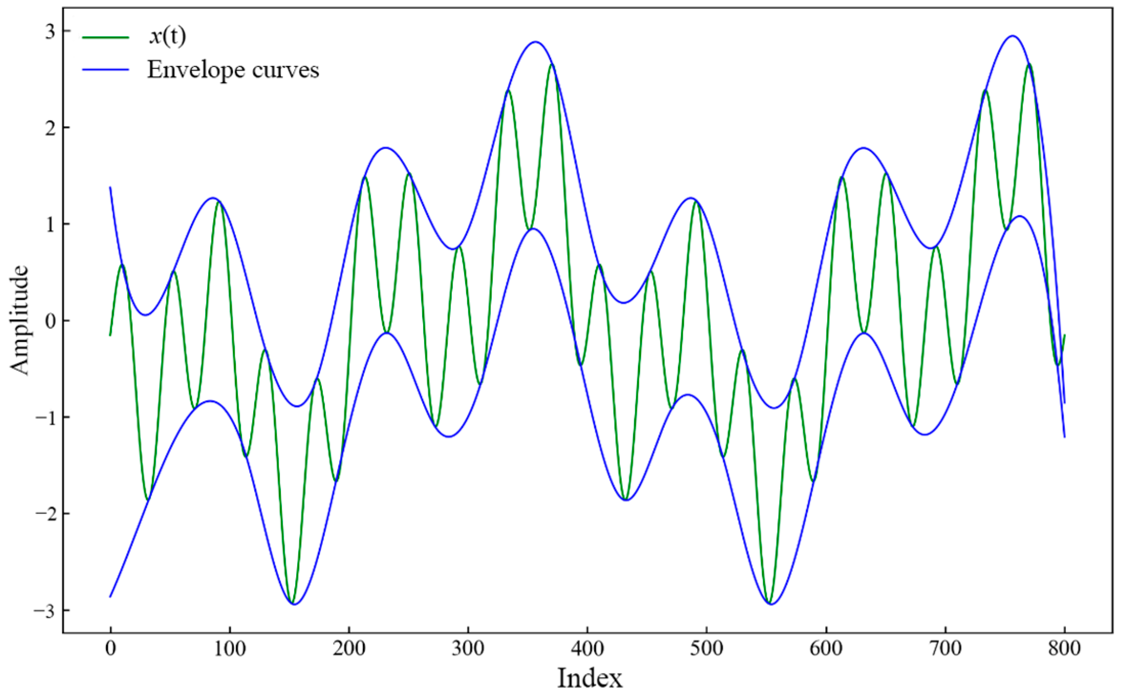
Taking the simulated signal x(t) as an example, the sampling frequency of the signal is 600 Hz and the number of sampling points is 800.
x ( t ) = cos ( 2 π × 2 t + 1 ) + sin ( 2 π × 20 t + 6 ) + cos ( 2 π × 6 t + 2 )
From Figure 2, the simulated signal fitted by cubic spline interpolation produces the phenomenon of endpoint ‘flying wing’ due to the inability to determine the extreme values at the endpoints.
The waveform matching extended-based method is used to suppress the endpoint effect of the signal during EMD. The specific steps of the method are:
(1)
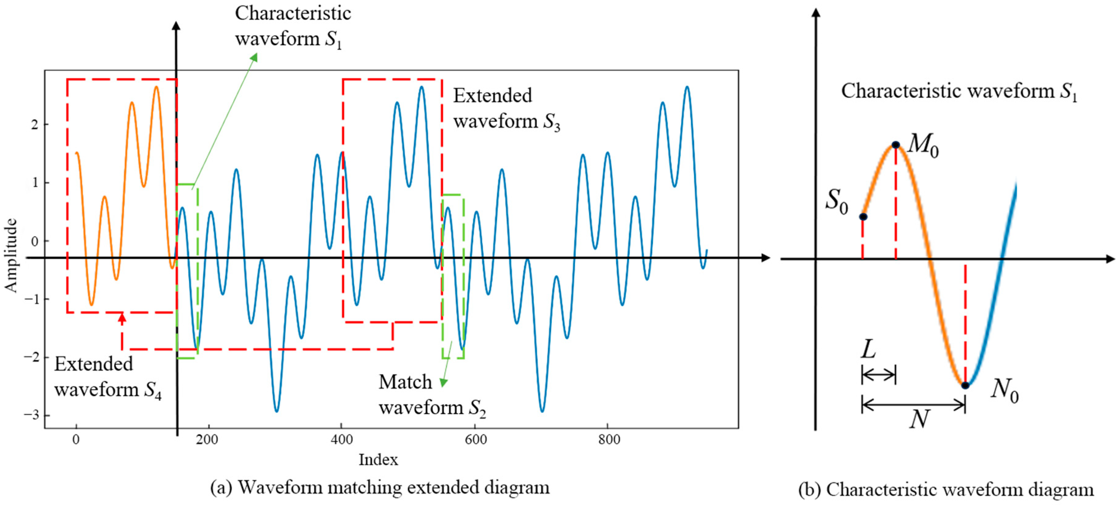
Taking the extended extension of the left endpoint of the simulated signal x(t) as an example, the characteristic wave S1 (shown in Figure 3b) is defined, which has a very large value point followed by a very small value point. Denote the left endpoint corresponding to the eigenwave as S0, the first extreme value point as M0, and the first minimal value point as N0; the length of the eigenwave is N, and the distance between the left endpoint S0 and the first extreme value point M0 is L. For practical analysis, the characteristic wavelength can be defined according to the measured signal characteristics.
(2)
Mark the extremely large and extremely small points within the index range of the simulated signal x(t), and denote the set consisting of all extremely large points as Mmax and the set consisting of all extremely small points as Mmin. Set the initial value of the waveform match parameter α and the traversal step, take the first maximal point M0 as a reference point, such that the length of the matching wave is the same as the length of the eigenwave, and calculate the composite index of waveform matching P for different values of the matching parameter α .
(3)
The signal before the maximum value of the waveform matching index Pmax corresponding to the matching wave is used as the extended wave to extend the original signal. Record that the coordinate of the extreme value corresponding to M0 at this point is Mp, and the coordinate corresponding to S0 is Xp = Mp- − L.
(4)
Set in advance the number of points to be extended n, and using the waveform corresponding to the first n points of Xp as the extended wave S3, the extension of the left end of the signal x(t) is completed by moving this extended wave to just before S0. Figure 3a shows the schematic diagram of the left endpoint of the simulated signal after it is extended. Similarly, an extended extension of the right end of the simulated signal can be achieved.
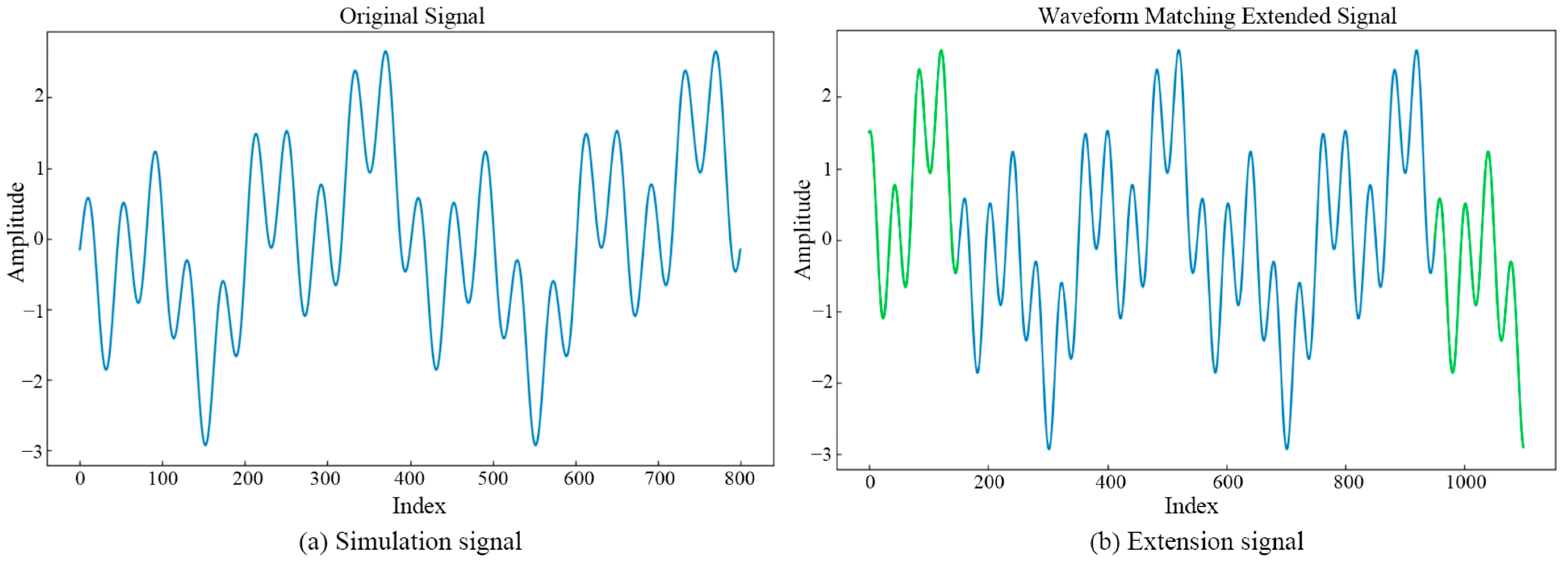
The x(t) extended results obtained by the above steps are shown in Figure 4.
In order to verify the effectiveness of the waveform matching extended method proposed in this paper, the empirical modal decomposition of the simulated signal x(t) and its extended signal is carried out. Setting the number of signal left and right endpoint extended points as n = 150, the actual component time sampling points range from 150 to 950 after they are extended, and the decomposition results are shown in Figure 5. Figure 5a shows the result of the decomposition of the simulated signal x(t); the green dashed line is the actual component of the signal and the red solid line is the EMD component, and it is clearly observed that there is a fitting error at the endpoints of the components. Figure 5b shows the result of the decomposition of the signal after it is extended, and the EMD components are highly coincident with the actual components of the signal. According to Equation (1), the results of the comparison of similarity coefficients of each component before and after the signal is extended are shown in Table 1. As can be seen from Table 1, the EMD endpoint effect of the simulated signal x(t) is significantly improved after it is extended by the parameter traversal optimization waveform matching extension method, which verifies the effectiveness of the extension method in suppressing the EMD endpoint effect.

4. Instance Validation

4.1. Trend Prediction Analysis of Upper Guide Swing Signal on Hydropower Units

In order to verify the prediction effect of the proposed W-EMD and LSTMNN fusion model, an experimental study and validation were conducted for the monitoring data of unit 16F of a hydropower station in China. Taking the X direction swing signal of the upper guide in the unit from 1 January 2023–30 July 2023 as the research object, the trend plot of the upper guide X direction swing after outlier removal and missing value processing is shown in Figure 6a. During the period from 1 January–16 July, the unit was in a stable operation state, but on 17 July 2023, the upper guide slip rotor of the unit suddenly went up, causing the upper guide swing to trigger a large alarm. In order to better strengthen the role of near-term data and weaken the impact of forward data, the above-mentioned cleaned upper guide swing data is processed by sliding average to remove the jump value of the original data and improve the data quality. The sliding window size is set to window_size = 50, and the processed upper guide X direction swing signal is shown in Figure 6b.

4.2. Swing Signal Decomposition and Component Reconstruction

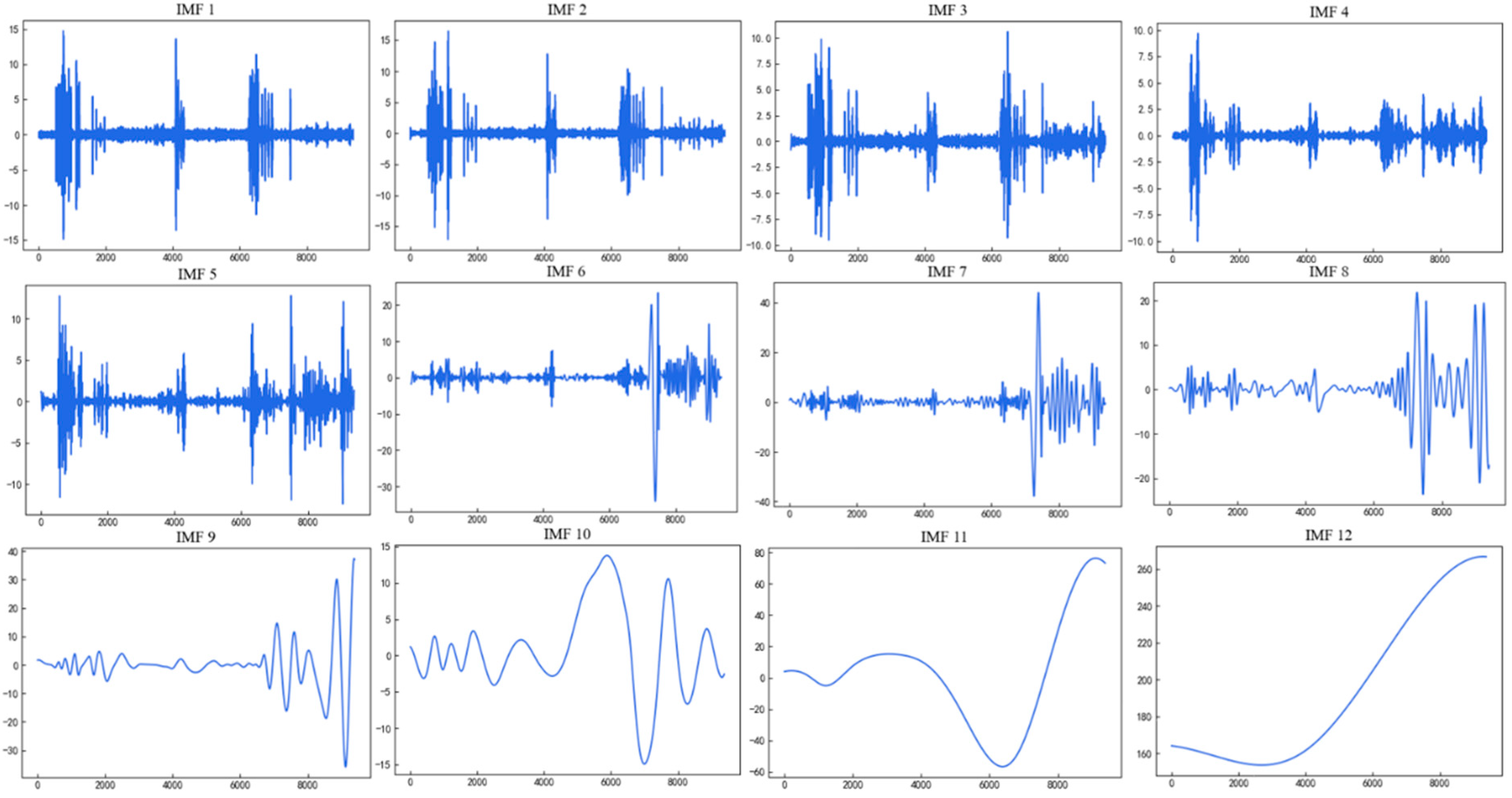
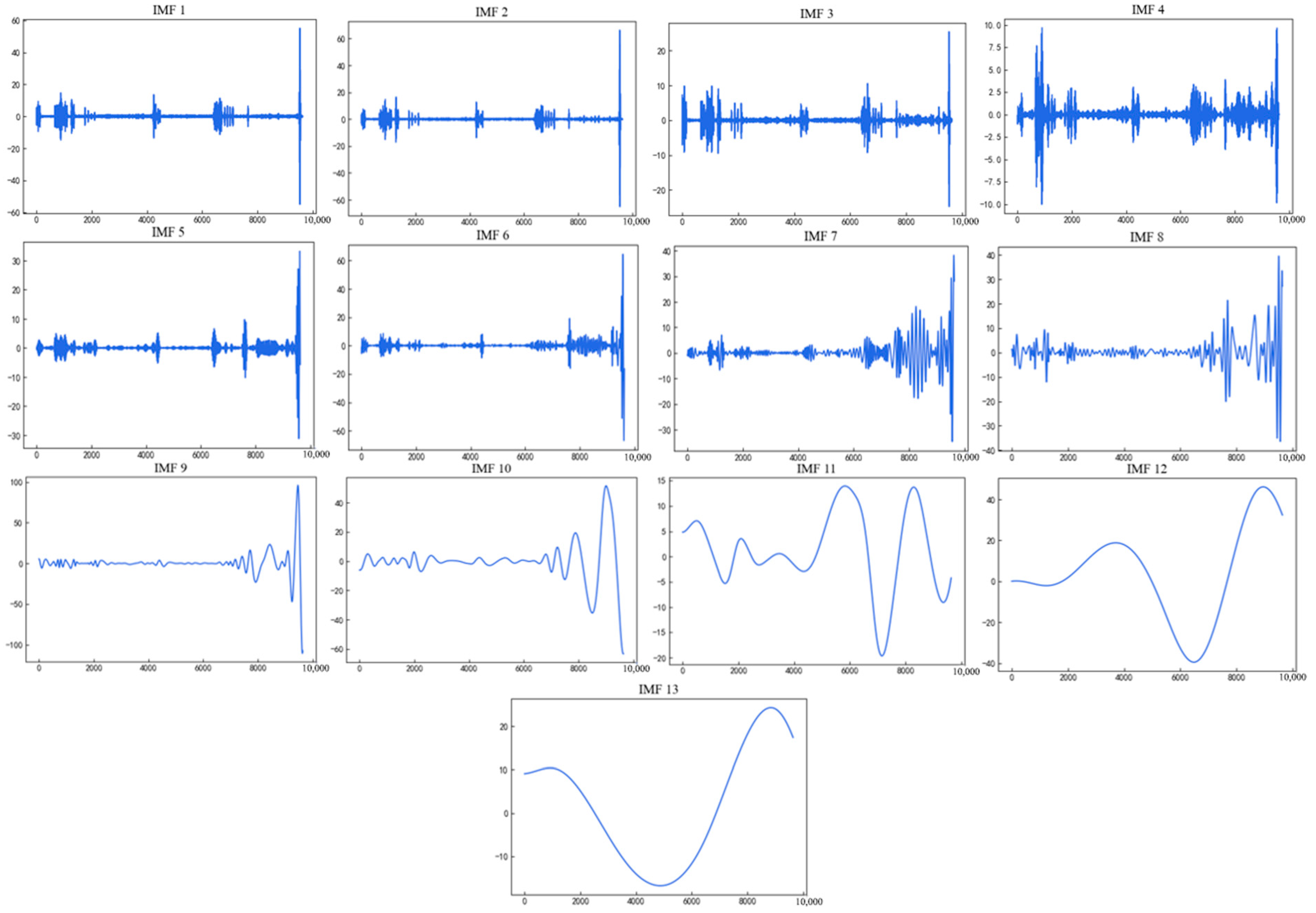
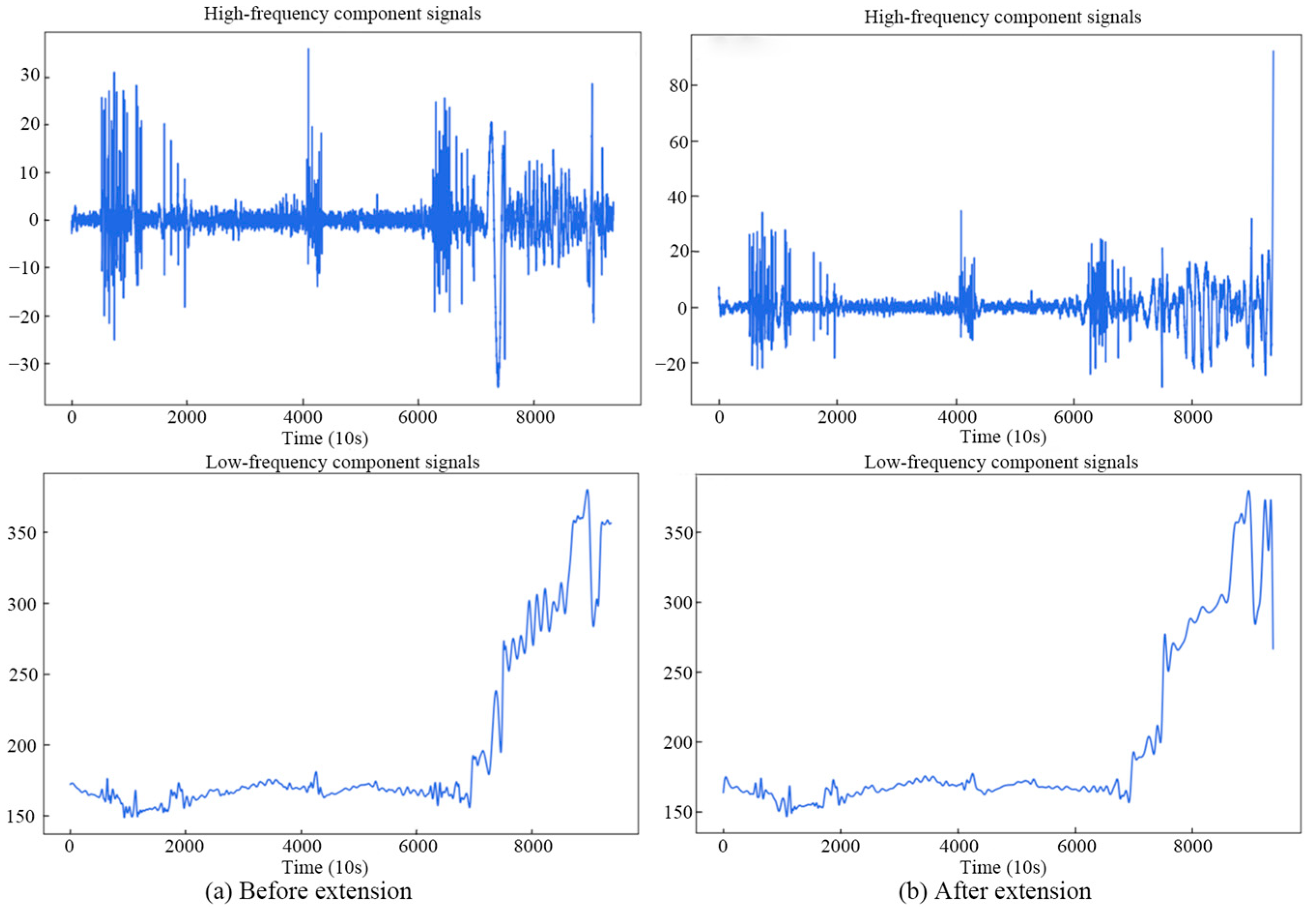
The component results of the upper guide X direction swing signal are shown in Figure 7 after EMD decomposition; Figure 8 shows the EMD decomposition results of the extended upper guide X direction swing signal based on the waveform matching extension method based on parameter ergodic optimization. The number of extreme values can reflect the fluctuation degree of each component, and the extreme point division method is used to reconstruct each decomposition component. The number of extreme points of each IMF component is shown in Table 2. In this paper, the appropriate extreme point value E = 200 is selected as the threshold to distinguish the components of high-frequency and low-frequency signals. Based on the decomposition results of the upper guide X direction swing signal of the unit, the high-frequency components of the unextended signal components are reconstructed from IMF1–IMF6, and the low-frequency component is reconstructed from IMF7–IMF12. The high-frequency component of the extended component is reconstructed by the IMF1–IMF7 combination and the low-frequency component is reconstructed by the IMF8–IMF13 combination. The results of the component reconstruction are shown in Figure 9.

4.3. Analysis of Experimental Results

The reconstructed high-frequency and low-frequency components are substituted into each prediction model. In the prediction process, the first 10 sets of historical data are taken as inputs to predict the next 1 set of swing signal values, and the upper guide X direction swing signal is divided into a training set and a test set according to the ratio of 8:2. The LSTMNN used in this study consists of 6 layers with 128 hidden nodes per layer and incorporates dropout technique at a rate of 0.1 to reduce model overfitting. In addition, a batch of 128 iterations with 150 epochs was chosen to train the input data. An Adam optimization algorithm was used to train the model efficiently for higher prediction accuracy. Figure 10 shows the prediction results of the high- and low-frequency components of the EMD + LSTMNN model and the W-EMD + LSTMNN fusion model.
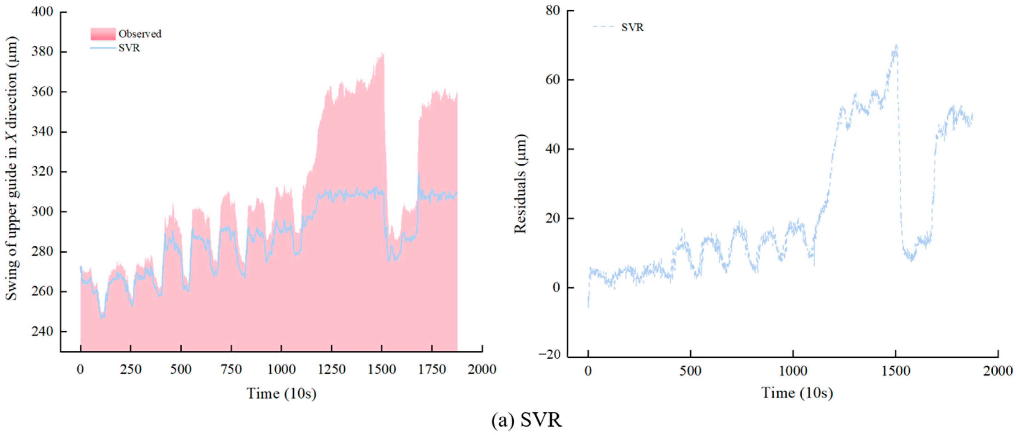
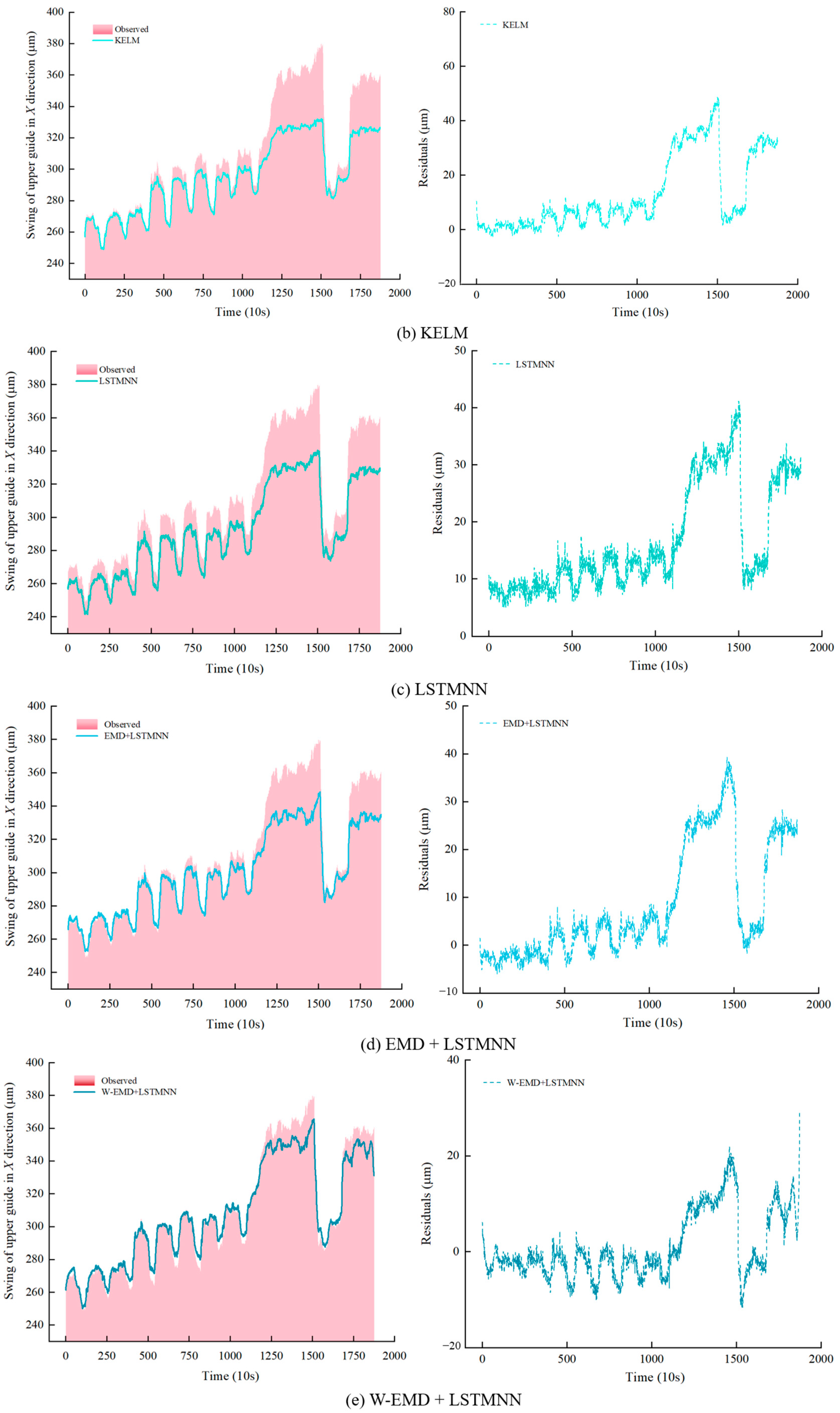
After the prediction results of the high- and low-frequency components of the upper guide X direction swing are obtained by the above model prediction, the final prediction results of the upper guide X direction swing of the hydropower unit are obtained by superimposing the equal weights of the component prediction results. In order to verify the superiority of the W-EMD + LSTMNN model in the signal decomposition algorithm as well as the effect of the swing signal prediction, SVR, KELM, a single LSTMNN model, and the traditional EMD + LSTMNN model are selected as the comparison models. Figure 11 shows the comparison results of trend prediction models on the upper guide X direction swing test set, where the histogram is the observed value of the upper guide X direction swing signal, and the solid line is the predicted value for each model. The comparison results of the observed and predicted values of the upper guide X direction swing signal and the prediction errors of each model are visualized in Figure 11. By analyzing the comparison chart of the prediction results of each model, it can clearly be seen that the error curve of the proposed model (W-EMD + LSTMNN) is closer to zero, and its fluctuation is smaller.
In this paper, four evaluation indexes, MAE, MAPE, MSE, and MSPE, are used to assess the prediction results of different models, based on the test set of the upper guide X direction swing data of the unit. The evaluation index results are shown in Table 3. The prediction errors of the three prediction models on the test set of the upper guide X direction swing signal are shown in Figure 12.
As can be seen from Table 3 and Figure 12, the evaluation index results of the W-EMD + LSTMNN fusion model proposed in this paper are better than those of other prediction models. Compared with SVR, the evaluation indicators MAE, MSE, MAPE, and MSPE obtained by KELM are generally lower; specifically, the reducing ratio in terms of MAE, MAPE, MSE, and MSPE is 39.36%, 40.25%, 35,14%, and 36.84%, respectively. For a single traditional LSTMNN model, on the unit upper guide X direction swing signal test set, the MAE is 11.3369 μ m , MAPE is 3.45%, MSE is 0.3285 μ m , and MSPE is 0.09%. Compared with the traditional LSTMNN model, the prediction effect of the prediction model combining the EMD signal decomposition algorithm with LSTMNN is improved. Where MAE is 9.4108 μ m , MAPE is 2.85%, and MSE is 0.2713 μ m , MSPE is 0.07%. Compared with the single LSTMNN model and the traditional EMD + LSTMNN combination model, the proposed W-EMD + LSTMNN fusion model in this paper has higher prediction accuracy, and its MAE, MAPE, MSE, and MSPE on the upper guide X direction swing signal test set are further reduced to 5.1112 μ m , 1.6%, 0.1489 μ m , and 0.04%, respectively. This avoids the problem of prediction error due to the endpoint effect of the traditional combination model and effectively improves the prediction accuracy.

5. Conclusions, Recommendations, Policy Insights, and Future Works

In this study, we propose a fusion model based on the waveform extension method to improve the empirical mode decomposition and the combination of long short-term memory neural networks for predicting the swing trend of hydropower units. The results show the following:
(1)
The waveform matching extended method based on parameter traversal optimization is used to process the x(t) of the simulated signal, and by comparing the similarity coefficient of EMD before and after extension, the method effectively suppresses the endpoint effect of EMD in the short-term data. Compared with the traditional method of predicting each component separately after EMD, the method of component reconstruction reduces the noise and interference in the prediction process, and effectively improves the stability and accuracy of the prediction model.
(2)
In order to verify the effectiveness of the proposed fusion model W-EMD + LSTMNN in improving the prediction accuracy, we studied the actual case of a sudden upward movement of the upper conductance slip rotor of unit 16F of a hydropower station in China, which led to the increase of the upper guide X direction swing. The fusion model effectively avoids the endpoint effect problem caused by the traditional empirical mode decomposition process, and compared with SVR, KELM, the single LSTMNN model, and the traditional EMD + LSTMNN combination model, it was found that W-EMD + LSTMNN, with the advantages of high prediction accuracy and strong generalization ability, successfully analyzed and predicted the increasing trend of an X direction pendulum of the upper guide, and discovered the potential hidden danger of the unit. The results show that the proposed W-EMD + LSTMNN fusion model has important application prospects in hydropower system operation state monitoring, and provides a reliable reference for hydropower unit trend prediction.
Since methods for suppressing the EMD endpoint effect are constantly evolving, whether the method proposed in this paper can serve as the best method for suppressing the endpoint effect requires extensive experimental studies. Therefore, in our future work, we will first investigate new methods to suppress the EMD endpoint effect and combine them with different machine-learning models to improve the quality of data decomposition as well as the prediction accuracy of the models for real-time prediction in practical applications. Secondly, the structure of the neural network model proposed in this paper is continuously optimized, and methods such as incorporating the attention mechanism are used to further improve the prediction accuracy and generalization ability of the prediction model. Finally, the results in Conclusion (2) were investigated in detail, and the scope of the dataset was enlarged or applied to different datasets in order to examine the practicability and effectiveness of the model proposed in this study.

Author Contributions

Conceptualization, D.L. and Z.T.; Methodology, D.L., Y.P. and H.H.; Supervision, D.L. and Z.T.; Validation, D.L., Y.P. and X.W.; Writing—original draft, D.L. and H.H.; Writing—review and editing, H.H. and X.W. All authors have read and agreed to the published version of the manuscript.

Funding

This research was funded by China Yangtze Power Co., Ltd. and Hubei Technology Innovation Center for Smart Hydropower (Grant No. Z152302039); Open Fund for Key Laboratory of Fluid and Power Machinery, Ministry of Education (Grant No. LTDL-2023012); National Key Research and Development Program of China (Grant No. 2022YFC3202805).

Data Availability Statement

The raw data supporting the conclusions of this article will be made available by the authors on request.

Conflicts of Interest

The authors declare that this study received funding from China Yangtze Power Co., Ltd. and Hubei Technology Innovation Center for Smart Hydropower. The funder was not involved in the study design, collection, analysis, interpretation of data, the writing of this article or the decision to submit it for publication. The remaining authors declare that the research was conducted in the absence of any commercial or financial relationships that could be construed as a potential conflict of interest.

References

  1. Poudyal, R. Renewable Energy and Other Strategies for Mitigating the Energy Crisis in Nepal. 2021. Available online: https://www.semanticscholar.org/paper/Renewable-Energy-and-Other-Strategies-for-the-in-Poudyal/fcded2d9d9cdadba02cb4dec0414787bde41818c#related-papers (accessed on 12 November 2024).
  2. Quaranta, E.; Bonjean, M.; Cuvato, D.; Nicolet, C.; Dreyer, M.; Gaspoz, A.; Rey-Mermet, S.; Boulicaut, B.; Pratalata, L.; Pinelli, M. Hydropower case study collection: Innovative low head and ecologically improved turbines, hydropower in existing infrastructures, hydropeaking reduction, digitalization and governing systems. Sustainability 2020, 12, 8873. [Google Scholar] [CrossRef]
  3. Li, X.; Chen, Z.; Fan, X.; Cheng, Z. Hydropower development situation and prospects in China. Renew. Sustain. Energy Rev. 2018, 82, 232–239. [Google Scholar] [CrossRef]
  4. Wang, Y.; Zou, Y.; Hu, W.; Chen, J.; Xiao, Z. Intelligent fault diagnosis of hydroelectric units based on radar maps and improved GoogleNet by depthwise separate convolution. Meas. Sci. Technol. 2023, 35, 025103. [Google Scholar] [CrossRef]
  5. Kumar, K.; Saini, R. A review on operation and maintenance of hydropower plants. Sustain. Energy Technol. Assess. 2022, 49, 101704. [Google Scholar] [CrossRef]
  6. Zhang, J.; Ma, Z.; Wang, X.; Wu, Q.; Zhang, L. Transient vibration of shafting in coupled hydraulic-mechanical-electrical-structural system for hydropower station during start-up process. Appl. Math. Model. 2023, 124, 860–880. [Google Scholar] [CrossRef]
  7. Singh, V.K.; Singal, S.K. Operation of hydro power plants—A review. Renew. Sustain. Energy Rev. 2017, 69, 610–619. [Google Scholar] [CrossRef]
  8. Xiao, L.; Wang, J.; Wang, B.; Jiang, H. China’s hydropower resources and development. Sustainability 2023, 15, 3940. [Google Scholar] [CrossRef]
  9. Tong, K.; Zhang, G.; Huang, H.; Qin, A.; Mao, H. A novel combined model for vibration trend prediction of a hydropower generator unit. Insight Non-Destr. Test. Cond. Monit. 2023, 65, 43–51. [Google Scholar] [CrossRef]
  10. Dao, F.; Zeng, Y.; Zou, Y.; Li, X.; Qian, J. Acoustic vibration approach for detecting faults in hydroelectric units: A review. Energies 2021, 14, 7840. [Google Scholar] [CrossRef]
  11. Huang, N.E.; Shen, Z.; Long, S.R.; Wu, M.C.; Shih, H.H.; Zheng, Q.; Yen, N.C.; Tung, C.C.; Liu, H.H. The empirical mode decomposition and the Hilbert spectrum for nonlinear and non-stationary time series analysis. Proc. R. Soc. Lond. Ser. A Math Phys. Eng. Sci. 1998, 454, 903–995. [Google Scholar] [CrossRef]
  12. Zare, M.; Nouri, N.M. End-effects mitigation in empirical mode decomposition using a new correlation-based expansion model. Mech. Syst. Signal Process. 2023, 194, 110205. [Google Scholar] [CrossRef]
  13. Chai, K.; Feng, S.W. Processing method of EMD endpoint effect based on SVRM extension. Vibroengineering Procedia 2020, 35, 70–75. [Google Scholar] [CrossRef]
  14. Xu, W.; Chen, S.H.; Wang, M.; Yang, W.; Wang, L. Eliminating the end effect of empirical mode decomposition using a cubic spline based method. Digit. Signal Process. 2021, 110, 102936. [Google Scholar] [CrossRef]
  15. Lv, C.; Zhao, J.; Wu, C.; Guo, T.; Chen, H. Optimization of the end effect of Hilbert-Huang transform (HHT). Chin. J. Mech. Eng. 2017, 30, 732–745. [Google Scholar] [CrossRef]
  16. Liang, L. Estimation of EMD Envelope Based on MQ Interpolation. Acad. J. Sci. Technol. 2022, 1, 36–39. [Google Scholar] [CrossRef]
  17. Song, S.D.; Yao, Z.C.; Wang, X.N. The summary of Hilbert-Huang transform. In Proceedings of the International Symposium on Photoelectronic Detection and Imaging 2013: Infrared Imaging and Applications, Beijing, China, 25–27 June 2013; SPIE: Dalian, China, 2013; pp. 748–754. [Google Scholar]
  18. Meng, S.; Kang, J.; Chi, K.; Die, X. Fault diagnosis of rolling bearing based on improved EMD algorithm. IOP Conf. Ser. Mater. Sci. Eng. 2020, 892, 12069. [Google Scholar] [CrossRef]
  19. Staudemeyer, R.C.; Morris, E.R. Understanding LSTM—A tutorial into long short-term memory recurrent neural networks. arXiv 2019, arXiv:1909.09586. [Google Scholar]
  20. Yu, Y.; Si, X.; Hu, C.; Zhang, J. A review of recurrent neural networks: LSTM cells and network architectures. Neural Comput. 2019, 31, 1235–1270. [Google Scholar] [CrossRef]
  21. Sherstinsky, A. Fundamentals of recurrent neural network (RNN) and long short-term memory (LSTM) network. Phys. D Nonlinear Phenom. 2020, 404, 132306. [Google Scholar] [CrossRef]
  22. Zhao, Z.; Chen, W.; Wu, X.; Chen, P.C.; Liu, J. LSTM network: A deep learning approach for short-term traffic forecast. IET Intell. Transp. Syst. 2017, 11, 68–75. [Google Scholar] [CrossRef]
  23. Zhou, K.B.; Zhang, J.Y.; Shan, Y.; Ge, M.F.; Ge, Z.Y.; Cao, G.N. A hybrid multi-objective optimization model for vibration tendency prediction of hydropower generators. Sensors 2019, 19, 2055. [Google Scholar] [CrossRef] [PubMed]
  24. Shan, Y.; Zhou, J.; Jiang, W.; Liu, J.; Xu, Y.; Zhao, Y. Vibration Tendency Prediction of Hydroelectric Generator Unit Based on Fast Ensemble Empirical Mode Decomposition and Kernel Extreme Learning Machine with Parameters Optimization. In Proceedings of 2018 11th International Symposium on Computational Intelligence and Design (ISCID), Hangzhou, China, 8–9 December 2018; pp. 287–290. [Google Scholar]
  25. Hu, N.; Kong, L.; Zheng, H.; Zhou, X.; Wang, J.; Tao, J.; Li, W.; Lin, J. Trend Prediction of Vibration Signals for Pumped-Storage Units Based on BA VMD and LSTM. Energies 2024, 17, 5331. [Google Scholar] [CrossRef]
  26. Qin, Q.; Lai, X.; Zou, J. Direct multistep wind speed forecasting using LSTM neural network combining EEMD and fuzzy entropy. Appl. Sci. 2019, 9, 126. [Google Scholar] [CrossRef]
  27. Wang, Y.; Xiao, Z.; Liu, D.; Chen, J.; Liu, D.; Hu, X. Degradation Trend Prediction of Hydropower Units Based on a Comprehensive Deterioration Index and LSTM. Energies 2022, 15, 6273. [Google Scholar] [CrossRef]
  28. Zhao, Q.; Lou, L.; Ouyang, B. Short-Time Traffic Flow Prediction Based on a Combined Model of EMD and LSTM. In Proceedings of the 2023 4th International Seminar on Artificial Intelligence, Networking and Information Technology (AINIT), Nanjing, China, 16–18 June 2023; pp. 424–429. [Google Scholar]
  29. Rong, Q. Research on EMD Method for Improving End Effect and Suppressing Modal Mixing. Ph.D. Thesis, Tianjin University, Tianjin, China, 2018. [Google Scholar]
  30. Zhang, C.; Zhou, J.; Li, C.; Fu, W.; Peng, T. A compound structure of ELM based on feature selection and parameter optimization using hybrid backtracking search algorithm for wind speed forecasting. Energy Convers. Manag. 2017, 143, 360–376. [Google Scholar] [CrossRef]
  31. Hyndman, R.J.; Koehler, A.B. Another look at measures of forecast accuracy. Int. J. Forecast. 2006, 22, 679–688. [Google Scholar] [CrossRef]
  32. Cohen, I.; Huang, Y.; Chen, J.; Benesty, J.; Benesty, J.; Chen, J.; Huang, Y.; Cohen, I. Pearson correlation coefficient. In Noise Reduction in Speech Processing; Springer: Berlin/Heidelberg, Germany, 2009; Volume 2, pp. 1–4. [Google Scholar]
  33. Danielsson, P.E. Euclidean distance mapping. Comput. Graph. Image Process. 1980, 14, 227–248. [Google Scholar] [CrossRef]
  34. Wang, L.; Zhang, Y.; Feng, J. On the Euclidean distance of images. IEEE Trans. Pattern Anal. Mach. Intell. 2005, 27, 1334–1339. [Google Scholar] [CrossRef]
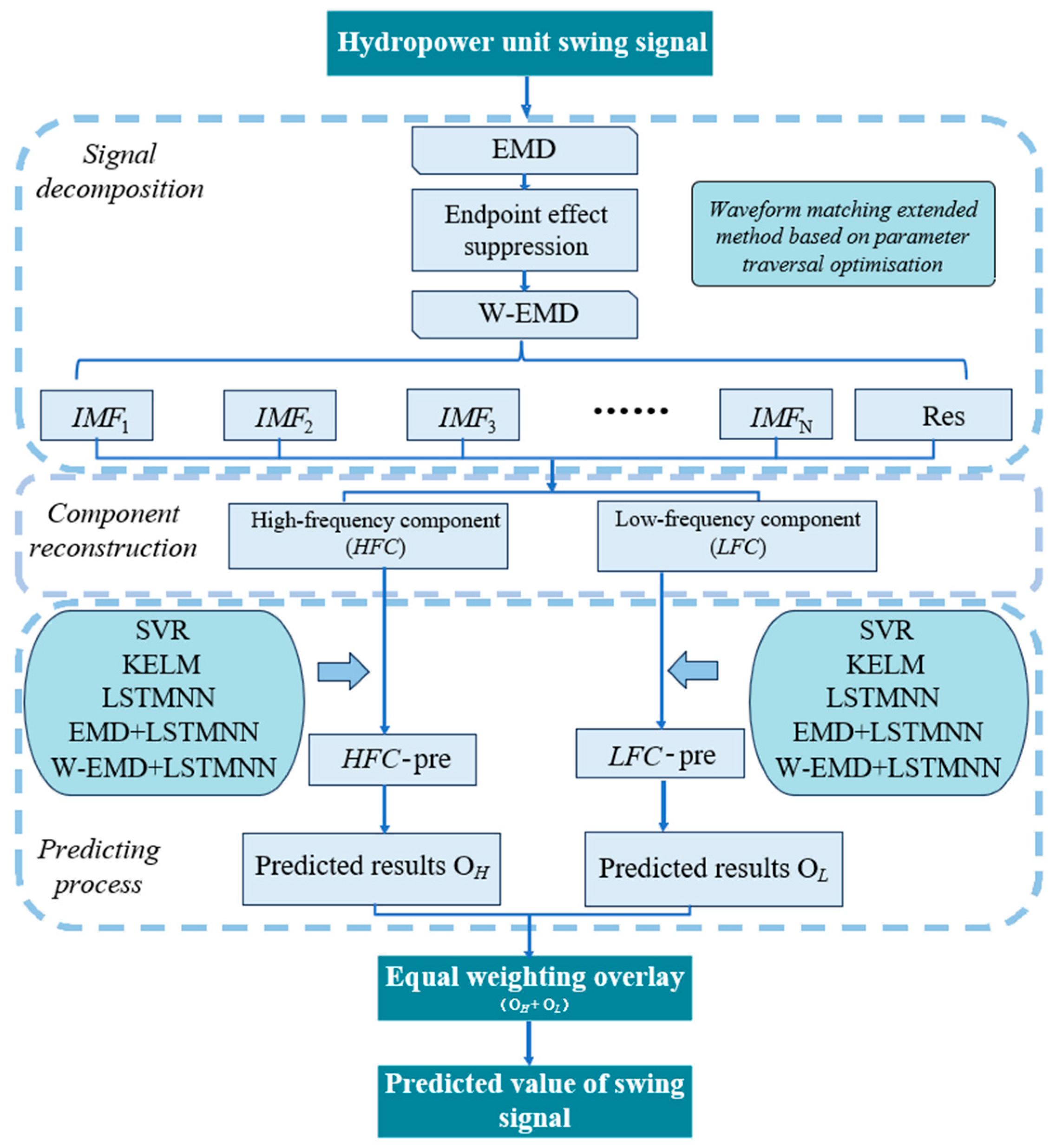
Figure 1. Flow diagram of the predictive model construction.
Energies 17 05847 g001
Figure 2. Simulation signal schematic.
Energies 17 05847 g002
Figure 3. Waveform matching extension.
Energies 17 05847 g003
Figure 4. Signal waveform diagram.
Energies 17 05847 g004
Figure 5. Comparison of EMD results before and after extension.
Energies 17 05847 g005
Figure 6. Upper guide X direction swing sequence of unit 16F. (a) Swing of upper guide in X direction data. (b) Swing data of the upper guide in the X direction after sliding average.
Energies 17 05847 g006
Figure 7. EMD results of the original data of the upper guide X direction swing.
Energies 17 05847 g007
Figure 8. EMD decomposition results after extension of the upper guide X direction swing.
Energies 17 05847 g008
Figure 9. IMF Component Reconstruction Results.
Energies 17 05847 g009
Figure 10. Prediction results for high- and low-frequency components. (a) The component predicted result of the empirical mode decomposition + long short-term memory neural network model (EMD + LSTMNN), (b) the predicted result of the waveform extension method empirical mode decomposition + long short-term memory neural network model (W-EMD + LSTMNN).
Energies 17 05847 g010
Figure 11. Comparison of prediction results of different models.
Energies 17 05847 g011aEnergies 17 05847 g011b
Figure 12. Prediction error of different models on the test set of MAE, MSE, MAPE, and MSPE.
Energies 17 05847 g012
Table 1. Comparison of similarity coefficients before and after extension.
Before ExtensionAfter Extension
IMF1 similarity coefficients0.99211.0012
IMF2 similarity coefficients0.96851.0009
IMF3 similarity coefficients0.89441.0008
Table 2. The number of extreme points of each IMF component after EMD.
Upper guide swing signalComponentIMF1IMF2IMF3IMF4IMF5IMF6
Number of extreme points6341406323471334803384
ComponentIMF7IMF8IMF9IMF10IMF11IMF12
Number of extreme points19494391552
After extension upper guide swing signalComponentIMF1IMF2IMF3IMF4IMF5IMF6
Number of extreme points6498419724571407840522
ComponentIMF7IMF8IMF9IMF10IMF11IMF12
Number of extreme points2631456735105
ComponentMF13-----
Number of extreme points2-----
Table 3. Evaluation indicators of each prediction model.
MAE   ( μ m ) MAPE (%) MSE   ( μ m ) MSPE (%)
SVR21.70250.06460.67080.0019
KELM13.15960.03860.43510.0012
LSTMNN11.34690.03450.32850.0009
EMD + LSTMNN9.41080.02850.27130.0007
W-EMD + LSTMNN5.11120.01600.14890.0004
Disclaimer/Publisher’s Note: The statements, opinions and data contained in all publications are solely those of the individual author(s) and contributor(s) and not of MDPI and/or the editor(s). MDPI and/or the editor(s) disclaim responsibility for any injury to people or property resulting from any ideas, methods, instructions or products referred to in the content.