Comparative Study of OLGA and LedaFlow Models for Mechanistic Predictions of Hydrate Transport Dynamics

Abstract

Gas hydrate formation in pipelines transporting multiphase fluids from petroleum reservoirs can lead to the formation of blockages, representing a significant flow assurance challenge. Key issues caused by hydrates include substantial increases in the viscosity of mixed liquid phases and the deposition of hydrates on the pipeline wall. This study compares two existing transient multiphase flow simulators, OLGA and LedaFlow, in terms of their estimation of hydrate formation effects on multiphase flow. Here, we compared in detail the hydrate kinetic models, parameters used, and initial condition setup approaches that influence hydrate formation and affect multiphase flow properties. Based on the comparison between the simulation results, it was found that using both simulators with default setups may not lead to comparable results under certain conditions. Adjusting input parameters, such as the stoichiometric coefficient and hydrate formation enthalpy, is necessary in order to obtain equivalent results. Hydrate modules in both simulators have also been applied to a field case. With appropriate setup, OLGA and LedaFlow produce comparable results during steady-state simulations, which align with field observations. This work provides guidelines for setting up OLGA and LedaFlow simulation models to obtain equivalent results.

1. Introduction

Oil and gas production in offshore settings is becoming increasingly complex as operators venture into deeper waters due to the depletion of shallow offshore petroleum resources [1]. This shift necessitates significant advancements in the conceptual design and operational strategies for these developments. The industry faces a range of challenging scenarios, especially involving multiphase flow dynamics along with other critical fluid-related phenomena. Key focus areas include optimizing pipe design and managing flow assurance issues.

Hydrate, wax, asphaltene, and scale are the four main production-chemistry-related issues in flow assurance [2]. The accumulation of these solids poses significant operational and economic risks in the oil and gas industry, potentially leading to reduced production rates, equipment failures, and production shutdowns. Among these issues, hydrate formation is particularly problematic due to its rapid occurrence and the difficulty in removal once formed, attributed to the dense and tough nature of hydrate blockages.

Gas hydrate forms under specific thermodynamic conditions that include high pressure, low temperature, and the presence of water and light hydrocarbons [3]. Several mechanisms that contribute to hydrate plugging have been proposed and illustrated in a conceptual picture, as shown in Figure 1. This illustration outlines four stages of hydrate formation and plugging [4]. Initially, water is dispersed within the continuous oil phase, increasing the surface area available for hydrate growth. This facilitates the formation of a hydrate shell around water droplets in the second stage. During the third stage, for hydrate particles surrounded with quasi-liquid layers, a capillary bridge forms and creates a cohesive force when hydrate particles collide with each other during the flow [5]. As hydrate particles start to agglomerate, they can cause viscosification in the slurry, which refers to an increase in viscosity due to the formation of hydrate particles and agglomerates. This process increases the resistance to fluid flow within the pipeline. Over time, this resistance can exceed the energy required to maintain transport, ultimately resulting in a blockage in the pipeline, known as a hydrate plug.

Another predictive model proposed for hydrate formation kinetics is the hydrate sponge model [7,8]. This model assumes hydrate particles to be porous structures under flow shear considering gas–liquid slug flow where the liquid phase is a water-in-oil emulsion. The authors present that due to crystal rotation and relative motion, hydrate crystallization primarily occurs within the walls of capillaries in the porous structure. The study also highlights the role of heat and mass transfer in hydrate formation, with heat transfer limitation causing the hydrate structure to remain porous for longer, and the competition between heat and mass transfer limitations determines the hydrate formation dynamics, influencing the rate and extent of mass conversion to hydrates.

Traditionally, gas hydrate management focused on preventing hydrate formation using a thermodynamics-based operating strategy [9]. This approach utilized a thermodynamic modeling tool, specifically based on minimizing Gibbs free energy, to perform hydrate phase equilibria predictions with flash calculations to estimate the appropriate dosage of thermodynamic hydrate inhibitor (THI, such as methanol or monoethylene glycol) [10]. Over the last two decades, the industry has shifted towards a risk-based approach to hydrate management, where hydrates are allowed to form, but the risk of any blockage is managed. The shift is driven by a deeper understanding of hydrate nucleation and formation, along with the kinetics of agglomeration and deposition. Kinetics modeling has become crucial for assessing hydrate risks in multiphase pipelines [6,11,12].

The hydrate model, CSMHyK (the Colorado School of Mines Hydrate Kinetics model), has been continuously developed over the last three decades and has emerged as the most widely used hydrate model among flow assurance engineers, particularly for assessing hydrate risks during transient events [6,13,14,15]. Its widespread acceptance as an industry reference tool is largely due to its integration (of the original CSMHyK model) with the OLGA software (version 2021.1.0), a transient multiphase flow simulator originally developed by the Institute of Energy Technology (IFE, Kjeller, Norway) in collaboration with SINTEF (The Norwegian Foundation for Industrial and Technical Research, Trondheim, Norway), which is currently commercialized by SLB (Schlumberger Limited, Houston, TX, USA). This seamless integration allows engineers to efficiently assess hydrate risks and model the implementation of hydrate mitigation measures across various operational scenarios. In 2005, Kongsberg Digital (Lysaker, Norway) introduced LedaFlow, a new multiphase flow performance simulator [16]. LedaFlow includes a module specifically designed to simulate hydrate formation and plugging in multiphase flow, providing additional tools for handling complex hydrate plugging risks in pipelines. Recent studies have applied the newly developed models for wax deposition and hydrate transport in LedaFlow to simulate conditions in a non-insulated oil pipeline in an offshore environment [17].

Given that both OLGA and LedaFlow possess predictive capabilities for flow assurance issues, this paper compares hydrate formation modeling in these two transient multiphase flow simulators. It focuses on examining how each simulator approaches hydrate kinetics and plugging, along with their methods for coupling the impacts of hydrate formation on multiphase flow. By analyzing and comparing OLGA and LedaFlow across various operations, the study aims to enhance understanding of their applicability to different scenarios and provide a reference for selecting the appropriate software for specific conditions. While previous studies have compared and simulated multiphase flow regimes and wax deposition using these simulators, hydrate transportation has not been specifically addressed [18,19,20]. This study delves into the underlying potential reasons for observed discrepancies between the simulation results of the two software programs, providing insights into their application for hydrate prediction that could also inform future updates or the development of next-generation hydrate models in multiphase flow transient simulation software.

2. Multiphase Flow Simulators and Hydrate Effects

Both OLGA and LedaFlow are one-dimensional transport models designed for the simulation of macroscale transport systems [21]. These models account for individual fluids or phases, including gas, oil, water, hydrate, or other flow assurance chemicals, and define a mass field as the movement of a particular form of the fluid, either in continuous or dispersed form [22]. Originally based on the two-fluid model, these simulators solve the conservation equations for each individual mass field across the cross-section of the pipeline [16,23,24], representing each field by mass, momentum, and energy equations. The multiphase flow simulators use a three-fluid model that accounts for the presence of three separate fluid phases, including gas, oil, and water [16,24,25,26]. By solving this set of conservation equations, values for pressure, temperature, velocity, and phase volume fractions as a function of space and time can be obtained.

Multiphase flow can be categorized into distributed and separated flow regimes [27]. The distributed regime includes bubble and slug flow, while the separated regime includes stratified (smooth or wavy) and annular-mist flow. OLGA determines flow regimes based on a minimum-slip criterion, which selects the regime that yields the minimum gas velocity for a given pressure drop, whereas LedaFlow identifies flow regimes through local phase distribution by calculating the no-slip liquid holdup and the mixture Froude number using Beggs and Brill approach [16,24,28]. Identifying the flow regime is crucial, as the closure relationships used to solve the conservation equations, such as wetted perimeters and friction factors, depend on the flow regime. The liquid holdup and pressure drop will be determined hereafter based on the flow regime.

Hydrate models in these simulators impact multiphase flow calculations within pipeline systems. In the mass conservation equation, the mass transfer rate between the gas and liquid or water phases is modified by the hydrate kinetics model. Additionally, the entrainment and deposition rates can be updated if the formed hydrates move between different mass fields. Hydrate formation also affects the momentum of flow phases by altering phase distribution, density, and viscosity. The change increases flow resistance, potentially leading to hydrate plug formation, as indicated by the friction factor. Furthermore, in the energy balance equation, hydrate formation and dissociation reactions influence temperature distribution due to their exothermic and endothermic nature, respectively.

3. Methodology

The study conducts a comparative analysis of the modeling of multiphase flow and hydrate behavior using internal hydrate modules in two simulation software: OLGA version 2021.1.0 and LedaFlow version 2.8.264.024. The comparison is carried out across two scenarios: a simplified horizontal pipeline and an actual field setup. In both scenarios, simulations are run first with the hydrate module inactivated and then with the hydrate module activated to separate the effects of multiphase flow and the respective hydrate models.

The horizontal pipeline scenario is designed to closely examine specific models and properties of hydrate formation. In the simulation, a 50 km horizontal pipeline is used, with a flow boundary (closed node in OLGA) connected to a pressure boundary at 4 °C and 80 bar, which are typical subsea conditions. The pipe has a diameter of 30 cm and is made of carbon steel with a density of 7850 kg/m³, a heat capacity of 470 J/kg$·$K, and a thermal conductivity of 45 W/m$·$K. It has a wall thickness of 20 mm and no insulation. A mass source introduces fluid into the flowline. The standard flow rate of oil is 5432.5 Sm³/d, with a 20% water cut and a gas–oil ratio (GOR) of 180 Sm³/Sm³. Detailed fluid properties are listed in Wang et al. [29]. A summary of the simulation parameters is also presented in

Table 1. Specifications for the horizontal pipeline simulation setup.

Pipeline length	50 km
Pipeline inner diameter	30 cm
Water cut	20 vol.%
Gas–oil ratio	180 Sm3/Sm3

.

In contrast, the real field setup, incorporating fluid properties and pipeline geometry from an actual field case [30], is used to evaluate the prediction of hydrate plug formation in pipelines. The schematic of the simulation model is presented in Figure 2, and the bathymetry of the well and flowline is shown in Figure 3. The fluid has a water cut of 15 vol.% with a GOR of 2500 Sm³/Sm³. An Inflow Performance Relationship (IPR) model is used with a productivity/injectivity index of 29.5 Sm³/d/bar. The well pressure is 225 bara with a temperature of 131 °C, while the end manifold is set to a pressure of 120 bara and a temperature of 15 °C. In this comparative study, only steady-state continuous production is modeled. Hydrate model behaviors during transient operations, such as shut-in and restart periods, are out of the scope of this work.

Table 2. Specifications for the field simulation setup.

Flowline length	11.2 km
Flowline inner diameter	30.48 cm
Water cut	15 vol.%
Gas–oil ratio	2500 Sm3/Sm3

also provides a summary of the simulation parameters used in the study.

4. Hydrate Module Comparison Used in Simulators

4.1. Hydrate Models Used in OLGA and LedaFlow

Hydrate formation alters the mass transfer and flow resistance, impacting the mass and momentum balance in the multiphase flow equations. The hydrate reaction kinetics and hydrate slurry viscosity models are key components of the hydrate module that contribute to the mass and momentum balance calculations.

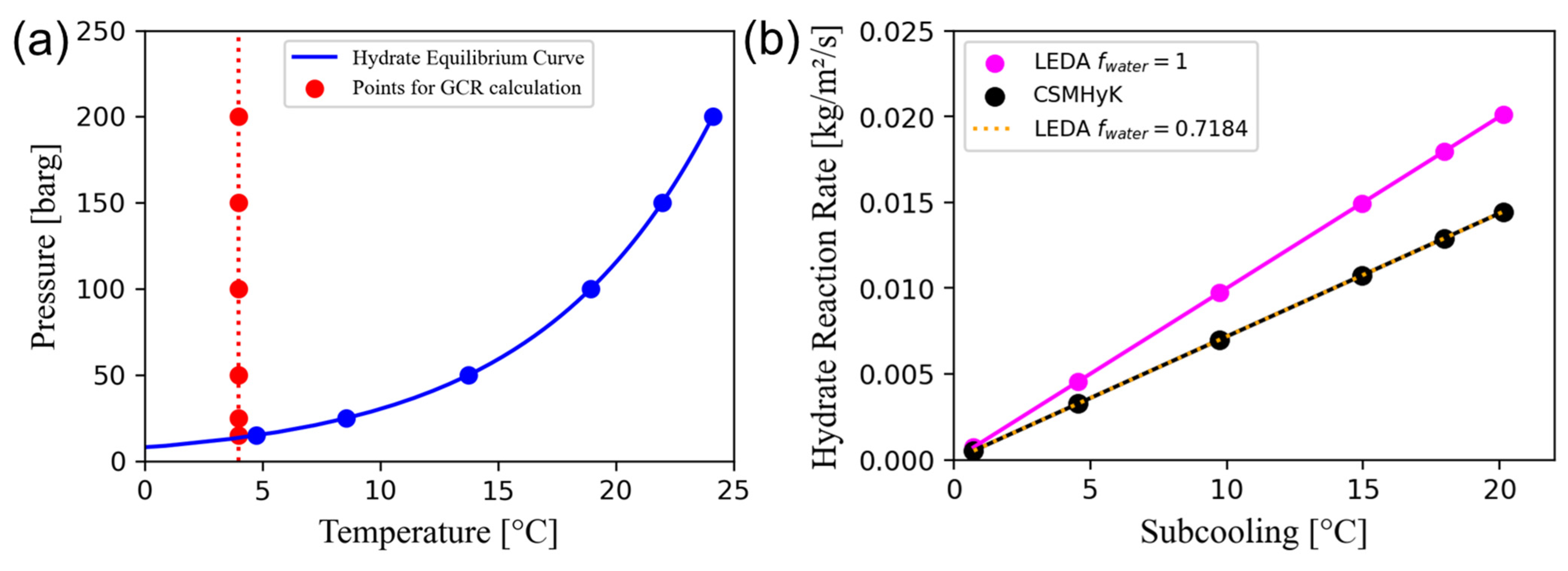
4.1.1. Hydrate Kinetics Model

A similar model of hydrate reaction rate calculation is used in both LedaFlow and OLGA. In LedaFlow, the reaction rate (${\mathsf{\Gamma }}_{net}^{hydrate}$ with unit of ${\displaystyle \frac{\mathrm{k}\mathrm{g}}{{\mathrm{m}}^3·\mathrm{s}}}$) depends on the specific surface area of hydrate particles ($A_{hydrate}$) and water droplets ($A_{water}$), and the subcooling $(T_{equilibrium}-T_{average})$, which is the difference between equilibrium temperature ($T_{equilibrium}$) and average temperature ($T_{average}$):

$${\mathsf{\Gamma }}_{net}^{hydrate}=c(f_{hydrate}{A}_{hydrate}+f_{water}{A}_{water})(T_{equilibrium}-T_{average})$$

(1)

A rate correction factor, $c$, is implemented to scale up or down the hydrate growth rate, which has a default value of ${10}^{-5}{\displaystyle \frac{\mathrm{k}\mathrm{g}}{{\mathrm{m}}^2·\mathrm{K}·\mathrm{s}}}$. Both $f_{hydrate}$ and $f_{water}$ are tuning factors for the surface area of hydrate formation, which can be adjusted in LedaFlow.

The equation also calculates the surface area of hydrate and water per unit volume, with unit of ${\displaystyle \frac{{\mathrm{m}}^2}{{\mathrm{m}}^3}}$, as:

$$A_{hydrate}={\displaystyle \frac{6V_{hydrate}}{d_{32}}}$$

(2)

$$A_{water}={\displaystyle \frac{6V_{water}}{d_{32}}}$$

(3)

In these equations, $V_{hydrate}$ and $V_{water}$ represent the volume of hydrate and water phases, respectively. The Sauter mean diameter $d_{32}$ used to calculate surface area, has a default value of 40 $\mathsf{\mu }\mathrm{m}$, which is a constant value instead of being calculated with empirical correlations.

In LedaFlow, the model assumes that hydrate only forms when the mixture velocity is above a user-defined value, which defaults to 0.1 m/s. This mimics the limited hydrate formation during shutdown as a thin layer of hydrate keeps the hydrate former and water from reacting.

In OLGA-CSMHyK, a similar intrinsic first-order kinetics thermodynamic-driving model is used to calculate the gas consumption rate, which is associated with the hydrate growth rate. The reaction rate is a function of a calculated rate correction factor, $u$, the kinetic constants and system temperature, $k_1\mathrm{e}\mathrm{x}\mathrm{p}({\displaystyle \frac{k_2}{T_{system}}})$ [${\displaystyle \frac{\mathrm{k}\mathrm{g}}{{\mathrm{m}}^2·\mathrm{K}·\mathrm{s}}}$], the specific surface area of water droplets, $A_{water}$ $[{\displaystyle \frac{{\mathrm{m}}^2}{{\mathrm{m}}^3}}]$, and subcooling ($T_{equilibrium}-T_{system}$) $\left[\mathrm{K}\right]$.

$${\mathsf{\Gamma }}_{net}^{hydrate}=u{k}_1\mathrm{e}\mathrm{x}\mathrm{p}({\displaystyle \frac{k_2}{T_{system}}})A_{water}(T_{eq}-T_{system})$$

(4)

The kinetic constants are $k_1=7.3548\times {10}^{17}$ [${\displaystyle \frac{\mathrm{k}\mathrm{g}}{{\mathrm{m}}^2·\mathrm{K}·\mathrm{s}}}$], $k_2=-\mathrm{13,600}$ $\left[\mathrm{K}\right]$, which were regressed from the gas consumption rate measurements performed by Vysniauskas and Bishnoi [31] and Englezos et al. [32] during the formation of mixed methane and ethane hydrate at different temperatures and subcooling. Given that the measurements for regression were conducted in a semi-batch stirred tank reactor, a scaling factor $u$ was introduced to account for mass and heat transfer resistances in the model [33]. The value of $u$ was set to 0.02 in order to match the flowloop data used to validate the model [6].

It should be noted that there are two major differences between OLGA and LedaFlow in the hydrate kinetics model: the correction factor and the specific surface area for hydrate formation. In LedaFlow, the correction factor is set as a constant value, whereas in OLGA-CSMHyK, it varies with the system temperature. For a specific surface area of 100 ${\displaystyle \frac{{\mathrm{m}}^2}{{\mathrm{m}}^3}}$ and a constant system temperature of 4 °C, the data points taken for the gas consumption rate comparison and the corresponding hydrate equilibrium curve are shown in Figure 4a. Figure 4b demonstrates that the $f_{water}$ term needs to be adjusted to achieve a comparable hydrate reaction rate to that given by CSMHyK ($f_{hydrate}$ is set to be 0 in LedaFlow). Therefore, unless the system temperature remains relatively constant during hydrate formation or has reached a steady state, this difference may still lead to discrepancies in the hydrate reaction rate even after tuning the factor $f_{water}$. Overall, it is important to note that a single correction factor cannot be applied to match all reaction rates at various subcooling levels. If the temperature changes from high to low, the kinetic rate in CSMHyK would depend on both the temperature and subcooling, whereas in LedaFlow, it only depends on subcooling.

LedaFlow provides an additional option to account for the surface area involved in hydrate formation by adjusting the $f_{hydrate}$ parameter. This adjustment considers the nucleation probability, reflecting the process of homogeneous secondary nucleation, where small hydrate nuclei break off from existing particles and serve as new sites for further growth. In water-in-oil emulsions, smaller water droplets lead to a higher specific surface area. However, similar to ice formation in such emulsions, smaller droplets reduce the probability of crystallization [34]. By setting the values of $f_{hydrate}$ and $f_{water}$, users can balance the effects of nucleation and surface area availability for hydrate formation based on the system. LedaFlow also includes a hydrate hold-time option to control the nucleation process, specifying the time required to form hydrates at different degrees of subcooling if experimental data are available.

In contrast, OLGA-CSMHyK assumes immediate nucleation once the nucleation subcooling defaulted to 6.5 °F, is met [35]. Hydrate formation occurs only at the water–oil interface around the water droplets, with the hydrate particle size matching the mean diameter of the water droplets. This diameter can be set as a fixed value or calculated using Boxall’s correlation based on Weber and Reynolds numbers [36].

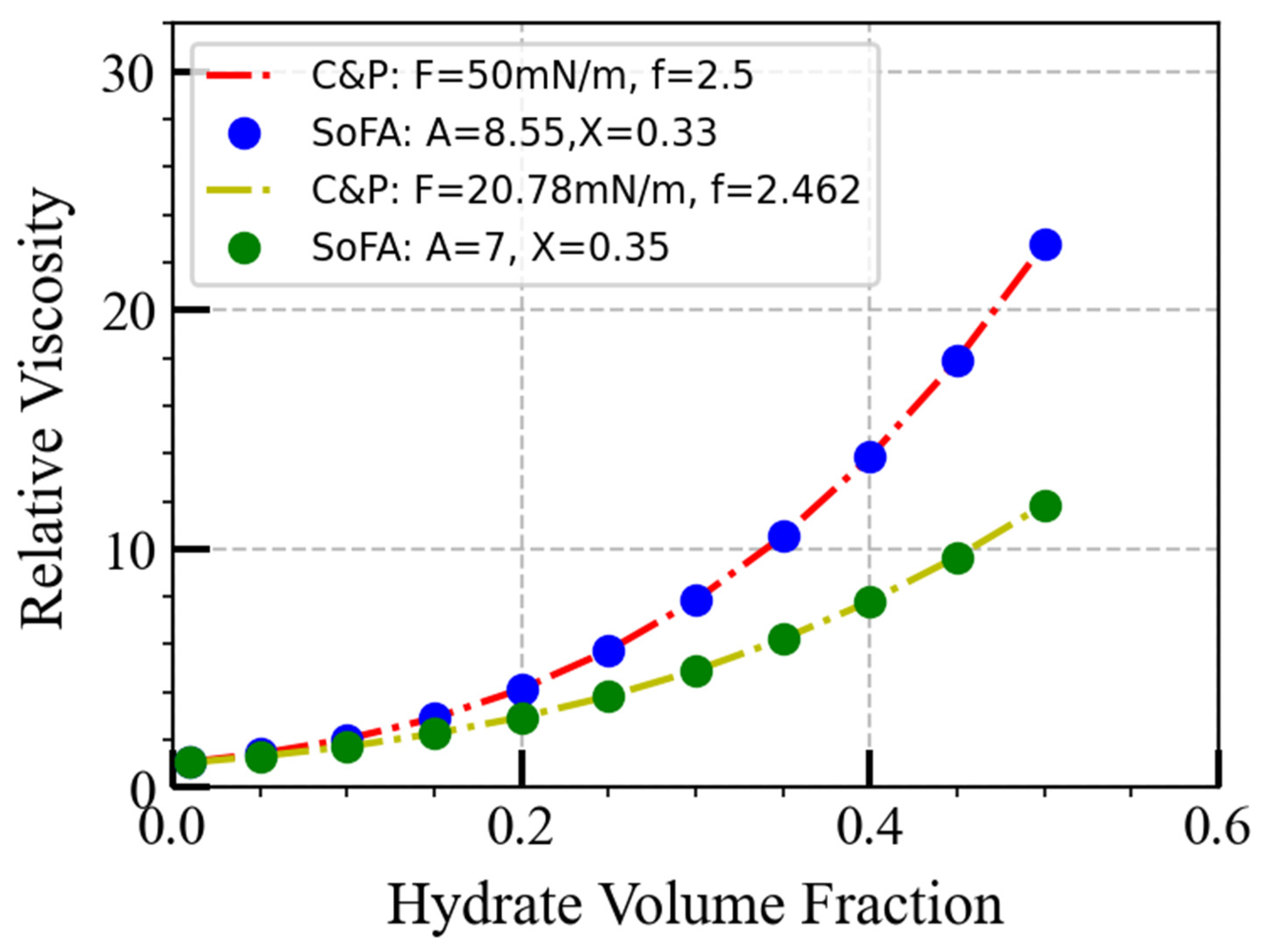
4.1.2. Hydrate Viscosity Model

Hydrate formation increases the viscosity of the slurry, leading to a high pressure drop in the flow. The agglomeration is considered and assumed well dispersed in the continuous phase. There are two different viscosity models available for hydrate transport that consider the impact of agglomeration.

For modeling solid/liquid suspensions that remain Newtonian, where the hydrate volume fraction is lower than 0.6 and interparticle interactions must be considered, the Thomas model is used as a semi-empirical expression for the relative viscosity, as shown in Equation (5).

$${\displaystyle \frac{\mu }{{\mu }_o}}=1+2.5V_{hydrate}+C{V}_{hydrate}^2+A(\exp \left(B{V}_{hydrate}\right)-1)$$

(5)

where the default values of slurry viscosity parameters A, B, and C are 0.00273, 16.6, and 10.05, respectively.

For non-Newtonian fluid, which is mostly the case, the Suspension of Fractal Aggregates (SoFA) model is used to simulate the relative viscosity of the hydrate slurry [37], as shown in Equation (6).

$${\displaystyle \frac{\mu }{{\mu }_o}}={\displaystyle \frac{1-A{V}_{hydrate}{\tau }^{-X}}{{\left(1-\frac{A{V}_{hydrate}{\tau }^{-X}}{V_{hydrate,max}}\right)}^2}},V_{hydrate,max}={\displaystyle \frac{4}{7}}$$

(6)

In OLGA-CSMHyK, hydrate agglomeration is explicitly modeled by conducting a steady-state balance on the cohesion and shear forces between particles. The Camargo and Palermo (C&P) model, shown in Equation (7), is used to calculate the maximum agglomerate size in the hydrate module. This model is based on the mechanism of aggregate breakup in shear flows, where the maximum size of aggregates is determined by the balance between shear stress and cohesive force between particles, as proposed by Mühle in the context of the erosion of microflocs [5,38]. In this model, $d_A$ is the hydrate agglomerate diameter, $d_p$ is the hydrate particle diameter, $\phi$ is the hydrate particle volume fraction, ${\phi }_{max}$ is the maximum packing fraction (assumed to be 4/7), $F_A$ is the cohesive force, $f$ is the fractal dimension (assumed to be 2.5), ${\mu }_o$ is the oil viscosity, and $\gamma$ is the shear rate [5]. This phenomenological model explains the non-Newtonian behavior of the hydrate suspension in the oil. It assumes that the hydrate particles forming agglomerates are spherical with identical droplet sizes in the same iteration.

$${({\displaystyle \frac{d_A}{d_P}})}^{4-f}-{\displaystyle \frac{{F_A\left[1-\frac{\phi }{{\phi }_{max}}{\left(\frac{d_A}{d_P}\right)}^{3-f}\right]}^2}{{d_P}^2{\mu }_o\gamma \left[1-\phi {\left(\frac{d_A}{d_P}\right)}^{3-f}\right]}}=0$$

(7)

To capture the increase in viscosity caused by hydrate formation and agglomeration, CSMHyK uses a modified Mills’s equation to calculate the relative viscosity (${\mu }_r$) of the hydrate slurry relative to the continuous oil phase, as shown in Equation (7) [39]. This calculation is based on the effective volume fraction (${\phi }_{eff}$) of the hydrate aggregates, described in Equation (9), which accounts for the fractal structure of the hydrate agglomerates. In this context, ${\phi }_{max}$, represents the maximum particle packing fraction of spheres with the same diameter.

$${\mu }_r={\displaystyle \frac{1-{\phi }_{eff}}{({1-\frac{{\phi }_{eff}}{{\phi }_{max}})}^2}}; {\phi }_{max}={\displaystyle \frac{4}{7}}$$

(8)

$${\phi }_{eff}=\phi {\left({\displaystyle \frac{d_A}{d_P}}\right)}^{3-f}$$

(9)

It should be noted that even though the SoFA and C&P models have different approaches to modeling the rupture of aggregates, both models share the same base as Equation (7). The SoFA model is based on the power law expression discussed by Potanin, which describes the behavior of aggregates in shear flow [40]. Instead of using Equation (9) to calculate effective hydrate volume fraction, the SoFA model uses Equation (10).

$${\phi }_{eff}={\phi }_{hyd}{A\tau }^{-X}$$

(10)

When shear stress used in the SoFA model is converted from the constant shear rate (500 s⁻¹) and viscosity calculated with the C&P model using Newton’s law of viscosity $\mu ={\displaystyle \frac{\tau }{\gamma }}$, Figure 5 shows that C&P and SoFA models are comparable as long as equivalent parameters are used. The explicit relationship between the parameters used in both models is listed in Equations (11) and (12), where

$$A={({\displaystyle \frac{\frac{F_A}{r_p}}{{2d}_p}})}^{{\displaystyle \frac{3-f}{4-f}}}$$

(11)

$$X={\displaystyle \frac{3-f}{4-f}}$$

(12)

The ${\displaystyle \frac{F_A}{r_p}}$ is the cohesive force given by Micromechanical force (MMF) measurements, corresponding to the cohesive force divided by the harmonic mean radius of the two hydrate particles. The default parameters used in OLGA-CSMHyK are a fractal dimension of 2.5, a droplet size of 40 $\mathsf{\mu }\mathrm{m}$, and a cohesive force of 50 mN/m, based on experimental measurements [14]. These values correspond to A of 8.55 and X of 0.333 used in LedaFlow. The default values of A and X in LedaFlow are 7 and 0.35, respectively, corresponding to a fractal dimension of 2.5, a droplet size of 40 $\mathsf{\mu }\mathrm{m},$ and a cohesive force of 27 mN/m. Therefore, with the default setups of both simulators, it is expected that LedaFlow will give slightly lower viscosity due to the lower cohesive force. It should also be noted that as the hydrate volume fraction approaches the maximum packing fraction, the relative viscosity approaches infinity.

4.2. Hydrate-Relevant Parameters Implemented in OLGA and LedaFlow

Both the stoichiometric coefficient and hydrate formation enthalpy are critical parameters in hydrate simulation. The stoichiometric coefficient affects the kinetics of hydrate formation and dissociation, representing the water-to-gas ratio in hydrates used to predict the formation and stability of gas hydrates accurately. In OLGA-CSMHyK, an embedded value of 6.85 is used as the stoichiometric coefficient, while in LedaFlow, the default value is 4.8, though it can be adjusted. The stoichiometric coefficient, known as the hydration number, has been studied since the discovery of hydrates.

The cell structures of hydrate crystals have been investigated, with the ideal unit cell formula for structure I (sI) hydrate being 6(5¹²6²)·2(5¹²)·46H₂O. For the structure II (sII) hydrate, commonly formed in production flowlines, the ideal unit cell formula is 8(5¹²6⁴)·16(5¹²)·136H₂O. The ideal molar-based hydration number is 5.75 for the sI hydrate and is 5.67 (if both large and small cages can be filled) or 17 (if only large cages can be filled) for the sII hydrate. However, the actual hydration number will be higher according to system conditions, guest composition, and the size of guest gas molecules, as it is impossible for all cavities to be occupied. Various methods can be used to verify the actual hydration number, including direct macroscopic methods, such as measuring the amount of gas released during hydrate dissociation and calorimetric, as well as microscopic measurements, such as single crystal or powder X-ray and neutron diffraction. Villard’s rule, which provides a general guideline that the hydration number for many gas hydrates is approximately 6, has proven to be a good rule of thumb in many cases [3]. Therefore, it is recommended that the default number be close to this value for approximation. For better accuracy, it would be more convenient if users could adjust the hydration number in the graphic user interface based on the field composition when running simulations.

The exothermal reaction of hydrate formation is captured by both LedaFlow and OLGA. During hydrate formation, heat release leads to a temperature increase, which reduces the hydrate formation rate. Therefore, if the hydrate formation enthalpy differs between simulators, different hydrate formation kinetics are expected. In LedaFlow, a constant reaction heat is used, set to 477.4 kJ/kg with respect to the mass of the hydrate. This value cannot be changed by users. However, in OLGA-CSMHyK, the hydrate formation enthalpy can be adjusted by users, with a default value of 4100 kJ/kg with respect to the mass of methane gas (i.e., the hydrate former component). The primary reason OLGA-CSMHyK allows for adjustable hydrate formation enthalpy is that the enthalpy value depends not only on the hydrogen bonds within the crystal but also on the occupation of the cavities. Users can adjust this value based on the field composition to account for these factors when necessary. It should also be noted that the differing magnitudes of enthalpy between LedaFlow and OLGA-CSMHyK are due to the basis of mass, whether it is based on the mass of the hydrate or the mass of the gas forming the hydrate.

The simplified horizontal pipeline simulation was performed to compare the setup differences between the models. After tuning the hydrate kinetics correction factor and surface area to be equivalent, it can be seen in Figure 6 that default setups result in a hydrate volume fraction difference of approximately 24%, with a maximum hydrate volume fraction of 9.7 vol.% given by LedaFlow and 7.6 vol.% given by OLGA. The hydrate formation enthalpy is adjusted in OLGA; a lower enthalpy value results in less hydrate formation since the heat released inhibits further hydrate formation. In LedaFlow, adjusting the hydration number shows that a higher value leads to a lower hydrate volume fraction, as more gas is needed to form a certain amount of hydrate. The simulation gives equivalent results when adjusting the stoichiometric coefficient (SC) to be 6.85 in LedaFlow and hydrate formation enthalpy ($H$) to be 3500 kJ/kg with respect to the mass of methane gas, which is equivalent to 468.7 kJ/kg with respect to methane hydrate in OLGA. Nevertheless, the parameters should be adjusted based on actual conditions when applying them to field simulation.

4.3. Coupling of Hydrate Models with the Multiphase Flow Simulator

When coupling the hydrate model with the multiphase flow simulator, the difference is mainly from the momentum and energy balance equations. The heat transfer models embedded in LedaFlow and OLGA have been compared to investigate the difference.

When updating the heat transfer model in multiphase flow, both OLGA and LedaFlow calculate the temperature of the fluid and the pipe wall, assuming radial heat conduction through concentric wall layers. They determine an internal heat transfer coefficient for the heat transfer from the fluid to the inner pipe wall. If an additional wall layer forms due to the deposition of the hydrate phase, it could increase resistance to the overall heat transfer ($OHTC$). $OHTC$ measures the total resistance to heat transfer through a series of thermal resistances, including convective resistance from the fluid inside the pipe ($R_{conv,i}$), conductive resistance from the pipe wall ($R_{cond}$), and convective resistance from the fluid outside the pipe ($R_{conv,o}$), as shown in Equation (13).

$$OHTC={\displaystyle \frac{1}{R_{conv,i}+R_{cond}+R_{conv,o}}}={\displaystyle \frac{1}{\frac{1}{h_{i}2\pi r_{i}L}+\frac{\mathrm{l}\mathrm{n}\left(\frac{r_o}{r_i}\right)}{2\pi kL}+\frac{1}{h_{o}2\pi r_{o}L}}}$$

(13)

Here, $k$ is the thermal conductivity of the pipe material, $h_i$ and $h_o$ are the inner and outer convective heat transfer coefficients, respectively, $r_i$ and $r_o$ are the inner and outer radii of the pipe, respectively, and L is the length of the pipe section. This section is focused on comparing the heat transfer model setups and performance in the absence of hydrate between OLGA and LedaFlow. The horizontal pipeline simulation is used for the comparison.

Different options to set up the heat transfer model in OLGA and LedaFlow are summarized in

Table 3. Basic approaches to set up heat transfer models in OLGA and LedaFlow.

Options	Settings		Descriptions
	OLGA	LedaFlow
1	Temperature = OFF	Temperature calculations = No	Constant temperature, the energy equation is disabled
2	Temperature = Ugiven Heat transfer coefficient = Uvalue	Wall heat transfer = Uvalue	User-defined overall heat transfer coefficient
3	Temperature = Fastwall Heat transfer coefficient = HOuterOption	Wall heat transfer = Walls (static)	The heat transfer coefficient is defined or calculated; heat storage is neglected in the wall
4	Temperature = Wall Heat transfer coefficient = HOuterOption	Wall heat transfer = Walls (dynamic)	The heat transfer coefficient is defined or calculated; heat storage in the wall is included

. The first option is fairly straightforward and comparable, as it involves no calculations beyond the user-defined parameters. This option is rarely used since the energy conservation equation is disabled, but it can serve as a simplified approach for specific purposes. Options 2, 3, and 4 include calculations of heat transfer coefficients, which lead to some discrepancies.

For Option 2, the U-value is defined differently in OLGA and LedaFlow. In OLGA, the U-value is defined to be consistent with the $OHTC$. In contrast, LedaFlow defines the U-value as a combined heat transfer coefficient for the pipe, considering only the pipe wall and the external heat transfer coefficient of the pipe. The internal heat transfer coefficient, which defines the convective resistance inside the pipe, is calculated separately. This setup typically results in a lower $OHTC$ compared to the U-value specified.

When comparing Options 3 and 4, it was found that the internal convective heat transfer coefficient is modeled differently between OLGA and LedaFlow. Correlations based on dimensionless numbers, including the Reynolds number (which characterizes the ratio of inertial forces to viscous forces in the flow), the Prandtl number (which represents the ratio of momentum diffusivity to thermal diffusivity), and the Nusselt number (which indicates the enhancement of heat transfer through a fluid layer compared to pure conduction) are used. Additionally, LedaFlow solves the energy conservation equations for each phase individually rather than for the mixture, as OLGA does [24]. As a result, the heat transfer coefficient is updated for each phase and the wall, as well as between the phases, in LedaFlow before being averaged out. This is another source of inconsistency between the results provided by LedaFlow and OLGA.

When using the same setups and input parameters in OLGA and LedaFlow, it was found that the higher the flow rate of the internal or surrounding fluid, the larger the difference in convective heat transfer coefficients between OLGA and LedaFlow.

The impact of this variation in $h_i$ on the $OHTC$ is influenced by the relative scale of $h_i$ compared to the $h_o$ as shown in Figure 7 ($h_i\gg h_o$) and Figure 8 ($hi~h_o$). If $h_i$ is significantly higher than $h_o$ in magnitude, with $h_i$ illustrated in Figure 7a, and $h_o$ remains consistent across the two simulators, then the $OHTC$ will likely be similar in both cases, closely aligning with the value $h_o$, with a relative error of around 0.26%, as detailed in Figure 7b.

However, if $h_i$ and $h_o$ are similar in magnitude, with $h_i$ shown in Figure 8a, such as when the surrounding fluid exhibits high turbulence, variations in $h_i$ will significantly affect the $OHTC$ value. In this case, $h_o$ calculated based on the real surrounding condition (2 m/s water as ambient), has a magnitude similar to that of $h_i$. This suggests that the $OHTC$ will diverge by a relative error of around 37.5% between OLGA and LedaFlow under this condition, as presented in Figure 8b. It should also be noted that if the pipe has insulation, the $OHTC$ can be predominantly governed by the conductive resistance of the pipe wall, as represented by the $R_{cond}$ term in Equation (13). This would minimize the impact of the $h_i$ and $h_o$ on the $OHTC$.

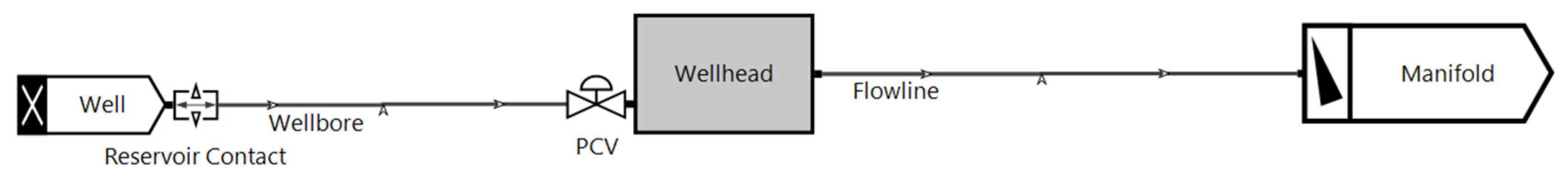
5. Application of OLGA and LedaFlow into Field Case

The real field case detailed in Section 3 is simulated by both LedaFlow and OLGA. This field is characterized by a low production rate. OLGA showed no hydrate blockages during the continuous production stage in the previous study [30]; a notable point of interest is a comparison of how LedaFlow predicts this field case. Two ways to set up the simulations were compared using a steady-state preprocessor and initial condition setup. A guideline about how to initialize the hydrate simulation to get reasonable results will be discussed.

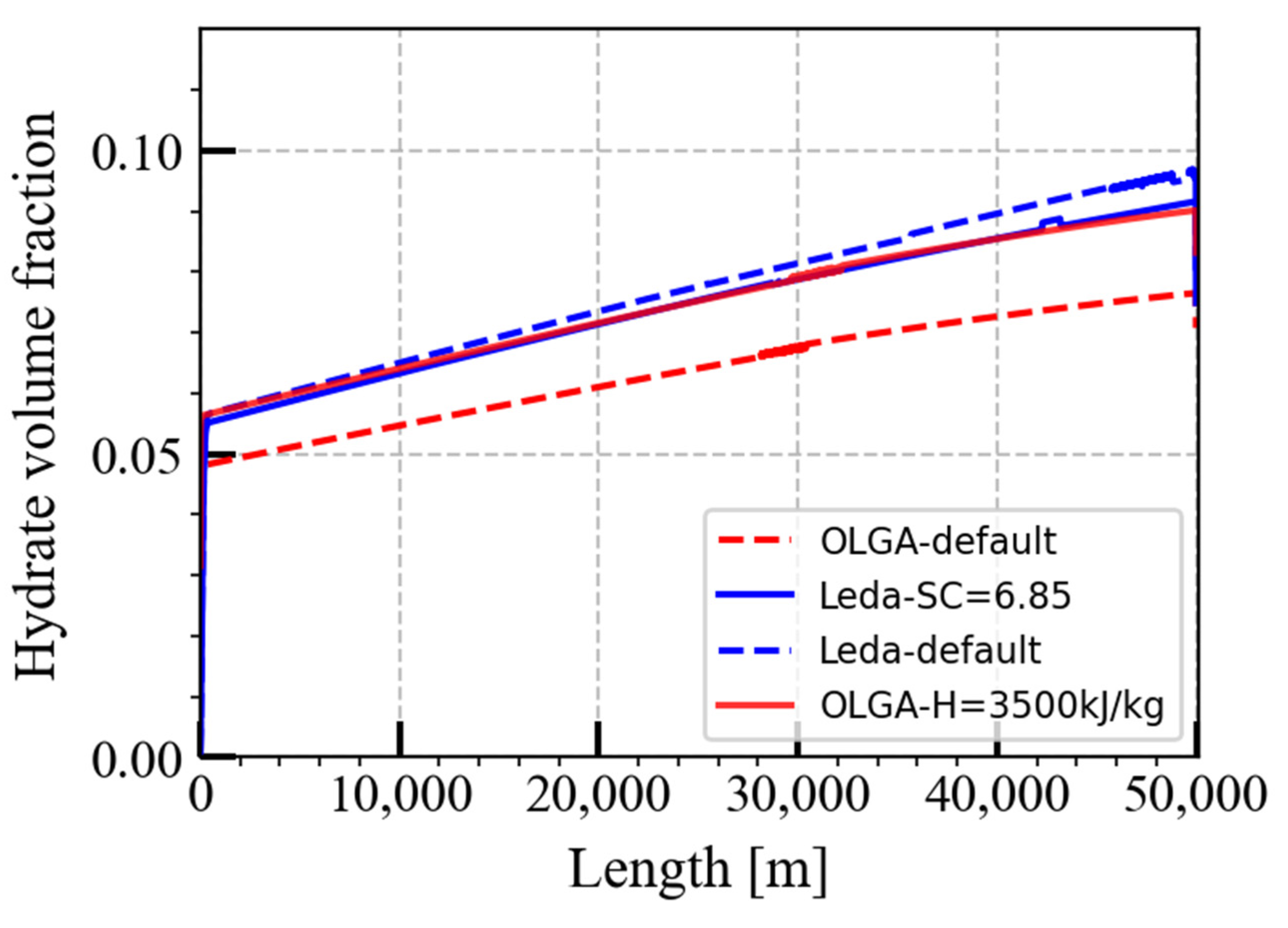
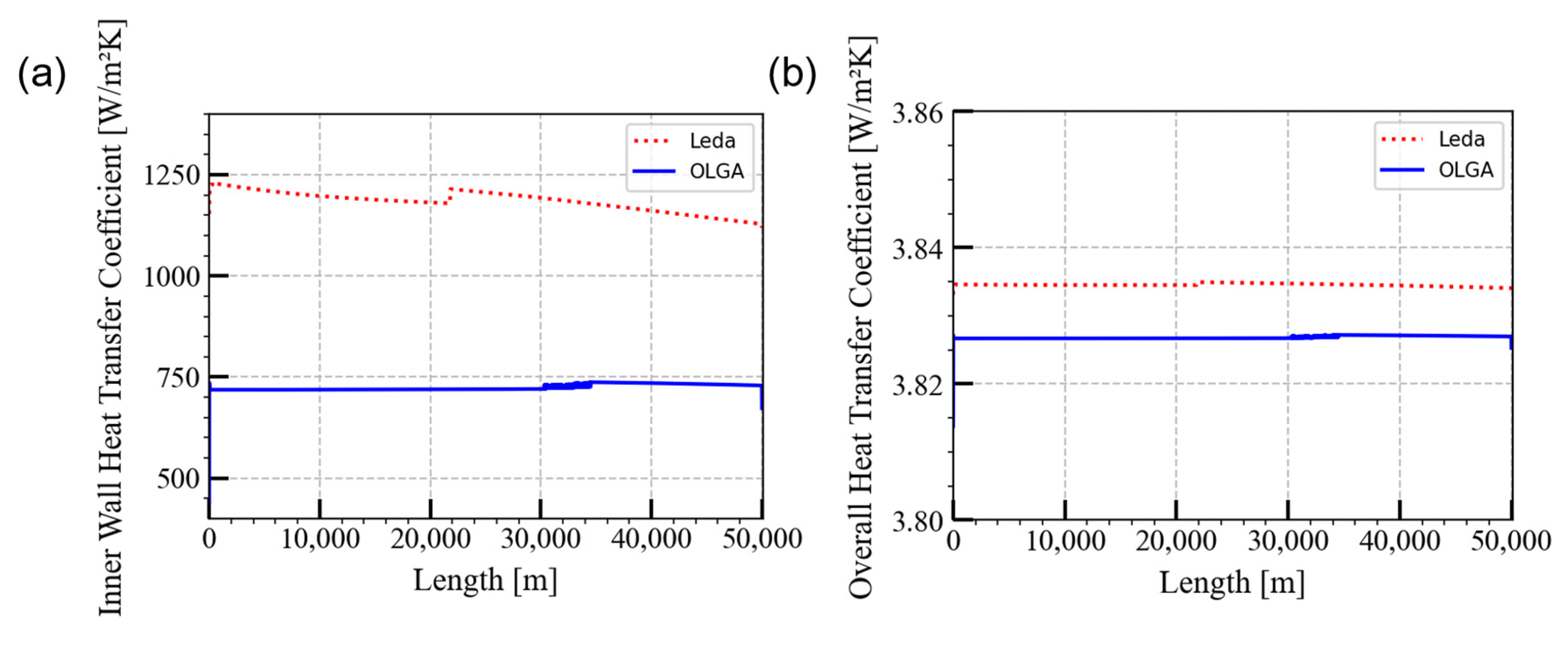
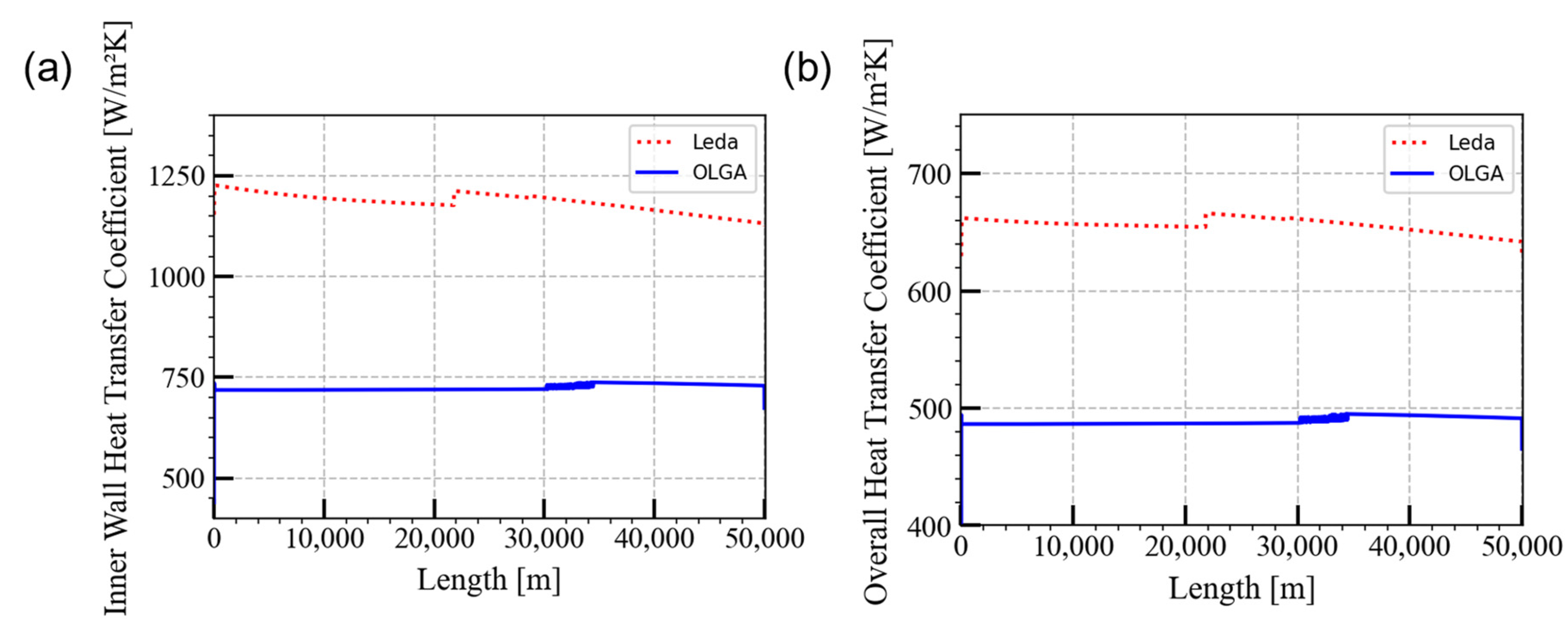
5.1. Steady-State Preprocessor Comparison

Using the steady-state preprocessor is a typical way to initialize the dynamic simulation. In LedaFlow it is based on the point model, which computes the liquid holdup and pressure gradient at each location along the pipe at a steady state. In OLGA, the steady-state preprocessor uses the point model OLGAS THREE-PHASE to find consistent solutions for pressures, temperatures, mass flows, liquid holdups, and flow regimes for flow networks by iteration. Both steady-state preprocessors can be run with hydrate kinetics activated, but they do not consider the formation of hydrates or other flow-assurance solids.

The simulation is first initiated with the steady-state preprocessor with hydrate kinetics inactivated. As shown in Figure 9, at the end of the steady state, the solutions for temperature, pressure, mass flow rate, and volume fraction are very close, except that LedaFlow shows more fluctuations in mass flow rate during the steady-state phase. Given that the geometry of the well pipeline does not have multiple ups and downs, it is inferred that the fluctuation is due to the instability generated by the solver caused by the different point models used.

The field case is then simulated using the steady-state preprocessor with hydrate kinetics activated. In the field simulation setups, key properties of hydrates are adjusted according to the parameter comparison presented in Section 4.2, as shown in

Table 4. Parameters used in OLGA and LedaFlow for field simulation setup.

Parameters	OLGA	LedaFlow
Hydrate distribution phase	Oil (embedded)	Hydrate distribution coefficient (fraction in oil) = 1
Hydration number	6.85 (embedded)	6.85
Enthalpy	3500 kJ/kg gas	477.4 kJ/kg hydrate (embedded)
Kinetics correction factor	0.02	$f_{hydrate}$$=0;f_{water}$ = 10.2
Viscosity model	Camargo and Palermo model: $F_A$$=50\mathrm{mN}/\mathrm{m};f$ = 2.5	SoFA model: $A$$=8.55;X$ = 0.33

, to ensure equivalence between the simulation models.

According to the results shown from both simulators, it was found that using a steady-state preprocessor to define initial conditions can lead to significant numerical issues due to the absence of hydrates in the preprocessor. The initial conditions set by the steady-state preprocessor may include portions of the pipe that are already within the hydrate formation region. When the hydrate model starts, the simulation experiences a high thermal driving force for hydrate formation, potentially causing rapid and excessive hydrate accumulation. This sudden formation of a large amount of hydrates can introduce a discontinuity, disrupting the conservation equations. Such a discontinuity can lead to numerical issues and unrealistic outputs, such as immediate plugging due to the high viscosity of the system. To avoid these problems, it is advisable to use dynamic simulations to achieve a steady state.

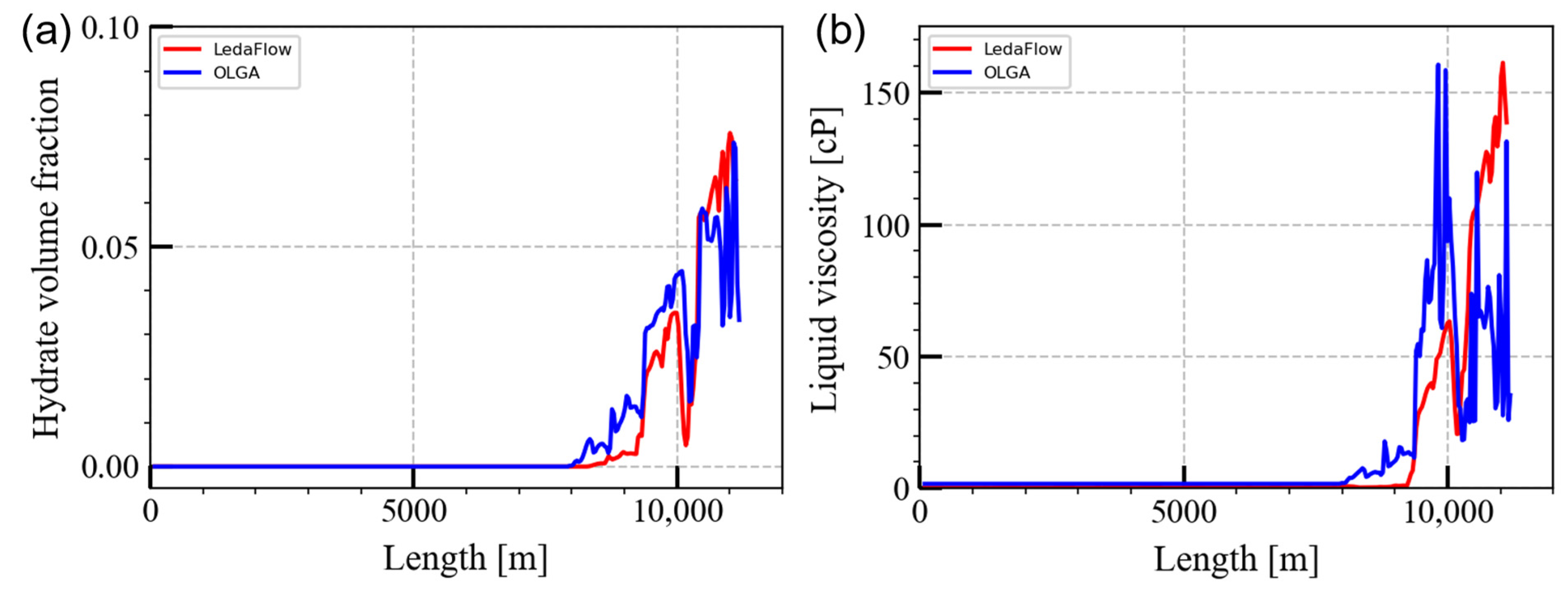
5.2. Initial Condition Comparison

Since preprocessor-initialized conditions can lead to potential numerical issues during modeling, it is recommended to use dynamic simulation to reach the steady state. This approach is similar to scenarios where the system starts from a static condition, such as during well clean-up. This is particularly applicable in hydrate simulation. For example, after an unplanned shut-in event, dead oil displacement can be carried out to minimize the risk of hydrate plugging. Once the dead oil displacement is complete, the initial condition for the subsequent oil production is that the system is filled with static dead oil. Therefore, the user-defined initial conditions can be set to 100% oil holdup, with 0% volume fractions of both gas and water. Using this setup as the initial condition for both the wellbore and the flowline, the well is produced at the desired water cut and flow rate, eventually reaching a steady state through the dynamic simulation. The performance of the hydrate models in OLGA and LedaFlow is then compared using this setup, with the equivalent parameters presented in Table 4. The setup also ensures that water is forced to emulsify in the continuous oil phase in both simulators.

It was found that both OLGA and LedaFlow do not predict hydrate plugs (defined as either a hydrate volume fraction over 50 vol.% or a relative viscosity above 4300) during steady-state production, which aligns with field observations [30]. As shown in Figure 10, both OLGA and LedaFlow predict a maximum hydrate volume fraction of 8 vol.% in the pipeline and a maximum liquid viscosity of around 160 cP. Due to the differences in the base core simulator, as discussed in Section 4.3, it is not expected that the hydrate volume fraction or the viscosity would be exactly equivalent. However, both simulators should provide equivalent conclusions once the simulations are set up based on the same hydrate model presented in this paper.

6. Conclusions

This comparative study of OLGA and LedaFlow for hydrate transport simulations has provided insights into the performance and reliability of each simulator, as well as guidelines for setting up equivalent input parameters for both simulators. The primary focus was on how each simulator handles hydrate formation and plugging in pipelines, which is a critical aspect of flow assurance in the oil and gas industry.

The analysis shows that while both multiphase flow simulators have comparable frameworks, such as their approach to handling conservation equations, discrepancies in hydrate modeling can lead to differing results. Key factors examined in this study include hydrate kinetics, hydrate viscosity, stoichiometric coefficient, and hydrate formation enthalpy. It is recommended that users adjust these parameters based on their understanding of the specific field to achieve more reliable results.

Specifically, the effects of surface area and correction factor on the kinetics model for predicting hydrate volume fraction were investigated. LedaFlow incorporates nucleation prediction, whereas OLGA-CSMHyK does not. Additionally, it was found that heat transfer models are handled differently between OLGA-CSMHyK and LedaFlow. Different results have also been observed when using a steady-state preprocessor, which suggests that a steady-state preprocessor should be avoided during hydrate simulation. It is recommended that the users set appropriate initial conditions to model hydrates. By setting up the initial conditions, hydrates will gradually form to avoid artificial effects. Depending on the simulation conditions, the impact of these factors may vary. Nonetheless, they should be carefully considered for accurate result interpretation when analyzing hydrate formation using OLGA and LedaFlow.

References

1. Chakrabarti, S.K. Handbook of Offshore Engineering; Elsevier: Amsterdam, The Netherlands, 2005; pp. 15–200. [Google Scholar] [CrossRef]
2. Makogon, T.Y. Handbook of Multiphase Flow Assurance; Elsevier: Amsterdam, The Netherlands, 2019; ISBN 9780128130629. [Google Scholar]
3. Sloan, E.D., Jr.; Koh, C.A. Clathrate Hydrates of Natural Gases; CRC Press: Boca Raton, FL, USA, 2007; pp. 1–548. [Google Scholar] [CrossRef]
4. Turner, D.J. Clathrate Hydrate Formation in Water-in-Oil Dispersions. Ph.D. Thesis, Colorado School of Mines, Golden, CO, USA, 2005. [Google Scholar]
5. Camargo, R.; Palermo, T. Rheological Properties of Hydrate Suspensions in an Asphaltenic Crude Oil. In Proceedings of the 4th International Conference on Gas Hydrates, Yokohama, Japan, 9–23 May 2002; pp. 880–885. [Google Scholar]
6. Zerpa, L.E. A Practical Model to Predict Gas Hydrate Formation, Dissociation and Transportability in Oil and Gas Flowlines. Ph.D. Thesis, Colorado School of Mines, Golden, CO, USA, 2013. [Google Scholar]
7. Bassani, C.L.; Barbuto, F.A.A.; Morales, R.E.M.; Cameirão, A.; Herri, J.M.; Sum, A.K. Predicting Gas Hydrate Formation during Three-Phase Gas-(Water-in-Oil) Flow. In Proceedings of the BHR 19th International Conference on Multiphase Production Technology, Cannes, France, 5–7 June 2020; pp. 201–215. [Google Scholar]
8. Bassani, C.L.; Kakitani, C.; Herri, J.M.; Sum, A.K.; Morales, R.E.M.; Cameiraõ, A. A Multiscale Approach for Gas Hydrates Considering Structure, Agglomeration, and Transportability under Multiphase Flow Conditions: III. Agglomeration Model. Ind. Eng. Chem. Res. 2020, 59, 15357–15377. [Google Scholar] [CrossRef]
9. Bhatnagar, G.; Gao, S. Gas Hydrate Management. In Flow Assurance; Gulf Professional Publishing: Cambridge, MA, USA, 2022; ISBN 9780128220108. [Google Scholar]
10. Ballard, L.; Sloan, E.D. The next Generation of Hydrate Prediction IV: A Comparison of Available Hydrate Prediction Programs. Fluid Phase Equilib. 2004, 216, 257–270. [Google Scholar] [CrossRef]
11. Lv, X.; Shi, B.; Wang, Y.; Gong, J. Study on Gas Hydrate Formation and Hydrate Slurry Flow in a Multiphase Transportation System. Energy Fuels 2013, 27, 7294–7302. [Google Scholar] [CrossRef]
12. Zhou, L.; Upchurch, E.R.; Liu, Y.; Anfinsen, B.-T.; Hashemian, Y.; Yuan, Z. Evaluating Subsea Capping Stack Usage for CO2 Blowouts. In Proceedings of the Offshore Technology Conference, Houston, TX, USA, 6–9 May 2024. [Google Scholar] [CrossRef]
13. Qin, H. Hydrate Film Growth and Risk Management in Oil/Gas Pipelines Using Experiments, Simulations, and Machine Learning. Ph.D. Thesis, Colorado School of Mines, Golden, CO, USA, 2020. [Google Scholar]
14. Wang, Y. The Development and Application of Hydrate Formation, Transportation and Bedding Models in Liquid-Dominated Systems. Ph.D. Thesis, Colorado School of Mines, Golden, CO, USA, 2019. [Google Scholar]
15. Kannan, S.N. Modeling and Experiments of Gas Hydrates and Other Solids Management. Ph.D. Thesis, Colorado School of Mines, Golden, CO, USA, 2024. [Google Scholar]
16. Danielson, T.J.; Bansal, K.M.; Hansen, R.; Leporcher, E. LEDA: The next Multiphase Flow Performance Simulator. In Proceedings of the 12th International Conference on Multiphase Production Technology ’05, Barcelona, Spain, 25–27 May 2005; pp. 477–492. [Google Scholar]
17. Puente, P.; Martinez, V.; Richon, V.; Morud, J.; Zambare, N. Wax Deposition and Hydrate Transport Dynamic Simulations on an Oil Pipeline-Experiences Applying Novel Models for Flow Assurance Assessment. In Proceedings of the Society of Petroleum Engineers-Abu Dhabi International Petroleum Exhibition & Conference 2018, ADIPEC 2018, Abu Dhabi, United Arab Emirates, 12–15 November 2018. [Google Scholar] [CrossRef]
18. Giacchetta, G.; Marchetti, B.; Leporini, M.; Terenzi, A.; Dall’Acqua, D.; Capece, L.; Cocci Grifoni, R. Pipeline Wax Deposition Modeling: A Sensitivity Study on Two Commercial Software. Petroleum 2019, 5, 206–213. [Google Scholar] [CrossRef]
19. Leporini, M.; Terenzi, A.; Marchetti, B.; Giacchetta, G.; Corvaro, F. Experiences in Numerical Simulation of Wax Deposition in Oil and Multiphase Pipelines: Theory versus Reality. J. Pet. Sci. Eng. 2019, 174, 997–1008. [Google Scholar] [CrossRef]
20. Belt, R.; Djoric, B.; Kalali, S.; Duret, E.; Larrey, D. Comparison of Commercial Multiphase Flow Simulators with Experimental and Field Databases. In Proceedings of the BHR Group-15th International Conference on Multiphase Production Technology, Cannes, France, 15–17 June 2011; pp. 413–427. [Google Scholar]
21. Akselsen, A.H. Efficient Numerical Methods for Waves in One-Dimensional Two-Phase Pipe Flows. Ph.D. Thesis, Norwegian University of Science and Technology, Trondheim, Norway, 2016. [Google Scholar]
22. OLGA Plugin User Model Numerics and Programmers Guide; Schlumberger: Sagamihara, Japan, 2014.
23. Laux, H. Modeling of Dilute and Dense Dispersed Fluid-Particle Flow. Ph.D. Thesis, Norwegian University of Science and Technology, Trondheim, Norway, 1998. [Google Scholar]
24. Danielson, T.J. Transient Multiphase Flow: Past, Present, and Future with Flow Assurance Perspective. Energy Fuels 2012, 26, 4137–4144. [Google Scholar] [CrossRef]
25. LedaFlow Engineering Version 2.8.264.024-User Manual; Kongsberg Digital: Houston, TX, USA, 2011.
26. Bendiksen, K.; Espedal, M.; Malnes, D. Physical and numerical simulation of dynamic two-phase flow in pipelines with application to existing oil-gas field lines. In Proceedings of the Conference on Multiphase Flow in Industrial Plants, Bologna, Italy, 29–30 September 1988. [Google Scholar]
27. Bendiksen, K.H.; Maines, D.; Moe, R.; Nuland, S. The Dynamic Two-Fluid Model OLGA: Theory and Application. SPE Repr. Ser. 1991, 6, 171–180. [Google Scholar]
28. Beggs, H.D.; Brill, J.P. A Study of Two-Phase Flow in Inclined Pipes. J. Pet. Technol. 1973, 25, 607–617. [Google Scholar] [CrossRef]
29. Wang, Y.; Koh, C.A.; White, J.; Patel, Z.; Zerpa, L.E. Hydrate Formation Management Simulations with Anti-Agglomerants and Thermodynamic Inhibitors in a Subsea Tieback. Fuel 2019, 252, 458–468. [Google Scholar] [CrossRef]
30. Qu, A.; Ravichandran, S.; Hatscher, S.; Ugueto, L.; Torsvik, M.; Zerpa, L.E.; Koh, C. Predicting Hydrate Formation and Plugging in a Gas Condensate Subsea Tieback Using a Transient Hydrate Simulation Tool. In Proceedings of the SPE Annual Technical Conference and Exhibition, San Antonio, TX, USA, 16–18 October 2023. [Google Scholar] [CrossRef]
31. Vysniauskas, A.; Bishnoi, P.R. A Kinetic Study of Methane Hydrate Formation. Chem. Eng. Sci. 1983, 38, 1061–1072. [Google Scholar] [CrossRef]
32. Kalogerakis, N.; Englezos, P.; Dholabhai, P.D. Kinetics of Gas Hydrate Formation from Mixtures of Methane and Ethane. Chem. Eng. Sci. 1987, 42, 2659–2666. [Google Scholar]
33. Boxall, J.; Davies, S.; Koh, C.A.; Sloan, E.D. Predicting When and Where Hydrate Plugs Form in Oil-Dominated Flowlines. SPE Proj. Facil. Constr. 2009, 4, 80–86. [Google Scholar] [CrossRef]
34. Clausse, D.; Gomez, F.; Dalmazzone, C.; Noik, C. A Method for the Characterization of Emulsions, Thermogranulometry: Application to Water-in-Crude Oil Emulsion. J. Colloid Interface Sci. 2005, 287, 694–703. [Google Scholar] [CrossRef] [PubMed]
35. Matthews, P.N.; Notz, P.K.; Widener, M.W.; Prukop, G. Flow Loop Experiments Determine Hydrate Plugging Tendencies in the Field. Ann. N. Y. Acad. Sci. 2000, 912, 330–338. [Google Scholar] [CrossRef]
36. Boxall, J.A. Hydrate Plug Formation from <50% Water Content Water-in-Oil Emulsions. Ph.D. Thesis, Colorado School of Mines, Golden, CO, USA, 2009. [Google Scholar]
37. Palermo, T.; Tournis, E. Viscosity Prediction of Waxy Oils: Suspension of Fractal Aggregates (SoFA) Model. Ind. Eng. Chem. Res. 2015, 54, 4526–4534. [Google Scholar] [CrossRef]
38. Muhle, K. Floc Stability in Laminar and Turbulent Flow. In Coagulation and Flocculation: Theory and Applications (Surfactant Science Book 47); CRC Press: New York, NY, USA, 1993; pp. 355–390. [Google Scholar]
39. Mills, P. Non-Newtonian Behaviour of Flocculated Suspensions. J. Phys. Lett. Edp Sci. 1985, 46, 301–309. [Google Scholar] [CrossRef]
40. Potanin, A.A. On the Mechanism of Aggregation in the Shear Flow of Suspensions. J. Colloid Interface Sci. 1991, 145, 140–157. [Google Scholar] [CrossRef]
Figure 1. Conceptual picture showing major hydrate plugging mechanisms in an oil-dominated system, Figure from Turner [4], modified from [6].
Energies 17 06101 g001
Figure 2. Schematic of real field setup.
Energies 17 06101 g002
Figure 3. (a) Bathymetry of the subsea tieback of the well and flowline connecting the well and the following manifold and (b) detailed geometry of the flowline. Reproduced and modified from [30].
Energies 17 06101 g003
Figure 4. (a) An example hydrate equilibrium curve and data points taken for gas consumption rate calculation as shown in (b). (b) Hydrate reaction rate with respect to subcooling from LedaFlow with different tuning factors and CSMHyK.
Energies 17 06101 g004
Figure 5. Relative viscosity at different hydrate volume fractions given by C&P and SoFA models with different parameter setups.
Energies 17 06101 g005
Figure 6. Hydrate volume fraction from LedaFlow and OLGA with default setups and tuned reaction heat ( H ) or hydration number (SC). The red dashed line represents OLGA results using the default setup with the H = 4100 kJ/kg and SC = 6.85. The blue dashed line represents LedaFlow results with H = 477.4 kJ/kg and SC = 4.8. The blue solid line shows LedaFlow results with the default H = 477.4 kJ/kg and tuned SC of 6.85, while the red solid line shows OLGA results with the default SC of 4.8 and a tuned H = 3500 kJ/kg.
Energies 17 06101 g006
Figure 7. (a) Inner wall heat transfer coefficient, and (b) overall heat transfer coefficient profile of the horizontal pipeline in OLGA/LedaFlow when h i is significantly greater than h o .
Energies 17 06101 g007
Figure 8. (a) Inner wall heat transfer coefficient, and (b) overall heat transfer coefficient profile of the horizontal pipeline in OLGA/LedaFlow when h i and h o are in a similar order of magnitude.
Energies 17 06101 g008
Figure 9. Mass flow rate from OLGA and LedaFlow in the well of the field case without hydrate formation, with the well elevation shown on the right vertical axis.
Energies 17 06101 g009
Figure 10. (a) Hydrate volume fraction and (b) liquid viscosity along the pipeline length from LedaFlow and OLGA using initial condition setup.
Energies 17 06101 g010