Abstract
This paper examines Connected Smart Green Townhouses (CSGTs) as a modern residential building model in Burnaby, British Columbia (BC). This model incorporates a wide range of sustainable materials and smart components such as recycled insulation, Photovoltaic (PV) solar panels, smart meters, and high-efficiency systems. The CSGTs operate in grid-connected mode to balance on-site renewables with grid resources to improve efficiency, cost-effectiveness, and sustainability. Real datasets are used to optimize resource consumption, including electricity, gas, and water. Renewable Energy Sources (RESs), such as PV systems, are integrated with smart grid technology. This creates an effective framework for managing energy consumption. The accuracy, efficiency, emissions, and cost are metrics used to evaluate CSGT performance. CSGTs with one to four bedrooms are investigated considering water systems and party walls. A deep Machine Learning (ML) model combining Long Short-Term Memory (LSTM) and a Convolutional Neural Network (CNN) is proposed to improve the performance. In particular, the Mean Absolute Percentage Error (MAPE) is below 5%, the Root Mean Square Error (RMSE) and Mean Absolute Error (MAE) are within acceptable levels, and is consistently above 0.85. The proposed model outperforms other models such as Linear Regression (LR), CNN, LSTM, Random Forest (RF), and Gradient Boosting (GB) for all bedroom configurations.
1. Introduction
Resource optimization in Smart Buildings (SBs) has advanced significantly with a focus on efficiency, performance, and cost reduction while minimizing emissions [1,2,3,4,5]. Integrating Renewable Energy Sources (RES), such as Photovoltaic (PV) systems, is essential for sustainable energy use in cities. Predictive analytics and supportive energy policies also play vital roles in SB optimization [6,7,8]. Studies show that Smart Grid (SG) integration can lower costs, reduce emissions, and enhance building performance [9,10,11]. Connected Smart Green Buildings (CSGBs) aim to increase resource efficiency and sustainability. They utilize advanced technologies and RES to achieve economic and environmental benefits [12,13,14].
Buildings contribute significantly to energy use and emissions. For instance, the U.S. building sector accounted for 32% of primary energy use in 2019, with similar trends in other countries [15,16,17]. Improving efficiency is crucial for lowering Greenhouse Gases (GHGs) and costs. In the EU, a 20% increase in building efficiency can save around 60 billion Euros annually [18]. Managing energy use in buildings can help address climate change. There is a need for advanced Heating, Ventilation, and Air Conditioning (HVAC) systems and predictive energy strategies to improve SB efficiency [19,20,21]. Data-driven energy management systems can further optimize energy use.
Machine Learning (ML) and predictive analytics enable real-time control and adaptability for SBs [22] to increase efficiency, lower emissions, and provide accurate energy predictions. ML-based models such as Long Short-Term Memory (LSTM) and Convolutional Neural Networks (CNN) can improve energy management in grid-connected buildings [19,20,21,22]. This paper introduces a deep hybrid LSTM-CNN model for resource optimization in CSGBs. This model improves resource use and aligns with sustainability goals. Cross-sector collaboration is key to advancing sustainable practices for CSGBs. The focus here is on optimizing energy use in grid-connected CSGBs [23,24].
2. CSGT Modeling
This section presents the CGST model, emphasizing effective technology-driven solutions. SGBs provide a sustainable architecture by merging advanced technology with eco-friendly design [25]. Energy modeling is essential in sustainable construction as it helps predict building performance and balance resource efficiency with environmental goals while prioritizing occupant well-being.
Grid connectivity is a key aspect of this work as it enables dynamic energy optimization by utilizing real-time data from the grid for better load balancing and demand response. This mode integrates RESs like PV systems with the grid to ensure a stable supply when RESs are insufficient. It enhances operational efficiency by allowing for the sale of excess renewable energy and optimization based on time-of-use pricing. The grid-connected model also supports scalability, providing a foundation for smart communities with microgrids and energy hubs.
2.1. Climate
This paper considers the energy and climate challenges in Canada, focusing on the unique environment of Burnaby, British Columbia (BC). The impact on load consumption and energy optimization in smart and green buildings is examined. Understanding the climate is crucial for designing SGTs [22,26,27,28].
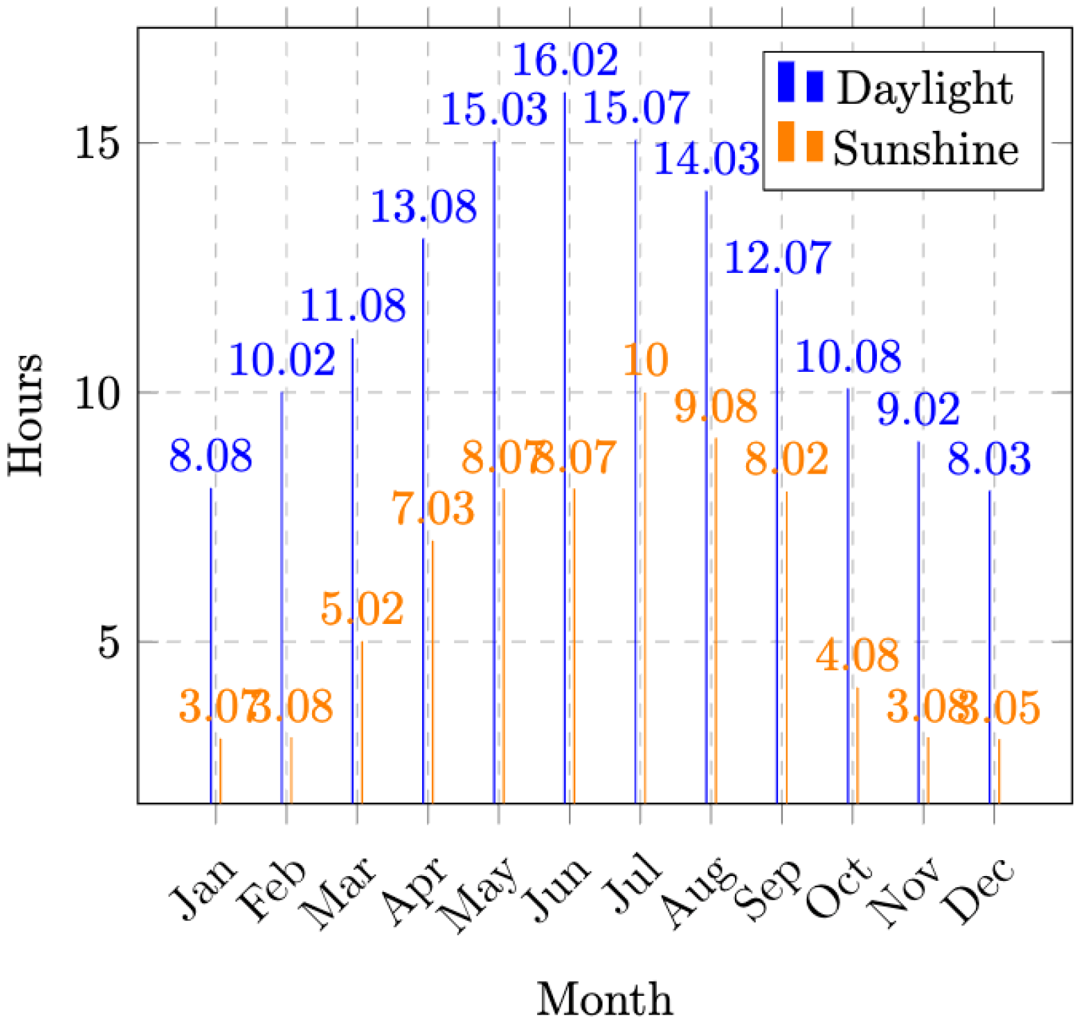
Figure 1 gives the average daylight hours (blue bars), which is the time from sunrise to sunset each month. This shows how long the sun is above the horizon, regardless of the weather. Also given are the sunshine hours (orange bars), which are the actual hours of sunlight without obstruction. These hours are typically less than daylight hours due to clouds or rain. Figure 1 indicates that maximum daylight occurs in June with 16.02 h, and the minimum occurs in December with 8.03 h.

Figure 1.
Average daylight and sunshine in Burnaby [28] during January to December 2023.
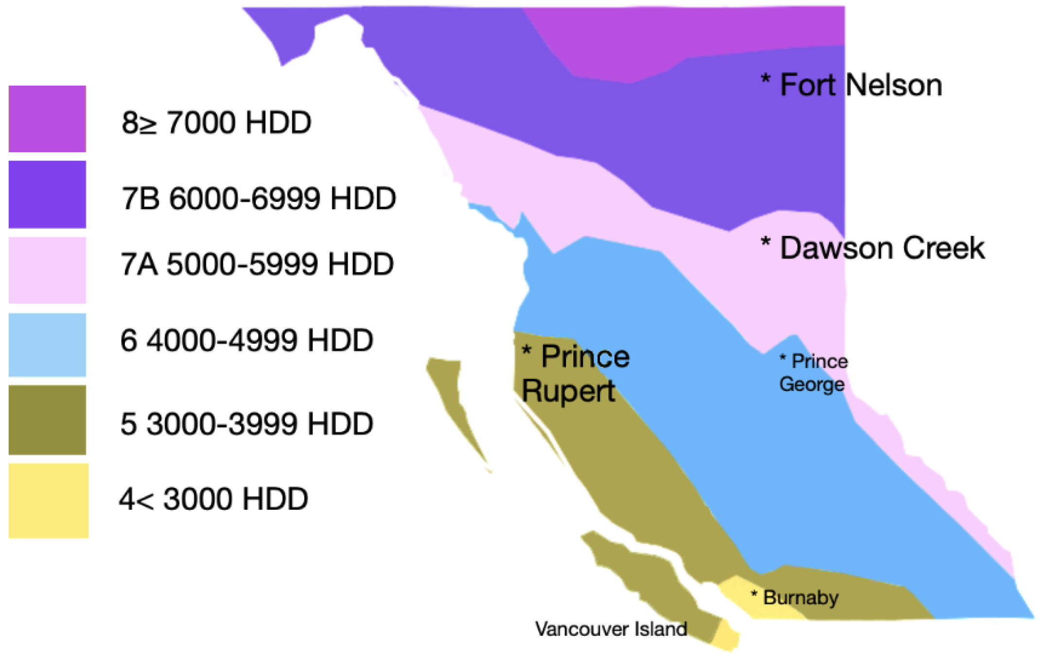
Heating Degree Days (HDD) are used to estimate the energy needed to heat buildings based on outdoor temperatures. HDD measures how much and for how long the outdoor temperature is below 18 C, indicating when heating is needed. The unit is C · days. Architects and engineers use HDD to design heating systems and improve resource efficiency. Utilities use HDD to predict heating fuel demand and manage supply. By understanding HDD trends, energy use can be optimized, reducing emissions and enhancing sustainability. Figure 2 shows the climate zones in BC based on HDD, which are crucial for climatic analysis. HDD provides vital data for designing efficient heating systems in the proposed SGTs.
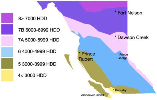
Figure 2.
BC climate zones based on Heating Degree Days (HDD) [13].
2.2. SGT Formulation
This work considers a characteristic home from [25,29,30], with slight modifications for a one-story townhouse in Burnaby. The base model is a two-story townhouse (2140 sq ft) built in 1995 and renovated in 2007–2008 [25]. Major renovations typically occur every 15–20 years. The home is oriented south to enhance resource efficiency. The one-Bd SGT is for a young couple in their 30s without children. The two-Bd SGT is for a couple in their late 30s with one child. The three-Bd SGT is for a couple in their early 40s with two teenage children. The four-Bd SGT is for a mature couple in their mid-40s with a family of five.
Leadership in Energy and Environmental Design (LEED) certification and Canada Green Building Council (CGBC) standards are crucial for resource efficiency and emission reduction [25]. The approach focuses on limiting emissions by using electricity as the sole energy source and installing PV systems for net-zero energy [31]. This eliminates on-site fossil fuel usage. Surplus electricity can be exported to neighbors during sunnier months. Neighbors with their own PV systems may also generate excess energy, particularly during peak sunlight hours.
Table 1 lists the sustainable materials and components used for SGTs in Canada [21]. Each is selected for its eco-friendly properties and contribution to sustainable living. Many are already widely used in sustainable buildings globally. Bamboo flooring is renewable, durable, and aesthetically appealing. Recycled and reclaimed wood are commonly used for structural and decorative purposes, promoting waste reduction and resource conservation. PV panels, LED lighting, and heat pumps are essential for energy-efficient buildings and are employed in residential and commercial buildings and GBs [32,33,34]. They meet local and international codes for sustainability, resource efficiency, fire safety, and structural integrity [35,36,37], including LEED and Building Research Establishment Environmental Assessment Method (BREEAM) standards.

Table 1.
The sustainable materials and components of SGTs.
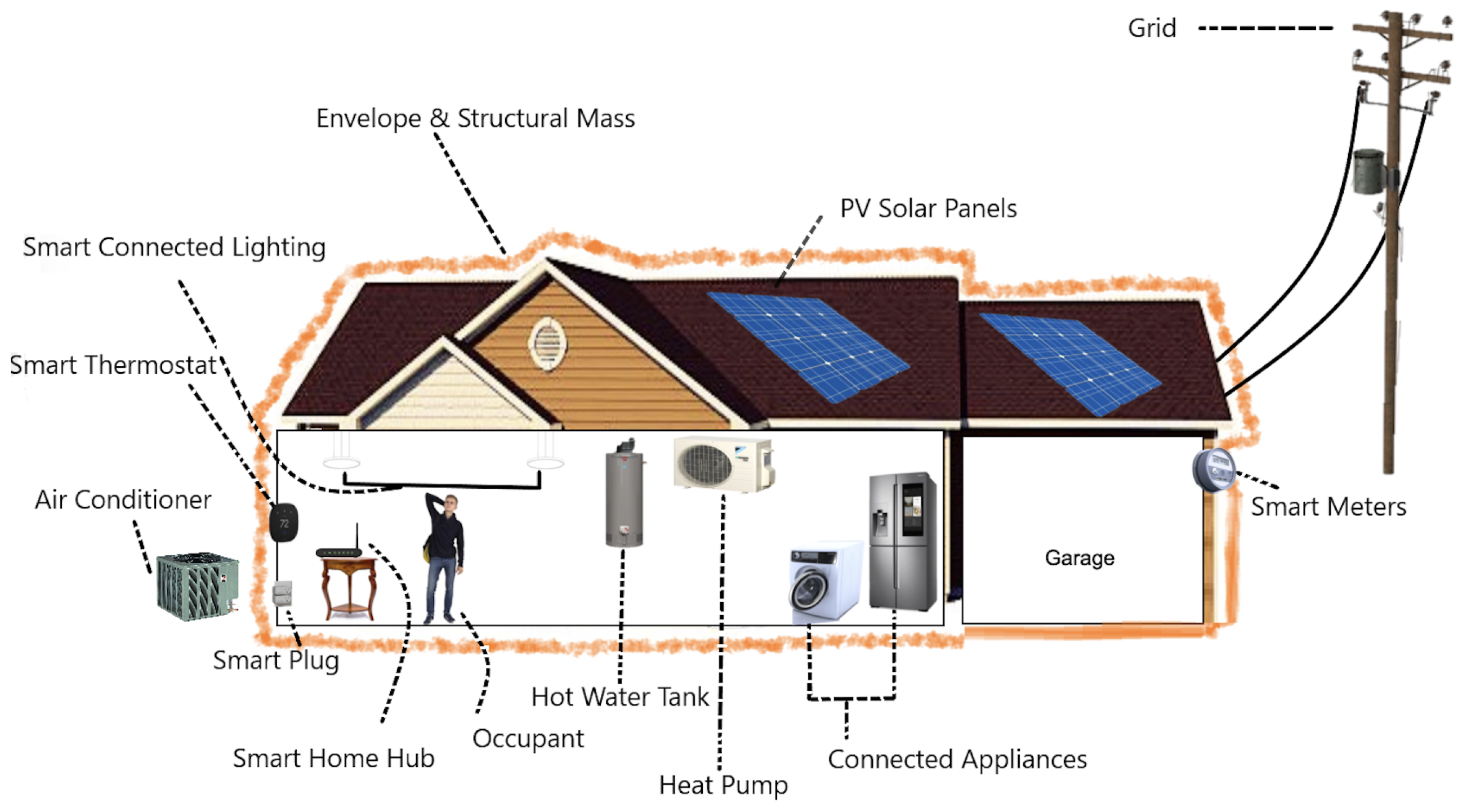
Having both air conditioners and heat pumps in SGB designs ensures efficient temperature control year-round, saving energy and reducing environmental impact [38,39]. Heat pumps transfer heat rather than generate it, making them more energy-efficient than traditional heating systems. They can provide both heating and cooling, reducing the need for separate systems. As heat pumps use electricity, they help reduce GHG emissions. High-efficiency air conditioners are better suited for extreme cooling needs. Modern air conditioners, especially those connected to smart systems, allow remote control and optimized cooling cycles for energy reduction [38,39]. This work considers R6 windows that reduce heat transfer and improve insulation, thus lowering energy consumption for heating and cooling [21]. This conforms with R2000, a Canadian energy efficiency standard [40]. Figure 3 shows the SGT components in grid-connected mode. An HVAC system performance model based on [20,40,41] is employed here.

Figure 3.
SGT components in grid-connected mode.
2.2.1. Connecting Townhouses for Improved SGTs
Connecting residential buildings reduces resource consumption and costs [42]. This is crucial in SGTs to lower load consumption, lower costs, and improve efficiency. Connected buildings enable more efficient energy management [42] as they form a single unit similar to Micro-Grids (MGs) [43,44]. CSGTs in grid-connected mode are considered to reduce electricity consumption, improve demand response, and enhance overall performance. The building consists of four connected townhouses (one-, two-, three-, and four-bedroom CSGTs). Grid connection adds to the system complexity. In this work, the challenges and solutions related to load consumption in SGTs connected to the grid are examined [42]. The advantages of connecting SGTs include reduced resource consumption, lower costs, improved efficiency, and load optimization. These benefits demonstrate how connected systems contribute to sustainable and efficient SGBs.
Real datasets for connected townhouses include two key components: connected water systems [25,45] and party walls [46,47]. Party walls are shared walls between adjacent properties and are commonly found in townhouses. They are jointly owned and maintained by property owners. Agreements for party walls outline the responsibilities for maintenance, repairs, alterations, and dispute resolution. Connected townhouses depend on these walls for structural integrity, noise reduction, fire safety, and boundary responsibilities. Connected water systems are also crucial for building performance and occupant comfort [45]. This work investigates the operational aspects of district cooling systems in connected buildings [45]. These systems distribute chilled water to multiple buildings, which improves resource efficiency. Resource consumption, temperature management, and system efficiency are examined, as well as how building operations impact cooling infrastructure performance.
2.2.2. CGST Formulation
The CGST formulation is based on the results in [48,49]. The heat transfer is given by
where Q is the heat transfer rate, k is the thermal conductivity of the wall material, A is the surface area of the wall, is the temperature difference across the wall, and d is the thickness of the wall. This expression describes conductive heat transfer, where thermal energy moves through a solid material. The heat transfer rate is proportional to the thermal conductivity of the material and the cross-sectional area through which the heat moves. It also depends on the temperature difference across the material. However, the rate is inversely proportional to the thickness of the material. This is important for designing energy-efficient systems such as insulation in buildings.
The continuity is
and indicates that the rate of change of mass within the volume is equal to the difference between the mass flow rate entering and leaving the system. This is used to analyze fluid behavior in pipes, ducts, and other systems.
The resource consumption is given by
and is the sum of the consumptions across different components, systems, or time periods. The goal is to optimize the conditions, such as temperature settings and flow rates, to minimize consumption while maintaining comfortable temperature levels and ensuring adequate flow rates.
The building energy balance is
where Energy In is the total resource consumption and PV output. This includes electricity (lighting, HVAC), gas, and water use. PV output is part of Energy In as it reduces the need for external energy. Energy Out consists of heat loss, heat gain, and total resource consumption output. Heat loss occurs through walls, windows, and the building envelope, while heat gain is the reverse. Total resource consumption output includes energy used by internal systems like HVAC, lighting, and appliances. Energy Storage refers to changes in energy storage within the building, both internally and externally.
Renewable Energy Integration (REI) refers to the incorporation of RES into the building energy system
where Renewable Energy Used is the energy derived from renewable sources like PV panels, and Total Energy Consumption is the resources consumed by the building. This provides a quantitative measure of how much of the building resource consumption is being met by RESs. A higher REI indicates a greater reliance on RES. This is desirable to reduce the carbon footprint and achieve sustainability goals.
The Smart Technology Utilization Index (STUI) is a metric used to quantify the effectiveness and efficiency of smart technology implementation in a building and is given by
where Number of Smart Devices is the number of smart devices used in the building and Total Devices is the number of devices in the building.
Table 2 gives a detailed breakdown of the specifications for the SGTs, ranging from a base townhouse with one bedroom (Base) to a large townhouse with four bedrooms (four-Bd). It provides parameters such as bedroom sizes, living spaces, and total area. Table 3 summarizes the key energy system parameters for the SGTs. Water heating demand is the energy required for daily hot water use (kWh/day) and varies with the number of bedrooms and expected water consumption. HVAC system capacity is the required HVAC capacity (kW) to maintain indoor comfort and varies by townhouse size and layout. PV panel capacity is the installed capacity (kW) of the PV panels. These data are used in OpenStudio to evaluate energy performance and optimize the design for energy-efficient GBs.

Table 2.
The SGT specifications.

Table 3.
OpenStudio SGT specifications for water heating demand, HVAC capacity, and PV panel capacity.
Accurate resource consumption modeling depends on the floor plan, building size, and height, as in Figure 4 and Table 2. Floor plans show the building layout, including bedrooms, kitchen, living room, bathrooms, and storage. Building size and height reflect the volume and capacity of the building, which affect energy needs for heating, cooling, and ventilation. Townhouse sizes are measured in square feet (sq ft).
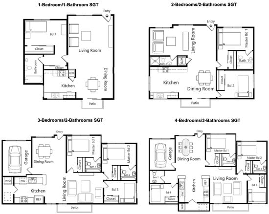
Figure 4.
One to four bedroom SGT floor plans.
2.3. Experimental Setup
This work employs data collection and software tools to create and test models. Data collection involves building, resource consumption, and weather data. These were gathered through sensors placed within the building. OpenStudio 3.8.0 was used for energy simulation by creating virtual building models for resource consumption scenarios and efficiency solutions. Python 3.11.5 [50] was used for energy optimization, with pandas for data manipulation, NumPy [51] for numerical calculation, and Matplotlib [52] for visualization. The Ninja [53] website was used to analyze and compare PV systems [54,55]. The building model was created in OpenStudio 3.8.0, which integrates with EnergyPlus. OpenStudio automatically converts the .osm file into an EnergyPlus input file (.idf) for execution. The CSGT results were generated using Python and EnergyPlus. Python interfaces with EnergyPlus through the pyenergyplus library. This facilitates simulation automation and the extraction of performance data.
Experiments were conducted to validate the models. Four different townhouse sizes were analyzed to evaluate energy performance, efficiency, and sustainability. Energy performance measures the balance between resources consumed and generated for heating, cooling, lighting, and appliances. Different townhouse sizes cater to various family needs. The models were trained on historical data and validated against real-world observations. Cross-validation was employed to ensure robust solutions.
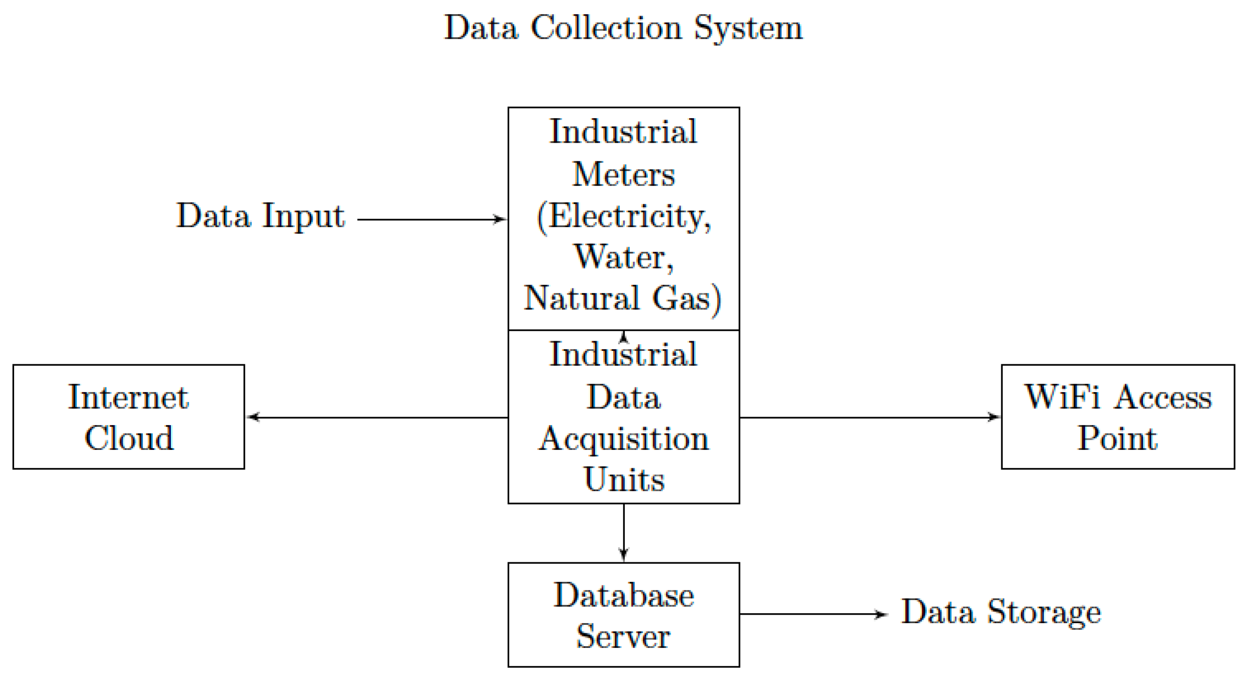
Real datasets from [25,29,37,38,39] are used for modeling. Scripts for converting database tables into datasets were obtained from these references. The AMPds2 dataset is openly available via Harvard Dataverse in CSV, tab-delimited, and RData formats [25,29,30,37]. The data collection system shown in Figure 5 monitors resources such as electricity, water, and gas. Data are collected from meters and sent to data acquisition units, which transmit it to a central server. A WiFi access point and cloud connection allow for remote access and integration of external data, enabling real-time monitoring to optimize resource management [22,26,27,37]. A Building Management System (BMS) is not necessary due to the moderate size of the building network, the simplicity of energy optimization, and the ability to refine strategies through monitoring and assessment. Industrial meters are used for their precision, durability, and reliability. They easily integrate with data acquisition systems for real-time analysis and are suitable for monitoring multiple resources in complex networks like connected townhouses.
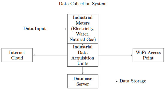
Figure 5.
Block diagram of the data collection system.
Assessing the efficiency, performance, and accuracy of PV panels is key to optimizing RE generation in sustainable housing. Table 4 provides PV panel parameters for different SGT sizes. A 1 kW system produces about 1200 kWh/year, assuming 1200 h of effective sunlight and 15% cell efficiency. SGT production is calculated by multiplying capacity (in kW) by 1200 kWh/kW/year. Thus, the one-Bd SGT (2.56 kW) produces 3072 kWh/year, the two-Bd (3.21 kW) produces 3840 kWh/year, the three-Bd (3.84 kW) produces 4608 kWh/year, and the four-Bd (4.48 kW) produces 5376 kWh/year. The payback period is calculated based on energy savings.

Table 4.
PV panel parameters for different SGT sizes.
The total installation cost is
and the annual energy savings is
Then, the payback period for the one-Bd SGT (2.56 kW) is 12.4 years, the two-Bd SGT (3.21 kW) is 15.5 years, the three-Bd SGT (3.84 kW) is 18.6 years, and the four-Bd SGT (4.48 kW) is 21.6 years. These results provide insights into the financial investment and energy savings for SGTs, which help assess their economic viability.
2.4. SGT Performance Metrics
This section presents the key metrics for evaluating and improving the resource efficiency, performance, emissions, and cost of SGTs. The Total Energy Use Intensity (TEUI) is
where Total Energy Consumption is the sum of all energy in kWh and Total Building Area is the floor area in sq ft. This gives an energy efficiency measure per unit area [56]. The Total Energy Demand Intensity (TEDI) is
where Total Energy Demand is the peak demand in kW and Total Building Area is the floor area in sq ft. A lower TEDI indicates better resource efficiency.
The Energy Consumption Based on Size of Home (SOH) is
where k is a constant factor to normalize the relationship between the total area of the home and energy consumption intensity. Energy Consumption Intensity is the average rate of resource consumption per unit area. The Control Efficiency Index (CEI) is
where AEU is the actual resource consumption and OEU is the optimal energy usage under ideal conditions. The CEI is used to identify inefficiencies in control strategies.
The Waste Recycling Rate (WRR) is
where Weight of Recycled Waste (WRW) is the total recycled waste weight and Total Weight of Waste is the total weight of the waste generated. A higher WRR indicates better recycling performance. The Material Recycling Percentage (MRP) is
where WRM is the recycled material weight, and TWMU is the total weight of the material used.
The Indoor Air Quality (IAQ) Index is
where IAQ Measurement is the quantitative assessment of indoor air quality parameters such as CO2, VOCs, CO, and O3 [57].
The Seasonal Energy Efficiency Ratio (SEER) is
where the EER values are the efficiencies for different cooling capacities. The Energy Efficiency Ratio (EER) is
where BTU denotes British thermal unit, which is a unit of energy used to measure heat, and W is the power consumption of the system in watts. The Heating Seasonal Performance Factor (HSPF) is
The Coefficient of Performance (COP) is
where Q is the useful heat output and W is the work input required.
The Water Efficiency is
where Water Saved is the amount of water saved by efficiency measures and Total Water Used is the total amount of water consumed.
The Electrical Consumption Efficiency (ECE) is
where Useful Electrical Output is the total electrical energy used by the system and Electrical Input includes energy losses. The Gas Consumption Efficiency (GCE) is
where Heat Output is the useful heat energy from gas and Gas Input is the total gas consumed.
The R-value is a measure of the thermal resistance of a material, indicating how well it resists the flow of heat. It is used to indicate the insulation properties of a material, with higher values indicating better insulation [58]. The R-value of insulation material (in ft2F·hr/BTU) is
d is the thickness of the insulation material (in inches), and k is the thermal conductivity of the material (in BTU·in/(ft2F·hr)). This value is used to represent the thermal resistance of building components such as walls, windows, roofs, and floors, which contribute to the overall thermal efficiency of the building envelope and thus impact energy performance. OpenStudio allows R-values to be input for components to analyze thermal performance. Key R-values include exterior walls (R-30), windows (R-5, triple-pane with low-emissivity coatings), roof/ceiling (R-50), and floor/slab (R-20, to reduce heat loss through the foundation). OpenStudio provides detailed thermal metrics based on the specified materials and their properties.
The carbon footprint of building operations, expressed in kgCO2, is
It includes CO2, CH4, and N2O emissions converted into CO2 equivalents. The floor area of the building is in sq ft [59]. Regulatory compliance with code standards, including TEUI, TEDI, and GHGI thresholds, is critical. Meeting or exceeding these benchmarks shows environmental leadership [59]. Buildings with favorable TEUI, TEDI, and GHGI ratings attract more investment, improving long-term viability and economic value [59]. Incorporating these into building design and management improves resource use and reduces environmental impact. It also enhances building resilience [59].
A cost analysis helps evaluate resource consumption savings, Return on Investment (ROI), and overall cost–benefit. This is vital for assessing the economic feasibility of efficiency measures and sustainability goals [60]. The cost of energy is
where Total Energy Consumption is the total resources consumed by the building and Unit Cost is the cost of energy in kWh. Cost savings are the financial savings achieved by comparing costs before and after efficiency measures are implemented
where Cost Before is the cost incurred before implementing resource efficiency initiatives and Cost After is the cost after their implementation. The ROI assesses the financial return on the investment made and is given by
where Net Savings is the total savings achieved from resource efficiency measures and Initial Investment is the cost of implementing these measures. The Net Benefit is the overall financial benefit and is given by
where Total Savings is the cumulative savings achieved from resource efficiency initiatives and Total Costs is the total cost of implementing and maintaining these measures.
The HVAC metric is defined as
where is the ith parameter value, and are the corresponding maximum and minimum values, and n is the number of parameters. The parameters included in this metric are heat transfer efficiency, fluid dynamics efficiency, building energy balance, TEUI, TEDI, cooling energy consumption, and IAQ.
Table 5 presents the outcomes for water systems and party wall connections in the SGTs. These results are for grid-connected mode and include daily hot water usage, energy savings, PV panel output, and HVAC system usage. This shows that the daily hot water usage increases with the number of bedrooms, from 58.9 gallons for the one-Bd SGT to 128.6 gallons for the four-Bd SGT. The energy savings from shared walls improve with townhouse size, from 8.2% in the one-Bd unit to 18.1% in the four-Bd unit. The PV panel output increases with unit size from 6.8 kWh for the one-Bd unit to 11.9 kWh for the four-Bd unit. HVAC system usage slightly decreases with shared walls, from 1.32 tons for the one-Bd unit to 2.74 tons for the four-Bd unit. One ton is 12,000 BTU/hour of cooling capacity. As the number of bedrooms increases, resource usage and energy output also increase. Shared walls, however, yield significant energy savings. Comparing Table 3 and Table 5 indicates the improvements in efficiency and resource use with shared infrastructure in CSGTs. These units benefit from better energy management, reduced costs, and greater sustainability. The results in Table 3 and Table 5 show that CSGTs perform better in several key areas. Shared walls reduce total resource consumption. PV panel output indicates effective solar resource use, and HVAC usage is lower than the capacity in Table 3, reflecting better energy management. Daily hot water use is also optimized in connected SGTs. Thus, CSGTs provide clear improvements in resource efficiency, solar utilization, and HVAC usage.

Table 5.
Outcomes related to water systems and party wall construction in connected SGTs.
3. Methodology
A goal of this work is to investigate the relationships among parameters impacting smart and green technologies [61,62]. A hybrid model combining CNN and LSTM networks is considered to optimize SGTs. It was shown in [63] that hybrid models can outperform other approaches. CNNs can effectively identify spatial features and detect patterns in environmental and energy data. LSTM networks capture temporal dependencies, enabling accurate prediction of resource consumption. A hybrid CNN-LSTM-AE model was developed in [64] for energy prediction. The CNN extracts features that are input to the LSTM encoder, and then the LSTM decoder generates the final prediction results. This model has lower Mean Square Error (MSE), Mean Absolute Error (MAE), Root Mean Square Error (RMSE), and Mean Absolute Percentage Error (MAPE) compared with other models for data from UCI residential and Korean commercial buildings. Thus, it is more effective in energy optimization. In [65], a CNN-LSTM model was used for indoor temperature modeling of HVAC systems. Traditional methods lack long-term accuracy due to data noise and nonlinearity. The CNN-LSTM model combines the feature extraction of convolutional layers with the sequential learning of LSTM. This hybrid model is more accurate than MLP or LSTM and thus addresses the limitations of traditional ML approaches.
3.1. The Proposed SGT Algorithm
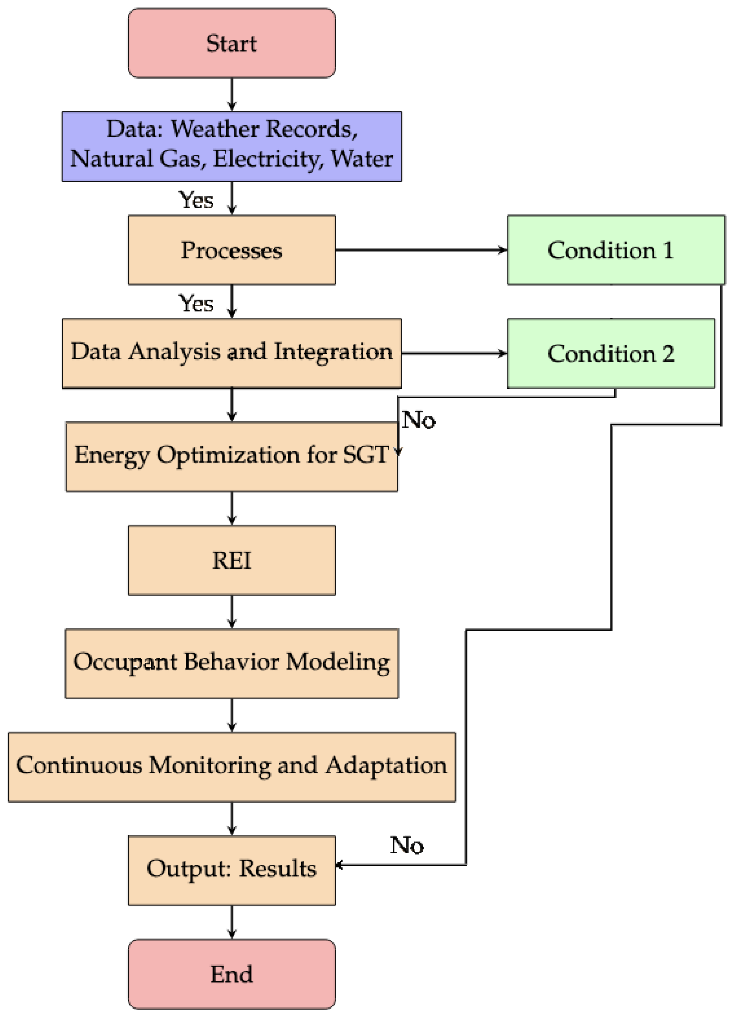
This section outlines the proposed ML algorithm. The goal is to optimize resource efficiency, reduce the environmental impact, and improve building performance. A hybrid model combining CNN and LSTM networks is employed [50,51,65]. This model can capture both spatial and temporal dependencies in SGT data. Figure 6 presents a flowchart of the proposed model, including data analysis, SB control, RE integration, occupant behavior modeling, and continuous monitoring. The flowchart steps are as follows:
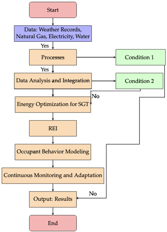
Figure 6.
Flowchart of the proposed SGT algorithm.
- Start: process initiation.
- Data input: weather, gas, electricity, and water data.
- Preprocessing: data cleaning, transformation, and normalization.
- Data Analysis and Integration: insights and patterns are obtained.
- Condition 1: check the analyzed data. If the outcome is yes, proceed to energy optimization; otherwise, go to Output.
- Energy Optimization: implement the energy optimization.
- Condition 2: evaluate the optimization results. If the outcome is yes, proceed to RE Integration; otherwise, go to Occupant Behavior Modeling.
- RE Integration (REI): add RES into the energy optimization.
- Occupant Behavior Modeling: model occupant influence on energy.
- Continuous Monitoring and Adaptation: monitor the parameters and adjust strategies based on occupant behavior and energy use.
- Occupant Behavior Modeling: incorporate routines, seasonality, and usage trends. Daily routines are more active in the morning (6–8 AM) and evening (6–10 PM). Seasonal variations include winter heating and summer cooling. Working hours are lower on weekends and more predictable on weekdays. There are more special events during holidays and fewer during vacations. Working from home increases daytime activity and resource use. Temperature, lighting, and smart appliance use vary by occupant. These factors influence energy use patterns and thus SGT efficiency.
- Output: results provide optimized energy usage, cost savings, and recommendations.
- End: process conclusion.
3.2. Optimization
The proposed deep hybrid LSTM-CNN model addresses two key optimization goals.
- Energy Optimization: minimize the prediction errors (e.g., MAE and RMSE) to reduce energy use and improve system efficiency.
- ML Model Optimization: refine the LSTM-CNN model to provide better prediction accuracy. Iterative training is employed to adjust the weights and biases to improve energy forecasting.
This dual focus provides optimized energy management and model performance.
The objectives are as follows:
- Cost Reduction
- Energy optimization for efficient scheduling and operation of energy systems to lower costs (e.g., electricity, fuel, and maintenance).
- ML model optimization for accurate predictions to support cost-effective energy decisions.
- Emission Reduction
- Energy optimization for forecasts to help decrease reliance on non-RESs, lowering carbon emissions.
- ML model optimization for predictions for optimal RES integration to reduce emissions.
- Performance Improvement
- Energy optimization to ensure an reliable energy supply to efficiently meet demands.
- ML model optimization to improve prediction accuracy, which aids effective system management.
- Efficiency Improvement
- Energy optimization to reduce waste and improve energy system resource utilization.
- ML model optimization to increase computational efficiency for faster, more accurate predictions.
The objective function is
where C is cost (minimize), E is emissions (minimize), P is performance (maximize), and is efficiency (maximize). The factors are set based on the importance of each component. Historical data are used to compare and prioritize these objectives. The coefficients used for the objective function are as follows:
- indicates moderate emphasis on minimizing cost, as reducing expenses is important but must be balanced with other factors.
- indicates lower weight on emission reductions as they are considered to have lower priority than cost.
- indicates the highest weight is on performance improvement, which reflects a focus on maximizing system performance.
- indicates the lowest weight, so efficiency is not a critical factor.
The optimization problem has the following constraints:
Energy In includes local generation and grid imports, while Energy Out includes both consumed energy and exports to the grid. Energy Storage is the energy held within the system. These constraints ensure solutions adhere to practical limits and regulations. According to the International Electrotechnical Commission (IEC) 62933 standard for electrical energy storage systems, Energy Storage should be between 10% and 90% of the total capacity [66]. These constraints ensure compliance with building codes and sustainability standards, which is crucial for practical deployment. They also support system stability and performance to balance energy use, cost, and environmental impact.
The following limitations must be considered to ensure suitable solutions:
- Predefined Minimum or Maximum Values: some variables have strict minimum or maximum limits. For example, thermostat settings may range from 18 C to 25 C, and battery storage capacity is limited to 10–90% to extend battery life.
- Computational Limits: computational resources and time constraints may restrict the complexity and scalability of the optimization approach.
- Real-world Constraints: budgetary and regulatory requirements can affect the optimization.
An ML algorithm is employed to predict and optimize resource use to improve sustainability in SGTs and CSGTs. Artificial Neural Networks (ANNs) are powerful tools for SB modeling and energy optimization [67]. They are effective in load forecasting, optimization, occupancy prediction, anomaly detection, and energy optimization [68,69,70,71]. A rule-based approach to predict unusual load conditions, such as on public holidays, was introduced in [68]. These conditions are challenging due to their infrequency and unique patterns. The approach used combines expert insights with statistical models such as Holt-Winters-Taylor exponential smoothing and Auto-Regressive Moving Average (ARMA) to predict both regular and unusual load patterns. Evaluation of this approach using nine years of half-hourly load data for Great Britain showed accurate forecasts up to a day ahead.
The Short-Term Load Forecasting (STLF) model is
where is the forecast load at time t, are the historical load data and relevant features up to time t, and f is the prediction function learned by the NN. STLF feature selection using Random Forest (RF) was presented in [69]. This method was used with 243 features from historical data and time information. Then an enhanced sequential backward search based on permutation importance was used to identify an optimal subset of features. This subset is used to train the RF model. This approach achieved higher accuracy than methods such as support vector regression and ANN.
The predicted occupancy at time t is
where , , and are the corresponding time, day, and weather features, are the past occupancy data, and g is the prediction function learned by the NN. The hybrid energy prediction method for SG in [70] uses STLF and k-medoid clustering to group transformers by energy profiles to speed up training. The deep NN model has six layers and uses Adam optimization. This approach improves scalability and reduces training time by 44% with no loss in accuracy.
Anomaly detection finds deviations from normal behavior based on historical data. The anomaly score at time t is
where h is the NN function. ANNs have been shown to provide excellent energy optimization results. In [72], an ANN-based predictor was developed to forecast daily HVAC power use. This LSTM-based approach has low error and high correlation with test data, which indicates effective real-time prediction. The accuracy is better than with simple one-hour-ahead models.
HVAC optimization involves minimizing energy use under comfort constraints
where is the energy cost at time t and is the corresponding HVAC control input such as temperature. Comfort constraints ensure thermal comfort within buildings. These constraints influence HVAC optimization by penalizing deviations from desired temperature or humidity set-points.
The system dynamics describe HVAC system behavior over time in response to inputs and disturbances, often modeled using physics-based equations or simulation. ML models like LSTM capture these dynamics through time-series forecasting from historical data. Operational limits define boundaries to ensure efficient and safe system performance. ML models enforce these limits with constraints or penalty terms, ensuring control inputs do not exceed predefined operational ranges. It has been shown that ANNs provide excellent accuracy, efficiency, and performance for building energy optimization and handle nonlinearities and dynamic environments better than traditional methods.
3.3. The Proposed Hybrid ML Model
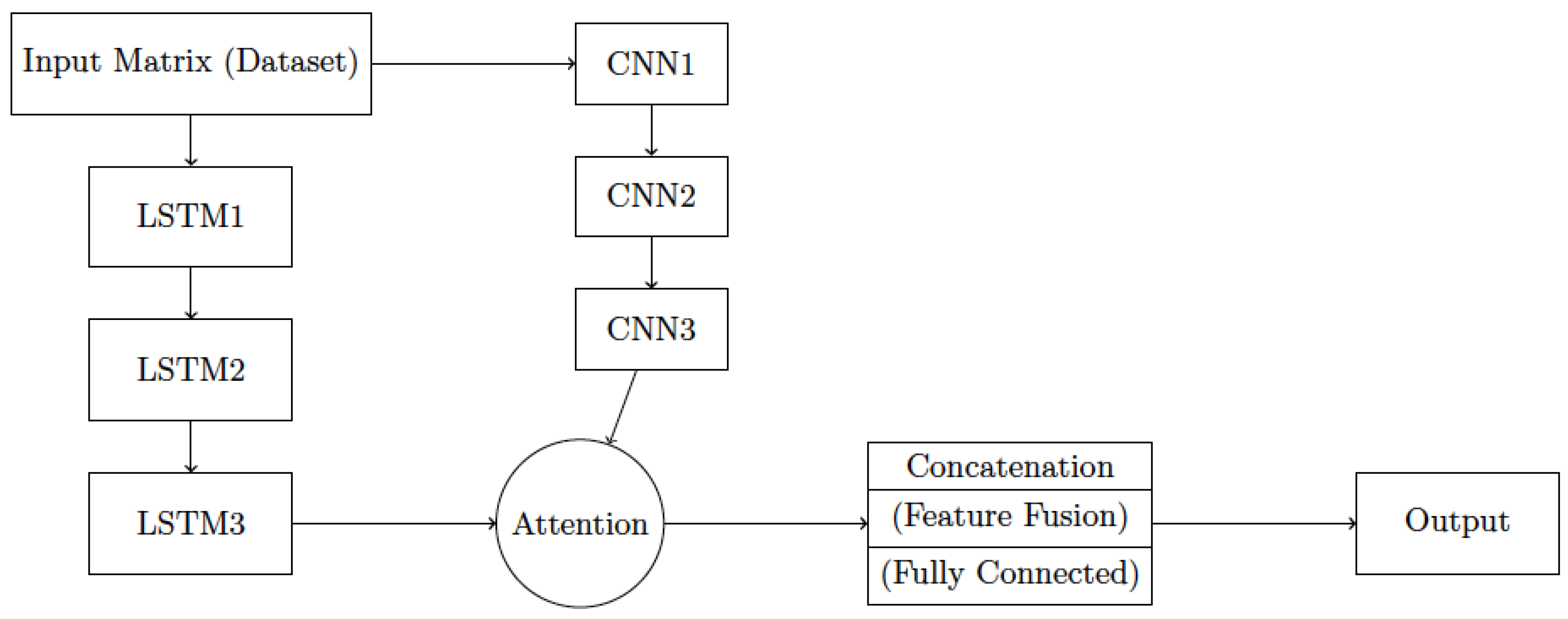
This section describes the architecture of the proposed hybrid ML model, which is illustrated in Figure 7. This model captures both temporal dependencies and spatial patterns in data through the integration of LSTM. The architecture is described below:
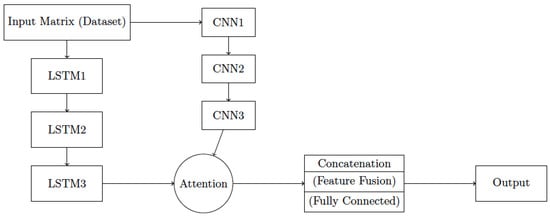
Figure 7.
The proposed deep ML model architecture.
- Input Matrix (Dataset): the input data are loaded in matrix format.
- LSTM Layers with Attention Mechanisms [73]: the LSTM1, LSTM2, and LSTM3 layers use attention mechanisms to focus on relevant parts of the input. This helps capture long-term dependencies and improve prediction accuracy.
- CNN Layers with Skip Connections: the CNN1, CNN2, and CNN3 layers have skip connections that allow information to flow directly between the LSTM and CNN layers. This enable simultaneous capture of spatial and temporal features.
- Attention Mechanism: combines the LSTM and CNN outputs by weighting them based on relevance. This improves the ability of the model to capture both sequential and spatial aspects of the data.
- Concatenation (Feature Fusion and Fully Connected: the LSTM, CNN, and attention features are concatenated and processed through a fully connected layer. This generates fused features for predictions.
- Output: the output layer generates predictions based on the processed features to obtain resource consumption patterns in SBs.
The proposed model combines LSTM layers with attention mechanisms and CNN layers with skip connections to capture long-term dependencies and hierarchical spatial features, respectively. This hybrid architecture is specifically designed for energy optimization in SGTs to achieve resource efficiency, cost savings, and emission reductions. The attention mechanisms and skip connections create more informative features to learn rich, hierarchical representations that improve model generalization ability. The attention mechanisms also allow the model to adapt to varying input conditions. It handles different sequence lengths and complexities, which makes the model more robust and versatile. Skip connections help prevent the vanishing gradient problem and speed up training.
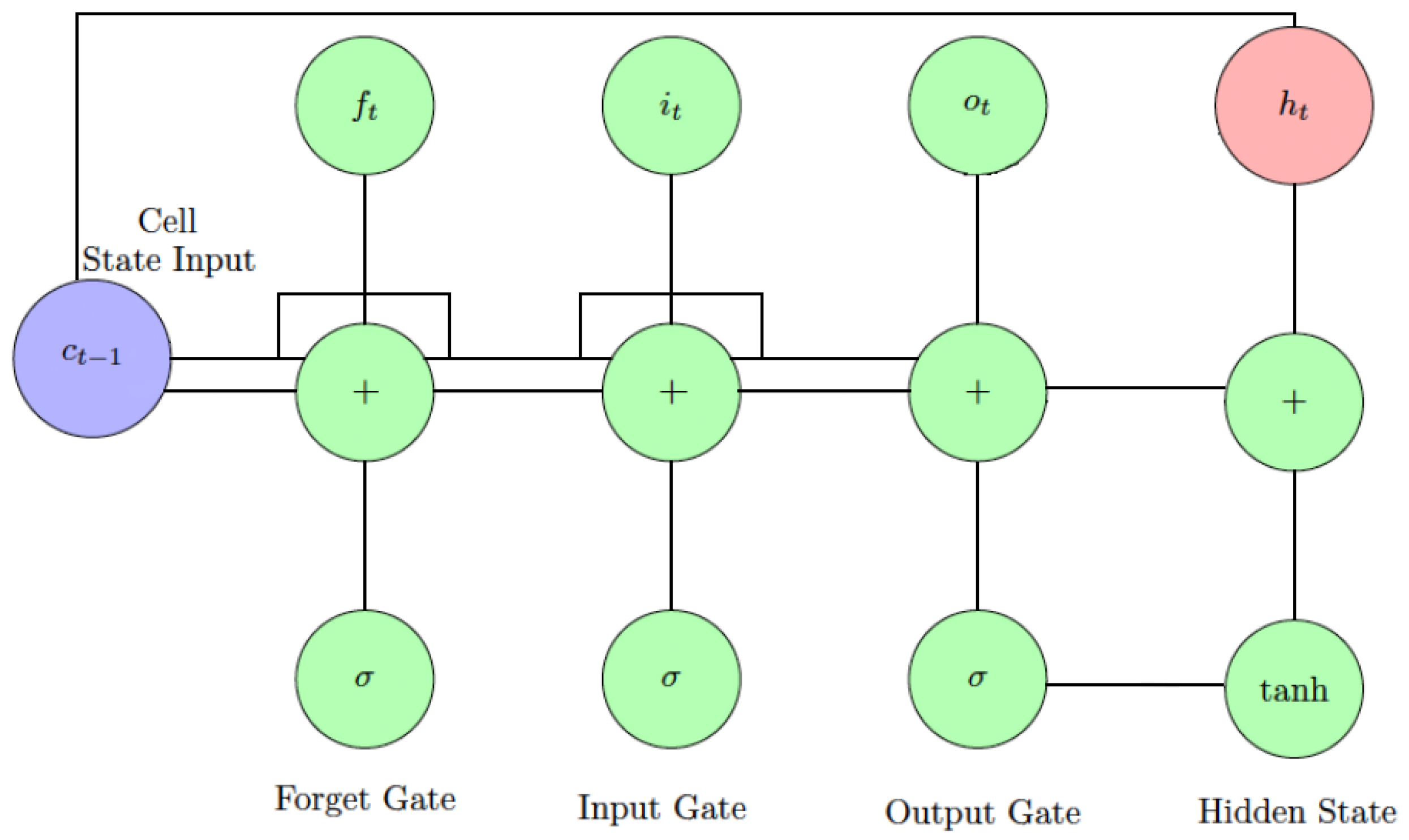
Figure 8 illustrates the Peephole LSTM unit. It is a type of RNN used in sequence modeling tasks. The input node (blue circle) is the input to the LSTM unit at time step t. The forget, input, and output gates (green circles) control information flow. Each gate uses a sigmoid function to output values between 0 and 1. The forget gate decides what to discard, the input gate determines what to store, and the output gate controls information flow to the output. The hidden state (red circle), denoted , is the output of the LSTM at time step t. The cell state (purple circle), denoted , is the internal memory of the LSTM and is updated based on the gate outputs. The previous cell state is used to calculate the new cell state.
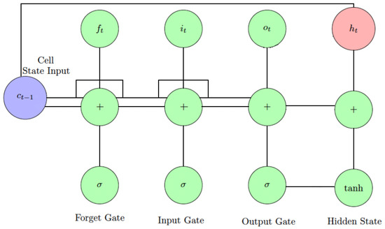
Figure 8.
The Peephole LSTM unit.
A flowchart of the data processing is given in Figure 9. This ensures data cleanliness and relevance for accurate energy optimization predictions. The steps are described below:
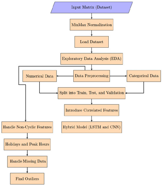
Figure 9.
The data processing flowchart.
- Input Matrix (Dataset): the dataset is loaded. It contains features and target variables for energy optimization. The features include the following:
- −
- Timestamp: day and month.
- −
- Weather data: temperature, humidity, wind speed, and solar radiation.
- −
- Building characteristics: size, rooms, and window sizes.
- −
- Energy consumption history: usage at different intervals.
- −
- Occupancy: number of occupants.
- −
- External factors: energy prices and grid signals.
- −
- Categorical data: appliance types, holidays, and peak hours.
The target variables include resource consumption at different time intervals. Data sources include IoT sensors, external weather services, and historical energy usage databases. - Min-Max Normalization: the input data are scaled to the range [0, 1] to ensure equal contribution from all features.
- Load Dataset: the dataset is loaded for processing.
- Exploratory Data Analysis (EDA): statistical analysis, pattern identification, and data visualization to understand the structure and issues like missing values or outliers.
- Data Preprocessing: cleaning the data, handling missing values, encoding categorical variables, and scaling features to prepare for model training.
- Split into Train, Test, and Validation: the data are divided into subsets for model training, evaluation, and hyperparameter tuning.
- Cross-Validation: partition the dataset into K folds (e.g., 5-fold) for cross-validation. In each iteration, one fold is reserved for validation, while the remaining folds are used for training. Then each fold trains and validates the LSTM-CNN model on a unique split, ensuring robust evaluation by exposing the model to varied data subsets. The results are averaged across all K folds to reduce overfitting and improve generalization.
- Introduce Correlated Features: add correlated features to improve model performance.
- Handle Non-Cyclic Features: separate processing is used for non-cyclic features such as month, day, and hour.
- Holidays and Peak Hours: holidays and peak hours (6–9 AM and 4–9 PM) are added as features for better prediction accuracy.
- Handle Missing Data: missing data points are imputed or removed to avoid bias in predictions.
- Find Outliers: outliers are identified and handled to prevent skewed predictions.
The data are normalized using Min-Max normalization [74] given by
where is the tth original value and and are the maximum and minimum values, respectively.
The feature vector is
where L is the past load values, H is the hour of the day (time-based variations), D is the day of the week (daily usage patterns), M is the month (seasonal variations), is the holiday indicator (binary/categorical), is the weather data (e.g., temperature, humidity), is the spatial features (e.g., building size, occupants), is the start-up patterns (e.g., peak times), and is the appliance usage data (aggregated power consumption). These nine features contain both temporal and spatial patterns in load data and serve as inputs to the ML model.
4. Results and Discussion
This section presents the model performance, including prediction accuracy, efficiency, cost savings, emission reductions, and overall system effectiveness. Base, SGT, and CSGT results are compared. All townhouses are assumed to be connected to the Burnaby electricity grid managed by BC Hydro, operating at 120/240V single-phase for residential connections.
4.1. Resource Optimization
The resource optimization was evaluated for SGTs connected to the Burnaby grid. The availability of RES affects the energy mix and carbon footprint. The weather parameters from 2012–2014 include heating and cooling thresholds at 14 C and 20 C, respectively. The heating power required is 0.3 kW/ C, and the cooling power is 0.15 kW/C. The smoothing rate is 0.5 , solar gain is 0.012 C in W/m2, and wind chill is −0.2 C in W/m2. Parameters such as TEUI, TEDI, and GHGI reflect how climate affects resource consumption and emissions. The average annual temperature is 11.5 C, with summer highs of 23.5 C and winter lows of 1.5 C.
Equations (1)–(36) were implemented using Python and EnergyPlus with the pyenergyplus library to obtain the parameters given in Table 6. The building model was created in OpenStudio, which integrates with EnergyPlus. The cost of energy is in Canadian dollars (CAD). The base home design was adapted to one, two, three, and four bedroom SGTs while maintaining the same location and energy supplies. The key observations from this table are as follows:

Table 6.
Monthly energy performance for the SGTs versus the CSGTs without an ML model.
- Improved party wall insulation increased heat transfer efficiency by 5%.
- Reduced air leakage improved fluid dynamics by 3%.
- Better temperature regulation reduced resource consumption by 9%.
- Energy balance improved by 3% with thermal regulation.
- Control integration provided a 1% improvement.
- TEUI and TEDI decreased by 5% due to shared systems.
- HVAC performance improved by 2% with shared systems.
- Connected systems contribute up to a 1% improvement in water efficiency depending on the building size and optimized management further improves this, resulting in a total improvement of up to 3%.
Considering resource efficiency, CSGTs have 6–10% lower resource consumption per square foot, with better HVAC efficiency (3–5%). The environmental impact is improved as CSGTs reduce GHGI by 5–8% and provide a 10–12% improvement in REI, indicating superior use of RESs. CSGTs show a 3–5% improvement in ROI due to better RE integration and resource efficiency, making them more cost-effective. CSGTs outperform SGTs in energy balance and water efficiency, with improvements of 3–6%. This reinforces that connected systems optimize resource use and improve overall performance. The results in Table 6 confirm that CSGTs provide superior resource efficiency, environmental impact, and cost-effectiveness, supporting their preference for sustainable urban development.
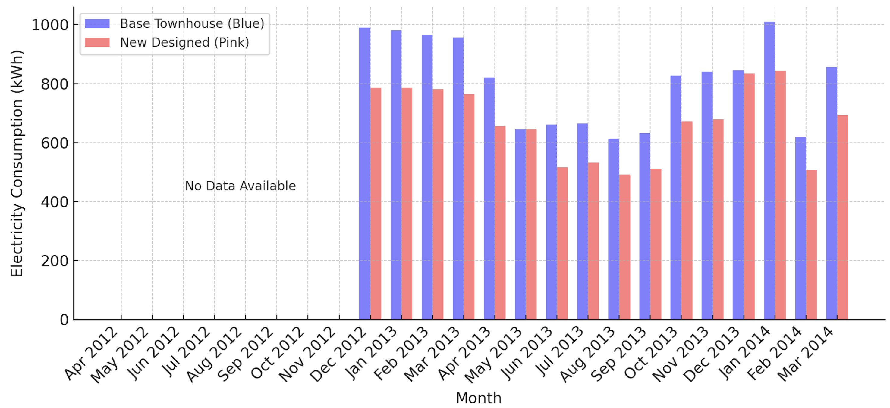
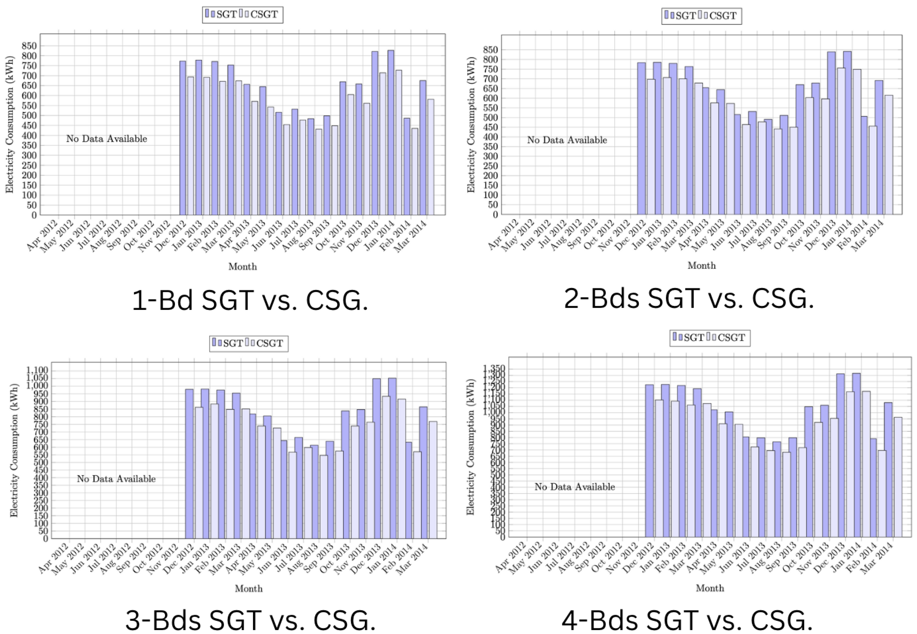
Figure 10 compares monthly electricity consumption between a two-story townhouse dataset from [25] (blue) and a new one-story base townhouse (red) over 2012–2014. The bars show electricity consumption for each month, illustrating the differences between the two designs. Figure 11 presents the monthly electricity consumption (2012–2014) for one to four bedroom SGTs and CSGTs in grid-connected mode. This shows that CSGTs (light blue) consume less electricity than SGTs (dark blue) in most months. The connected features in CSGTs reduce consumption, especially in December 2012 and January–February 2013. This is because energy-saving features such as improved HVAC and lighting controls are more effective during colder months. The townhouse in [25] consumes 120 GJ of gas annually, while the one-story SGT uses only 80 GJ. This represents a 33% reduction, or 40 GJ, in gas consumption. The reduction is mainly due to the energy-efficient features of the SGT. Shared energy optimization strategies further reduce gas usage for heating and other purposes throughout the year.
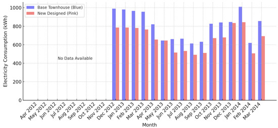
Figure 10.
Monthly electricity consumption (2012–2014) for a new one-story townhouse (pink) and the base townhouse from [25] (blue).
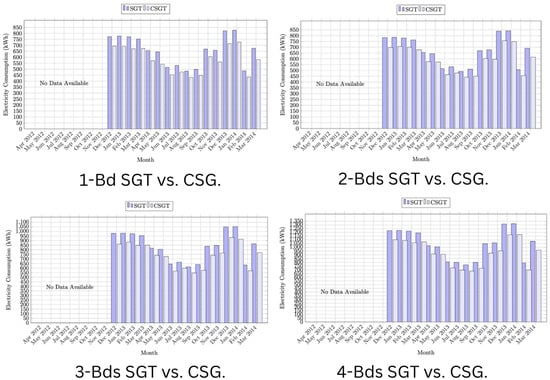
Figure 11.
Monthly electricity consumption (2012–2014) For one to four Bd SGTs and CSGTs in grid-connected mode.
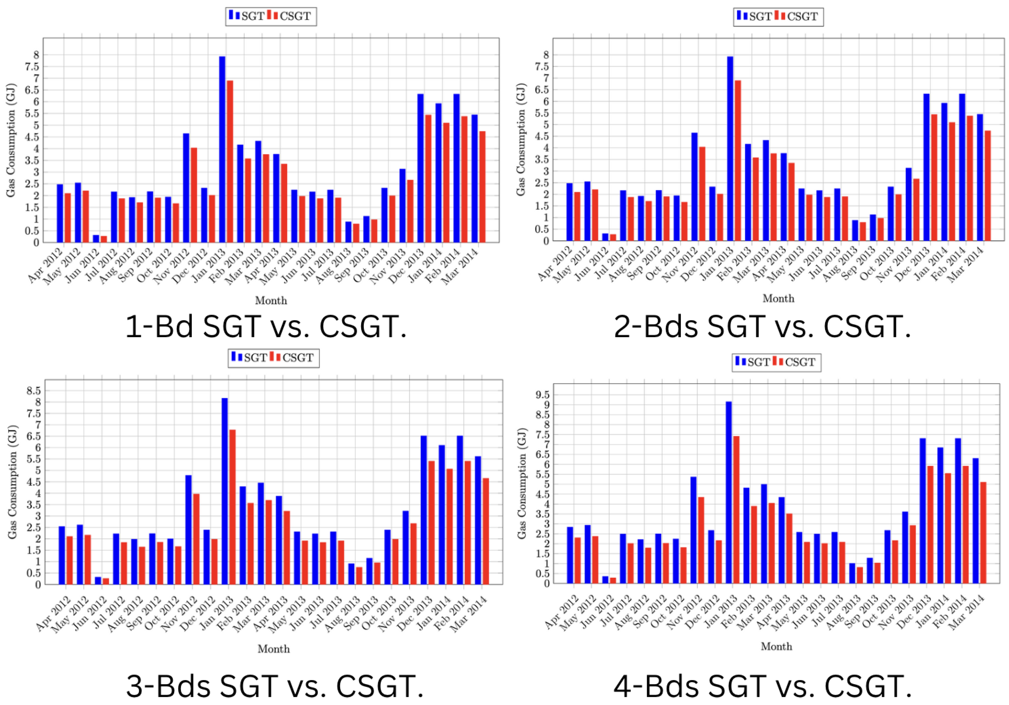
Figure 12 gives the gas consumption of SGTs and CSGTs in grid-connected mode. The one-Bd CSGT uses 13–15% less gas annually than the one-Bd SGT. The two-Bd CSGT consumes 16–17% less gas than the two-Bd SGT. For the three-Bd CSGT, gas consumption is 20–21% lower than the three-Bd SGT. The four-Bd CSGT shows an 18–19% reduction compared with the four-Bd SGT. These results highlight the superior energy efficiency of CSGTs and their potential for sustainable residential energy use.
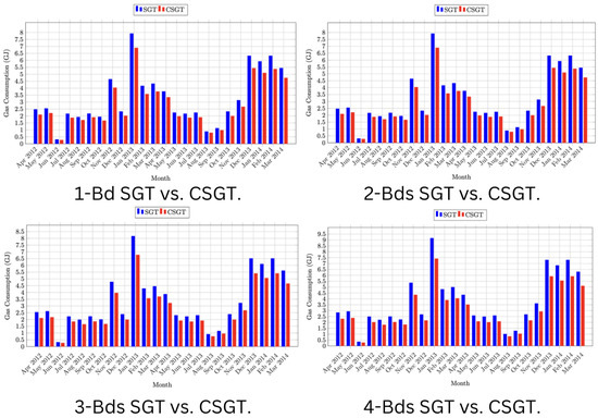
Figure 12.
Monthly gas consumption (2012–2014) for one to four bedroom SGTs and CSGTs in grid-connected mode.
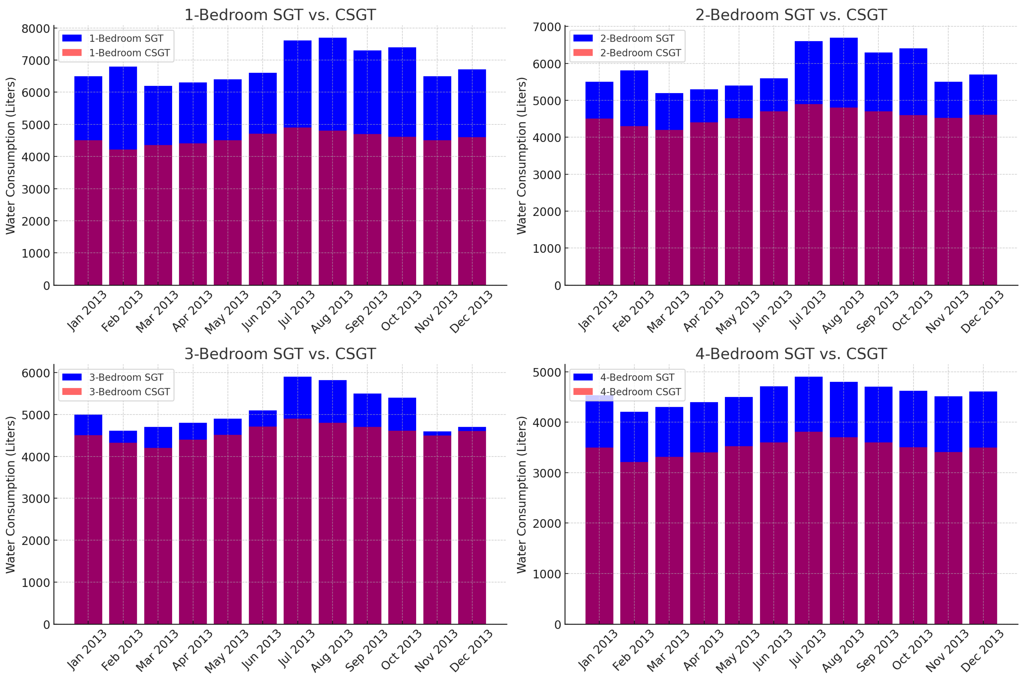
Figure 13 presents the total water consumption of one–four Bd SGTs and CSGTs in grid-connected mode for January–December 2013. This shows that CSGTs outperform SGTs in reducing water consumption for all unit sizes. In January 2013, the one-Bd CSGT used 4500 L, which is 30% less than the 6500 L for the one-Bd SGT. The shared infrastructure and smart water management systems contribute to these savings. For two-Bd units, the CSGT consumed 4500 L, which is 18% less than the 5500 L for the SGTs. For three- and four-Bd units, the CSGTs show reductions ranging from 10% to 23%.
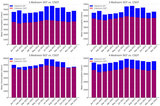
Figure 13.
Monthly total water consumption for one to four bedroom SGTs and CSGTs in grid-connected mode for January–December 2013.
Burnaby has a temperate oceanic climate with mild, wet winters and warm, dry summers. These conditions affect thermal comfort in SGTs. Indoor temperatures are usually kept above 18 C. Winter temperatures between 18 C and 20 C feel cool but comfortable, while the range of 20 C to 23 C is ideal for most of the year. In warmer months, indoor temperatures may reach 23 C to 25 C, which many find comfortable. However, on hot summer days, temperatures above 25 C can occur. Thus, effective cooling is essential to maintaining indoor comfort.
4.2. The Proposed ML Model Results
The proposed model was evaluated and compared with several well-known models, including LR, LSTM, CNN, RF, Gradient Boosting (GB), and hybrid LSTM-CNN. LR serves as a simple performance baseline. LSTM is good at handling sequential data, CNN is good at recognizing spatial patterns, RF is good at managing non-linear relationships and noisy data, GB improves accuracy through ensemble learning, and hybrid LSTM-CNN is good at capturing both temporal and spatial dependencies. These diverse approaches are considered to evaluate the effectiveness of the proposed model in optimizing energy performance [47].
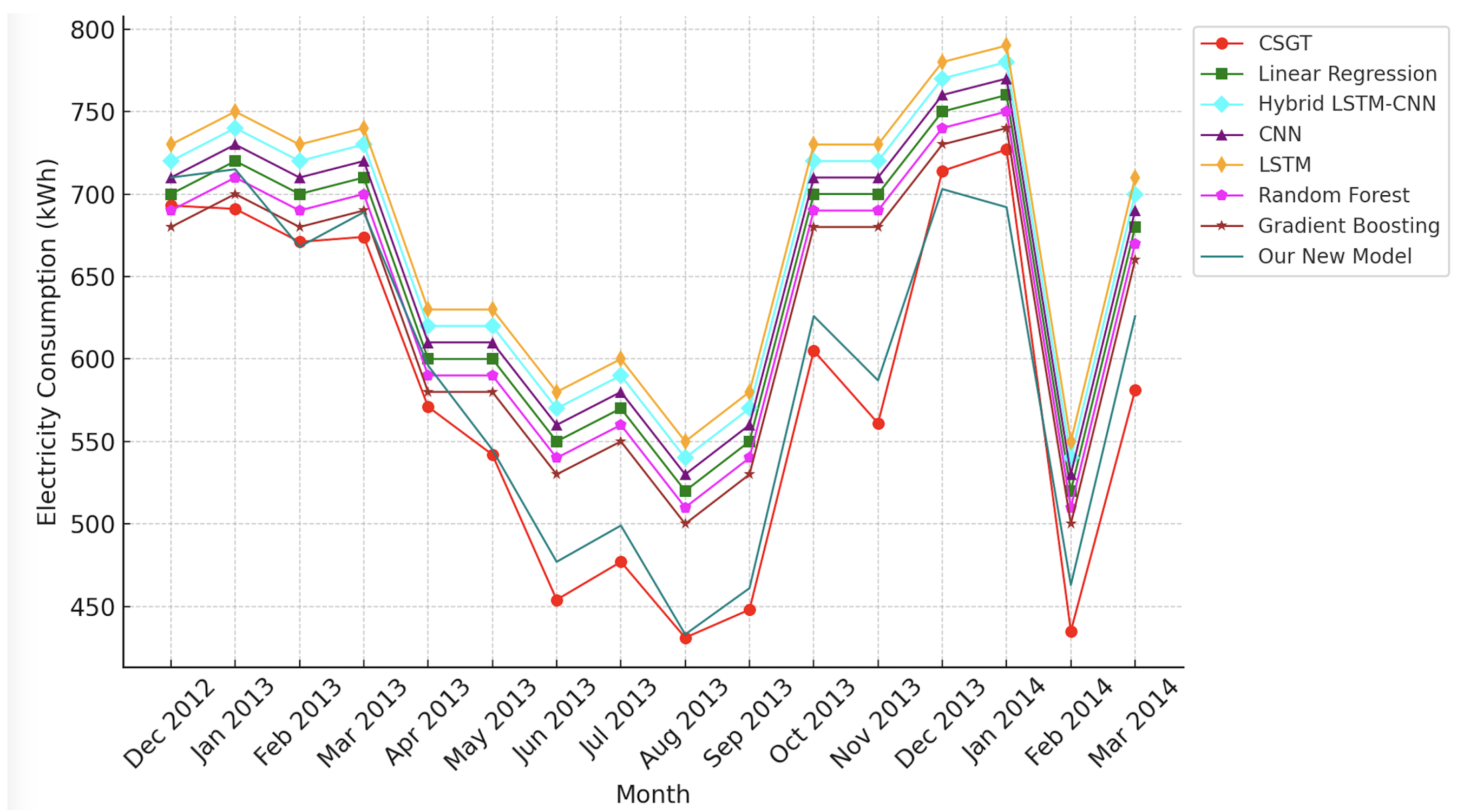
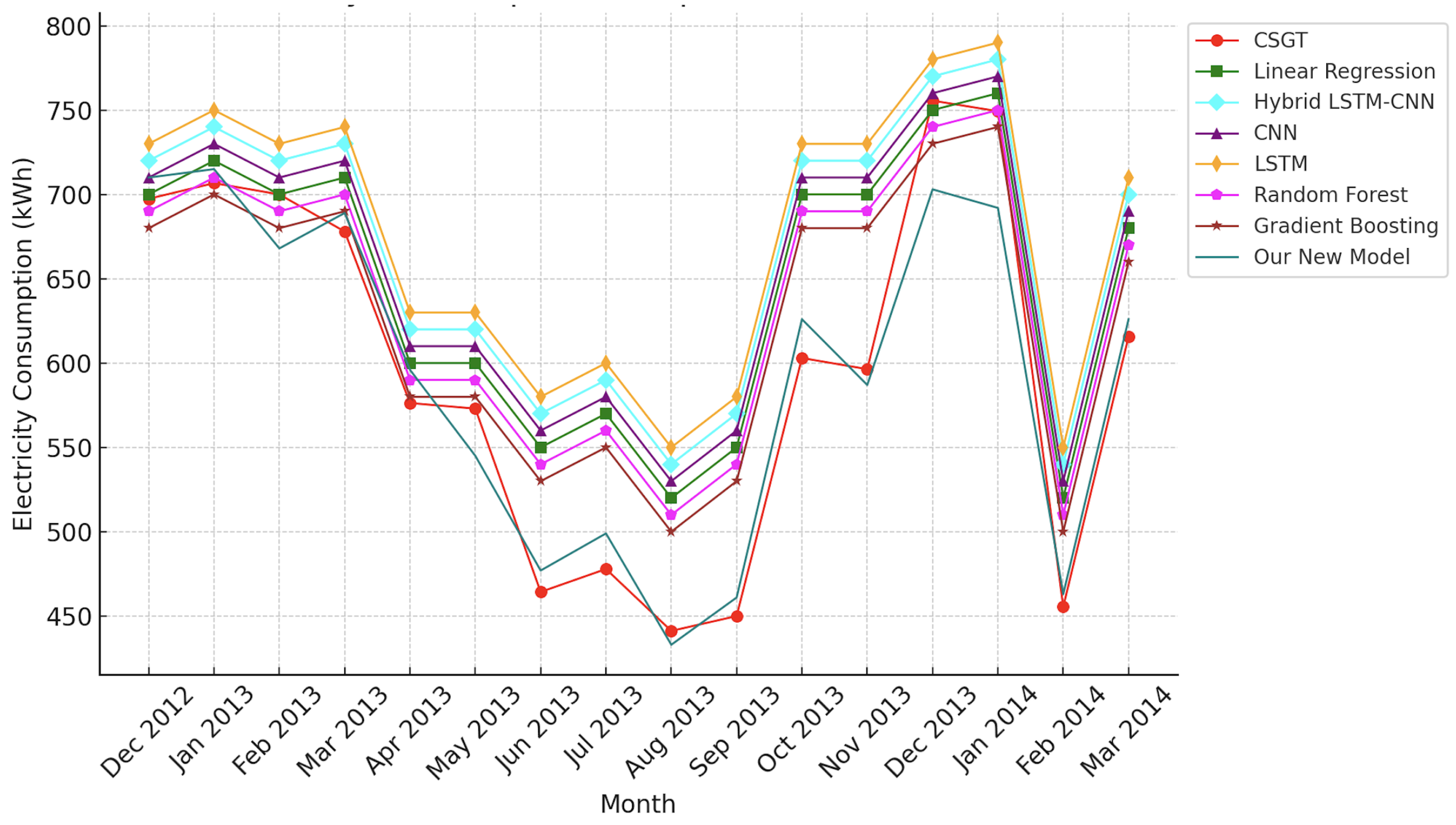
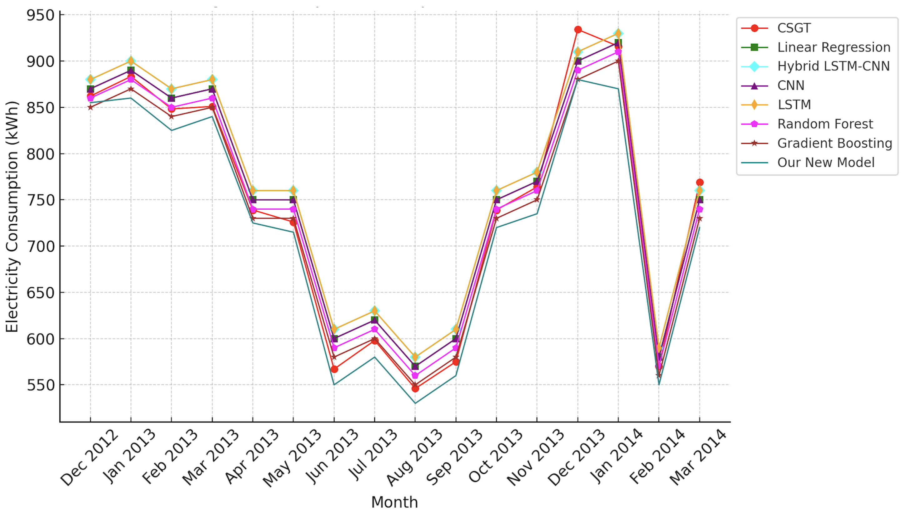
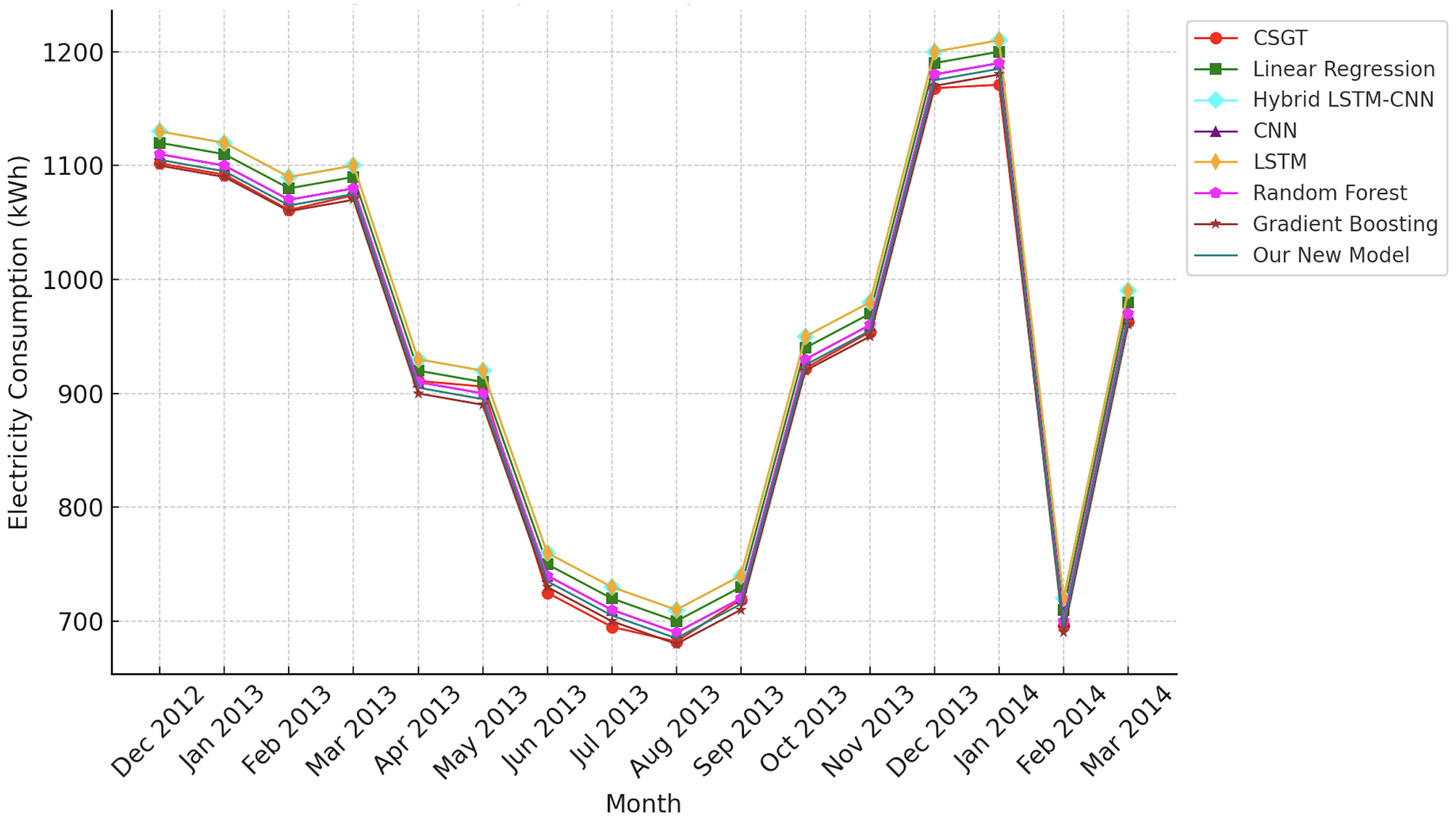
The monthly electricity consumption for one–four Bd CSGTs is given in Figure 14, Figure 15, Figure 16 and Figure 17, respectively. These show there are peaks in winter due to higher heating demands. As the number of bedrooms increases, so does electricity usage, with four-Bd units having the highest consumption. In addition, the proposed ML model outperforms the others with minimal deviation from the actual values. Thus, it adapts well to consumption patterns and provides precise estimates, even during low usage. The RMSE and for the proposed model indicate consistent predictions and superior performance compared with the other models.
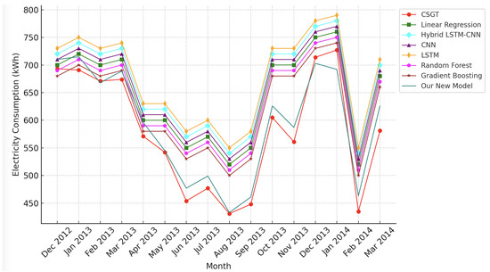
Figure 14.
Actual versus predicted monthly electricity consumption with seven ML models for a one bedroom CSGT in grid-connected mode for 2012–2014.
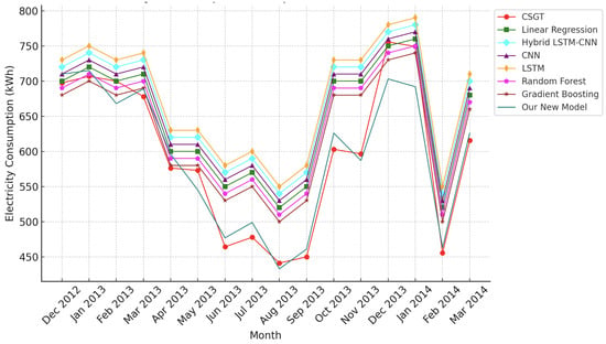
Figure 15.
Actual versus predicted monthly electricity consumption with seven ML models for a two bedroom CSGT in grid-connected mode (2012–2014).
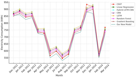
Figure 16.
Actual versus predicted monthly electricity consumption with seven ML models for a three bedroom CSGT in grid-connected mode (2012–2014).

Figure 17.
Actual versus predicted monthly electricity consumption with seven ML models for a four bedroom CSGT in grid-connected mode (2012–2014).
Table 7 presents the yearly performance for one–four Bd SGTs and CSGTs. These results highlight the benefits of CSGTs over SGTs, as there are improvements in resource efficiency, sustainability, and cost-effectiveness. CSGTs have better energy efficiency with heat loss of 5-8% compared with 7–10% for SGTs, indicating superior insulation and energy management. CSGTs maintain a tighter temperature range of ±1.5 C to ±3 C compared with ±3.5 C to ±5 C for SGTs, reflecting better HVAC control and indoor comfort. CSGTs have lower carbon emissions, from 0.18 kgCO2/kWh to 0.22 kgCO2/kWh, while SGTs range from 0.22 kgCO2/kWh to 0.26 kgCO2/kWh, indicating better use of RESs. CSGTs have lower HVAC operating costs, from 30 CAD/unit to 45 CAD/unit, compared with 40 CAD/unit to 55 CAD/unit for SGTs, so they are more efficient. Overall, CSGTs outperform SGTs in comfort, sustainability, and cost savings, making them a better choice for long-term savings and lower environmental impact.

Table 7.
Yearly performance for one to four bedroom SGTs and CSGTs.
Table 8 and Table 9 present the MAPE, RMSE, MAE, and for connected and disconnected SGTs with one to four bedrooms, with and without the proposed ML model. In Table 8, the MAPE is 3.51% (one-Bd) to 5.05% (four-Bd), RMSE is 2.79 kWh to 4.16 kWh, and MAE is 2.27 kWh to 3.62 kWh. The values range from 0.74 to 0.88, indicating good prediction. Table 9 shows the performance is improved with the proposed ML model. The MAPE decreases to 2.63% to 4.43%, RMSE drops to 1.93 kWh to 3.47 kWh, MAE decreases to 1.44 kWh to 3.06 kWh, and improves to 0.80 to 0.92. These results demonstrate that employing an ML model can significantly improve prediction performance and highlight the reliability and robustness of the proposed model in energy prediction for both SGTs and CSGTs. Table 8 and Table 9 also give the corresponding acceptable ranges. The terms “Very Good” and “Acceptable” represent thresholds for performance metrics. For one-Bd CSGTs (Figure 14), the range is 200 kWh, with a mean around 600–650 kWh. The two-Bd (Figure 15) and three-Bd (Figure 16) units have similar ranges with means of about 700 kWh. The four-Bd CSGT (Figure 17) has a range of 300 kWh and a mean of about 950 kWh. These values are within the acceptable range, confirming the reliability of the model.

Table 8.
Monthly energy performance of SGTs and CSGTs without an ML model.

Table 9.
Monthly energy performance of SGTs and CSGTs with an ML model.
Table 10 presents the parameters and performance of the 7 ML models, including the number of layers, neurons, training iterations per epoch, training time per epoch, error, and accuracy. These results show that the proposed model has the best performance with 95% accuracy and a low MAE of 0.015, but it has the highest computational cost due to its complex architecture. The hybrid LSTM-CNN model provides a good tradeoff between accuracy (90%) and efficiency, while GB (86%) and RF (85%) perform well with moderate training times and acceptable error rates. The LSTM and CNN models have comparable accuracy (82–83%) and error rates. LR has the lowest accuracy (78%) and highest MAE (0.05), which is expected since it is a simple baseline.

Table 10.
Number of layers, neurons, training iterations per epoch, training time per epoch, error, and accuracy for 7 ML models.
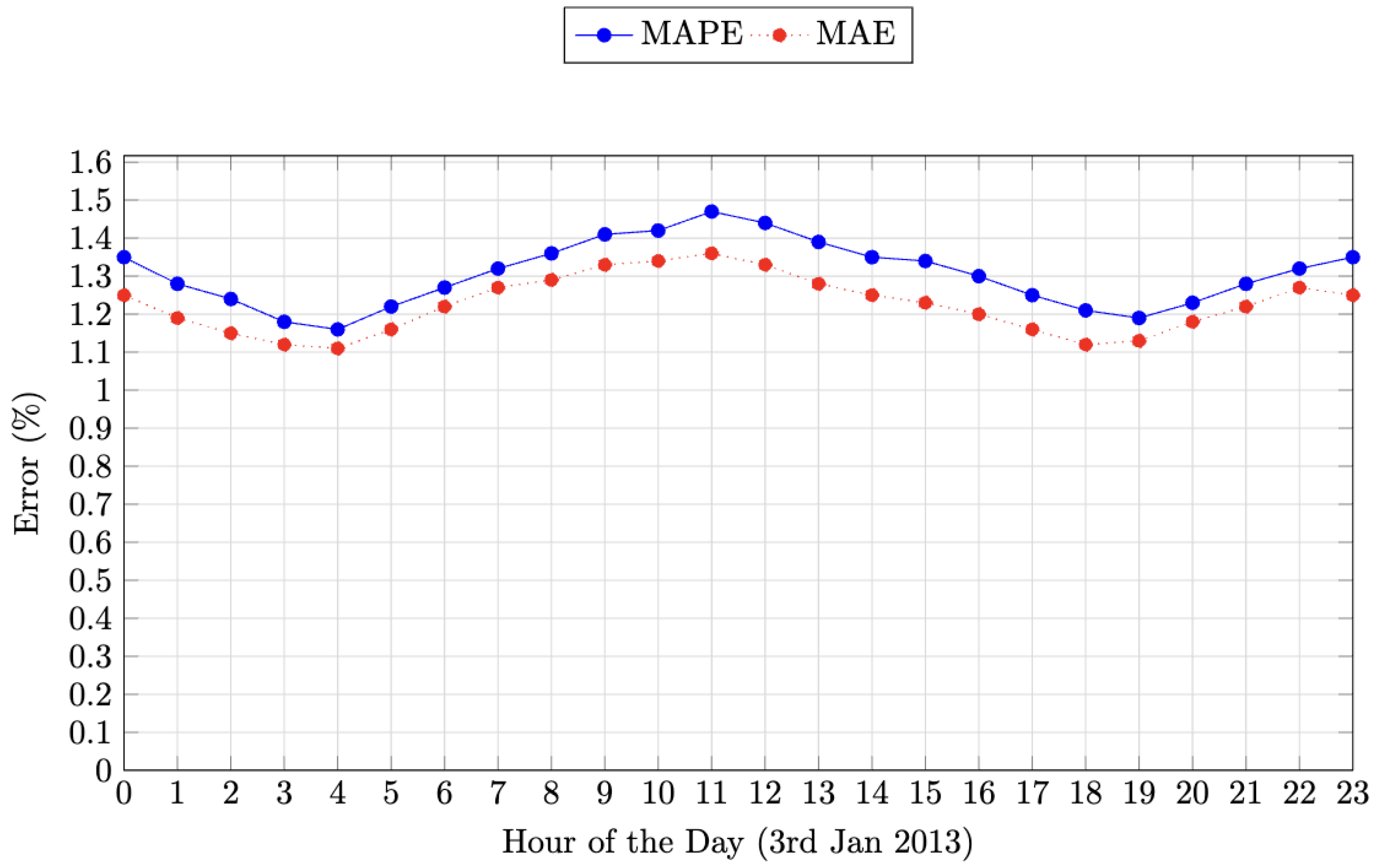
The MAPE and MAE for day-ahead predictions for CSGTs vary depending on weather, occupancy, and resource consumption behavior. Figure 18 gives the hourly variations in MAPE and MAE for day ahead predictions for 3 January 2013. This shows that the error fluctuations are between 1.2% and 1.6%, indicating consistent model performance throughout the day. Low MAPE and MAE suggest good accuracy, with minimal fluctuations confirming that the model can handle varying conditions and provide robust energy usage prediction.

Figure 18.
Hourly one day ahead prediction MAPE and MAE for 3 January 2013.
The normality and homoscedasticity residuals [75,76] are used to validate model performance. From January 3 to 10, 2013, the residuals (actual values - predicted values) ranged between 1 and −2 kWh, indicating good prediction accuracy. The normality (Shapiro–Wilk test) residual is and a value is normal if , so the normality is verified. The homoscedasticity (Breusch–Pagan test) residual is and indicates consistent variance. The lack of heteroscedasticity suggests that model predictions will be stable across a variety of data, indicating reliability and robustness. The normality and homoscedasticity confirm that the proposed model provides excellent energy prediction for grid-connected CSGTs. Note that practical challenges, including system integration, user acceptance, data privacy, and maintenance, should be considered for successful model deployment in real-world settings.
5. Conclusions
This paper presented a model for Connected Smart Green Townhouses (CSGTs) designed to optimize resource use. The integration of PV solar panels and efficient HVAC systems was shown to reduce resource consumption, promoting sustainable living. The results indicate improvements in cost, efficiency, performance, and accuracy for CSGTs in Burnaby, BC. The proposed deep hybrid ML model outperformed several well-known models, including Gradient Boosting (GB), Random Forest (RF), Long Short Term Memory (LSTM), Convolutional Neural Network (CNN), hybrid LSTM-CNN, and Linear Regression (LR).
The proposed model had lower Mean Absolute Percentage Error (MAPE), Root Mean Square Error (RMSE), and Mean Absolute Error (MAE), and higher , confirming its prediction precision. The accuracy ranged from 1.2% to 1.6%, with predictions closely aligning with actual values. Historical data, combined with model predictions, showed improvements in energy performance, cost savings, and emissions reduction. This indicates that the proposed model is effective for energy optimization in CSGTs. Future work will explore energy management policies and integrate more advanced models for improved system response and performance.
Author Contributions
Conception and design, S.M.M., T.A.G., I.T.C. and H.T.; preparation and analysis, S.M.M., I.T.C. and T.A.G.; writing—original draft, T.A.G., S.M.M. and I.T.C.; writing—review and editing, T.A.G., S.M.M., I.T.C. and H.T.; supervision, T.A.G. All authors have read and agreed to the published version of the manuscript.
Funding
This research received no external funding.
Data Availability Statement
The original contributions presented in the study are included in the article, further inquiries can be directed to the corresponding author.
Conflicts of Interest
The authors declare no conflicts of interest.
Abbreviations
The following abbreviations are used in this manuscript.
| Symbol | Description | Symbol | Description |
| ANN | Artificial Neural Network | LEED | Leadership in Energy and Environmental Design |
| BC | British Columbia | LED | Light Emitting Diode |
| BMS | Building Management System | LSTM | Long Short-Term Memory |
| CAD | Canadian Dollar | MAPE | Mean Absolute Percentage Error |
| CEI | Control Efficiency Index | MAE | Mean Absolute Error |
| CGBC | Canada Green Building Council | MG | Micro-Grid |
| CNN | Convolutional Neural Network | MRP | Material Recycling Percentage |
| COP | Coefficient of Performance | MSE | Mean Square Error |
| CSGT | Connected Smart Green Townhouse | NN | Neural Network |
| ECE | Electrical Consumption Efficiency | PV | Photovoltaic |
| EDA | Exploratory Data Analysis | REI | Renewable Energy Integration |
| EER | Energy Efficiency Ratio | RES | Renewable Energy Sources |
| GB | Green Building | SG | Smart Grid |
| GCE | Gas Consumption Efficiency | SGB | Smart Green Building |
| GHG | Greenhouse Gas | SGT | Smart Green Townhouse |
| GHGI | Greenhouse Gas Index | SOH | Size Of Home |
| HDD | Heating Degree Days | STLF | Short-Term Load Forecasting |
| HSPF | Heating Seasonal Performance Factor | STUI | Smart Technology Utilization Index |
| HVAC | Heating, Ventilation, and Air Conditioning | TEDI | Total Energy Demand Intensity |
| IAQ | Indoor Air Quality | TEUI | Total Energy Use Intensity |
| LR | Linear Regression | TWMU | Total Weight of Materials Used |
| ML | Machine Learning | VOC | Volatile Organic Compound |
| RF | Random Forest | WRM | Weight of Recycled Materials |
| RMSE | Root Mean Square Error | WRR | Waste Recycling Rate |
| SB | Smart Building | WRW | Weight of Recycled Waste |
| SEER | Seasonal Energy Efficiency Ratio |
References
- Omrany, H.; Soebarto, V.; Ghaffarianhoseini, A. Rethinking the concept of building energy rating system in Australia: A pathway to life-cycle net-zero energy building design. Archit. Sci. Rev. 2022, 65, 42–56. [Google Scholar] [CrossRef]
- Moran, P.; O’Connell, J.; Gotggins, J. Sustainable energy efficiency retrofits as residential buildings move towards nearly zero energy building (NZEB) standards. Energy Build. 2020, 211, 109816. [Google Scholar] [CrossRef]
- Ma, Z.; Zhao, D.; She, C.; Yang, Y.; Yang, R. Personal thermal management techniques for thermal comfort and building energy saving. Mater. Today Phys. 2021, 20, 100465. [Google Scholar] [CrossRef]
- Whitney, S.; Dreyer, B.C.; Riemer, M. Motivations, barriers and leverage points: Exploring pathways for energy consumption reduction in Canadian commercial office buildings. Energy Res. Soc. Sci. 2020, 70, 101687. [Google Scholar] [CrossRef]
- Vepsalainen, J.; Otto, K.; Lajunen, A.; Tammi, K. Computationally efficient model for energy demand prediction of electric city bus in varying operating conditions. Energy 2019, 169, 433–443. [Google Scholar] [CrossRef]
- Hasanova, N.; Neşe, S.V. Demand-side energy management in smart buildings: A case study. Eur. J. Tech. 2021, 11, 239–247. [Google Scholar] [CrossRef]
- Habiba, U.; Ahmed, I.; Asif, M.; Alhelou, H.H.; Khalid, M. A review on enhancing energy efficiency and adaptability through system integration for smart buildings. J. Build. Eng. 2024, 89, 109354. [Google Scholar] [CrossRef]
- Dagdougui, H.; Bagheri, F.; Le, H.; Dessaint, L. Neural network model for short-term and very-short-term load forecasting in district buildings. Energy Build. 2019, 203, 109408. [Google Scholar] [CrossRef]
- Godinho, X.; Bernardo, H.; Oliveira, F.T.; Sousa, J.C. Forecasting heating and cooling energy demand in an office building using machine learning methods. In Proceedings of the International Young Engineers Forum, Costa da Caparica, Portugal, 3 July 2020; pp. 1–6. [Google Scholar]
- Edalatnia, S.; Das, R.R. Building benchmarking and energy performance: Analysis of social and affordable housing in British Columbia, Canada. Energy Build. 2024, 313, 114259. [Google Scholar] [CrossRef]
- Akkiraju, R.; Sinha, V.; Xu, A.; Mahmud, J.; Gundecha, P.; Liu, Z.; Liu, X.; Schumacher, J. Characterizing machine learning processes: A maturity framework. In Proceedings of the Business Process Management: 18th International Conference, BPM 2020, Seville, Spain, 13–18 September 2020; pp. 17–31. [Google Scholar] [CrossRef]
- Welte, R.; Estler, M.; Lucke, D. A method for implementation of machine learning solutions for predictive maintenance in small and medium sized enterprises. Procedia CIRP 2020, 93, 909–914. [Google Scholar] [CrossRef]
- Sultana, J.; Singha, A.K.; Siddiqui, S.T.; Nagalaxmi, G.; Sriram, A.K.; Pathak, N. COVID-19 Pandemic Prediction and Forecasting Using Machine Learning Classifiers. Intell. Autom. Soft Comput. 2022, 32, 1007–1024. [Google Scholar] [CrossRef]
- Aneeque, A.M.; Alghassab, M.; Ullah, K.; Khan, Z.A.; Lu, Y.; Imran, M. A review of electricity demand forecasting in low and middle income countries: The demand determinants and horizons. Sustainability 2020, 12, 5931. [Google Scholar] [CrossRef]
- EIA. Monthly Energy Review—June 2020; U.S. Energy Information Administration: Washington, DC, USA, 2020. Available online: https://www.eia.gov/totalenergy/data/monthly/archive/00352006.pdf (accessed on 8 May 2024).
- Kelly, S.; Crawford-Brown, D.; Pollitt, M.G. Building performance evaluation and certification in the UK: Is SAP fit for purpose? Renew. Sustain. Energy Rev. 2012, 16, 6861–6878. [Google Scholar] [CrossRef]
- Runge, J.; Zmeureanu, R. Forecasting energy use in buildings using artificial neural networks: A review. Energies 2019, 12, 3254. [Google Scholar] [CrossRef]
- Li, Y.L.; Han, M.Y.; Liu, S.Y.; Chen, G.Q. Energy consumption and greenhouse gas emissions by buildings: A multi-scale perspective. Build. Environ. 2019, 150, 240–250. [Google Scholar] [CrossRef]
- Li, Y.; Wang, W.; Wang, Y.; Xin, Y.; He, T.; Zhao, G. A review of studies involving the effects of climate change on energy consumption for building heating and cooling. Int. J. Environ. Res. Public Health 2021, 18, 40. [Google Scholar] [CrossRef]
- Talib, R.; Nabil, N.; Choi, W. Optimization-based data-enabled modeling technique for HVAC systems components. Buildings 2020, 10, 163. [Google Scholar] [CrossRef]
- Homod, R.Z. Analysis and optimization of HVAC control systems based on energy and performance considerations for smart buildings. Renew. Energy 2018, 126, 49–64. [Google Scholar] [CrossRef]
- Condon, F.; Martínez, J.M.; Eltamaly, A.M.; Kim, Y.C.; Ahmed, M.A. Design and implementation of a cloud-IoT-based home energy management system. Sensors 2022, 23, 176. [Google Scholar] [CrossRef]
- Moghimi, S.M.; Shariatmadar, S.M.; Dashti, R. Active-reactive power stability analysis in a micro grid in grid-connected mode based on particle swarm optimization (PSO) including model information. Phys. Sci. Int. J. 2016, 10, 1–12. [Google Scholar] [CrossRef]
- Rafiee Sandgani, M. Coordinated Energy Management in a Network of Microgrids. Ph.D. Thesis, McMaster University, Hamilton, ON, Canada, 2018. Available online: http://hdl.handle.net/11375/23043 (accessed on 8 May 2024).
- Makonin, S. Electricity, water, and natural gas consumption of a residential house in Canada from 2012 to 2014. Sci. Data 2016, 3, 160037. [Google Scholar] [CrossRef]
- Bahmanyar, D.; Razmjooy, N.; Mirjalili, S. Multi-objective scheduling of IoT-enabled smart homes for energy management based on arithmetic optimization algorithm: A node-RED and nodeMCU module-based technique. Knowl.-Based Syst. 2022, 247, 108762. [Google Scholar] [CrossRef]
- Zhou, X.; Du, H.; Xue, S.; Ma, Z. Recent advances in data mining and machine learning for enhanced building energy management. Sustain. Cities Soc. 2024, 66, 132636. [Google Scholar] [CrossRef]
- Berardi, U.; Jafarpur, P. Assessing the impact of climate change on building heating and cooling energy demand in Canada. Renew. Sustain. Energy Rev. 2020, 121, 109681. [Google Scholar] [CrossRef]
- Makonin, S.; Popowich, F.; Bartram, L.; Gill, B.; Bajić, I.V. AMPds: A public dataset for load disaggregation and eco-feedback research. In Proceedings of the 2013 IEEE Electrical Power & Energy Conference, Halifax, NS, Canada, 21–23 August 2013. [Google Scholar] [CrossRef]
- Gaur, M.; Makonin, S.; Bajić, I.V.; Majumdar, A. Performance evaluation of techniques for identifying abnormal energy consumption in buildings. IEEE Access 2019, 7, 62721–62733. [Google Scholar] [CrossRef]
- Lin, B.; Chen, Z. Net zero energy building evaluation, validation and reflection—A successful project application. Energy Build. 2022, 261, 111946. [Google Scholar] [CrossRef]
- Adier, M.F.V.; Sevilla, M.E.P.; Valerio, D.N.R.; Ongpeng, J.M.C. Bamboo as Sustainable Building Materials: A Systematic Review of Properties, Treatment Methods, and Standards. Buildings 2023, 13, 2449. [Google Scholar] [CrossRef]
- Susanto, D.; Widyarko, W. Sustainable Material: Used Wood As Building Material. INSIST 2017, 2, 14–18. [Google Scholar] [CrossRef][Green Version]
- Yu, B.; Fingrut, A. Sustainable building design (SBD) with reclaimed wood library constructed in collaboration with 3D scanning technology in the UK. Resour. Conserv. Recycl. 2022, 179, 106566. [Google Scholar] [CrossRef]
- Bribián, I.Z.; Capilla, A.V.; Uson, A.A. Life cycle assessment of building materials: Comparative analysis of energy and environmental impacts and evaluation of the eco-efficiency improvement potential. Build. Environ. 2011, 46, 1133–1140. [Google Scholar] [CrossRef]
- Stoikov, V.; Gassiy, V. Energy efficiency of housing as a tool for sustainable development. MATEC Web Conf. 2018, 251, 03061. [Google Scholar] [CrossRef]
- Gado, A.; Ibrahim, M.; Youssef, A. Feasibility of rainwater harvesting for sustainable water management in urban areas of Egypt. Environ. Sci. Pollut. Res. 2020, 27, 32304–32317. [Google Scholar] [CrossRef] [PubMed]
- Decuypere, R.; Robaeyst, B.; Hudders, L.; Baccarne, B.; Van de Sompel, D. Transitioning to energy efficient housing: Drivers and barriers of intermediaries in heat pump technology. Energy Policy 2021, 156, 112709. [Google Scholar] [CrossRef]
- Benavente-Peces, C. On the energy efficiency in the next generation of smart buildings—Supporting technologies and techniques. Energies 2019, 12, 4399. [Google Scholar] [CrossRef]
- Maasoumy, M.; Sangiovanni-Vincentelli, A. Smart connected buildings design automation: Foundations and trends. Found. Trends Electron. Des. Autom. 2016, 12, 1–143. [Google Scholar] [CrossRef]
- Vosoughkhosravi, S.; Dixon-Grasso, L.; Jafari, A. The impact of LEED certification on energy performance and occupant satisfaction: A case study of residential college buildings. J. Build. Eng. 2022, 59, 105097. [Google Scholar] [CrossRef]
- Thomas, D.; Deblecker, O.; Ioakimidis, C.S. Optimal operation of an energy management system for a grid-connected smart building considering photovoltaics’ uncertainty and stochastic electric vehicles’ driving schedule. Appl. Energy 2018, 210, 1188–1206. [Google Scholar] [CrossRef]
- Moghimi, S.M.; Shariatmadar, S.M.; Dashti, R. Stability analysis of the micro-grid operation in micro-grid mode based on particle swarm optimization (PSO) including model information. Phys. Sci. Int. J. 2016, 10, 1–13. [Google Scholar] [CrossRef]
- Amir, V.; Jadid, S.; Ehsan, M. Operation of networked multi-carrier microgrid considering demand response. Compel. Int. J. Comput. Math. Electr. Electron. Eng. 2019, 38, 724–744. [Google Scholar] [CrossRef]
- Jangsten, M.; Lindholm, T.; Dalenbäck, J.O. Analysis of operational data from a district cooling system and its connected buildings. Energy 2020, 203, 117844. [Google Scholar] [CrossRef]
- Agugiaro, G.; Zwamborn, A.; Tigchelaar, C.; Matthijssen, E.; León-Sánchez, C.; van der Molen, F.; Stoter, J. On the influence of party walls for urban energy modelling. Int. Arch. Photogramm. Remote Sens. Spatial Inf. Sci. 2022, 48, 9–16. [Google Scholar] [CrossRef]
- Palmer, J.; Terry, N. Looking critically at heat loss through party walls. Sustainability 2022, 14, 3072. [Google Scholar] [CrossRef]
- Kim, D.; Yoon, Y.; Lee, J.; Mago, P.J.; Lee, K.; Cho, H. Design and implementation of smart buildings: A review of current research trends. Energies 2022, 15, 4278. [Google Scholar] [CrossRef]
- Mariano-Hernández, D.; Hernández-Callejo, L.; García, F.S.; Duque-Perez, O.; Zorita-Lamadrid, A.L. A review of energy consumption forecasting in smart buildings: Methods, input variables, forecasting horizon and metrics. Appl. Sci. 2020, 10, 8323. [Google Scholar] [CrossRef]
- Raschka, S.; Patterson, J.; Nolet, C. Machine learning in Python: Main developments and technology trends in data science, machine learning, and artificial intelligence. Information 2020, 11, 193. [Google Scholar] [CrossRef]
- Harris, C.R.; Millman, K.J.; Van der Walt, S.J.; Gommers, R.; Virtanen, P.; Cournapeau, D.; Wieser, E.; Taylor, J.; Berg, S.; Smith, N.J.; et al. Array programming with NumPy. Nature 2020, 585, 357–362. [Google Scholar] [CrossRef] [PubMed]
- Hunter, J.D. Matplotlib: A 2D graphics environment. Comput. Sci. Eng. 2007, 9, 90–95. [Google Scholar] [CrossRef]
- Pfenninger, S.; Staffell, I. Long-term patterns of European PV output using 30 years of validated hourly reanalysis and satellite data. Energy 2016, 114, 1251–1265. [Google Scholar] [CrossRef]
- Sharma, R.; Goel, S. Performance analysis of a 11.2 kWp roof top grid-connected PV system in Eastern India. Energy Rep. 2017, 3, 103–112. [Google Scholar] [CrossRef]
- Duffie, J.A.; Beckman, W.A.; Blair, N. Solar Engineering of Thermal Processes, Photovoltaics and Wind; John Wiley & Sons: Hoboken, NJ, USA, 2020. [Google Scholar] [CrossRef]
- Lin, C.; Gao, Y.; Huang, J.; Shi, D.; Feng, W.; Liu, Q.; Du, X. A novel numerical model for investigating macro factors influencing building energy consumption intensity. Sustain. Prod. Consum. 2020, 24, 205–218. [Google Scholar] [CrossRef]
- Goetzler, W.; Guernsey, M.; Young, J.; Fujrman, J.; Abdelaziz, A. The Future of Air Conditioning for Buildings (DOE/EE-1394); Navigant Consulting: Burlington, MA, USA, 2016. [Google Scholar] [CrossRef]
- Henderson, J. An Investigation into the Resilience and Durability of High R-Value Exterior Insulated Wood Framed Walls in Cold Climates Assessed Using In-situ Measurement and Calibrated Hygrothermal Modeling. Master’s Thesis, Toronto Metropolitan University, Toronto, ON, USA, 2021. [Google Scholar] [CrossRef]
- Lawton, M.; Roppel, P.; Fookes, D.; Teasdale, A.; Schoonhoven, D. Real R-Value of Exterior Insulated Wall Assemblies. BEST2 Conf.: Building Enclosure Science and Technology. National Institute of Building Sciences. 2010. Available online: https://api.semanticscholar.org/CorpusID:135465676 (accessed on 8 May 2024).
- Chan, J.; Frisque, A.; Jang, A. Designing to TEDI, TEUI, and GHGI performance metrics. In Proceedings of the International Building Performance Simulation Association Conference, Rome, Italy, 2–4 September 2019; pp. 4053–4060. [Google Scholar] [CrossRef]
- Saxena, H.; Aponte, O.; McConky, K.T. A hybrid machine learning model for forecasting a billing period’s peak electric load days. Int. J. Forecast. 2019, 35, 1288–1303. [Google Scholar] [CrossRef]
- Lu, C.; Li, S.; Gu, J.; Lu, W.; Olofsson, T.; Ma, J. A hybrid ensemble learning framework for zero-energy potential prediction of photovoltaic direct-driven air conditioners. J. Build. Eng. 2023, 64, 105602. [Google Scholar] [CrossRef]
- Moghimi, S.M.; Gulliver, T.A.; Chelvan, I.T. Energy management in modern buildings based on demand prediction and machine learning—A review. Energies 2024, 17, 555. [Google Scholar] [CrossRef]
- Khan, Z.A.; Hussain, T.; Ullah, A.; Rho, S.; Lee, M.; Baik, S.W. Towards efficient electricity forecasting in residential and commercial buildings: A novel hybrid CNN with a LSTM-AE based framework. Sensors 2020, 20, 1399. [Google Scholar] [CrossRef]
- Elmaz, F.; Eyckerman, R.; Casteels, W.; Latré, S.; Hellinckx, P. CNN-LSTM architecture for predictive indoor temperature modeling. Build. Environ. 2021, 206, 108327. [Google Scholar] [CrossRef]
- Vartanian, C.; Paiss, M.; Viswanathan, V.; Kolln, J.T.; Reed, D.M. Review of codes and standards for energy storage systems. Curr. Sustain. Renew. Energy Rep. 2021, 8, 138–148. [Google Scholar] [CrossRef]
- Ashenov, N.; Myrzaliyeva, M.; Mussakhanova, M.; Nunna, H.K. Dynamic cloud and ANN based home energy management system for end-users with smart-plugs and PV generation. In Proceedings of the IEEE Texas Power and Energy Conference, Online, 2–5 February 2021. [Google Scholar] [CrossRef]
- Arora, S.; Taylor, J.W. Short-term forecasting of anomalous load using rule-based triple seasonal methods. IEEE Trans. Power Syst. 2013, 28, 3235–3242. [Google Scholar] [CrossRef]
- Huang, N.; Lu, G.; Xu, D. A permutation importance-based feature selection method for short-term electricity load forecasting using random forest. Energies 2016, 9, 767. [Google Scholar] [CrossRef]
- Syed, D.; Abu-Rub, H.; Ghrayeb, A.; Refaat, S.S.; Houchati, M.; Bouhali, O.; Bañales, S. Deep learning-based short-term load forecasting approach in smart grid with clustering and consumption pattern recognition. IEEE Access 2021, 9, 54992–55008. [Google Scholar] [CrossRef]
- Sendra-Arranz, R.; Gutiérrez, A. A long short-term memory artificial neural network to predict daily HVAC consumption in buildings. Energy Build. 2020, 216, 109952. [Google Scholar] [CrossRef]
- Luque, J.; Personal, E.; Garcia-Delgado, A.; Leon, C. Monthly electricity demand patterns and their relationship with the economic sector and geographic location. IEEE Access 2021, 9, 86254–86267. [Google Scholar] [CrossRef]
- Vaswani, A.; Shazeer, N.; Parmar, N.; Uszkoreit, J.; Jones, L.; Gomez, A.N.; Kaiser, Ł.; Polosukhin, I. Attention Is All You Need. Adv. Neural Inf. Process. Syst. 2017, 30. Available online: https://proceedings.neurips.cc/paper/2017/file/3f5ee243547dee91fbd053c1c4a845aa-Paper.pdf (accessed on 8 May 2024).
- Farsi, Z.; Walde, M.; Klementowicz, A.E.; Paraskevopoulou, F.; Woehler, A. Single synapse glutamate imaging reveals multiple levels of release mode regulation in mammalian synapses. iScience 2021, 24, 101933. [Google Scholar] [CrossRef] [PubMed]
- Jochmans, K. Heteroscedasticity-Robust inference in linear regression models with many covariates. J. Am. Stat. Assoc. 2022, 117, 887–896. [Google Scholar] [CrossRef]
- Mishra, P.; Pandey, C.M.; Singh, U.; Gupta, A.; Sahu, C.; Keshri, A. Descriptive statistics and normality tests for statistical data. Ann. Card. Anaesth. 2019, 22, 67–72. [Google Scholar] [CrossRef]
Disclaimer/Publisher’s Note: The statements, opinions and data contained in all publications are solely those of the individual author(s) and contributor(s) and not of MDPI and/or the editor(s). MDPI and/or the editor(s) disclaim responsibility for any injury to people or property resulting from any ideas, methods, instructions or products referred to in the content. |
© 2024 by the authors. Licensee MDPI, Basel, Switzerland. This article is an open access article distributed under the terms and conditions of the Creative Commons Attribution (CC BY) license (https://creativecommons.org/licenses/by/4.0/).

