Abstract
To improve the control performance and energy efficiency of the hydrostatic transmission (HST) system of wheel loaders, this study proposes a novel variable structure dual-motor hydrostatic transmission system, accompanied by a multivariable control strategy based on fuzzy sliding mode control. By constructing a simulation model of the transmission system, the performance of the novel transmission system is verified, and the control effects of common control strategies are compared. The simulation results show that the proposed control strategy and system have good matching and can adapt to disturbances actively. Field experiment results show that the proposed solution can achieve smooth automatic shifting of wheel loaders, while effectively adjusting system pressure, flow, and power. Compared with the traditional hydrodynamic torque converter loader transmission system, its transmission efficiency is effectively increased by 30%, and the efficiency is increased by 8% compared with the traditional hydrostatic transmission system This achievement is of great significance for improving the working efficiency of wheel loaders and reducing energy consumption. The future research focus is to further improve the multivariable control strategy, achieve intelligent operation, and improve the efficiency and reliability of the transmission system.
1. Introduction
Wheel loaders are considered one of the most widely used construction equipment machinery, extensively used in infrastructure construction [1]. To accommodate various loads, loaders generally use hydraulic mechanical drive methods, such as traditional automatic transmissions. The hydrodynamic torque converter is a key power transmission mechanism, playing the role of an energy converter in hydraulic drive [2].
However, the hydrodynamic torque converter has been proven to have high power loss during transmission, leading to problems such as low transmission efficiency and poor fuel economy [3,4]. To further improve the fuel efficiency of wheel loaders, hydrostatic transmission technology has been proposed to replace the traditional hydrodynamic torque converter system [5]. The current optimization direction is achieved through the series combination of multiple pumps or motors, replacing the traditional mechanical step speed regulation method with volume speed regulation. For example, Wang and Chen [6] designed a single fixed-pump single-variable motor hydrostatic system, replacing the large displacement variable motor by encoding multiple fixed small displacement motors. Han and Su [7] designed a dual pump confluence system, where two fixed pumps simultaneously supply oil to a variable motor, avoiding unnecessary overflow. Comellas and Pijuan [8] designed an off-road vehicle HST system with multiple drive axles. The system design has two identical hydraulic drive systems driving the front and rear parts of the off-road vehicle separately, eliminating the complicated gear group transmission.
The working environment of the loader is generally complex, needing to cope with various road conditions. This requires the loader’s transmission system to make timely adjustments according to different situations, but there is currently no transmission system structure that can change as needed. In response to this problem, a new Variable Structure Dual-Motor Hydrostatic Transmission system (VSM-HST) is designed. This system uses a dual-motor parallel drive, and the volume of the pump and motor can be adjusted, which increases the efficient adjustment range and speed width of the loader. At the same time, the change from single-motor drive to dual-motor drive mode is achieved by controlling the clutch. Because the displacement of the motor used is different, the change in the drive mechanism can meet the different speed and torque requirements of the loader under different road conditions.
As a hydraulic system, the HST system has typical nonlinear control characteristics. In engineering practice, methods of local linear control or control strategies with large fault tolerance are often used, such as Proportional Integral Control (PID), adaptive control, and sliding mode control. Saber [9] proposed a recursive identification model for a single-variable pump-fixed motor HST system, introducing the parameter changes in pump displacement and motor torque into the system by locally linearizing the hydraulic system. Joni and Reza [10] designed a loader drive system with a single-variable pump and multiple-variable motors and also designed a Proportional Integral Controller (PID) with state feedback, ensuring the smoothness of speed regulation. Hoang and Hyung [11] designed a two-stage control hydrostatic energy-saving system (SC-HST), using a single-variable pump to drive a single-variable motor design and proposed an adaptive sliding mode control strategy to solve the nonlinear characteristics of system control and external disturbance problems. Through experimental comparison, it was proven that its control performance is significantly better than PID control. Horst and Eckhard [12] proposed a hydrostatic transmission wind turbine actuator fault diagnosis and fault-tolerant control, using a Takagi–Sugeno sliding mode observer for fault compensation, correcting the control input by detecting the control parameter difference between the actual actuator and the virtual actuator. The simulation experiment proved that it has better control performance and fault tolerance mechanism than traditional PID control and adaptive control.
Because the designed transmission system needs to control the displacement of the pump and two motors at the same time and the structure of the system also needs to change with demand, using sliding mode control alone requires a lot of time and effort in the debugging process. Therefore, Fuzzy Sliding Mode Control (FSMC) is used. By formulating appropriate fuzzy rules, the control strategy can self-adjust with the change in the system structure, enhancing the anti-interference ability. In order to better match the control strategy with the system, adaptive improvements are made, and a Fuzzy Sliding Mode Control strategy based on multivariable control (MCF–SMC) is proposed, which is only for the VSM-HST system control. The simulation experiment proves that compared with traditional control, this strategy has better control characteristics for the VSM-HST system.
The novel Variable Structure Dual-Motor Hydrostatic Transmission system for loaders proposed in this paper has the characteristics of a variable structure, smooth speed regulation, and wide speed regulation range, which can meet the speed requirements of loaders for different road conditions. Compared with existing research, the main contributions of this paper are as follows:
- (a)
- A new hydrostatic transmission VSM-HST system is proposed, and its working principle, structural layout, and system characteristics are analyzed.
- (b)
- The speed and power requirements for the V-type operation of the VSM-HST loader system are discussed. The corresponding design parameters of the system are then determined.
- (c)
- The state equations of the VSM-HST system are developed, and a control strategy using MCF–SMC suitable for the system is formulated and evaluated. Simulation experiments are performed to compare the performance with several state-of-the-art strategies.
- (d)
- Together with the loader manufacturer, the initial prototype of a 7-ton loader, which features the VSM-HST system and its corresponding control strategy, was developed and successfully applied in actual engineering product production.
This paper is composed of five sections. Section 2 details the operational principle, function, operating environment, and fundamental parameter settings of the VSM-HST system and establishes a simulated experimental model. Section 3 outlines the mathematical model of MCF–SMC control, including the control principle and the impact of simulated control. Section 4 details the procedures, techniques, and results of the experiments while assessing the effectiveness of the system and control methods through comparative analysis. In addition, Section 5 outlines the main conclusions of the study.
2. System Analysis
Distinguished from conventional hydrostatic transmission systems that employ mechanical or hydraulic control methods, the novel system utilizes an integrated pump and motor configuration with an electro-hydraulic proportional control (EP) mode [13].
2.1. Working Principle
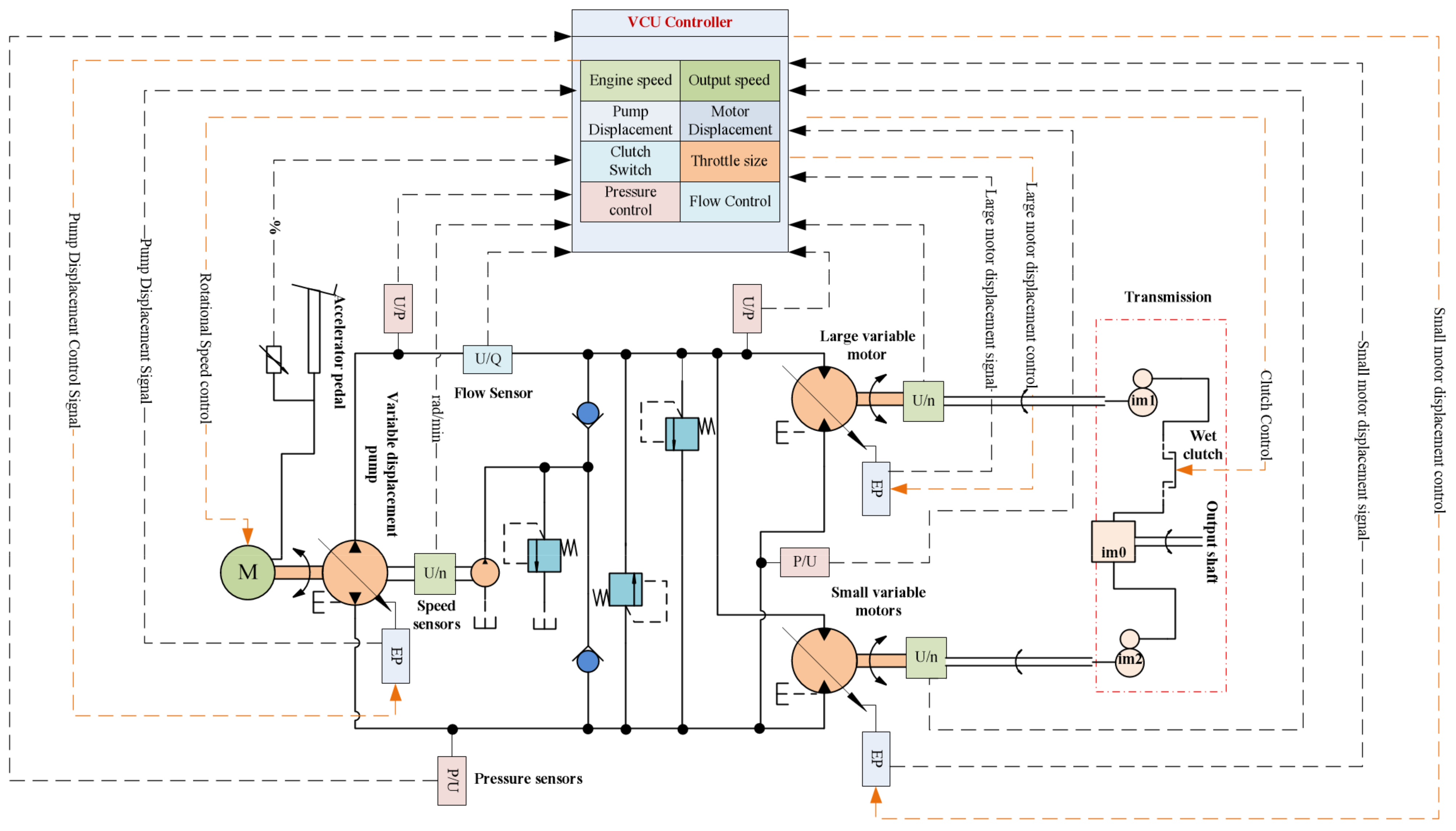
In Figure 1, the VSM-HST system exhibits a distinct configuration. The engine interfaces directly with the variable pump, channeling power into the hydraulic circuit to convert mechanical energy into hydraulic energy. The high-displacement variable motor (M1) and the low-displacement variable motor (M2) convert hydraulic energy into kinetic energy through the pressure differential at the inlet and outlet ports. These two motors are connected to the transmission and transmit power to the drive axle via gear sets within the transmission. The transmission between M1 and the output shaft is controlled by a clutch. The clutch can be disengaged to improve mechanical efficiency when M1 displacement is minimal. The displacement of the pump and motor is controlled by the EP control method, and the size of the displacement is directly controlled by the size of the input current. Changes in the equivalent total displacement of the system lead to variations in pressure, flow rate, output speed, and torque. Control of various parameters can be achieved by adjusting engine speed, pump, and motor displacement. The vehicle communication relies on Controller Area Network bus technology (CAN2.0B), which transforms system state data, including pressure, flow rate, pump and motor displacement, engine speed, throttle position, and output speed into messages sent to the Vehicle Control Unit (VCU). The VCU processes these data according to predetermined procedures and control strategies, transmitting computed results back as messages to respective actuators to execute system control. Its features perform the following:
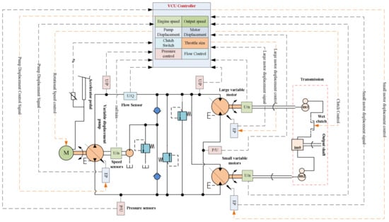
Figure 1.
VSM-HST system working principle.
- (1)
- Realize automatic gear shifting throughout the entire V-shape operating scenario.
- (2)
- Realize integrated control of multiple variables in the system to match input power with output power, thereby reducing overflow losses and engine idling and improving total system efficiency.
- (3)
- Effectively track the target vehicle speed and reduce the impact of load changes on the vehicle speed.
The following section elaborates in detail on the performance of the system from three aspects: speed characteristics, control characteristics, and torque characteristics and presents mathematical expressions and relationships concerning the speed, control, and torque characteristics of the system.
2.2. System Features
Speed Characteristics: Within the VSM-HST circuit, both pump and motor displacements are variable, and the relationship between motor speed and pump displacement adjustment parameters defines the speed characteristics. Without considering pipeline leakage, the output flow rate of the variable pump equals the sum of the input flow rates of the two parallel motors. This can be deduced from the continuity equation of flow, as Equation (1) shows:
where rotational speed, actual displacement, and volumetric efficiency of the pump are denoted as , and , respectively, while the rotational speed, actual displacement, and volumetric efficiency of M1 are denoted as , and , respectively, and the rotational speed, actual flow rate, and volumetric efficiency of M2 are denoted as , , and , respectively.
Synchronizing the two variable motors by engaging the gears in the gearbox, the speed relationship is as follows:
where and represent the values of the speed ratios of the M1 and M2 interconnected gear sets.
Associative Equations (1) and (2) provide expressions for the speeds of M1 and M2 as Equation (3) and Equation (4), respectively.
Control Characteristics: An analysis of the differing speed requirements for various operating conditions of the wheel loader (elaborated in Section 2.3) reveals the control characteristics as the relationship between changes in pump and motor displacement and resulting vehicle speed. To streamline the analysis, the ratio of actual displacement to maximum displacement serves as the displacement control signal, as presented in Equation (5):
where and denote the displacement control signal and maximum displacement of the pump, and denote the displacement control signal and maximum displacement of M1, and and denote the displacement control signal and maximum displacement of M2.
The loader speed is directly related to the drive axle ratio , the output shaft speed, and the tire radius [14], so there exists the following relationship between the speed and the speeds of M1 and M2:
The difference between and has a relatively small impact on vehicle speed. For the convenience of derivation, and are uniformly represented by and the pump displacement is replaced with the expression form containing the pump displacement signal . This way can bring Equation (1) into Equation (7).
Associate Equation (6) with Equation (7) to derive the functional relationship between and vehicle speed , as presented in Equation (8). Subsequently, substitute Equation (5) into Equations (3) and (4) to obtain the relationships between M1 and M2 control signals and vehicle speed, respectively, and organize these results to yield Equation (10) and Equation (9), respectively.
From Equation (8), it can be observed that when and are determined, there is a linear relationship between and . During the initial acceleration phase of the loader ( km/h), , and the system shifts to the speed control mode of variable pumps and dual fixed-displacement motors. In this case, can be controlled by adjusting . During the first acceleration phase (3.6 km/h 8 km/h), , , which means . In this speed range, is inversely proportional to and because this range involves frequent load changes during operations, both the M1 and M2 displacements can be adjusted. The system shifts to the mode of fixed-displacement pump and dual-variable motors. During the second acceleration phase (18 km/h 0 km/h), M1 stops working, meaning and only M2 provides traction. The system shifts to the mode of fixed-displacement pump and single-variable motor control, with controlled by adjusting .
Torque Characteristic: The relationship between the motor torque and the ratio of pump displacement is the torque characteristic of the hydrostatic circuit in VSM-HST. The expressions for the torque of M1 and the torque of M2 are given by:
where and represent the mechanical efficiencies of the larger and smaller motors, respectively, and and denote the pressure differences across the inlet and outlet ports of the larger and smaller motors, respectively.
To further elucidate the system’s performance and establish the parameters of the experimental setup, a typical V-shaped operational scenario for the loader will be analyzed. Based on the results of this analysis, the module parameters will be determined and the simulation model of the system will be constructed.
2.3. Work Condition Analysis
The V-type operation cycle speed is from the start-up phase to the traction phase, and according to the analysis of the VSM-HST control characteristics, this speed interval can adequately test the overall performance of the system. The general loader speed range is [0~40] km/h, and the corresponding speed requirements for each stage are shown in Table 1 [15].

Table 1.
Speed interval matching.
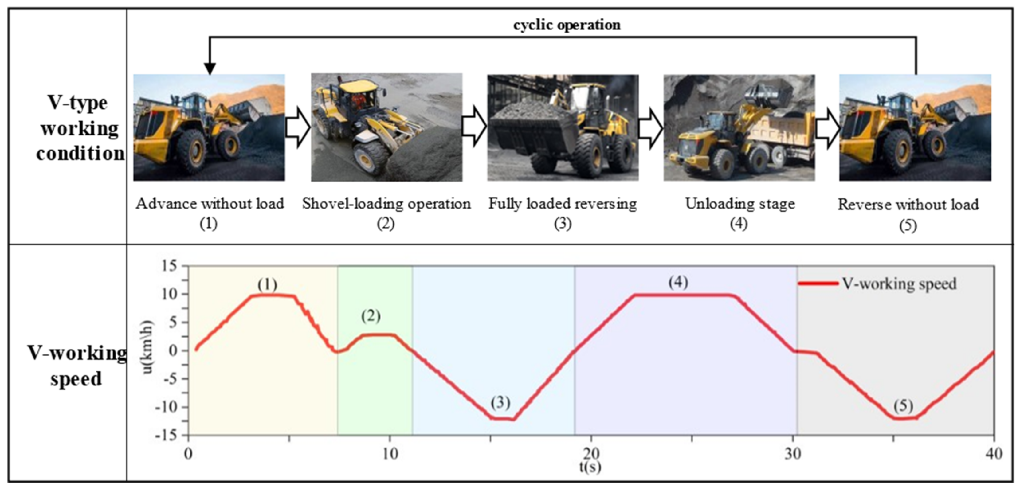
The whole V-type operation cycle of the loader can also be divided into five phases, which include (1) the empty-load forward phase, (2) the shoveling operation phase, (3) the full-load reversing phase, (4) the unloading phase, and (5) the unloaded reversing phase. When the unloading is completed, the reversing vehicle is returned to the original position to continue the next round of shoveling operation [16], as shown in Figure 2.
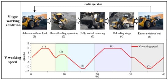
Figure 2.
Loader V working mode.
As shown in Figure 3b, the loader’s motion necessitates adhering to the dynamic equilibrium equation, where the tractive force of the loader must overcome rolling resistance , incline-induced slope resistance , aerodynamic drag , and the inertia resistance during acceleration [17]. In Figure 3a, when the loader is engaged in V-shaped operational work, it needs to overcome loading resistance . This resistance can be divided into three components: insertion resistance , digging resistance , and bucket rotation resistance [18,19,20]. In the operational process of the loader, the external load is subject to variation. To more accurately simulate real-world conditions, the loader’s vehicle model from the component library was used as the load model, and the load parameters were defined as presented in Table 2. This model enables parameter adjustments such as mass and digging resistance during the loader’s operational process, ensuring that the simulation settings closely resemble actual conditions.
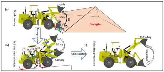
Figure 3.
V-shaped working mode force situation: (a) Shovel loading operation, (b) Transportation and lifting operations, and (c) Unloading and reshovel loading operations.
Table 2.
Load model parameters.
The model of tires used for the drive wheels is 17.5–25, and the tire radius is m. Thus, when achieving the maximum vehicle speed , the wheel speed can be calculated using Equation (13). With the gear ratio determined, the maximum speed of the two motors can be derived. Under the rated speed, choosing a pump displacement of 175.4 mL/r satisfies the system flow rate requirement.
The resistance and maximum power required by for typical road conditions are shown in Table 3 [21].
Table 3.
Typical road resistance and maximum power.
Table 3 indicates that the highest power demand occurs on a sloped road surface (30°), with equating to 145.35 kW. Assuming an overall transmission efficiency of 0.85 and accounting for power losses associated with the static hydraulic transmission system, the engine power Pe should not fall below 171 kW. Typically, for loader vehicles, the engine is rated within the range of 1500 to 2000 rpm [22]. In construction vehicles, the hydraulic components’ rated pressure for travel () is typically set at 0.45- to 0.65-times the highest calibration pressure () and the maximum relief pressure () is suitable at 0.8 [23]. Based on past design experience, setting at 42 MPa for the 7-ton loader satisfies the requirements.
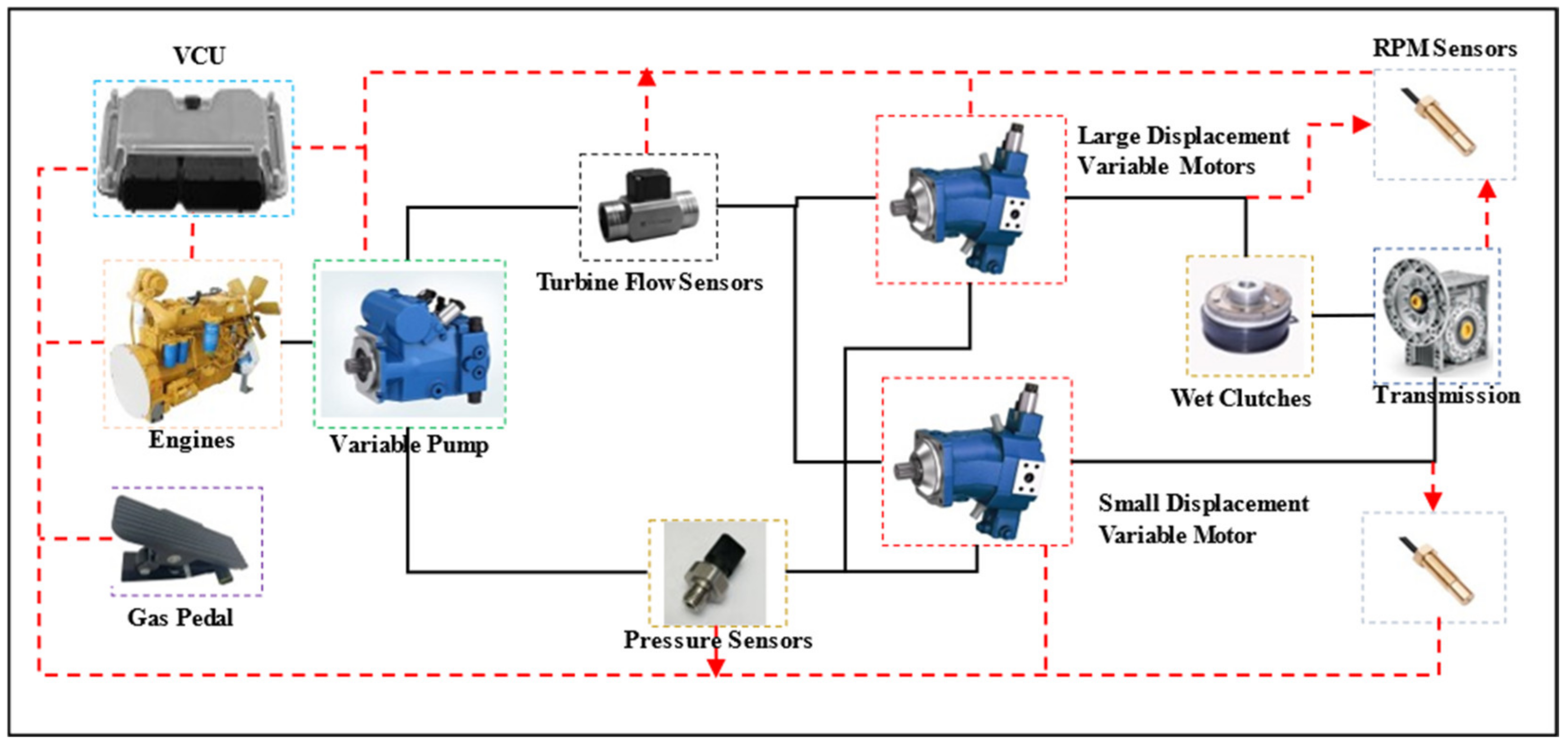
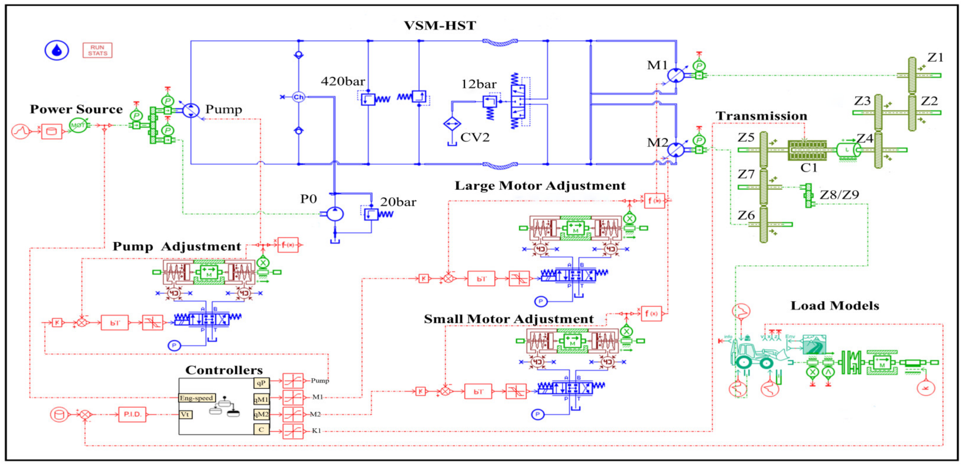
Based on the components and layout of the system in Figure 1, the actual system components were selected according to the design parameters in Table 4, as shown in Figure 4. The system was further modeled for simulation using AMESIM software (AMESIM 22.1 version), as shown in Figure 5.
Table 4.
Simulation model parameters.

Figure 4.
VSM-HST system main components and layout, the red dash line shows the electrical signal transmission path, the red dash arrow shows the direction of unidirectional electrical signal transmission, and the black full line shows the mechanical signal transmission path.
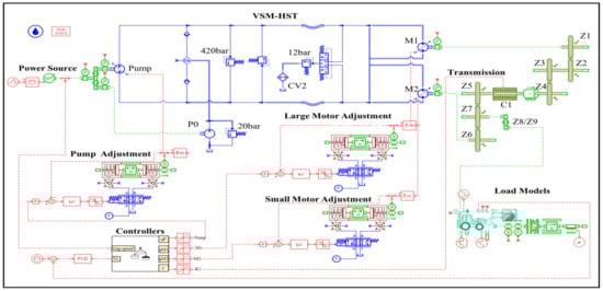
Figure 5.
Simulation model of VSM-HST, the blue color represents the hydraulic system, the green color represents the mechanical system, the red color represents the signaling system, and the yellow color represents the input and output ports.
3. Control Strategy
To control the vehicle’s proficiently, an MCF–SMC control strategy is proposed. Through real-time detection of gas pedal changes, this system determines the driver’s intended operation and generates a target speed signal based on the current driving speed [24,25].
3.1. Mathematical
Models
Therefore, it is essential to establish equations that relate the system’s various parameters to the displacement states. Considering that motor displacement changes are in the opposite direction to the control logic, M1-controlled displacement and M2-controlled displacement are introduced. Their relationships with actual displacements are given by Equation (14) and Equation (15), respectively:
The actual displacement of the pump and the controlled displacements of the two motors in the system vary proportionally with the increase in the displacement control signal. The relationships between displacement and control signal are given by Equations (16)–(18):
where and represent the time and proportionality constants of the variable pump. and and and indicate the time and proportionality constants of M1 and M2, respectively.
To ensure control accuracy, it needs to account for the effects of system leakage, inertia, and damping. Combining the analysis of various parameters from Section 2.2, the flow balance equation and torque balance equation for the system can be derived. These equations are given by Equations (19) and (20):
where , P, and denote the total leakage coefficient of the pump, the outlet pressure, and the total volume of the high-pressure chamber side, respectively, and represent the total leakage coefficients of M1 and M2, respectively, and is the modulus of elasticity of the hydraulic fluid.
The load torque balance equation for a variable motor is Equation (20):
where is the load moment of inertia, is the damping factor, and is the load torque. Let , so the association of Equation (14) to Equation (20) and the collation leads to the system’s state equation as Equation (21).
where the coefficients are
Equation (21) indicates that , , , and have a nonlinear correlation, highlighting the hydrostatic dual-motor circuit as a three-input single-output nonlinear system with inputs of , , and and an output of . The state Equation (21) simplifies to Equation (22):
where represents the nonlinear state function matrix, () corresponds to the input gain function matrix, is the output function matrix, and denotes the external perturbation matrix.
3.2. MCF–SMC
The MCF–SMC control strategy comprises Sliding Mode Control (SMC) and Multivariable Fuzzy Control (MCF). The following explanations are based on the system’s dynamic equations derived in Section 3.1. The first-order differentiation of in Equation (22) gives the output as a function of the three inputs as in Equation (23).
When is fixed, the inputs , , and all affect the output of the vehicle’s speed. However, based on the analysis of the control characteristics in Section 2.2, it is determined that in different speed ranges of the loader, only one input has the maximum influence on the output. Therefore, the vehicle speed is segmented into ranges, with one primary input dominating each range, while the other inputs remain constant and are deemed disturbances that have no impact on the vehicle’s speed. Specifically, when , the dominant input is ; when , the dominant input is ; and when , the dominant input is . This relationship is expressed by Equation (24):
SMC, a nonlinear control technique, employs the real-time state of the system and experiences continuous regular changes to steer complex nonlinear systems by enforcing a desired state trajectory, referred to as the sliding mode surface. This approach delivers effective control performance with high-frequency and small fluctuations. To implement this method, two tasks must be completed: designing the sliding mode surface for the system and designing a control law that will move the system state to the sliding mode surface.
The tracking error is the difference between the ideal vehicle speed and the actual vehicle speed , as shown in Equation (22).
According to Equation (21), the sliding mode surface is defined as Equation (26).
where and are constants greater than zero whose values can be determined by having pole configurations that satisfy the requirements of the Laws criterion [26].
From Equations (22)–(26), the system control rate can be derived as shown in Equation (27).
where is the a priori expected speed, , .
The in Equation (27) is indeterminate. To ensure a smooth reaching of the system state to the sliding mode surface, the design of the convergence rate also needs to adapt to the external perturbation. In this paper, an exponential convergence rate was adopted, as shown in Equation (28).
where , and are constants greater than zero, whose magnitude determines the switching and convergence speeds. Because the time constants of the pumps and motors are 0.1 s, let . From Equations (27) and (28), the final system sliding mode control rate is Equation (29).
where is the approximation function of as shown in Equation (27), and is the compensation function about , and good robustness and stability of the system can be realized by controlling the values of and reasonably.
In control theory, the Lyapunov function is used to determine the stability of the system [27]. For the control objective , if there exists a continuous function that satisfies Equations (30) and (31), the system will be stable at the equilibrium point , that is .
Let , which clearly satisfies the first condition of Lyapunov stability [28]. Taking the derivative of yields:
When , the system satisfies the second condition of Lyapunov stability, so the system will eventually stabilize near the sliding mode surface, and the two variables will eventually reach equilibrium.
But for practical engineering problems, the time required for stability and the stability after interference also need to be considered. It has been proven above that the system is stable, so let directly, where represents the upper limit of system error and the proof process is as follows:
The above equation proves that the system will reach stability within a finite time, and the stability time is:
Therefore, it is necessary to add a constraint to as Equation (34).
When the system is affected by external interference , where is the upper bound of the interference [29], then there is Equation (35)
In summary, under the condition of meeting the limited conditions, through reasonable control, the values of and can achieve good robustness and stability of the system.
MCF is a rule-based control algorithm that, when combined with SMC, can minimize jitter resulting from abrupt and rapid system parameter adjustments. The input variables for MCF are and , representing the relative distances between the state point and the sliding mode surface and the state point’s speed relative to the sliding mode surface, respectively. The output quantity, is adjusted based on the fuzzy rules that guarantee the establishment of . The linguistic variables and their ranges were selected as {−3 −2 −1 0 1 2 3} for both the controller’s input and output. The associated linguistic terms for these variables are NB, NM, NS, ZO, PS, PM, and PB, which stand for Negative Big, Negative Medium, Negative Small, Zero, Positive Small, Positive Medium, and Positive Big, respectively. The controller’s input–output mapping applies triangular membership functions to the linguistic terms by the design guidelines outlined in references [30,31,32]. An illustration of these triangular membership functions can be found in Figure 6.

Figure 6.
Triangular affiliation function.
The control logic equation is formulated as shown in Equation (30).
The paper utilizes the widely accepted weighted average method for defuzzification, which has been previously outlined in studies [33,34,35]. Equation (31) presents the calculation formula for this method.
where is the defuzzification value, is the value of the affiliation function, and is the center of mass of the affiliation function. Under the condition that the inequality is met, the control rules for the output variable ε were designed based on empirical knowledge, as illustrated in Table 5.
Table 5.
Switching speed fuzzy control rules.
Due to the variable-structure nature of the VSM-HST system involving structural switching, in conjunction with the analysis of operational conditions, the automatic shifting mode was divided into low-speed mode and high-speed mode based on the transition of the transmission structure. When the vehicle transitions from low-speed mode to high-speed mode, the transmission structure shifts automatically, ensuring a smooth transition of speed ranges. However, drivers can switch between these modes manually. Typically, the low-speed mode is utilized for loading, short-distance transport and heavy transportation, while the high-speed mode is reserved for long-distance transport and high-speed travel. The vehicle starts in the low-speed mode by default. In this mode, both M1 and M2 operate simultaneously, with M2 maintaining maximum displacement. When the driver enables travel, the vehicle moves at idle speed, with the pump set to minimum displacement and the motor maintaining maximum displacement, resulting in a travel speed of 1 km/h. Upon receiving a signal indicating an increase in throttle pedal movement, the engine speed gradually increases until the rate of change becomes zero.
As engine speed increases, pump displacement also increases, resulting in a gradual increase in travel speed. At the same time, M1 displacement decreases in response to the increase in speed, further enhancing travel speed. This process continues until the system stabilizes and the desired travel speed is achieved within an acceptable margin of error. If a further increase in travel speed is required, the system will automatically exit the low-speed mode and enter the high-speed mode. As M1’s displacement approaches zero, the clutch disengages between M1 and the output shaft. Decreasing M2’s displacement further increases the travel speed. Once M2’s displacement reaches the set minimum, the pump attains maximum displacement. The control logic’s schematic representation is shown in Figure 7.
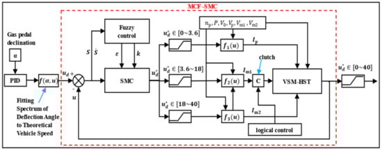
Figure 7.
MCF–SMC control logic schematic.
3.3. Simulation Results
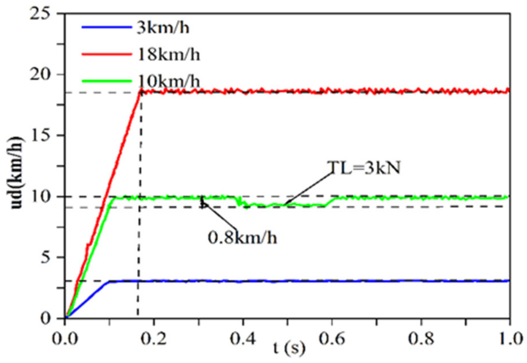
In the simulation scenario with a load of , constant engine speed , and other parameters remaining the same, three different target speeds were set: 3 km/h, 10 km/h, and 18 km/h. An additional impact load of was applied at 0.4 s of the simulation for the experimental group with a target vehicle speed of 10 km/h.
This simulation was carried out under ideal conditions, where the control current range for both the pump and motors was within (−400 mA, 400 mA). The displacement control signals can be directly controlled by amplifying the current through a current amplifier or a similar mechanism. The MCF–SMC parameters are provided in Table 6.
Table 6.
MCF–SMC parameters.
The results are shown in Figure 8. The simulation results demonstrate that the control strategy effectively tracks and predicts the target speeds. In the presence of a sudden 3 kN load disturbance, the speed variation is around 0.8 km/h, which is less than 1 km/h. Furthermore, the speed quickly returns to the target value after the disturbance disappears, indicating that the control strategy can handle load disturbances well and ensure the stability of the system control.

Figure 8.
Control strategy simulation results.
To assess the efficacy of the MCF–SMC, simulations were conducted and its performance to typical control algorithms employed in electro-hydraulic servo systems was compared. Figure 9 illustrates the actual speed output curve obtained at an external load of , an engine speed of , and a target speed of .
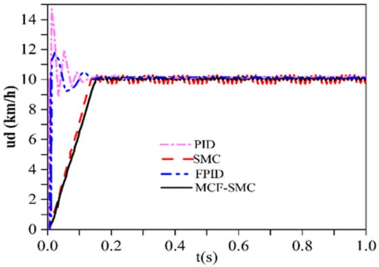
Figure 9.
Algorithm comparison experiment results.
In the simulation comparison test, the pre-experimental control algorithm only replaced the fuzzy control and SMC parts depicted in Figure 7. The control logic and VSM-HST settings were unaltered. During the experiment, severe overshoot was observed in numerous experiments when using the PID algorithm. After implementing the widely-used integral separation and anti-integral saturation methods, the system was still affected, although to a lesser degree, by overshoot, and the PID control output generated the vehicle speed curve illustrated in Figure 9. The PID was further enhanced with the fuzzy control strategy. The integral coefficient in the variable integral strategy was adjusted based on deviation size. Faster integration occurs for smaller deviations, while slower integration takes place for larger deviations. If the deviation surpasses a specific threshold, the integral term is set to zero. The resulting FPID experimental curve is represented in Figure 9. Despite numerous attempts to debug, the vehicle’s speed output still experiences oscillations during the initial start-up phase. The use of SMC control eliminates initial stage oscillations, but small amplitude oscillations persist near the target vehicle speed after system convergence. Incorporating a fuzzy control strategy effectively suppresses these vibrations, improving control quality. MCF–SMC appears to be a more suitable strategy for VSM-HST system control compared to other alternatives.
4. Experimental Verification
To check the performance of the VSM-HST system and MCF–SMC control strategy. In this paper, the simulation results obtained from the ideal state were compared with the processed test results to determine whether the system and control strategy can meet the demands of the loader in actual V-type operation cycle conditions.
4.1. Experimental Design
The experimental process and equipment are shown in Figure 10. The Liu Gong 886H hydrostatic loader was selected for the V-shaped operation cycle test. The key parameters of the main hydraulic components are given in Table 3. The vehicle controller used is the standard configuration of Liu Gong’s series products, and the experimental data sampling time was set to be 0.5 s. The experimental process is as follows:
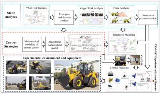
Figure 10.
Experimental procedure and equipment.
- (1)
- The speed sensor was installed in the rear-wheel-drive shaft of the loader, and the variable pump input shaft was installed in two places. The pressure and flow sensors were installed in the hydraulic circuit, and the formulated control strategies and algorithms were written into the VCU controller. The sensors were connected to the controller, which was connected to the collector through the CAN2.0B bus. The controller was connected to the collector via the CAN2.0B bus.
- (2)
- The loader began from the initial position and accelerated by stepping on the accelerator pedal. It maintained a constant speed in the middle by controlling the accelerator pedal before releasing it near the pile. The loader stopped by using the resistance of the pile and then increased the accelerator pedal to shovel the load. Once the shoveling was complete, it drove in reverse by first accelerating and then reversing. After shoveling, the vehicle was reversed, first accelerating and then decelerating to the starting position, and then driving in the right direction to the loading truck, first accelerating and then decelerating to the loading truck for unloading. After unloading, the vehicle was reversed, first accelerating and then decelerating back to the home position. During this operation, the engine speed, wheel speed, system pressure, system flow, pump, and engine displacement of the loader were collected and recorded.
- (3)
- This procedure was repeated multiple times to ensure a consistent collection of experimental data.
4.2. Experimental Results
The loader’s total completion time for the V-type operation condition is approximately 40 s. This test was conducted three times initially, and after idling for 15 s in the middle, the V-type operation was carried out three additional times, resulting in a total of six groups for the experiment with a combined duration of approximately 283 s.
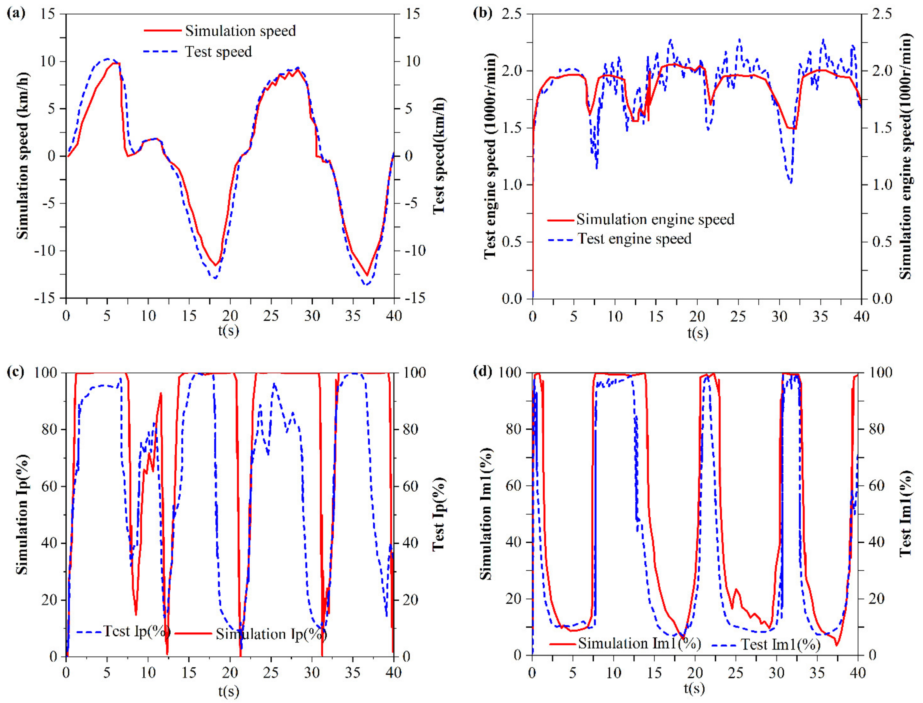
To visualize the actual operation more, the six sets of experimental data were averaged and analyzed in comparison with the simulation data. From Figure 11a, it can be seen that the actual speed of the loader can track the target speed well. Figure 11b shows that the diesel engine can reach the rated speed near 2000 r/min quickly after starting and can return to the idling speed quickly when braking.
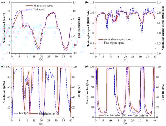
Figure 11.
Speed tracking situation: (a) Actual vehicle speed versus expected target vehicle speed tracking, (b) Actual engine speed versus control speed tracking, (c) Comparison between actual and expected pump displacement, and (d) Comparison between actual and expected displacement of motor M1.
Figure 11c,d display changes in the proportion of the variable pump and large motor displacement ratios. At the onset of the loader’s operation, the simulated flow rate of the variable pump surpasses the actual flow rate delivered.
When the engine speed reaches approximately 2000 rpm, following the completion of the loader’s start-up process, the errors in the simulation results and the test results for the pump displacement ratio and the large motor displacement ratio are minimal. As the loader decelerates, the errors in the pump displacement ratio and the large motor displacement ratio increase. During the shoveling phase, the errors in the pump and large motor displacement ratios are relatively small. In the full-load start-up stage, the pump displacement ratio errors increase, while the large motor displacement ratio error remains within acceptable limits. In the full-load acceleration stage, the simulation and test results indicate that the pump displacement ratio errors reach their maximum value, with the large motor displacement ratio error increasing. In the full-load deceleration stage, the pump displacement ratio errors become more significant, exceeding acceptable limits, while the large motor displacement ratio error remains within 20%.
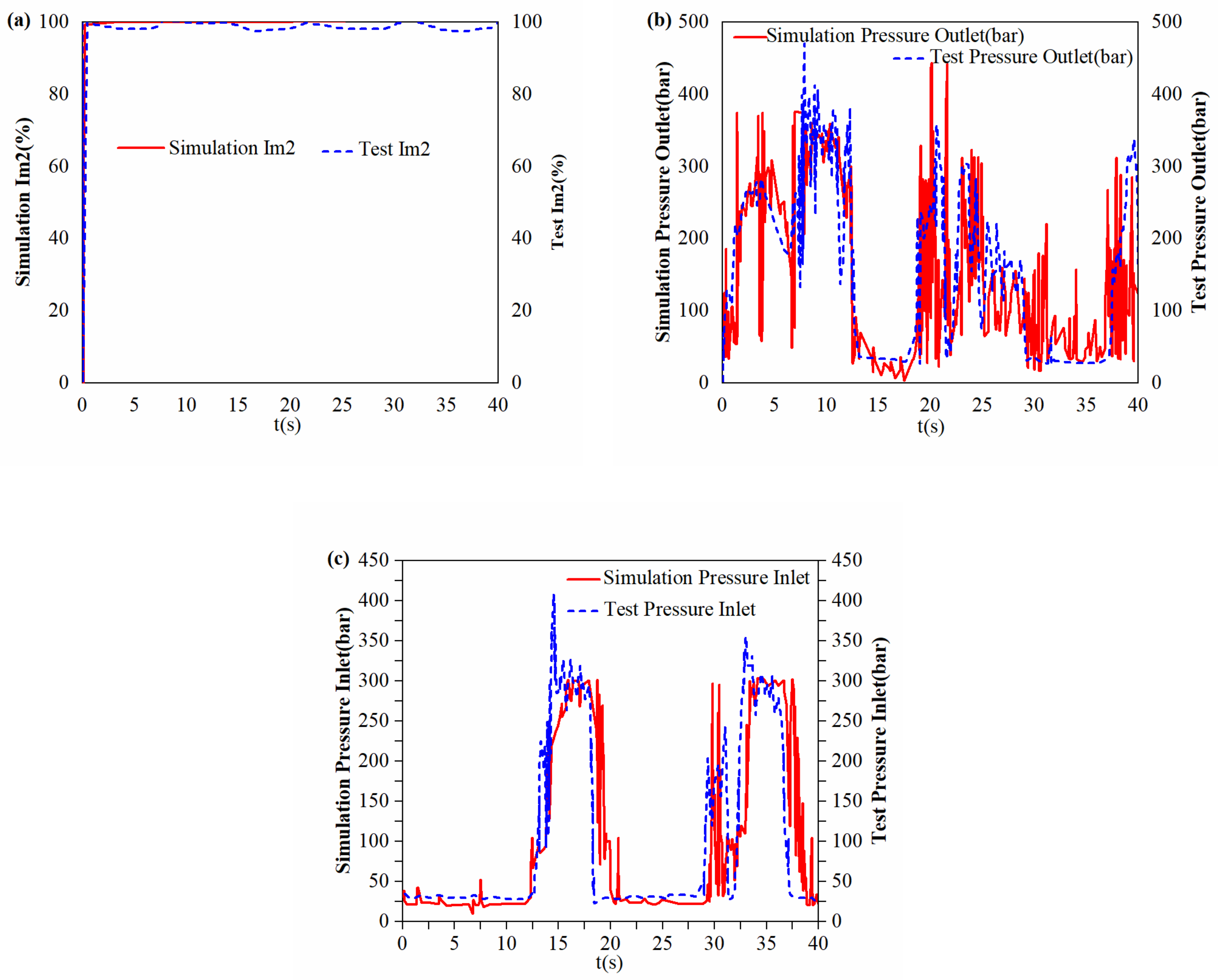
The change in the ratio of the small motor displacement fluctuates slightly around the desired value, as shown in Figure 12a. Figure 12b,c show the simulation results of the pump inlet pressure and pump outlet pressure changes with the test results, respectively, as the error is larger in 8–12 s as the test data fluctuate more drastically, mainly because the bucket will shake during the shoveling process, and the shoveling resistance will change during the shoveling process, which leads to fluctuation of the test data, resulting in error; during the experiment, the loader was driven in reverse during the period of 12–18 s, and at this time, the pump inlet pressure was always higher than the pump outlet pressure. When the loader is fully loaded, from 0 to 8 s, the pressure value exceeds that of the hydrostatic system.
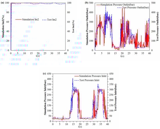
Figure 12.
Small motor displacement and pressure, (a) Comparison between actual and expected displacement of motor M2, (b) Comparison between experimental and simulated values of pump outlet pressure in closed hydraulic systems, and (c) Comparison between experimental and simulated values of pump inlet pressure in closed hydraulic systems.
The error in this part of the data is within 10%. During the 18 to 29 s period, the loader is fully loaded and moving forward to load, and the pump discharge pressure is always higher than the pump inlet pressure. During the period from 29 to 40 s, the loader is in a no-load state for reversing at this time and the pump inlet pressure is always higher than the pump outlet pressure. It is observed from comparing the parameter changes above that the simulation results of each parameter are consistent with the test data trend. This proves that the speed control strategy satisfies the V-type operating conditions of the loader.
4.3. Experimental Discussion
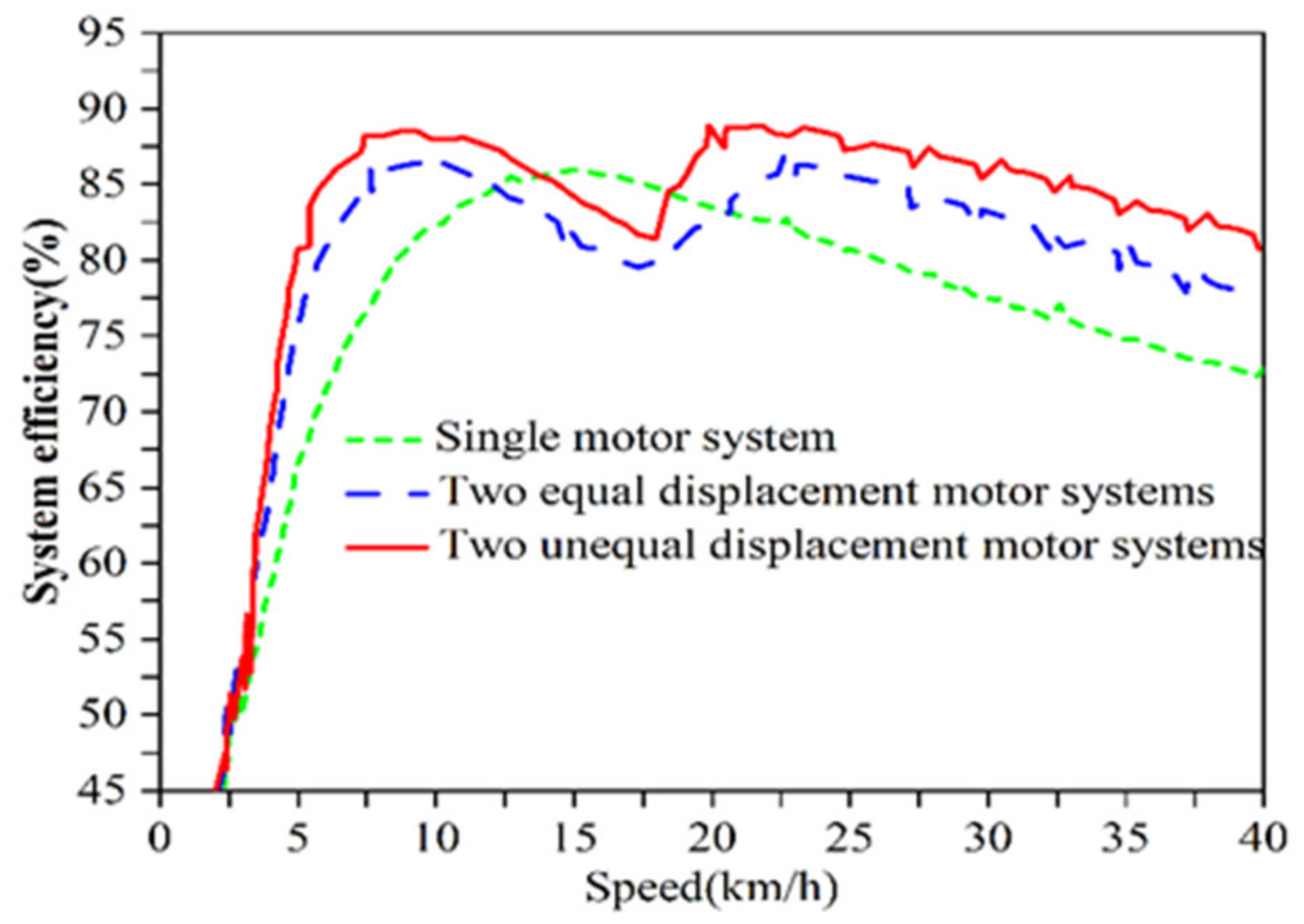
To demonstrate the performance of our designed VSM-HST system, simulation experiments were conducted comparing three different design schemes of VPVMS. While ensuring consistent parameters and components, the same variable pump station was used to supply oil to a single-variable motor, two variable motors with equal maximum displacement, and the VSM-HST system simultaneously. The efficiency curves of the three schemes are shown in Figure 13.
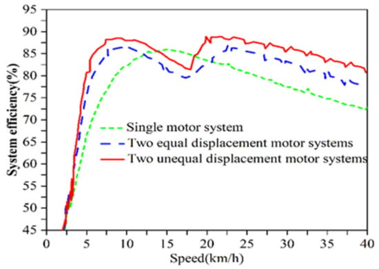
Figure 13.
Efficiency curves for the three scenarios. This figure shows the power efficiency of different systems simulated after modifying a single configuration using the same loader equipped with VSM-HST system to complete the same task. The green dashed line indicates the efficiency of always shutting down one motor of the VSM-HST system and completing tasks with only a single motor. The blue dashed line represents the efficiency of completing tasks by always ensuring that the initial displacement and displacement changes in the two motors in the VSM-HST system are the same. The red dashed line indicates the efficiency of completing tasks using the VSM-HST system normally.
In the low-speed, high-torque working condition (0–4.7 mph), system efficiency is lower as the pump operates in a zone of low efficiency with high system pressure and notable leakage. However, efficiency increases rapidly at higher speeds. When the vehicle speed is between 7.5 and 17.5 km/h, the efficiency of both the dual-equal displacement motors and dual-variable displacement motors decreases with increasing speed due to the reduction in displacement of the two motors. The VSM-HST system provides higher efficiency throughout the entire speed range of the loader, along with a wider speed range of high efficiency. Additionally, the advantages of the VSM-HST system are more pronounced while handling larger loads and higher velocities.
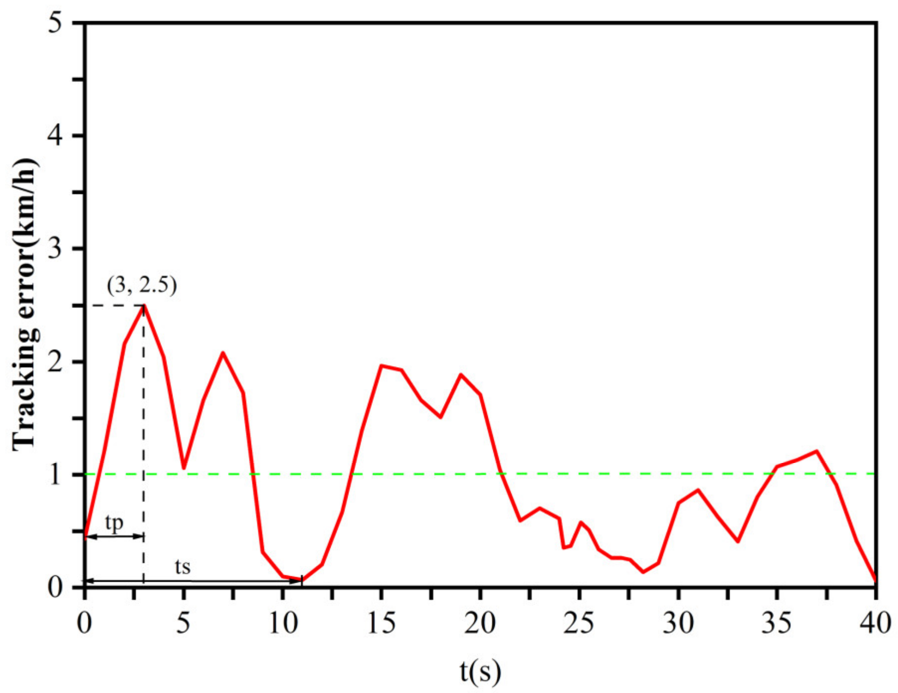
Figure 14 shows the change in tracking error value of the loader complete for the V-type working process in the field test, and the average error of the whole process is 1 km/h, and the maximum error is 2.5 km/h. Because the target value changes during the whole process, the loader was started from the initial speed of zero to the shoveling of materials to complete the stabilization of the loader as a typical section to illustrate the transient performance of the loader, and the overshoot time of this stage was , and the whole process regulation time was . Compared to the HST scheme and its control strategy introduced earlier, the VSM-HST and MCF–SMC schemes have different layouts and structural designs and consider multivariable collaborative controls. They have the following advantages.

Figure 14.
Field experiment tracking error curve where denotes the overshoot time, denotes the regulation time, red solid line denotes the error curve, and green dashed line denotes the average error value.
- (a)
- The VSM-HST has the advantages of a more compact structure, a wider high-efficiency speed range, and higher total efficiency. It can directly transplant and replace the hydraulic traveling mechanism of traditional construction machinery and apply it to the whole product line.
- (b)
- MCF–SMC is specially designed for the VSM-HST system, which successfully realizes the overall control of multiple variables, effectively adapts to and controls the sudden change in speed caused by load change during the actual operation of wheel loader, and ensures the smoothness of the speed regulation process. It effectively overcomes the challenges posed by the time delay and nonlinearity of the hydraulic system and ensures the driving quality.
- (c)
- The VSM-HST and MCF–SMC solutions enable smooth, stepless automatic gear shifting over the entire speed range of the wheel loader, with free selection of high and low gears. The main components within the system are controllable, which greatly enhances the control potential of the system and facilitates intelligent retrofitting, especially for vehicle speed control of driverless construction machinery.
Any system has limitations, and the efficiency gains of the designed VSM-HST system are not significant at low speeds and heavy loads, which may be because the overall efficiency gains are hampered by the fact that both the fuel efficiency of the engine and the volumetric efficiency of the pumps are low when the vehicle is started.
5. Conclusions
This study aims to improve the working efficiency of the loader transmission system and reduce fuel consumption. A novel VSM-HST system is proposed, and an adaptive improvement is made to the fuzzy sliding mode control strategy for the control problems of this system, proposing an MCF–SMC control method.
Combining a theoretical analysis, a working condition analysis, a simulation analysis, and an experimental analysis, the performance and application scenarios of the proposed new loader transmission system are explained, and the following conclusions are drawn:
- (1)
- The proposed VSM-HST system can meet the speed requirements of different road conditions under the V-shaped working mode of the loader. The adjustment process is smooth, and the speed switching is smooth.
- (2)
- The proposed MCF–SMC control strategy can match the system well. The test proves that the maximum tracking error of the target speed is only 2.5 km/h under normal driving conditions, and the average deviation of the speed is 1 km/h when subjected to an external disturbance load not exceeding the rated load. A good control effect is achieved within the allowable error range.
- (3)
- Compared with loaders using traditional hydrodynamic torque converter transmission systems, under the same initial conditions and operating conditions, the total efficiency of the VSM-HST system is increased by about 30%, and the total efficiency is increased by about 8% compared to other traditional HST schemes. This shows that this scheme can effectively improve transmission efficiency and reduce fuel consumption.
In the future, we will further optimize the control algorithm, use intelligent algorithms, such as deep neural networks or Radial Basis Function Neural Networks (RBF) to compensate for the impact of uncertain factors, or use meta-learning ideas to design super-heuristic intelligent control algorithms to further improve system performance.
Author Contributions
Conceptualization, W.M.; Methodology, L.X.; Software, L.X.; Validation, L.X.; Formal analysis, S.W.; Investigation, Z.W. (Zhongshan Wang); Resources, Z.W. (Zhongshan Wang); Data curation, Z.W. (Zhongyu Wang) and L.X.; Writing—original draft, Z.W. (Zhongyu Wang); Writing—review & editing, X.W.; Visualization, Z.W. (Zhongyu Wang) and L.X.; Supervision, X.W., S.W. and W.M.; Project administration, X.W. and W.M.; Funding acquisition, X.W. and W.M. All authors have read and agreed to the published version of the manuscript.
Funding
Guangxi Key Research and Development Program: Research on Key Technologies for Energy Saving in Intelligent Static Hydraulic Transmission of Wheel Loaders (Guike AB22080041).
Data Availability Statement
The datasets supporting the conclusions of this article are included within the article.
Conflicts of Interest
Author Lei Xie was employed by the Huawei Terminal Co., Ltd. Author Songlin Wang was employed by the Guangxi Liu Gong Machinery Co., Ltd. The remaining authors declare that the research was conducted in the absence of any commercial or financial relationships that could be construed as a potential conflict of interest.
References
- Frank, B.; Kleinert, J.; Filla, R. Optimal control of wheel loader actuators in gravel applications. Autom. Constr. 2018, 91, 1–14. [Google Scholar] [CrossRef]
- Nezhadali, V.; Frank, B.; Eriksson, L. Wheel loader operation—Optimal control compared to real drive experience. Control Eng. Pract. 2016, 48, 1–9. [Google Scholar] [CrossRef]
- Nilsson, T.; Fröberg, A.; Åslund, J. Development of look-ahead controller concepts for a wheel loader application. Oil Gas Sci. Technol. 2015, 70, 159–178. [Google Scholar] [CrossRef]
- You, Y.; Sun, D.; Qin, D. Shift strategy of a new continuously variable transmission based wheel loader. Mech. Mach. Theory 2018, 130, 313–329. [Google Scholar] [CrossRef]
- Lin, T.; Wang, Q.; Hu, B.; Gong, W. Development of hybrid powered hydraulic construction machinery. Autom. Constr. 2010, 19, 11–19. [Google Scholar] [CrossRef]
- Wang, F.; Chen, J.; Xu, B.; Stelson, K.A. Improving the reliability and energy production of large wind turbine with a digital hydrostatic drivetrain. Appl. Energy 2019, 251, 113309. [Google Scholar] [CrossRef]
- Xupeng, H.; Wenbin, S.; Hang, Z.; Yanni, Z.; Qiao, H.; Chaohui, W. Research of the hydrostatic transmission for deep-sea current energy converter. Energy Convers. Manag. 2020, 207, 112544. [Google Scholar] [CrossRef]
- Comellas, M.; Pijuan, J.; Nogués, M.; Roca, J. Efficiency analysis of a multiple axle vehicle with hydrostatic transmission overcoming obstacles. Veh. Syst. Dyn. 2018, 56, 55–77. [Google Scholar] [CrossRef]
- Rabbo, S.A.; Tutunji, T. Identification and analysis of hydrostatic transmission system. Int. J. Adv. Manuf. Technol. 2008, 37, 221–229. [Google Scholar] [CrossRef]
- Backas, J.; Ghabcheloo, R.; Huhtala, K. Gain scheduled state feedback velocity control of hydrostatic drive transmissions. Control Eng. Pract. 2017, 58, 214–224. [Google Scholar] [CrossRef]
- Do, H.T.; Park, H.G.; Ahn, K.K. Application of an adaptive fuzzy sliding mode controller in velocity control of a secondary controlled hydrostatic transmission system. Mechatronics 2014, 24, 1157–1165. [Google Scholar] [CrossRef]
- Schulte, H.; Gauterin, E. Fault-tolerant control of wind turbines with hydrostatic transmission using Takagi–Sugeno and sliding mode techniques. Annu. Rev. Control 2015, 40, 82–92. [Google Scholar] [CrossRef]
- Jiang, W.; Zhang, C.; Jia, P.; Yan, G.; Ma, R.; Chen, G.; Ai, C.; Zhang, T. A Study on the Electro-Hydraulic Coupling Characteristics of an Electro-Hydraulic Servo Pump Control System. Processes 2022, 10, 1539. [Google Scholar] [CrossRef]
- You, Y.; Sun, D.; Qin, D.; Wu, B.; Feng, J. A new continuously variable transmission system parameters matching and optimization based on wheel loader. Mech. Mach. Theory 2020, 150, 103876. [Google Scholar] [CrossRef]
- Cao, B.W.; Liu, C.Y.; Chen, W.; Tan, P.; Yang, J.W. Shovel-loading cooperative control of loader under typical working conditions. ISA Trans. 2023, 142, 702–715. [Google Scholar] [CrossRef] [PubMed]
- Wang, F.; Wen, Q.; Xu, X.; Xu, B.; Sun, Z. Site Operation Strategy for Wheel Loader/Truck Loading and Transportation Cycle. IEEE Trans. Veh. Technol. 2021, 70, 4129–4138. [Google Scholar] [CrossRef]
- Ur Rehman, A.; Awuah-Offei, K. Understanding How Speed, Tractive Effort, Digging Height, and Rake Angle Affect Bucket Penetration and Resistive Forces for Rubber Tire Loaders. Min. Metall. Explor. 2020, 37, 1423–1435. [Google Scholar] [CrossRef]
- Wu, B.; Hou, L.; Wang, S.; Yin, Y.; Yu, S. Predictive modeling of loader’s working resistance measurement based on multi-sourced parameter data. Autom. Constr. 2023, 149, 104805. [Google Scholar] [CrossRef]
- Takahashi, H.; Hasegawa, M.; Nakano, E. Analysis on the resistive forces acting on the bucket of a Load-Haul-Dump machine and a wheel loader in the scooping task. Adv. Robot. 1998, 13, 97–114. [Google Scholar] [CrossRef]
- Yuan, Z.; Lu, Y.; Hong, T.; Ma, H. Research on the load equivalent model of wheel loader based on pseudo-damage theory. Proc. Inst. Mech. Eng. Part C J. Mech. Eng. Sci. 2022, 236, 1036–1048. [Google Scholar] [CrossRef]
- Gao, G.; Wang, J.; Ma, T.; Han, Y.; Yang, X. Optimisation strategy of torque distribution for the distributed drive electric wheel loader based on the estimated shovelling load. Veh. Syst. Dyn. 2022, 60, 2036–2054. [Google Scholar] [CrossRef]
- Tan, P.; Liu, X.-H.; Liu, C.-Y.; Zhang, C.; Chen, W.; Cao, B.-W.; Yang, K.; You, T. Investigating the matching characteristic of the full hydraulic braking system of the wheel loader. J. Braz. Soc. Mech. Sci. Eng. 2022, 44, 209. [Google Scholar] [CrossRef]
- Wu, H.W.; Lee, C.B. Influence of a relief valve on the performance of a pump/inverter controlled hydraulic motor system. Mechatronics 1996, 6, 1–19. [Google Scholar] [CrossRef]
- Huang, J.; Cheng, X.; Shen, Y.; Kong, D.; Wang, J. Deep Learning-Based Prediction of Throttle Value and State for Wheel Loaders. Energies 2021, 14, 7202. [Google Scholar] [CrossRef]
- Ma, W.; Zhang, Y.; Liu, C.; Wang, S. Prediction Method of the Fuel Consumption of Wheel Loaders in the V-Type Loading Cycle. Res. Artic. 2015, 2015, 538176. [Google Scholar] [CrossRef]
- Singh, V. A note on Routh’s criterion and Lyapunov’s direct method of stability. Proc. IEEE 1973, 61, 503. [Google Scholar] [CrossRef]
- Cerman, O.; Hušek, P. Adaptive fuzzy sliding mode control for electro-hydraulic servo mechanism. Expert Syst. Appl. 2012, 39, 10269–10277. [Google Scholar] [CrossRef]
- Chiang, M.-H.; Lee, L.-W.; Liu, H.-H. Adaptive Fuzzy Controller with Self-tuning Fuzzy Sliding-mode Compensation for Position Control of an Electro-hydraulic Displacement-controlled System. J. Intell. Fuzzy Syst. 2014, 26, 815–830. [Google Scholar] [CrossRef]
- Zhang, J.; Chen, D.; Shen, G.; Sun, Z.; Xia, Y. Corrigendum to “Disturbance observer based adaptive fuzzy sliding mode control: A dynamic sliding mode surface approach” [Automatic 129 (2021) 109606]. Automatic 2022, 142, 110413. [Google Scholar] [CrossRef]
- Lu, Y. Adaptive-Fuzzy Control Compensation Design for Direct Adaptive Fuzzy Control. IEEE Trans. Fuzzy Syst. 2018, 26, 3222–3231. [Google Scholar] [CrossRef]
- Abbasi, S.M.M.; Jalali, A. Fuzzy tracking control of fuzzy linear dynamical systems. ISA Transactions 2020, 97, 102–115. [Google Scholar] [CrossRef] [PubMed]
- Killian, M.; Mayer, B.; Schirrer, A.; Kozek, M. Cooperative Fuzzy Model-Predictive Control. IEEE Trans. Fuzzy Syst. 2016, 24, 471–482. [Google Scholar] [CrossRef]
- Mustafa, A.M.; Gong, Z.; Osman, M. Fuzzy Optimal Control Problem of Several Variables. Adv. Math. Phys. 2019, 2019, 2182640. [Google Scholar] [CrossRef]
- Phu, N.D.; Van Tri, P. The Fuzzy Dynamic Programming Problems. J. Intell. Fuzzy Syst. 2016, 30, 1663–1674. [Google Scholar] [CrossRef]
- Zhao, Y.; Zhu, Y. Fuzzy optimal control of linear quadratic models. Comput. Math. Appl. 2010, 60, 67–73. [Google Scholar] [CrossRef]


Disclaimer/Publisher’s Note: The statements, opinions and data contained in all publications are solely those of the individual author(s) and contributor(s) and not of MDPI and/or the editor(s). MDPI and/or the editor(s) disclaim responsibility for any injury to people or property resulting from any ideas, methods, instructions or products referred to in the content. |
© 2024 by the authors. Licensee MDPI, Basel, Switzerland. This article is an open access article distributed under the terms and conditions of the Creative Commons Attribution (CC BY) license (https://creativecommons.org/licenses/by/4.0/).