Abstract
ANNs have become a cornerstone in efficiently managing building energy management systems (BEMSs) as they offer advanced capabilities for prediction, control, and optimization. This paper offers a detailed review of recent, significant research in this domain, highlighting the use of ANNs in optimizing key energy systems, such as HVAC systems, domestic water heating (DHW) systems, lighting systems (LSs), and renewable energy sources (RESs), which have been integrated into the building environment. After illustrating the conceptual background of the most common ANN architectures for controlling BEMSs, the current work dives deep into relative research applications, thereby exhibiting their methodology and outcomes. By summarizing the numerous impactful applications during 2015–2023, this paper categorizes the predominant ANN-based techniques according to their methodological approach, specific energy equipment, and experimental setups. Grounded in the different perspectives that the integrated studies illustrate, the primary focus of this paper is to evaluate the overall status of ANN-driven control in building energy management, as well as to offer a deep understanding of the prevailing trends at the building level. Leveraging detailed graphical depictions and comparisons between different concepts, future directions, and fruitful conclusions are drawn, and the upcoming innovations of ANN-based control frameworks in BEMSs are highlighted.
1. Introduction
1.1. Motivation
Energy systems are fundamental elements in establishing desirable living standards in modern buildings as they significantly impact the comfort and well-being of occupants. With precise temperature control, optimal lighting, and efficient air circulation, a building transforms into a space that promotes comfort, health, and productivity, elevating the living and working experience within the structures [1,2,3,4,5,6,7,8]. However such systems inevitably render buildings, as significant energy consumers, as devastating sources of impact on the environment degradation that is affecting the quality of life outdoors. Given the growing emphasis on sustainability and the rising cost of energy, the efficient control of such systems has become paramount. Improving their operational efficiency may lead to significant energy savings, lower operational costs, and a reduced impact on the environment [9,10,11,12].
To address such challenging demands, several control approaches have been developed over the years. Traditional methods, such as the ON/OFF control or even rule-based controls (RBCs), have provided a foundational approach to energy management with substantial advantages in energy efficiency and comfort [13,14,15]. However, while these straightforward strategies offered initial benefits in terms of simplicity and ease of implementation, they often fall short in considering optimization and adaptability aspects. Limited by the integrated predefined rules, such frameworks have proven insufficient in adapting toward dynamic building conditions and occupant preferences. Without the capacity to manage the intricate interactions of building systems and external influences like weather changes, these approaches often lead to inefficiencies, heightened energy usage, and compromised comfort for occupants [15,16,17,18,19]. Such a challenge grows even further by integrating demand response approaches, which require quick changes based on grid demands, or RESs in buildings, which hold significant unpredictability [20,21,22,23].
Emerging from these foundational methods, intelligent adaptive and predictive methodologies have begun to gain significant interest in various fields of research [24,25,26,27]. Such control strategies offer a more refined approach for balancing energy efficiency and comfort in BEMSs by adapting to changing conditions and learning from data, ensuring optimal energy use without compromising comfort [28]. By processing real-time information and making predictive adjustments, such intelligent systems have proven adequate in providing a harmonized solution, outpacing traditional control methods in both efficiency and user satisfaction [29,30,31,32,33].
Within the context of intelligent control for systems like BEMSs, two primary segments are often highlighted: model-based and model-free control strategies [34]. Model-based approaches rely on accurate mathematical models of the system being controlled. These models describe how the system behaves under different conditions, allowing for predictive and optimized control [35,36,37,38]. Techniques such as model predictive control (MPC) are classic examples of this approach [39]. Model-free approaches, on the other hand, do not depend on an explicit model of the system. Instead, they learn directly from data or experiences, adapting their control strategies over time. Primary examples of model-free approaches concern reinforcement learning (RL), deep reinforcement learning (DRL), neural networks, fuzzy logic, or the hybrid approaches between them. Figure 1 portrays the prevalence of each model-free approach for the 2015–2023 period [40,41,42,43].
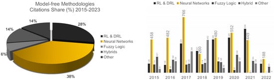
Figure 1.
The Model-free HVAC control citations share (%) per methodology (left) and the HVAC citations count per methodology (right) for the 2015–2023 period.
One particular segment of the model-free control considers the mathematical framework of ANNs. Inspired by the human brain’s processing capabilities, it has the potential to be trained, to learn from data, and to adapt over time. Unlike many traditional and intelligent methodologies, ANNs do not require explicit programming or extensive system knowledge [44,45,46]. Leveraging their capability to identify patterns, such mathematical frameworks become exceptionally proficient at predicting energy system behaviors in dynamic environments such as buildings. According to the literature [47], ANNs have shown a remarkable ability in handling non-linearities, uncertainties, and multi-variable systems, often outperforming other techniques in terms of accuracy and adaptability. Their capacity to integrate vast amounts of data, from various sensors and sources, and to derive actionable insights sets them apart [48,49,50]. The potential of ANNs in BEMSs has been further enhanced with the introduction of deeper neural network architectures that consider large-scale mathematical structures that are able to capture complex relationships and patterns in vast amounts of building data [51,52,53]. Such frameworks allow for even more accurate insights into building dynamics, from occupant behavior to equipment inter-dependencies. This evolution in control strategy, driven by deep learning, heralds a new era for BEMSs, where energy savings and comfort are optimized and adapted to both external factors and internal demands [49]. Figure 1 illustrates the importance of an ANN-based control as a mandatory model-free approach for HVAC systems (2015–2023), which portrays the most common BEMSs in building structures [34]. At this point, it should be noted that deep learning principles may extend beyond traditional artificial neural networks (ANNs), such as through incorporating elements from other machine learning methods such as regression, random forests, and SVMs.
Yet, as with any technology, ANNs are not without their challenges as training them requires a considerable amount of data, and ensuring their robustness and reliability in real-world scenarios remains a pressing concern. Moreover, their black box nature may raise concerns, particularly in critical systems where understanding the rationale behind decisions is crucial [49,51].
Motivated by the extended use of ANNs for predicting and optimizing energy system behavior in buildings in a building environment, the current work evaluates several highly cited ANN-based works from 2015–2023, and it considers the optimization of different BEMSs, such as HVAC, DHW, LS, and RES frameworks, along with their integrated applications. By analyzing different ANN methodologies and concepts, the primary aim of the current work is to gather, categorize, and evaluate their different attributes, as well as to consider the aggregated studies and to provide a thorough evaluation of the different patterns and trends that the ANN control frameworks exhibit toward BEMSs. Identifying such patterns is essential for identifying future directions, to obtain meaningful conclusions regarding the capacity and potential of ANN-driven applications in BEMSs, and to deliver a comprehensive overview of the particular control domain.
1.2. Paper Structure
This paper is structured as follows: In Section 1, the motivation of this work is assessed along with the literature analysis scheme that was adopted. In addition, prior related works in the literature are also considered, as well as the novelties and contributions of the current effort. In Section 2, the general framework of BEMSs is assessed, the operation of the different equipment of the BEMSs at the building level are described. Section 3 illustrates the mathematical background of the following different ANN architectures for the BEMS control under different BEMSs: feedforward neural networks (FNNs) and recurrent neural networks (RNNs). Section 4 includes the primary literature review of the integrated papers per ANN type, where each concept and approach is analyzed along with their particular outcome. Also, the tables include the common features of the integrated works that are generated and summarized in order to help the reader identify a general overview of the 2015–2023 studies. Section 5 includes an evaluation section, which is grounded in the examination of numerous impactful works of 2015–2023 in an effort to identify the different trends, trajectories, and concepts in ANN-based control toward BEMSs. Numerous diagram-based comparisons were conducted between the different concepts in order to identify the forthcoming tendencies in the field. To this end, Section 6 identifies the current trends and future directions in the field of ANN applications for BEMSs. Last but not least, Section 7 summarizes the overall conclusions of the current research effort.
The aforementioned seven sections illustrate the structure of the paper, and they may be described by the following Figure 2.
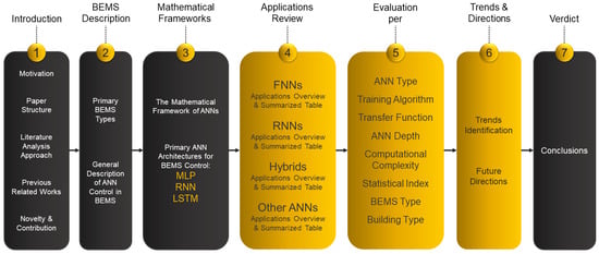
Figure 2.
The paper structure.
1.3. Literature Analysis Approach
In this comprehensive review, the primary objective was to explore, in depth, the impactful publications on ANN-based controls for different energy management systems at the building level (BEMSs), thus generating fruitful trends and conclusions, as well as determining the future directions in the field. To this end, the study dives deep into a broad range of studies, inspecting their core concepts, management techniques, utilized algorithms, and distinct implementations. Moreover, by illustrating the different fields of ANN-based control into different sub-divisions depending on the ANN type, training methodology, individual model characteristics, as well as the type of BEMS and the building testbed characteristics, this study provides a holistic overview of the field to the potential user. Our procedure is systematic, and it guarantees that each chosen study is meticulously analyzed.
- Article Criteria: The integrated studies were selected based on the subsequent themes: ANNs for building management; ANNs for HVAC management in buildings; ANNs for hot water management in buildings; ANNs for lighting management in buildings; ANNs for renewable energy management in buildings; and ANNs for storage management in buildings;
- Keyword Selection: The appropriate keywords linked to our topic were explored in contemporary studies. The search strings encompassed the following: predicting BEMS behavior via ANNs; predicting HVAC behavior via ANNs; predicting domestic hot water via ANNs; predicting building lighting via ANNs; and predicting building renewable energy via ANNs. These phrases were selected as they recognize the distinct challenges and aspects of predicting or optimizing the behavior of BEMSs.
- Article Selection: This particular research was grounded primarily on platforms like Scopus and Google Scholar, which directed the exploration of the numerous studies. After the preliminary overview of more than 200 papers via their summaries, the most pertinent ones were pinpointed for an in-depth examination.
- Data Collection: Subsequently, the data from each publication were classified, emphasizing the utilized ANN technique for BEMS management and the context of its use. Several aspects were taken into account, such as advantages, constraints, and real-world implications, especially in relation to optimal BEMS management scenarios.
- Quality Assessment: Every chosen study underwent a validity evaluation based on multiple standards. These standards involved the paper’s citation count, the academic input of the contributors, and the research techniques utilized. This helped in determining the relative significance and influence of each study.
- Data Analysis: In conclusion, the collected insights were arranged into distinct groups, thus facilitating straightforward comparison and comprehension.
1.4. Previous Literature Work
In the literature, numerous reviews regarding ANNs toward BEMSs have been conducted. In [54], Georgiou et al. illustrated the core principles of ANNs and explored their diverse applications in the realm of building operations, including energy efficiency, system regulation, and forecasting energy usage. Such work revealed that the employment of ANNs in building environments may potentially lead to notable decreases in energy use—though this varied with the application. Additionally, the review underscored the significant promise of ANNs for advancing effective control strategies and energy reduction in the broader energy and construction industries. In [55], Runge et al. presented an analysis of the research conducted since 2000, and they focused on the use of ANNs in predicting energy usage and demand in buildings. Their work was focused on examining the various applications, datasets, predictive models, and evaluation criteria employed in the studies analyzed. Moreover, in [56], Mohandes et al. illustrated numerous key studies that utilized ANNs in building energy analysis (BEA). Such work covered the extensive research on ANNs applied to energy issues in buildings, focusing on areas like water heating and cooling systems, the prediction of heating and cooling loads, heating ventilation air conditioning system modeling, indoor air temperature forecasting, and building energy consumption estimations. Last but not least, in [57], Guyot et al. introduced an in-depth analysis of the research utilizing neural networks for energy-related applications in buildings, and they emphasized their deployment and technical aspects such as learning algorithms, network layers, neuron count, input/output variables, and performance metrics. Their review identified the limitations and research gaps in the use of neural networks in the building sector, as well as suggested potential avenues for future investigation.
1.5. Novelties and Contributions
The current work stands out in the landscape of the existing literature by offering an unprecedented synthesis of the most influential research from 2015 to 2023. This work delves into the framework of ANN methodologies and their applications within BEMSs, casting a wide net to capture a holistic picture of the field. The current effort analyzes the domain into distinct categories, examining ANN techniques as they specifically apply to different BEMSs, such as HVAC equipment, DHW systems, LSs, and RESs in buildings. Each category is thoroughly analyzed through the prism of the unique features and challenges of the respective test bed cases, with a sharp focus on the delicate differences between them.
Contrary to the majority of the aforementioned works, the current effort illustrates, in detail, the concept of each integrated work, highlighting the ANN model architectures and individual characteristics along with the outcomes of each research. Then, different important fields were evaluated, such as the different data elements that were utilized for training the models (5.1), the prevalence per ANN type (5.2), training scheme prevalence (5.3), utilized transfer functions (5.4), the depth of the ANNs (5.5), the computational complexity of the ANNs (5.6), as well as the utilized statistical indices (5.7). Last but not least, this work also focused on the test bed characteristics by evaluating the prevalence of each BEMS type (5.8) and the features of the building test bed (5.9). The following Table 1 provides a comparison of the evaluation that previous works and the current review conducted.

Table 1.
Comparisons of the current work with previous works.
It should be also mentioned that the current research effort does not just stack research side by side but quantifies their impact by citation share, illustrating the relative influence and traction each segment has gained in the research community. To this end, this study provides an in-depth comparative analysis between the different ANN architectures, and it draws conclusions that are both meaningful and well founded on robust comparative frameworks. Consequently, the trends and future directions in the field are established, and insightful directions for forthcoming research are provided. By navigating through the complexities of ANN-based control and modeling—and their efficacy in different BEMS applications—the current effort lays out a path forward for the field, highlighting emerging trends and potential paradigm shifts that could redefine building energy management.
2. Building Management Systems and Operation
2.1. Primary BEMS Types
BEMSs are crucial for the automation and optimization of energy use within a building’s various systems. ANNs play a pivotal role in such devices by enabling the predictive control and optimization of energy usage. They analyze historical and real-time data to forecast energy demand, enhancing the efficiency of heating, cooling, and lighting equipment. ANNs also adapt to changing environmental conditions and user behaviors, ensuring optimal energy consumption while maintaining the comfort levels in buildings. The following attributes break down the operation of the most common BEMSs and illustrate their challenges regarding the relative ANN applications [7,58]:
- Heating, Ventilation, and Air Conditioning (HVAC): HVAC systems regulate the indoor climate to maintain comfort. They are complex with fluctuating loads and numerous sub-components, thus making them prime candidates for ANN-based optimization. The challenge lies in creating sufficient ANN models to accurately predict thermal loads and system responses to various conditions. ANNs need extensive training data to capture all possible scenarios, including seasonal changes and occupancy patterns.
- Domestic Hot Water (DHW): DHW systems provide hot water for residential or commercial use. ANN-based controls for DHW systems may predict hot water demand and optimize energy use while ensuring availability. The challenge is to model the sporadic usage patterns and integrate them with other systems like solar heating, which can be unpredictable due to weather variations.
- Lighting Systems (LSs): Smart lighting controls adjust based on occupancy and ambient light levels. ANN can optimize lighting for energy savings while maintaining comfort. The challenges include the need for real-time responsiveness to sudden environmental changes and accurately modeling human presence and movement patterns.
- Renewable Energy Systems (RESs): These include photovoltaic panels, wind turbines, etc., which supply sustainable energy. ANN-based controls are adequate for predicting energy production and managing storage or grid exports. Challenges arise from the inherent unpredictability of renewable sources and the complexity of integrating them with traditional energy systems. (It should be mentioned that, while RESs like wind and solar power are inherently variable, advancements in weather forecasting and predictive analytics have greatly improved their predictability. This technological progress enables more reliable energy production forecasts, thereby mitigating the impact of their natural unpredictability. Thus, the integration and stability of renewable energy in power systems are continuously enhancing).
- Energy Storage Systems: Batteries and thermal storage systems are used to balance supply and demand. ANNs may provide predictions of when to store energy and when to release it based on predictions of future energy prices and demand. The main challenge is the dynamic nature of energy markets and consumption patterns.
- Integrated Building Management Systems (IBEMSs): IBEMSs concern the integration of multi-device systems, including the abovementioned BEMSs, or any other appliances in the building environment, for holistic building energy management.
The multiverse role of ANNs with respect to the different BEMSs are summarized in the following Figure 3.
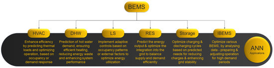
Figure 3.
The role of ANN applications for BEMS control and optimization.
2.2. General Description of ANN-Based Control in BEMSs
In order to provide the abovementioned functionalities for the different BEMSs, ANNs may be utilized in a specific manner. To this end, the general operation of ANNs in controlling the different BEMS frameworks typically follows a process of data collection, model training, prediction, and control action. The following Figure 4 provides a diagrammatic representation of the process:
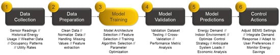
Figure 4.
The general scheme of ANN-based control for building management systems (BEMSs).
More specifically, the five-step methodology of Figure 4 integrates the following aspects:
- Data Collection: This involves gathering BEMS-related real-time data from environmental sensors, energy meters, and other IoT devices, along with historical energy usage patterns, current weather conditions, occupancy levels, equipment status, and utility rates. These data form the basis for making informed decisions.
- Data Preparation: The raw data undergo rigorous cleaning to rectify inconsistencies and fill gaps, and this is followed by feature engineering to highlight relevant predictive factors. This process is crucial for fostering the ANN’s predictive accuracy, thus ensuring it receives quality input for optimal energy management performance.
- Model Training: In this step, the ANN is configured and trained using historical data, weather forecasts, and feature selection to recognize patterns and dependencies. The ANN architecture is designed and the parameters are optimized.
- Model Validation: In this stage, a dedicated validation dataset is utilized to evaluate the model’s predictions, while cross-validation ensures the model’s performance is consistent across different subsets of the data. A performance metric analysis is conducted assessing accuracy, precision, and other relevant metrics to gauge the model’s predictive power.
- Model Predictions: The trained model is then used to forecast future energy demand, predict indoor environmental conditions, and perform optimization with the help of the model predictive control. This includes determining the best start and stop times for equipment, anticipating system loads, and conducting economic analysis for cost-saving measures.
- Control Actions: The final step is where the BEMS acts on the ANN and outputs to the control the building’s energy systems. This includes adjusting HVAC settings, regulating lighting, operating shades and blinds, managing RES, integrating demand response strategies, adapting to user preferences, and monitoring/reporting on energy savings to stakeholders.
3. Conceptual Background of the Neural Network Architectures for BEMS Control
Neural networks, at their core, are computational architectures/mathematical frameworks inspired by the neuronal structures of biological brains. These networks are composed of layers of interconnected nodes, often termed “neurons” (Figure 5—left). As Figure 5—right illustrates, each connection carries a weight and every neuron processes its input using an activation function to produce an output, thereby determining the strength and influence of the transferred information. Additionally, each neuron possesses a bias (Figure 5—right), a unique baseline from which it operates, thus ensuring that, even in the absence of any input, it holds influence. This layered and interconnected structure enables neural networks to model/express intricate and non-linear relationships within data. For a potential building management system, the predictive process of ANNs is most commonly tailored to optimize energy usage and efficiency. The network starts by receiving diverse input data, such as temperature, occupancy, energy consumption patterns, weather forecasts, and time of day. As this data traverses through the network’s layers, each layer performs specialized transformations, extracting key features relevant to energy management. The flow of the data from node to node is governed by activation functions. Such functions introduce the necessary non-linearities, enabling the neural network model to capture the intricate relationships in the data they process, and they thus provide predictions aligned with the behavior of a potential BEMS framework.
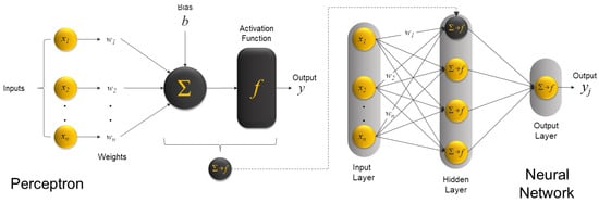
Figure 5.
From a single perceptron to an ANN.
Training a neural network involves iteratively adjusting its internal parameters, primarily the weights and biases associated with each neuron, to better fit a given dataset. This adjustment process typically uses optimization algorithms, with gradient descent being among the most prevalent. The process begins with a forward pass of data, resulting in a prediction. This prediction is then compared with the actual behavior of a potential BEMS framework, which thus produces an error. Algorithms—such as the well-known gradient descent—are commonly used to back-propagate this error, analyze it, and delicately adjust the weights and biases throughout the network using techniques like the chain rule of calculus. In using multiple iterations, over multiple passes—or epochs—through the training data, the network fine tunes its parameters to approximate the underlying function of the data it is exposed to. Over time, as the network is exposed to more data and feedback, it fine tunes its predictions, leading to a more intelligent and efficient energy management system.
Beyond these internal parameters, neural networks also include hyperparameters, which are not learned from the training process but are set beforehand. These include choices such as the number of layers in the network, the number of neurons in each layer, the type of activation function, and the parameters related to the optimization process like the learning rate. The proper selection of hyperparameters is crucial and portrays an interesting topic in research as they can significantly influence the performance, training speed, and generalization capability of the network.
3.1. The General Concept of ANNs for BEMS Control
To this end, before its utilization as a BEMS prediction tool, the neural network is trained on historical data and applies learned weights and biases to these inputs, refining them at each step. This continuous refinement helps the ANN framework to be aligned toward complex relationships and patterns in the data, such as how weather impacts energy use or the correlation between occupancy and heating needs. In the final stage, the output layer synthesizes these insights into predictions or decisions, such as adjusting thermostat settings, optimizing lighting, or scheduling maintenance activities for energy systems. The network’s predictions are most commonly geared toward reducing energy consumption while maintaining comfort and efficiency, thus aligning with the primary goals of a BEMS. As already mentioned, the neural networks are composed of layers of interconnected nodes (or the so-called neurons).
To properly describe the operation of an ANN, we can detail the simplest form of an ANN, which can be described by a perceptron. Introduced in 1957, a perceptron consists of input nodes (or units), weights, a bias, and an activation function. It is primarily used for binary classification tasks, and it serves as a foundational concept for understanding more complex neural network architectures. The perceptron concept is described in Figure 5—left. The formula for directly expressing the output y of a perceptron, including the bias term, is as follows:
where is the weighted sum of the inputs; is the weights; is the input values; b is the bias term, which is added to the weighted sum; and f is the activation function applied to the sum of the weighted inputs and the bias. It should be noted that, for the simple perceptron, this is typically a step function as follows:
where y takes the value of 1 if the weighted sum plus the bias is non-negative, or it is 0 otherwise. This binary output is what makes the perceptron suitable for binary classification tasks.
The real strength of ANNs is unveiled when multiple perceptrons are stacked in layers to overcome the limitation of linear decision boundaries, which a single perceptron integrates. (Figure 5—right). Such networks are adequate for a modeling the complex, non-linear relationships in data. The training process for ANNs involves adjusting the weights and biases of all neurons (including perceptrons in the network) based on the network’s performance on training data. Such a form of a neural network consists of an input layer, one or more hidden layers, and an output layer, as illustrated. The operation may be described as follows:
- Input Layer: Receives raw input data that are analogous to the external stimuli in biological systems.
- Hidden Layers: Process the inputs via weights adjusted during training. The neurons in these layers apply activation functions to the weighted inputs and relay the result to the next layer.
- Output Layer: Produces the final result or prediction.
Similarly, the mathematical representation of the general neural network concept may be described as follows:
Neuron Computation: As already mentioned, the basic computational unit of an ANN is the neuron. Each neuron receives inputs, processes them, and produces an output. The output of the neuron is computed as follows:
where f is the activation function; represents the weight connecting the input to the neuron; is the input to the neuron; is the bias term for the neuron; and n is the number of inputs.
Activation Functions: Activation functions introduce non-linearities into the network, thereby allowing it to model complex, non-linear relationships. Some common activation functions include the following:
- Sigmoid: Sigmoid is an activation function that maps any input value to a value between 0 and 1. It is commonly used for models where the output represents a probability, such as in binary classification problems. (sig): ;
- Hyperbolic Tangent: Tanh is a mathematical function used in neural networks as an activation function. It outputs values between −1 and 1, making it effective in handling negative inputs. (tanh): ;
- Rectified Linear Unit: ReLU is a popular activation function in neural networks, particularly in deep learning models. It outputs the input directly if it is positive, and if it is such, it outputs zero.
- It offers efficient computation and mitigating the vanishing gradient problem (ReLU): ,
where z concerns the pre-activation value computed from the inputs to a neuron, which it serves as the input to the activation function, thus determining the neuron’s output based on the non-linear transformation applied by the activation function. Meanwhile, represents the output of the activation function for that given input z.
Training Algorithm: The most common training algorithm for ANNs is backpropagation. The goal is to minimize the difference between the network’s output and the desired output for a given set of inputs. The process involves the following: (1) performing a forward pass to compute the network’s output; (2) calculating the error between the network’s output and the desired output; and (3) propagating this error backward through the network to update the weights and biases. The weights are updated most commonly using the gradient descent method:
where is the learning rate and E is the error function, which is commonly the mean squared error for regression problems. This process is repeated for multiple iterations or epochs until the network converges to an optimal solution.
3.2. Primary Artificial Neural Network (ANN) Architectures for Building Energy Management Systems (BEMS) Control
Common architectures concerning BEMSs consider, most commonly, FNNs—especially the multilayer perceptron (MLP)—while the presence of RNNs is evident in numerous applications. A specialized RNN type—the long short-term memory network (LSTM)—concerns the most common type of RNNs utilized in the literature, which are particularly effective toward sequences and time series data.
3.2.1. Feedforward Neural Networks
FNNs portray the foundational type of neural networks with a linear architecture, where data flow unidirectionally from the input to output layers without any cycles or loops. They consist of multiple layers of neurons, each layer fully connected to the next, and they are typically used for tasks like classification. FNNs excel in learning mappings from inputs to outputs, making them versatile for a wide range of applications. FNNs concern the most common generalized architecture for controlling BEMSs in the literature due to numerous reasons:
- Simplicity and Efficiency: FNNs offer a straightforward architecture, making them relatively easier to implement and train compared to recurrent or more complex networks.
- Capability to Capture Non-linearities: BEMS systems, especially components like HVAC, water heating, and lighting, exhibit non-linear behaviors. FNNs can model these non-linear relationships effectively, making them ideal for such applications.
- Scalability: FNNs can be scaled with multiple hidden layers and neurons to handle the complexity introduced by integrating RES and storage systems in BEMSs.
It should be noted that, while simple FNNs—which have a single layer—are potentially adequate for approximating linear relationships, the interactions within BEMSs are inherently non-linear and multi-faceted given the myriad of subsystems like HVAC, lighting, and water heating operating in tandem. This is where MLPs come to the fore: MLPs concern a type of FNN with one input layer, one or more hidden layers, and one output layer. Each layer is fully connected to the subsequent layer. By integrating multiple layers of neurons, MLPs introduce additional depths of transformation to the data, allowing them to capture and represent more complex and non-linear relationships. The MLP conceptual background may described as follows: for a given input vector X, the output from the first hidden layer is
where is the weight matrix connecting the input layer to the first hidden layer and is the bias vector for the first hidden layer. For subsequent layers, the output is computed similarly, using the output of the previous layer as the input. For example, the output from the second hidden layer is as follows:
and so forth, until the final output layer. Each additional layer in an MLP can be viewed as enabling the network to learn hierarchical features, where initial layers capture basic patterns and subsequent layers build upon them to understand more intricate relationships. This hierarchical learning capability ensures that MLPs are adequate for modeling the nuanced behaviors and interactions in BEMSs with a higher degree of accuracy.
Furthermore, the depth provided by multiple layers in MLPs allows for a richer set of weights and biases, thereby offering more degrees of freedom during training. This results in a more flexible model that can better adapt to the complexities of BEMS data. In essence, while simpler FNNs might suffice for rudimentary tasks, the multifaceted challenges posed by BEMS control and modeling necessitate the enhanced capabilities and depth offered by MLPs. A typical FNN (MLP) is illustrated in Figure 6—left, whereby four nodes are integrated in the input layer, three nodes in the first hidden layer, four nodes in the second hidden layer, and two nodes in the output layer.
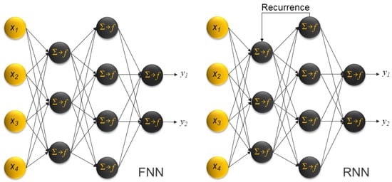
Figure 6.
Primary ANN architectures utilized for BEMS applications: feedforward neural networks and recurrent neural networks.
3.2.2. Recurrent Neural Networks
RNNs portray a type of neural network suitable for processing sequential data, where the output from previous steps is fed back into the network as the input for the current step. This looped architecture enables RNNs to maintain a form of ’memory’, making them ideal for tasks involving time series data. RNNs are distinguished by their ability to capture temporal dynamics and contextual information in sequences, which is not possible with traditional FNNs. To achieve this objective, RNNs take into account the time-related changes in Building Energy Management System (BEMS) control. This approach enables previous circumstances and activities to impact current control choices, rendering them highly suitable for forecasting extended environmental alterations. A typical RNN is illustrated in Figure 6—right, where four nodes are integrated into the input layer, three nodes in the first hidden layer, four nodes in the second hidden layer, and two nodes in the output layer.
Given an RNN, the basic operation can be described as follows:
- Hidden State Update:where is the hidden state at time t; is the hidden state at the previous time step; is the input data at time t; is the weight matrix for the hidden state; is the weight matrix for the input; is the bias for the hidden state; and is the activation function.
- Output:where is the output at time t; is the current hidden state; is the weight matrix for the output; and is the bias for the output. Training an RNN involves adjusting the weights and biases (, , , , and ) using historical data to minimize the prediction error.
As MLPs, RNNs also hold specific advantages:
- Memory Capability: The intrinsic ability of RNNs to remember past inputs makes them exceptionally suitable for systems with temporal dependencies, like the energy consumption patterns in BEMSs.
- Handling Sequence Data: BEMSs often deal with time series data, such as the hourly energy consumption or daily temperature variations. RNNs are naturally suited to process and predict based on such data.
3.2.3. Long Short-Term Memory Networks
In the context of BEMS control and modeling, LSTMs offer a distinct advantage over traditional RNNs. BEMSs often deal with time series data that contain long-term dependencies, such as seasonal patterns or latent factors from historical data. Conventional RNNs, while designed to handle sequences, struggle with such long-term dependencies due to the vanishing gradient problem, thus leading to difficulties in retaining information from earlier time steps. LSTMs, on the other hand, are specifically engineered to combat this issue. With their unique architecture comprising forget, input, and output gates, LSTMs can selectively remember or forget information, making them adept at capturing and modeling long-term patterns in BEMS data. This ability ensures more accurate predictions and robust control strategies, making LSTMs a preferred choice for complex BEMS applications where understanding temporal dependencies is crucial. Given the foundational structure of an RNN, LSTM extends its capabilities with specialized gates to better handle long-term dependencies. The primary operations in an LSTM are as follows:
- Forget Gate:
- Input Gate:
- Update of the Cell State:
- Output Gate:
where concern the forget, input, and output gates, respectively, at time t; portrays the candidate cell state at time t; portrays the cell state at time t; portrays the hidden state at the previous time step; portrays the input data at time t; concern the weight matrices for the forget gate, input gate, candidate cell state, and output gate, respectively; concern the biases for the forget gate, input gate, candidate cell state, and output gate, respectively; portrays the sigmoid activation function; and tanh portrays the hyperbolic tangent activation function.
Within the realm of BEMS control and modeling, LSTMs have emerged as a superior choice over traditional RNNs. One of the key challenges with RNNs is the vanishing gradient problem, where the gradients of the loss function become too small for effective learning, thus causing the network to forget long-term dependencies. Conversely, RNNs may also suffer from the exploding gradient problem, where the gradients become excessively large, thereby leading to unstable training. LSTMs, with their intricate gate mechanisms—comprising forget, input, and output gates—are ingeniously designed to mitigate both of these issues.
4. Literature Review of Neural Network Applications for BEMS Control
This section exhibits numerous highly cited ANN research applications related to BEMS control and optimization in order to discriminate them into the aforementioned ANN types: FNNs; RNNs; hybrid control applications—which concern the integration of ANNs with each other or with other methodologies; and other ANN applications that do not concern any of the aforementioned types. To this end, the current section explores the integrated research applications, in which their underlying motivations and the conceptual methodologies of ANNs used are thoroughly detailed. It elaborates on the structure of each potential ANN, encompassing a comprehensive characterization of inputs, outputs, hidden layers, and the overall architecture of the models. Additionally, the outcomes of these applications are thoroughly analyzed in terms of statistical measures.
In the final part of each sub-section, the tables conclude by providing additional summarized information on the related highly cited research works of 2015–2023. To this end, Table 2, Table 3, Table 4 and Table 5 contain the following features toward each ANN application:
Table 2.
Summarized FNN approaches for BEMS control (2015–2023).
Table 3.
Summarized RNN approaches for BEMS control (2015–2023).
Table 4.
Summarized hybrid approaches for BEMS control (2015–2023).
Table 5.
Summarized other approaches for BEMS control (2015–2023).
- Reference: Denoted as Ref. in the first column;
- Year: Illustrates the publication year of each research application;
- ANN Type: Illustrates the specific ANN type utilized in each work;
- Training Scheme: This attribute concerns two elements. The first defines which algorithm was utilized for training the particular ANN model (e.g., GD—gradient descent), while the second (which is separated by “/”) defines the optimization methodology (e.g., BP—backpropagation) that was utilized;
- Transfer Function: Denotes which transfer function(s) were integrated into the nodes of the ANN model;
- Hidden Layers: Defines the number of hidden layers of the selected ANN model, as denoted in the literature;
- BEMS Type: Illustrates the specific BEMS type that concerns each of the following applications as denoted in the published work—heating, ventilation, and air-conditioning are denoted as HVAC; water heating and DHW applications are donated as DHW; lighting systems are denoted as LSs; renewable energy source-related applications are denoted as RES;
- Residential: Defines whether the testbed application concerns a residential building control application with an “x”;
- Commercial: Define whether the testbed application concerns a commercial building control application with an “x”;
- Citations: Last but not least, the citation count of each work is illustrated according to Scopus.
The abbreviation “N/A” or “-” represents the “not identified” elements in the Tables and Figures.
4.1. Review of the FeedForward Neural Network Applications for BEMS Control
In a 2015 study, Afram et al. [59] focused on developing and comparing models for various HVAC subsystems, such as the energy recovery ventilator (ERV model structure—4:10:2), air handling unit (AHU model structure—1:10:1), buffer tank (BT model structure 8:10:1), radiant floor heating (RFH model structure—1:10:2), and ground-source heat pump (GSHP model structure 2:10:1). The hidden layers for each ANN model structure was defined at 10 nodes, while sigmoid was elected as the activation function for each node of the models. Except from the FNNs, the different model types were thoroughly examined—including the transfer function (TF), process, state-space (SS), and autoregressive exogenous (ARX) types—and this was achieved using system identification techniques in MATLAB. The study also contrasted these newly created black box models with previously established gray box models. After evaluating the models in the visual and analytical mode, FNNs emerged as the top performer, followed by the ARX, TF, SS, process, and gray box models in descending order of performance.
The same year, Zhang et al. [60] examined the efficiency of the data-driven models in predicting HVAC hot-water energy consumption in office buildings. Four models—change-point regression, Gaussian process regression, Gaussian mixture regression, and ANN—were evaluated using pre-retrofit building data as the baseline for retrofit projects. Each model’s performance was gauged using metrics such as , RMSE, and . The model structure accounted for the dry bulb temperature, solar radiation, humidity, as well as other variables as inputs to a FNN architecture with two hidden layers, where each layer is composed of 20 neurons and features a single-output neuron (which was aligned with the target value). According to the evaluation, the Gaussian mixture regression model slightly outperformed the others, while the FNN model required more training data. Despite their differences, all models, barring FNN, aligned with the ASHRAE Guideline 14 criteria for hourly predictions.
Also in 2015, Ardabili et al. [61], aimed to enhance the control accuracy of an HVAC system by employing both a fuzzy control system and a radial basis function (RBF) model—a specific type of FNN—for predictive management. The model was developed to utilize temperature and humidity as inputs to predict the following four output variables: the coil valve, circulation air damper, fresh air damper, and moisture pump valve. The single hidden layer nodes varied from 4 to 24, where 20 was determined as the optimal value. According to the evaluation, the RBF network consistently outperformed the fuzzy system across all metrics. More specifically, the RBF network exhibited lower values for MAE (0.045908 for temperature and 0.054455 for relative humidity), MAPE (0.002181 for temperature and 0.000605 for relative humidity), and RMSE (0.0699 for temperature and 0.0903 for relative humidity). In addition, the RBF network showcased a high correlation coefficient (0.9243 for temperature and 0.8522 for relative humidity), thus indicating a strong linear relationship between its predicted and actual values, as well as highlighting its superior learning capability.
In 2016, a novel research conducted by Idowu et al. [62] presented a comprehensive examination and forecast of heat load in buildings, which included aspects of both the building space and DHW. This was achieved through the following various machine learning (ML) methodologies: support vector machine (SVM), FNN, multiple linear regression (MLR), and regression tree. The information for constructing these models was derived from ten buildings, which were split evenly between residential and commercial types, located in Skellefteå, Sweden. The prediction models utilized inputs such as external temperature, historical heat load data, time-based variables, and the details of the district heating substations. The FNN algorithm was employed with N hidden layers, with the ideal N being chosen for each building’s dataset. The models’ performances were evaluated over forecast intervals that spanned from 1 to 48 h. The results revealed that SVM, FNN, and MLR were more effective than the regression tree method, and that they demonstrated comparable prediction accuracy while incorporating fewer errors in their forecasts.
The same year, Renno et al. [63] developed and evaluated two FNN models to accurately predict solar radiation metrics: (a) daily global radiation (GR) and (b) hourly direct normal irradiance (DNI). By exploiting a mix of climatic, astronomic, and radiometric data, the models’ performances were evaluated under different neural network configurations, and the best ones were further assessed on new datasets. In both FNN models, the hidden neuron number started at 8 and increased until performance declined at 12 neurons, thus indicating 10 as the optimal number. Moreover, different combinations of activation functions were evaluated, indicating the tanh–tanh–lin configuration as the most appropriate one for both models. The results indicated correlations with the MLP models, which were then used to estimate the electrical energy output of the two different photovoltaic systems for a residential building. According to the evaluation, the GR model achieved a MAPE of 4.57%, an RMSE of 160.3 Wh/m2, and an of 0.9918, whereas the DNI model obtained a MAPE of , an RMSE of 17.7 W/m2, and an of 0.994.
In 2017, Ahmad et al. [64] conducted a study that assessed the effectiveness of a standard FNN trained with backpropagation in predicting the hourly HVAC energy use of a hotel in Madrid in comparison to a random forest (RF) model—another method that is gaining popularity in forecasting. Incorporating factors like the guest count slightly improved the predictions for both methods. When evaluating based on criteria such as the root–mean–square error (RMSE), the mean absolute percentage error (MAPE), the mean absolute deviation (MAD), the coefficient of variation (CV), and the metrics, the FNN surpassed the RF model in all measurements. Though it should be underlined that both methods showed nearly identical accuracy, thereby indicating that they were both suitable for building energy predictions. The structure of the MPL involved a single hidden layer with 10–15 neurons featuring a single output neuron, which was aligned with the target value. The quantity of the input nodes varied, including a range chosen from ten factors like the outside air temperature, dew point temperature, relative humidity, wind velocity, hour of the day, day of the week, month of the year, daily guest count, and the total number of rooms reserved.
Also in 2017, Park et al. [65] investigated the performance of a ground-source heat pump system (GSHP) that supplied heating and cooling to a hospital (Figure 7). The GSHP system’s seasonal heating efficiency and operational characteristics were analyzed using real-time data. The researchers then developed two prediction models for the system’s performance: one based on multiple linear regression (MLR) and the other on an FNN. After an exploratory data analysis (EDA) on the raw data, the final FNN model featured 13 input variables and 3 hidden layers with 10, 5, and 2 neurons each. The MLR model was further refined to study the impact of specific variables, such as the temperatures of the source and load water inputs. When comparing the accuracy of the two models, the FNN model proved to be more precise than the MLR model. According to the evaluation (which was based on the coefficient of variation of the RMSE with no significant bias), when comparing the prediction accuracy, the MLR method exhibited a deviation of 3.56%, while FNN showed a tighter accuracy with a deviation of 1.75%.
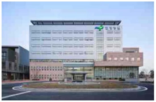
Figure 7.
Park et al. [65] use case: University Hospital, Republic of Korea.
In an interesting study in 2018, Kandasamy et al. [66] introduced an innovative lighting control solution for net-zero energy buildings (NZEBs). The system was modeled using an FNN architecture integrated with the internal model control (IMC) principle for controller creation. Using FNN for modeling the lighting system simplified the task, thereby removing the need to handle vast and intricate systems and extensive data analysis. The suggested ANN-IMC controller relied on sensor feedback to maintain the desired light levels, and it is both easy to adjust and robust against variability. The training data for both modes, derived from testbed experiments (Figure 8), comprised illuminance levels (lux) in tables and light power settings ranging from 0 to 100% in 5% increments. The single hidden layer for both models consisted of 10 neurons, thus reducing the overall data required for modeling. The outcome indicated energy savings of 54% and 40% regarding the desired light intensities of 300 lux and 500 lux, respectively, when compared to the baseline control approach.
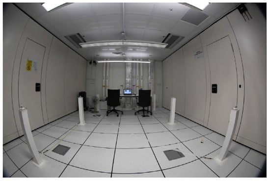
Figure 8.
Kandasamy et al. [66] use case: SinBerBest Laboratory, National University of Singapore.
The same year, Markovic et al. [67] focused on the importance of accounting for occupant behavior, specifically window openings, in building performance simulations, which were used to estimate indoor climate and energy usage for HVAC systems more accurately. Traditional models often integrate biases and inefficiencies to handle large numbers of occupants. To address this, a Deep FNN model has been introduced in the current research for the purpose of predicting window openings in commercial buildings. The model was trained using data from a German office, and it was then tested on three distinct buildings. The network integrated an input layer of 25 neurons: 22 for the current time step features, and 3 for the indoor temperature, humidity, and CO2 from 10 min earlier (while the output layer contained one neuron for window state prediction). The model’s practicality was evaluated by integrating it into a Modelica-based building thermal simulation, which presented accuracy rates between 86–89%, with the (F-score statistical measure) ranging from 0.53 to 0.65 across the office buildings. Notably, while the model’s performance saw a decline of around 15% with limited input data, the score remained relatively high.
Also in 2018, Gonzales et al. [68] presented a new multi-agent system (MAS) in a cloud setting. This system, combined with a wireless sensor network (WSN), aimed to improve HVAC energy efficiency. The agents in the MAS learned from data and used a neural network (ANN) to understand the patterns. The system used sensor data to adjust to building conditions and the number of people present. It also considered the weather predictions and times when the building (Figure 9) was not in use to fine tune the HVAC system’s operation. The FNN employed a sigmoidal activation function to prevent extreme values during training with the hidden layer containing neurons, where n equals the number of input neurons. This method allowed for steadier temperature changes, thus avoiding sudden jumps that increased energy use. Their tests showed that this approach saved an average of 41% of energy in office environments. Interestingly, the energy saved was not always directly tied to the difference in the indoor and outdoor temperatures.
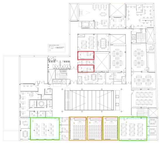
Figure 9.
Gonzales et al. [68] use case: seven offices, University of Salamanca, Spain.
Deb et al. [69] in 2018, established two predictive tools to save energy in HVAC systems for commercial buildings located in Singapore. By exploring both multiple linear regression (MLR) and ANN models such as MLPs, the primary aim of the work was to efficiently compare the aforementioned approaches and identify the best potential prediction model. To this end, 1 to 14 input variables from pre-retrofit energy audit reports were tested to identify the optimal MLP structure for predicting changes in the energy use intensity (EUI). The number of neurons in the hidden layer was fixed at 4, and this was determined through a sensitivity analysis involving 2–8 neurons. The outcome showed that the MLP illustrated an improved prediction performance of about 14.8% in the EUI in comparison with the MLR methodology.
In a 2019 study, Peng et al. [70] introduced a learning-based control strategy aimed at allowing HVAC systems to adapt to individual thermal preferences as conditions change. The preference models were built using four key factors: time, indoor and outdoor weather conditions, and user behavior. A FNN, holding the best potential hyperparameters, was trained to predict the room temperature setpoint (Tsp) as adjusted by occupants. The structure of the model involved a two-layered MLP, in which the number of neurons in the hidden layer varied between 3 and 10. Over five months, this learning-based thermal preference control (LTPC) was tested on an HVAC system in both single-user and multi-user office settings. The results showcased energy savings between 4% and 25% compared to fixed temperature settings. Additionally, the need for manual temperature adjustment was significantly reduced from 4–9 days/month to just 1 day/month.
Also in 2019, Al-Waeli et al. [71] aimed to compare various photovoltaic thermal (PVT) integrated energy systems—including conventional PVT, water-based PVT, water-nanofluid PVT, and nanofluid/nano-PCM—under identical conditions. A single MLP was used for this evaluation. The study sought to understand the efficiency variations in these systems, both thermally and electrically, using a singular MLP simulation system. The input parameters of the model concerned two input nodes in addition to solar irradiation data, ambient temperature data, a single hidden layer, and a single output, where the voltage, current, electrical, and thermal efficiencies for each respective energy system were varied. The model exhibited an MSE of 0.0229 during training and 0.0282 during cross-validation. The results from the FNN model indicated that the nanofluid/nano-PCM system increased electrical efficiency from 8.07% to 13.32%, while its thermal efficiency reached 72%.
In the same year, Ren et al. [72] refined a sophisticated control model for HVAC systems to manage both indoor air quality (IAQ) and indoor thermal comfort (ITC) more effectively. The model utilizes low-dimensional linear models (LLVM for ventilation and LLTM for temperature) in conjunction with MLP neural networks and a contribution ratio index (CRI). The control system was underpinned by a database informed by computational fluid dynamics (CFD) and experimental data. The single-output ANN was specifically employed for IAQ prediction, where the air change per hour (ACH) and indoor pollutant sources were the inputs, and the indoor CO2 level was the output, thus aiding in expanding the CFD database for a more accurate control of the HVAC system. This integrated approach enabled rapid and accurate predictions of environmental conditions like the CO2 level and temperature. According to the evaluation, the application of this model in HVAC control can lead to significant energy savings, thereby reducing ventilation and air conditioning energy consumption by up to 50% and 32%, respectively.
In a 2020 study by Deng et al. [73], a new approach was introduced to improve HVAC systems in offices with multiple users by exploiting data from wearable wristbands to gather physiological information. Using an MLP, the model was adequate for predicting thermal feelings based on the following indoor conditions: air temperature, relative humidity (RH), clothing level, thermal sensation, wrist skin temperature, and wrist skin. The optimal structure of the model consisted of six neurons on the input layer feeding a single hidden layer, as well as six neurons featuring a single output neuron, which was aligned with the thermal sensation vote (TSV). The MLP model was trained for a year using data from seven different offices, and it demonstrated high prediction accuracy. Using this data, Deng et al. developed a control system for HVAC systems to adjust the thermostat in real-time, thus improving comfort. Testing through experiments and simulations showcased that over 50% of the users felt neutral in terms of the temperature, while only a minor percentage felt discomfort. The energy use was similar to standard systems, but when combined with controls based on occupancy—achieved using light sensors or Bluetooth from the wristbands—the heating and cooling needs dropped significantly by 90% and 30%, respectively, in certain office areas.
In another important study in 2020 [74], Chen et al., focused on improving the predictive control of HVAC systems in smart buildings by utilizing a high-fidelity deep neural network (DNN) model. This model was designed to accurately forecast the building’s thermal responses, incorporating the dynamics of natural ventilation. The study verified numerous deep-learning architectures that exploited environmental data concerning outdoor air temperature, dew point temperature, indoor air temperature, and relative humidity, as well as the operational status of space heating, cooling, and natural ventilation. The elected model integrated six hidden layers with varying node configurations, while its purpose concerned the prediction of indoor air temperature and relative humidity at future time steps. The key innovation of the research was the application of transfer learning, where the pre-trained DNN with extensive data from one building was adapted for use in a different building by retraining only a small subset of its parameters. This method allowed accurate predictions of the indoor temperature and humidity with significantly less data from the new building, thus demonstrating that transfer learning can expedite the deployment of smart building technologies by reducing the time and cost associated with model training. According to the evaluation, the study’s transfer learning model achieved the lowest mean squared error (MSE) of 0.16 for temperature and 2.52 for humidity predictions, thus outperforming other models and demonstrating superior prediction accuracy in HVAC system control.
In 2021, Luo et al. [75] explored the integration of lighting control and a building-integrated photovoltaic (BIPV) system to optimize energy consumption in buildings. By introducing three machine learning frameworks—FNNs, support vector regression (SVM), and long-short-term-memory neural networks (LSTM)—the study aimed to simultaneously predict multiple building energy loads and BIPV power production. The primary goal was to manage energy demands efficiently given the shared influencing factors. The structure of the particular FNN concerned multiple input nodes receiving data from the weather station, the building operation schedules, and the recorder energy data in order to determine the heating, cooling, and lighting load, along with the BIPV power production in the output layer. The single hidden layer varied between 2 and 50 to balance the model effectiveness and computational time. According to the final evaluation of the tested models, the FNN offered the highest accuracy, while the SVM boasted the quickest computation time.
Also in the same year, Kabilan et al. [76] introduced an energy prediction for a building-integrated photovoltaic system by considering different building orientations via the utilization of ML techniques. The prediction approach included stages for data quality, ML algorithms, weather pattern grouping, and accuracy evaluation. The FNN approach utilized therein consisted of a DNN using four input neurons forwarding solar radiation, wind speed, relative humidity, and temperature data to a couple of hidden layers that consisted of 10 neurons each. The PV generation was determined at the output layer and consisted of one node. The findings indicate that, by applying linear regression coefficients to the neural network predictions of PV energy generation, the forecast’s precision was enhanced. The concluding model displayed accurate predictions with a root mean square error of 4.42% using the FNN, 16.86% with quadratic support vector machine (QSVM), and 8.76% with decision tree (TREE).
In a 2022 study by Elnour et al. [77], a control strategy using FNNs was introduced to optimize the HVAC system in Qatar University’s sports hall. This method considered predictions of future system behavior, blending both forecasting and optimization components. The FNN model, responsible for predicting the HVAC system’s dynamic behavior, was tested against other machine learning (ML) techniques, including support vector regression (SVR), k-nearest neighbor (k-NN), and decision tree (DT). According to the evaluation, the FNN model surpassed these ML techniques, achieving an average root mean squared error (RMSE) of approximately 0.06 and a correlation coefficient of 0.99, thus indicating its reliability and precision. Two variations of the FNN strategy were tested for the sports hall’s HVAC system. The results showed significant energy savings of up to 46%, while also ensuring optimal thermal comfort and air quality indoors.
In a 2022 research, the study of [78] proposed a novel approach to occupancy prediction in various building spaces, which was undertaken using sensorial data and advanced deep learning techniques. The study harnessed a comprehensive set of sensor data, including indoor and outdoor environmental parameters, Wi-Fi device connections, energy usage, HVAC operations, and time-related information. A new feature selection algorithm was developed to sift through this data, in which key factors critical for accurate occupancy predictions were identified. The study implemented several deep learning models, such as deep FNNs, LSTM networks, and gated recurrent units (GRUs), in different settings for commercial buildings. The structure of the FNN specifically considered 3 hidden layer units consisting of 32 neurons each, while the single-note output layer predicted the occupant count. The findings revealed that different models excelled in different environments, and they found that the indoor CO2 concentration and the number of Wi-Fi-connected equipment were the highest influential attributes for accurate occupancy forecasting.
4.2. Review of Recurrent Neural Network Applications for BEMS Control
In the same year, Ferlito et al. [79] introduced a comprehensive procedure for creating effective ANN frameworks in terms of estimating a building’s energy needs with respect to HVAC and lighting operation. The efficacy of this procedure was validated through a case study where a straightforward nonlinear autoregressive (NAR) model was constructed and its precision was assessed for prediction spans of 3, 6, and 12 months. The NAR network received historical data from the monthly electric consumption of a public building, while the single hidden layer integrated six neurons that delivered the forecasted energy demand (NAR output). The simulated results exhibited strong regression values across all forecast periods, where the deviations quantified as the RMSPE (root mean square percentage error) equated to 15.7%, 17.97%, and 14.59% at the 3-, 6-, and 12-month prediction intervals, respectively. The results suggested that the NAR acted sufficiently toward the building energy requirements only when energy consumption time series data was accessible.
In a 2017 study, Chen et al. [80] introduced a data-driven strategy that forms a cycle for precise predictive modeling and the instantaneous management of building thermal dynamics. This method relies on a deep RNN that utilizes large volumes of sensor data. The refined RNN was then integrated into a finite horizon-constrained optimization problem. To convert this constrained optimization into an unconstrained one, the researchers implemented an iterative momentum-based gradient descent method with momentum to determine the best control inputs. The simulation results demonstrated that this approach surpassed the model-based strategy in terms of both building system modeling and management. According to the simulations, this method enabled a set of control decisions that reduced energy consumption by 30.74%. In contrast, the solution derived from the RC model led to only a 4.07% decrease in energy usage.
Also in 2017, Sun et al. [81] proposed an advanced control method for residential solar photovoltaic (PV) systems using RNN to optimize the power output and ensure efficient grid integration. The RNN was trained to manage a single-phase inverter with an LCL filter, aiming to improve system performance, safety, and reliability. The structure of the RNN considered four nodes in the input layer to take in the error and integral of the error terms related to the grid-connected current, two hidden layers with six nodes each, and a single output representing the control voltage for the inverter in the d-q frame. This control voltage was then used to adjust the operation of the solar inverter, thus ensuring efficient power extraction and grid integration. Through simulations and experimental setups, the RNN strategy was benchmarked against conventional control methods. The results showed that the RNN provided superior performance, and it maintained stability and maximizing power extraction under various conditions, including during disturbances and non-ideal scenarios. The research highlighted the potential of ANN-based controls in enhancing the effectiveness of residential solar PV systems.
In 2019, Kazem et al. [82] assessed the performance of a building in an integrated photovoltaic (PV) system located in Sohar University, Oman. The PV system’s power, energy outputs, yield, capacity factor, energy cost, and payback period were monitored and analyzed over a year. To efficiently predict the PV system’s energy output more accurately, specified models using a deep learning approach, including time-lag recurrent networks (TLRN) and various configurations of fuzzy RNNs (FRNNs), were developed (based on temperature and solar irradiance) to forecast the PV system’s current (I) output. Both of the types of models utilized one or two hidden layers with varying numbers of neurons and utilized a momentum learning method. The article revealed that the highest energy production and yield ratios were achieved with a capacity factor of 21.7%, a cost of energy at 0.045 USD/kWh, and a payback period of over 11 years. Among the predictive models, the FRNN-2 and FRNN-3 cases outperformed the others and displayed lower mean square errors, thereby indicating a more accurate fit to the experimental data.
The research by Sendra et al. in 2020 [83] proposed an LSTM model for predicting a building’s HVAC energy consumption for the next day. The system was based in Madrid’s MagicBox, a house powered entirely by solar energy and fitted with monitoring equipment (Figure 10). The particular study explored various LSTM neural network configurations and employed techniques to enhance the initial data set. The LSTM model received input data related to both indoor and outdoor conditions. These inputs included the outdoor temperature, relative humidity, irradiance, indoor CO2 level, indoor temperature, and the reference temperature set by the user. The hidden layers consisted of two LSTM layers that preserved an equal number of nodes, and this was determined through hyper-parameter optimization. The output of the LSTM layers feeds into a fully connected (dense) layer, which is responsible for generating the predicted power consumption for the HVAC system. According to the final evaluation, the LSTM configurations showcased a commendable performance with a test error rate (NRMSE) of 0.13 and a 0.797 correlation between the predicted and actual data points. When contrasted with a straightforward one-hour-ahead forecasting model, the results were nearly on par, thus highlighting the viability of real-time energy estimations for building structures.
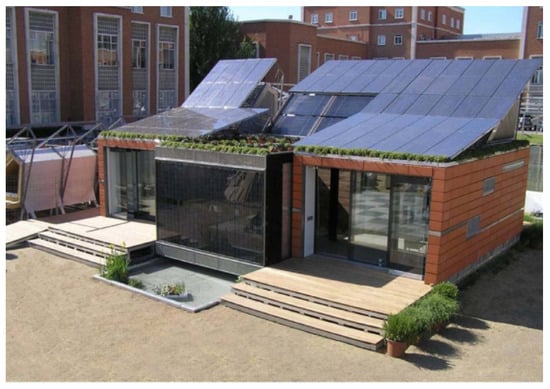
Figure 10.
Sendra et al. [83] use case: MagicBox, Technical University of Madrid, Spain.
In the same year, Correa et al. [84] employed deep learning techniques to predict the performance of a solar hot water (SHW) system under varying weather conditions in Chile. Using TRNSYS, a physical simulation model was created to generate a vast amount of simulated data. The different NN architectures received the ambient temperature, the solar field’s inlet temperature, the control signal of pumps (which is indicative of the operational status of the system’s pumps), the inlet temperature at the heat exchangers, as well as the previous values of the solar collector’s outlet temperature data. The primary aim was to predict the future values of the solar collector’s outlet temperature, and it portrayed a key performance indicator of the SHW system, thereby reflecting its efficiency and effectiveness in utilizing solar energy for heating water. Among the models tested, which included FNN, RNN, and LSTM architectures, the LSTM showcased superior prediction accuracy. When compared to traditional regression models, all three architectures, especially the LSTM models, delivered more reliable results, thus indicating their potential for predicting SHW system performance. More specifically, the LSTM model excelled in its predictions, achieving a low mean absolute error of 0.55 °C, the smallest root mean square error of 1.27 °C, as well as minimal variance and relative prediction errors.
In an interesting study in 2020, Heidari et al. [85] proposed advanced machine learning techniques for predicting the energy use in solar-assisted water heating systems by comparing multiple model architectures. The ANNs received input data as historical energy data; temporal variables like the hour and day; as well as environmental and operational Variables such as indoor and outdoor temperatures, solar radiation, relative humidity, and wind speed. The number of nodes in the input layer corresponded to the number of features used while the output layer of the models predicted the next time step of the energy use, thus making it a regression problem. To this end, multiple model architectures (LSTM, ALSTM, ALSTM-D, and FNN) were experimented on with different topologies, where the best performance was observed in a configuration with two LSTM layers containing 150 neurons in each hidden LSTM layer. The study compared the performance of the enhanced LSTM models—both with and without the attention mechanism and data decomposition—against a traditional FNN. The enhanced LSTM models demonstrated significantly lower mean absolute errors, and they outperformed the baseline FNN model by 25% to 41%, thus indicating a more accurate prediction of the energy use in solar heating systems.
In 2021, Tagliabue et al. [86] presented a technique that combined indoor air quality data, which were gathered from Internet of Things (IoT) sensors, to inform indoor environment changes based on how many people were present in a building at the University of Brescia’s Smart Campus (Figure 11). The method involved using a RNN that incorporates LSTM units trained on real-time data, which then guided the ventilation changes through an IoT communication system. The structure of the networks that utilized the CO2 in the air, the indoor temperature readings, and relative humidity (RH) data as inputs involved four hidden layers (recurrent LSTM, additional LSTM, sequence layer, and a fully connected layer). As its purpose was to predict the CO2 concentration as the output, the main goal of this research effort was to adjust the HVAC system and determine the optimal behavior for window operation in order to improve the indoor air quality. This, in turn, aimed to boost the cognitive performance of the building’s occupants, even as conditions changed. The research paper utilized Pearson’s correlation coefficient () with values of 0.93, 0.88, and 0.92 for the training, test, and whole datasets, respectively, as well as the mean square error (MSE) for the test period (which was approximately 10.6% of the average CO2 concentration).

Figure 11.
Tagliabue et al. [86] use case: eLUX lab, University of Brescia, Italy.
Also in 2021, Fang et al. [87] proposed a novel approach using a sequence-to-sequence model grounded in LSTM neural networks, which was employed for the advanced prediction of indoor temperatures and aimed to optimize the energy efficiency of HVAC systems. The model intricately processes a blend of historical indoor temperatures, as well as external factors such as forecasted outdoor temperatures and time-related data serving as the inputs. These inputs are skillfully encoded through LSTM layers for predicting the forecast horizon, which are adept at retaining important temporal information across sequences, thus ensuring a robust feature extraction. The model architecture consisted of a dynamic duo: an LSTM encoder that digests the input data, and an LSTM decoder that is fine tuned for generating accurate multi-step future temperature predictions. This architecture was fine tuned with hyperparameters such as the learning rate and number of hidden nodes, which were further reinforced with dropout techniques to curb overfitting. The models optimal prediction was determined for a single hidden layer with 128 nodes. Moreover, the efficiency of the approach prowess was benchmarked against established methods like Prophet and seasonal naive models, whereby it delivered superior performance in very short-term forecasting scenarios. What is noticeable is that their effort integrated a real-life application of this model, and it was tested in a real-world building environment (Figure 12) in order to showcase its potential in enhancing energy savings without compromising occupant comfort, thus marking a leap forward in intelligent building management systems.
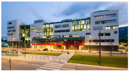
Figure 12.
Fang et al. [87] use case: GreEn-ER building, Université Grenoble Alpes, France.
4.3. Review of Hybrid Neural Networks Applications for BEMS Control
In an interesting hybrid study in 2015, Huang et al. [88] introduced a novel control approach for HVAC systems in commercial buildings, where the aim was to reduce energy use and costs. The approach combined a traditional MPC with an MLP and RNN (NARX) feedback method. The control model was based on a simplified representation, while the complexities in the HVAC process were addressed using an MLP structure that included three hidden layers and a single output node. More specifically, the MPL modeled the nonlinear input–output relationship of the building’s HVAC system, in which the system states (e.g., temperature) or control actions (e.g., valve positions) were predicted based on inputs like environmental conditions and desired output states. The MLPs received data that included the past and present values of various environmental and system parameters like the chilled water temperature, return air temperature, outdoor temperature, air mass flow rate, and the desired output while also predicting system states like temperature. The secondary employed RNN was a network able to capture the temporal dynamics of the building’s HVAC system, thus making it essential for accurately predicting system responses over time and aiding in the control process. The effectiveness of the methodology was evaluated at Adelaide Airport’s building using simulations and real-world settings, and this was achieved by incorporating such advanced air-conditioning strategies to optimize the energy efficiency. The results highlighted significant energy and cost savings of 13% without compromising comfort compared to the baseline control methods.
In a novel research effort in 2015, Papantoniou et al. [89] focused on enhancing energy efficiency in a hospital building in Chania, Greece by integrating a building optimization and control (BOC) algorithm into its existing BEMSs (Figure 13). The hybrid control approach integrates Elman RNN models for predictive modeling/temperature predictions, GAs for multi-step optimization, and fuzzy techniques for real-time control, all of which are aimed at enhancing energy efficiency in the building. With respect to the deployed RNN, it was aimed to predict indoor air temperatures, and it was trained with five real data inputs such as the indoor air temperature, time, convective transfer of windows, HVAC coil operation, and the HVAC fan consumption. The three hidden layers of the ANN consisted of 354 nodes each. Implemented within a web-based energy management and control system (Web-EMCS), the BOC algorithm effectively determines optimal temperature set points and monitors real-time data, such as energy savings. According to the real-life evaluation, the system demonstrated a potential energy saving of 36%.
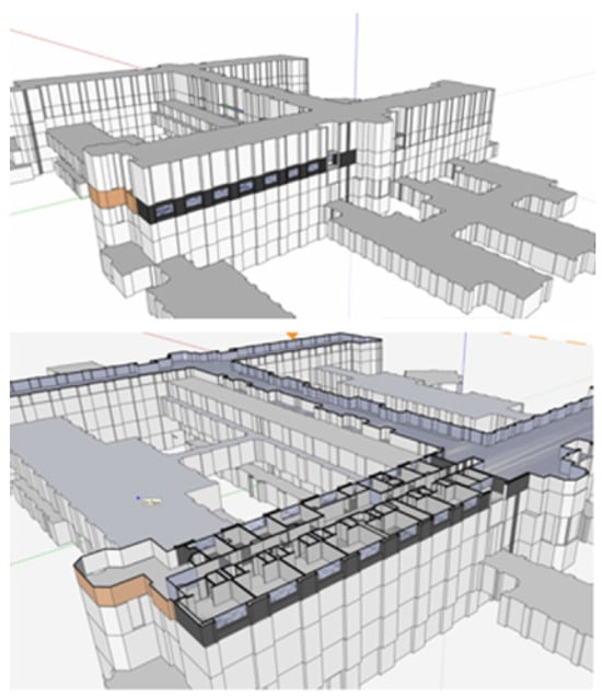
Figure 13.
Papantoniou et al. [89] use case: Saint George Hospital, Crete, Greece.
In the same year, Garnier et al. [90] proposed a novel predictive control approach targeting the enhancement of HVAC system operations in non-residential buildings. A building in Perpignan, France was modeled using EnergyPlus to gauge comfort using the predicted mean vote index. MLP served as the core of the predictive models that emulate HVAC system behaviors. The study used six self-growing ANNs, which were trained by the cascade-corellation algorithm to model variables like air and radiant temperatures, as well as the electrical power consumed by HVAC subsystems. As inputs, the models receive various parameters like the outdoor temperature, solar radiation, room occupancy, current air temperatures, radiant temperatures, and HVAC temperature set-points in adjacent rooms to predict the values of the air temperature, radiant temperature, and electrical power consumed by the building’s HVAC subsystems for each time step. The MLPs were developed for different operational modes (heating and cooling) and specific building areas. Such models were employed within an optimization framework powered by genetic algorithms (GAs), which efficiently dictate the optimal activation and deactivation times for HVAC components in both heating and cooling modes.
In 2015, Wei et al. [91] implemented an ensemble of multi-layer perceptron FNNs to develop an extensive energy model for a building. The model features a variable hidden layer, where the neuron nodes in the layer are randomly set between 10 to 40 during the training phase. It includes three indoor air quality models: the temperature model, the relative humidity model, and the CO2 concentration model. To balance the power consumption with the indoor air quality, a four-objective optimization problem was formulated. This challenge was tackled using an enhanced particle swarm optimization (PSO) algorithm, which determines control parameters for the supply air temperature and static pressure in the air management unit. By assigning different weights to the objectives within the model, the optimized control parameters effectively balanced the HVAC system’s power usage with the establishment’s thermal comfort. Simulation tests showed that the MLP ensemble method outperformed seven other techniques. It was thus selected for creating both the comprehensive energy model and the trio of indoor air quality (IAQ) models. The overall energy savings for the dataset in this study amounted to 17.4% without IAQ constraints and 12.4% under IAQ limitations for one of the eight user preference scenarios.
In 2016, Attaran et al. [92] proposed an innovative method for optimizing the energy efficiency of HVAC systems by combining a radial basis function neural network (RBFNN) with an epsilon constraint (EC) PID approach. This hybrid method employs RBFNN within the HVAC system to predict residual variances, which enhance the control signal and minimize errors. The primary objective was to design and evaluate the EC-RBFNN for a self-adjusting PID controller, and it is specifically tailored for a particular bilinear HVAC system with a focus on temperature and humidity control. Through comparative simulation case studies, the EC-RBFNN approach was found to be more accurate than both standard PID optimization and the combined PID-RBFNN method. The results showed that the hybrid EC-RBFNN methodology reduced the integral absolute error (IAE) by 18% for temperature and 20% for humidity measurements.
In the same year, Kim et al. [93] focused on improving the energy efficiency of integrated daylighting, heating, ventilating, and air conditioning (IDHVAC) systems in buildings. The researchers developed a meta-model to predict the building’s energy performance, which integrates artificial lighting regression and ANN models. This model was trained on a database generated by the EnergyPlus simulation tool, where the design of experiment (DOE) method is used to ensure robust training without overfitting in order to predict the room temperature, total energy consumption, and indoor daylight illuminance. The number of input variables for the ANN models varied depending on the specific model; meanwhile, the number of hidden layers was fixed at three for the ANN models and the number of neurons in each hidden layer was optimized using a genetic algorithm to minimize the total energy consumption while maintaining thermal and visual comfort for occupants. The GA optimization was applied to controllable variables within the IDHVAC system. According to the findings, which were based on three winter months of data, the GA-optimized IDHVAC system achieved an average energy savings of 13.7% compared to a conventional setup. When the optimization was applied separately to the HVAC system and Venetian blinds, the GA-optimized HVAC alone achieved 11.7% energy savings, while the combined IDHVAC optimization provided a higher savings rate.
In 2017, Yuce et al [94] proposed a novel framework for optimizing household energy management by scheduling appliances to operate at times that reduce peak energy demand while also maximizing the use of renewable energy. By integrating an ANN model—which was used to predict the energy demand and supply from RES along with a genetic algorithm (GA)—it was found to be adequate in receiving the predictions from the ANN, and it utilized them to create an optimized schedule for operating home appliances. With respect to the structure of the FNN, the inputs included environmental variables (outdoor temperature, wind speed, diffuse solar radiation, etc.), occupancy, appliance states, and time information. The remaining duration time for each appliance was an additional input. The outputs, on the other hand, included the total energy consumption, PV energy generation, and wind power generation—where the individual energy consumption for each appliance was also used as an output. The FNN used a single hidden layer, where the number of neurons in the hidden layer was determined experimentally. The best performance was found with 25 neurons. This smart scheduling led to a significant reduction in the grid energy consumption and shifted energy usage with respect to the periods with available RES energy, thus achieving more sustainable and cost-effective home energy use. The methodology was tested in a home environment, where it demonstrated reductions in grid energy dependence of 10%, 25%, and 40% on different occasions.
In 2019, Reynolds et al. [95] presented two different strategies for improving district energy management. The first focuses on enhancing the production of district heat from a multifaceted energy center, while the second combines this with direct control over building heating demand. The FNN models utilized the input data, such as the predicted outdoor temperature, solar irradiance, hour, day type, occupancy, the temperature set point, and the indoor temperature, of the previous hour. Each FNN integrated 2 hidden layers with 15 neurons per layer. One FNN predicted the hourly energy consumption, while the other predicted the hourly average indoor temperature. Such predictions were utilized with a genetic algorithm to determine the most efficient operation schedules for the heating equipment, thermal storage, and heating set points. The results showed a significant profit increase when optimizing heat production, as well as an even greater profit, as the system was adequate enough to adjust the building energy demand directly. According to the evaluation measurements, by focusing on optimizing the district heat production, there was a notable 44.88% profit boost compared to a standard rule-based strategy. When the system was also given the capability to directly influence the building energy demand, an extra 8.04% profit enhancement was observed.
Also in 2019, Satrio et al. [96] proposed a novel hybrid framework for enhancing the energy efficiency and thermal comfort of an educational building’s HVAC system (Figure 14). The researchers established a typical MLP to accurately predict the building’s energy consumption and the thermal comfort level of its occupants, as measured by the percentage of people dissatisfied (PPD) index. The structure of the FNN involved 10 input nodes—which received data such as the cooling set point, RH set point, starting delay, stopping delay, supply air flow rate (VAV system), window area, wall thickness, supply air temperature, supply radiant temperature, and supply radiant flow rate. The single hidden layer integrated three neurons, while the output layer included two output nodes for annual energy consumption and PPD predictions. By utilizing a multi-objective genetic algorithm (MOGA) framework, it was found to be adequate enough to generate the optimal operation settings for the building’s two-chiller HVAC system. The optimized system showed significant improvements in maintaining thermal comfort while also reducing annual energy consumption when compared to the baseline control operational settings.
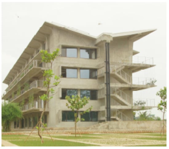
Figure 14.
Satrio et al. [96] use case: Educational Center, West Java, Indonesia.
In 2020, Bourhnane et al. [97] studied the prediction and management of energy consumption in smart buildings using machine learning techniques by employing FNNs in conjunction with GAs to model energy usage. The system was applied to a real-world setting, and it was used to process the data from a PV solar panel installation and various electrical appliances within the building. The networks were structured with 2 input neurons, a single hidden layer of 10 neurons, and a single output neuron. To this end, the model received two types of input: a timestamp of the energy consumption measurement and a unique identifier for each AC, fridge, furnace, and microwave appliance. The sole output of this model is the prediction of the energy consumption for each appliance. The evaluation illustrated that the hybrid FNN-GA approach showed the highest accuracy among all of the evaluated prediction methods that utilized the regression and the support vector machine models.
In a 2021 study, Elmaz et al. [98] introduced an advanced hybrid (CNN-LSTM) model. This model combines effective feature extraction with sequential learning to predict room temperature. The data from a room at Antwerp University was used to develop this control system. The hybrid CNN-LSTM network architecture comprised an input layer that received sensorial data from the motion detector (binary), as well as targeted set-point temperature, variable air volume (VAV) flow rate, window (binary), outside temperature, and room temperature data. The input layer is followed by two CNN layers for feature extraction. It then transitions to two LSTM layers to capture temporal dynamics, as well as uses a flatten layer to consolidate features. It then concludes with an output layer consisting of a single node dedicated to predicting temperature. The new approach was then benchmarked against the traditional MLP and a basic LSTM for short-term predictions spanning from 1 to 120 min. While all of the neural network models performed well for 1 min predictions, the CNN-LSTM model stood out in longer forecasts by consistently achieving an value greater than 0.9 for predictions up to 120 min.
In the same year, Somu et al. [99] proposed a novel transfer learning-based approach for the purpose of enhancing thermal comfort modeling in buildings, which is crucial for occupant well-being and productivity. To this end, a hybrid CNN-LSTM model was developed to capture the spatio-temporal relationships in thermal comfort data. The sophisticated model utilizes the data from thermal comfort parameters (TCPs) as the input, which includes the following: the indoor air temperature, indoor air temperature, indoor relative humidity, air velocity, mean radiant temperature, outdoor air temperature, as well as occupant age, gender, clothing insulation, and metabolic rate. The first hidden layer of the model is a 1D convolutional layer equipped with 128 filters and a kernel size of 5, which is followed by two LSTM layers, each with 256 nodes. Following the LSTM layers, the two fully connected dense layers respectively include 64 and 16 nodes. To this end, the five-node output layer provides model predictions of the different thermal comfort levels, which are categorized into a five-point thermal sensation scale (target classes: very cold/cold, slightly cool, neutral, slightly warm, and hot/very hot). The key modeling parameters for the TL CNN-LSTM model were determined using the Chi-squared test. At the same time, the issue of insufficient data samples across all of the thermal conditions was tackled using the synthetic minority oversampling technique (SMOTE). The model’s efficacy was tested on two source datasets (ASHRAE RP-884 and Scales Project) and a target dataset (Medium US office), and it demonstrated an accuracy of over 55% in the target buildings with limited data.
In their research work in 2021, Huang et al. [100] proposed an integrated ant colony optimization (ACO)-enhanced wavelet neural network (I-ACO-WNN) for the precise prediction of building heating and cooling loads. The model was assessed using key performance metrics, and it showcased its superior accuracy over traditional methods. Its WNN portrayed a special form of FNN using a wavelet basis function (WBF)—specifically the Mexican Hat wavelet—as its transfer function. The input layer received data that included eight building parameters: the relative compactness, surface area, wall area, roof area, overall height, orientation, glazing area, and glazing area distribution. The prediction of the network involved two output nodes, which represented the heating load (HL) and cooling load (CL) of the buildings. According to the evaluation, the regression coefficients for the heating load HL and CL predictions were 0.9714 and 0.9783, respectively. Compared to the standard wavelet neural network, the novel I-ACO-WNN model significantly reduced the prediction errors: the RMSE for HL and CL decreased by 66.01% and 73.28%, respectively; the MAE decreased by 82.44% and 84.82%, respectively; the MAPE decreased by 81.21% and 85.31%, respectively; and the MSE decreased by 88.44% and 92.86%, respectively.
In 2022, Afroz et al. [101] introduced a novel technique to curtail the energy use in HVAC systems, yet they also upheld the ambient internal standards as this necessitates extra power expenditure. The approach involved a complicated problem with several variables, which was resolved through a particle swarm optimization (PSO) algorithm. For regulating the internal indoor comfort and HVAC energy utilization, contemporary predictive formulations were established utilizing a nonlinear auto-regressive exogenous (NARX) neural network. The models utilized sophisticated information regarding multiple HVAC system and environmental parameters for the purpose of predicting the energy consumption, as well as indoor temperature, humidity, CO2, and VOC. NARX formulations underwent refinement to achieve the ideal forecast precision, and an ease of integration was conducted in the actual systems. To this end, the formulations were enhanced to determine the most efficient HVAC adjustments, which was achieved by considering seasonal alterations. The best performance was found with 12 hidden neurons and 2 time delays for the energy consumption prediction NARX, while the optimal NARX size for the indoor temperature, humidity, CO2, and VOC predictions were determined to be 10 hidden neurons and varying numbers of time delays (e.g., two or three). The outcomes revealed the feasibility of decreasing the overall power consumption by 7.8% without sacrificing internal conditions like the air warmth (19.60–28.20 °C) and moisture levels (30–65%).
4.4. Review of Other Neural Network Applications for BEMS Control
Javed et al., who also conducted a study in 2016 [102], proposed an intelligent HVAC controller that integrates IoT equipment, cloud computing, and web services. Using wireless sensors, the system is able to monitor the indoor conditions and control HVAC actuators. To this end, two random neural network (RandNN) models were employed to estimate the occupancy and set optimal HVAC operating points. The first model involved a five-node input layer that receives IoT sensorial data such as the room temperature, air inlet temperature, the CO2 environment, the CO2 inlet air, and the air inlet valve opening. Its single hidden layer consists of 10 nodes, while the output layer includes occupant predicting mean vote (PMV)-based setpoints for the purpose of HVAC control. With respect to the secondary RandNN, it similarly integrated five input nodes and received the data arising from IoT sensors such as the heating setpoint, cooling setpoint, heating error, cooling error, and CO2 level. The single hidden layer includes seven nodes, while the output layer integrates three nodes for the heating, cooling, and ventilation rates. It was noticeable that the training algorithm for both models involved a hybrid particle swarm optimization with a sequential quadratic programming (PSO-SQP) algorithm, and it showed a superior performance over the other methods. The results revealed that embedding the intelligence directly into the base station and sensor nodes reduced the power consumption by 4.4% compared to the storing data and running RandNN models on the cloud, as well as by 19.23% compared to the implemented RandNN models on the base station alone.
Also in 2017, Javed et al. [103] introduced a novel concept involving the integration of decentralized smart controllers within an Internet of Things (IoT) framework, one that is enhanced by cloud computing for training random neural networks (RandNNs). This setup was designed to monitor variables such as temperature, humidity, HVAC airflow, and passive infrared sensor (PIR) data. The advanced controller system consists of three key components (each endowed with specific functions): a base station, sensor nodes, and cloud-based intelligence. One of the notable features was a sensor node equipped with a RandNN-based occupancy estimator (a PMV-based setpoint estimator) that can estimate the number of occupants in a room and relay this information to the base station. The base station, in turn, utilizes RandNN models to control the HVAC system, where it adjusts it based on the established setpoints for heating and cooling. The structure of the first RandNN (a PMV-based setpoint estimator) utilized PMV and humidity as the inputs while the single hidden layer consisted of four neurons directing information to the single output node in order to predict the relative temperature setpoint. The secondary RandNN exploited information regarding the heating setpoint, cooling setpoint, and heating error (i.e., the difference between the heating setpoint and the current temperature) in order to align the HVAC operations with the desired temperature setpoints, which were either estimated by the RNN PMV model or set by the user. Such real-life implementation was compared to basic RBC controllers, and the study illustrated the adequacy of the RandNN controller in reducing HVAC energy consumption by 27.12%.
5. Evaluation
5.1. Evaluation per Utilized Data
Building energy management systems (BEMSs) integrate a variety of input data for ANN applications, where each component plays a critical role in enhancing the accuracy and reliability of predictions. To this end, HVAC applications commonly utilize indoor and outdoor temperature and humidity levels; air quality; occupancy levels and patterns; time of day; and seasonal information, as well as historical data on energy consumption and temperature settings to generate decisions for optimizing HVAC settings or energy consumption forecasts [61,65,66,72,88,89,90,91,92]. Similarly, DHW system operations also depend on similar aspects such as the incoming water temperature, historical energy consumption for water heating, water usage patterns (e.g., peak usage times), or ambient temperature and weather conditions. Such elements are commonly utilized to generate predictions such as the energy requirements for water heating and predicted hot water demand, or to provide optimized decisions for water heating schedules [62,79]. ANN models that include LSs on the other hand, most commonly utilize data that consider occupancy patterns and illuminance levels to predict lighting power settings [66]. Last but not least, RES is most commonly utilized with climatic and radiometric data, as well as solar irradiation, wind speed, and ambient temperature parameters to forecast renewable energy production, availability, and variability at the building level [63,71,75,82,84,94,97].
Figure 15 illustrates the potential occurrence of the different data founded in the majority of the integrated works (left) while also illustrating the occurrence (%) per different data types that integrate the following different types of data: environmental (e.g., temperature, humidity, wind speed, solar radiation, CO2 levels, air Quality Data, etc.); operational (energy usage and operational status); behavioral (behavioral patterns, presence and count of occupants, historical timestamps, etc.); and other data (right).

Figure 15.
Occurrence per different types of data (left) and the data type occurrence (%) in highly cited BEMS applications (right).
It should also be noted that the nature and characteristics of the available data for processing strongly affect the selection of the suitable ANN type. For instance, it is evident that FNN structures are typically employed in scenarios where the relationship between the input and output of the model is static, thus making them ideal for pattern recognition tasks where the sequence of data points is not crucial. They are adept at handling various data types, including static, numerical, categorical, and non-sequential data. This makes FNNs suitable for applications in BEMSs, such as predicting the energy consumption of HVAC systems and LSs based on current conditions, occupancy, and building characteristics. On the other hand, RNNs excel in scenarios where the sequence and context of data are vital. They are designed to process sequential and time series data, which is essential in applications like predictive maintenance or energy load forecasting in BEMSs. RNNs are more than adequate for analyzing the historical data patterns, including energy usage over time and weather conditions, required to make informed predictions about future loads or maintenance needs [86,87]. Moreover, the complexity and structure of the data also play a crucial role. More complicated data with higher dimensionality might require advanced architectures like DNNs for more effective feature extraction and learning. Such networks integrate multiple hidden layers, and they are able to unravel complex patterns and relationships within large and multifaceted datasets; thus, they enable more effective and accurate predictions [70,74]. In contrast, simpler data structures may be efficiently handled by less complex models [59,61,63,64,68,71,75]. Such fundamental differences in data handling between the different types of networks underline their distinct roles in various applications within the domain of building energy management. The following subsection thoroughly analyzes the distinct role of the different types of ANNs that are found in the literature related to BEMS applications.
5.2. Evaluation per ANN Type
The selection of ANN types for different BEMS applications is largely influenced by the specific characteristics and requirements of the systems being controlled, like HVAC systems, DHW systems, LSs, and RESs.
MLPs, a type of FNN, are commonly chosen for BEMS applications due to their straightforward architecture and efficacy in handling a range of prediction and classification tasks. Such an ANN type is largely favored in BEMS applications, especially in cases where the relationship between input and output is more direct and less influenced by temporal factors—i.e., where the operational patterns are relatively predictable and do not involve complex temporal dynamics. For instance, in managing DHW systems and certain aspects of LSs, where the demand patterns are more consistent and predictable, MLPs are adequate due to their ability to model these relationships without the need for understanding sequential data. The advantage of MLPs lies in their simplicity and efficiency, i.e., in offering a straightforward approach to modeling. However, this simplicity also translates to a limitation, as MLPs lack the capability to process time series data effectively, thus making them unsuitable for applications that require understanding historical patterns and predicting future trends. In order to overcome such limitations, RNNs—particularly LSTMs—have been extensively utilized in the literature toward complex BEMS tasks like HVAC control and RES management. HVAC systems, with their variable and dynamic operation, require an approach that considers historical data to predict future needs. LSTMs are well equipped for this given their ability to remember and leverage long-term dependencies in data, a crucial feature for accurately predicting energy needs based on past trends. This capability is equally important in managing RESs, where factors like weather conditions and energy generation from sources like solar panels are highly variable and dependent on historical patterns. It should be mentioned that LSTMs are generally considered superior to traditional RNNs because they effectively overcome the vanishing gradient problem, which enables them to learn from long-term dependencies in data. This feature makes LSTMs adept at handling complex sequences where understanding past context is crucial. Additionally, LSTMs maintain a more stable and consistent training process, thus leading to better performances in tasks involving sequential data. However, the depth of LSTMs comes at the cost of increased computational complexity and data requirements. They need extensive and diverse datasets for training to capture the nuances of these complex systems. This might not be a significant issue for commercial buildings, where such data are more readily available, but they can be a challenge in smaller-scale applications.
Figure 16 illustrates the occurrence per ANN type (left), as well as the citation share (%) per ANN type (right), in highly cited BEMS applications.
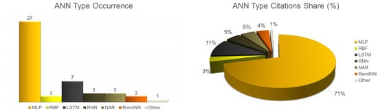
Figure 16.
Occurrence per ANN type (left) and citation share (%) per ANN type (right) in highly cited BEMS applications.
Another fruitful approach is in deploying BEMS control concerns to hybrid schemes, where ANNs are integrated with other algorithms or approaches to harness the combined advantages of the methodologies. According to the literature, the most prominent combination, considering the research interest, concerns the integration of ANNs with genetic algorithms [89,90,93,94,95,96,97]. This type of integrated scheme is common due to the complementary strengths of these two methods. GAs, inspired by the process of natural selection, excel at exploring a vast solution space and finding global optima, thus making them ideal for optimizing the structure and parameters of ANNs, which can be a complex, multi-dimensional problem [90,93,94]. This combination enhances the ANN’s ability to learn and adapt, especially in complex, non-linear environments where traditional gradient-based methods might struggle. Moreover, GAs have been thoroughly utilized for the scheduling and operational optimization of BEMSs [95,96], as well as in handling multi-objective problems such as balancing energy usage with comfort and exploring complex solution spaces [89,97]. Similar to GAs, PSOs that are integrated with ANNs leverage swarm intelligence for efficient parameter optimization, thereby enhancing a network’s performance in discovering optimal or near-optimal solutions. In [91], the role of PSOs was to find a balance between power usage and indoor air quality, in which the trade-offs were effectively managed between these competing objectives.
In the literature, there is also the neuro-fuzzy approach, which combines fuzzy logic controllers (FLCs) with ANNs. It capitalizes on the ANN’s learning capabilities and the intuitive, human-like reasoning of fuzzy logic, thus making it particularly effective for handling uncertainty and imprecision in data [98]. Other notable combinations found in the recent literature include ANNs with simulated annealing for robust optimization in complex landscapes, as well as ANNs with RL, which is pivotal in decision-making scenarios and adaptive systems that learn from interactions with their environment. These hybrid models underscore the trend of leveraging the strengths of various algorithms to offset the limitations of standalone methods, thus leading to more powerful, adaptable, and efficient problem-solving tools.
5.3. Evaluation per Training Scheme: Optimization Algorithms and Training Methodologies
The prevalence of the gradient descent approach using the backpropagation (GD/BP) method in training neural networks for BEMSs is largely due to its proven effectiveness, simplicity, and adaptability to a wide range of problems [62,64,69,74,80,82,83,84,86,98]. GD/BP is straightforward to implement and flexible enough to handle the diverse nature of BEMS applications, which often involve complex datasets. Such a scheme is potentially favored due to its computational efficiency, a crucial factor when handling large-scale data, thus making it a widely chosen option. On the other hand, the Levenberg–Marquardt (LM) method combined with backpropagation (LM/BP) has also emerged as a prevalent methodology as it is favored for its faster convergence in smaller networks or its well-behaved loss functions [63,73,75,79,81,93,95]. However, LM’s higher computational demands in large-scale applications has limited its wider adoption compared to GD/BP training and optimization methodologies with respect to training ANNs in BEMS applications.
Furthermore, variations like /BP, GD/BP with momentum (GD/), or Bayesian Regularization have been employed to address specific challenges in neural network training within BEMSs. For instance, the Adam optimizer in the gradient descent approach adapts learning rates for each parameter and offers improvements in complex scenarios [74,98]. Momentum in backpropagation helps accelerate convergence and navigate the optimization landscape more effectively [71,80,82], while Bayesian regularization in backpropagation enhances the model’s generalization capability, an essential trait for reliable performance in diverse BEMS scenarios [66,70,80].
What is noticeable for training RNNs is the common use of the gradient descent approach through time combined with backpropagation (/BP). Such a tendency is deeply rooted in the temporal characteristics of these systems. BEMS applications often involve time series data, such as energy consumption patterns, environmental conditions, and user behaviors, which exhibit significant temporal dependencies. RNNs are uniquely suited for this type of data due to their ability to maintain and learn from historical information over time. The (/BP) approach is particularly effective here, as it adapts the gradient descent optimization to work across time sequences, thus ensuring that the network’s learning process takes into account the entire temporal context of the data [82,83,84,86]. This ability to capture and utilize temporal dynamics is crucial for accurate modeling, forecasting, and decision making in BEMSs, thereby making (/BP) a preferred choice for training RNNs in these applications. Such an integrated approach allows RNNs to learn from dependencies and patterns that span across time steps, which is essential for accurately modeling and predicting temporal dynamics.
With respect to random neural networks, it should be noted that the use of particle swarm optimization (PSO) combined with sequential quadratic programming (SQP) (RandNNs) harnesses the global search capability of PSO and the precise local optimization of SQP. This method is particularly effective for RandNNs due to their stochastic nature and complex optimization landscapes. PSO efficiently explores the broad solution space to identify promising regions, while SQP fine tunes the solutions, thus ensuring optimal network weights are achieved. This combination is ideal for addressing the unique challenges posed by RandNNs, especially in scenarios where traditional gradient-based methods may fall short [102,103].
Figure 17 portrays the occurrence per optimization algorithm (left) and the occurrence per training methodology (right) in highly cited BEMS applications.

Figure 17.
Occurrence per optimization algorithm (left) and occurrence per training methodology (right) in highly cited BEMS applications.
5.4. Evaluation per Transfer Function
In FNNs, the preference for specific activation functions is influenced by their distinct characteristics and the network’s architectural requirements. The sigmoid (sig) function is the most common in hidden layers due to its smooth, nonlinear nature, which allows for gradient-based optimization and helps the network capture complex patterns in the data (as shown in Figure 18, where its output range (0 to 1) is particularly useful in binary classification tasks).
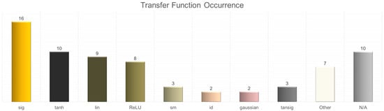
Figure 18.
Occurrence per transfer function in highly cited BEMS applications.
Tanh (hyperbolic tangent function) is the second most common function in FNN structures. It is also preferred for its output range (−1 to 1) as it offers a centered zero mean, which can lead to faster convergence during training. Tanh is commonly used in output layers when the task requires mapping to a bipolar output [69,91]. This is also the case for the linear (lin) function, which is predominantly used in the output layer and portrays a crucial factor for tasks where the goal is to predict continuous and unbounded values, such as in regression problems [60,63,66,83,88,90,93]. The linear function operates in a linear nature, and it allows the network to output a range of values without applying a nonlinear transformation, thus making it suitable for such tasks. The choice of activation functions in FNNs is strategic and aimed at optimizing the network’s learning and predictive abilities. The sigmoid function’s role in hidden layers is to introduce nonlinearity, which is essential for learning complex functions [66,69,70,77]. Meanwhile, the linear or tanh functions in the output layer cater to the specific nature of the network’s output, whether it is classification, bipolar mapping, or regression. This strategic selection ensures that the network’s architecture is aligned with its intended function and the nature of the data it processes.
In RNNs, activation function preferences differ from FNNs due to RNNs’ unique structure and sequential data processing. Tanh is often used in RNN hidden layers for its range (−1 to 1) and effectiveness in mitigating the vanishing gradient problem, which is crucial in RNN training [83,84]. ReLU and its variants are also employed for their fast training capabilities and non-linear representation [80], which help to address gradient issues. Sigmoid functions are less common in RNN hidden layers, but they are utilized in specific parts of LSTM networks for their gating mechanisms. For output layers, linear activation functions are used in RNNs for tasks requiring continuous value predictions, similar to FNNs [79,83]. The selection of activation/transfer functions in RNNs are thus heavily influenced by their architecture and the sequential nature of their tasks.
5.5. Evaluation per ANN Depth
The use of ANNs in BEMSs is especially influenced by the complexity and specific requirements of the systems they are designed to control. To this end, the depth of the ANN (denoted as the number of hidden layers) portrays a crucial consideration for each research work. Shallow ANNs, i.e., those holding a single hidden layer, are generally sufficient for less complicated BEMS frameworks or where data are limited. Such ANNs are quicker to train and require less computational power. In contrast, deep ANNs, which have multiple hidden layers—typically 2–4 layers—in BEMS applications, are capable of capturing more complex patterns and interactions in data. This renders them more suitable for intricate systems like advanced HVAC controls or integrated RESs, where multiple variables and non-linear relationships must be considered.
The specific BEMS component being controlled may also dictate the ANN design. For example, controlling a lighting system [66] might not require the depth and complexity needed for an HVAC system, where factors like occupancy variability and energy storage play a significant role [62,65,70,74,86,88,89,98]. Similarly, DHW systems might need a different approach compared to HVAC systems, as the latter often involves more dynamic and complex control strategies [79].
According to the evaluation denoted in Figure 19, shallow ANNs more commonly appear as FNNs [59,61,63,64,66,68,69,71,75]. Such a tendency may be interpreted as being present due to the fact that many BEMS tasks do not require the sophisticated temporal data processing that deep RNNs offer [81,83,85,86]. Single-layer FNNs are computationally less intensive and easier to train, thus making them suitable for applications with simpler, more direct data relationships. Thus, they are preferred in scenarios where the focus is on achieving quick, efficient processing with less emphasis on capturing complex, long-term data dependencies.
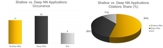
Figure 19.
Occurrence of shallow and deep ANN applications (left), as well as the citation share (%) of shallow and deep ANN applications (right), in highly cited BEMS applications.
In summary, the choice between shallow and deep ANNs, as well as the selection of a particular architecture in BEMSs, are dictated by the specific characteristics and requirements of the system being managed. This includes the complexity of the system, the nature of the data involved, and the precision required in control and prediction.
5.6. Evaluation per Computational Complexity
Evaluating the computational demand of ANN architectures, especially in the context of BEMSs, involves a comprehensive approach that considers several intrinsic factors related to neural network design and functioning. The complexity of a neural network is determined not only by its size, but also by the architecture and the characteristics of its components. For instance, the number of hidden layers in a network plays a critical role in determining the computational complexity of the ANN model. Networks with more layers represent more complex functions, but this comes at the cost of increased computational requirements for both training and inference phases [74,87,101]. To this end, the depth of the network directly correlates to the volume of computations needed. Another crucial aspect considers the number of neurons per layer. An increased count of neurons leads to a greater number of weights and biases within the network, and this consequently escalates the computational load. While more neurons enable the network to capture complex patterns, it also requires additional computational resources [78].
The type of neural network portrays another significant factor. Different architectures have varying computational demands. For instance, RNNs, particularly LSTM networks [86,87], require advanced complexity compared to standard FNNs [59,63,64]. Such complexity arises from their ability to handle sequential data, and this is attributed to their recurrent connections. Additionally, the complexity of the activation functions used within the network also affects the computational load. Some activation functions, like, e.g., sigmoid and tanh [70], involve more complex mathematical operations than simpler functions like ReLU [67]. The choice of activation function can, therefore, have a non-trivial impact on the amount of computation required.
It should be also noted that hybrid models, which combine different neural network types, exhibit higher complexity [98,99]. This increased complexity is due to the integration of computational demands from each of the component models. Furthermore, the methods used for training the networks and the optimization algorithms employed add layers of complexity. Last but not least, training methods like backpropagation with a gradient descent approach—or with variations such as stochastic gradient descent, momentum, or adaptive learning rate methods—hold different computational demands.
Grounded in the aforementioned attributes, this paper justifies the computational complexity of each case scenario. Figure 20 and Figure 21 illustrate an estimation of the integrated computational demand of each FNN, RNN, and hybrid approach. (Cases where the computational estimation was not feasible to determine have been excluded from the justification, such as, e.g., cases with varying number of layers or nodes.) These estimations were conducted according to the number of hidden layers; number of neurons per layer; type of neural network; complexity of activation functions; hybrid models; training methods; and optimization algorithms.

Figure 20.
Computational complexity estimation for Feedforward neural network cases [59,60,61,63,64,65,66,67,69,70,71,72,73,74,76,77,78].

Figure 21.
Computational complexity estimation for recurrent neural networks (right) [79,80,81,82,83,84,85,86] and hybrid cases (left) [87,88,89,90,91,92,93,94,95,96,97,98,99,100,101].
5.7. Evaluation per Statistical Index Utilization
In order to evaluate the most prevalent statistical indexes for illustrating the performance of a potential ANN model, the current work thoroughly examined instances of highly cited research works. According to the evaluation depicted in Figure 22—right, the most prevalent statistical index types include the following error metrics that provide accuracy in predictions: the RMSE (root mean square error), the MSE (mean squared error), the MAPE (mean absolute percentage error), and the MAE (mean absolute error). Figure 22—left includes the most prominent indexes that are commonly utilized in the literature. The RMSE and MSE are widely used since they emphasize larger errors by squaring the residuals, thus making them particularly sensitive to outliers, which is crucial in energy management where extreme values can have significant implications. The MAPE is also popular due to its ability to express errors as a percentage, and it offers a clear and relatable perspective on model accuracy, which is especially useful in communicating results to non-technical stakeholders [59,61,64,69,71,75,76,82,91]. Also, the MAE provides a direct average measurement of error magnitudes, thus making it intuitively easy to understand and interpret [59,61,84,85,98].

Figure 22.
Occurrence per statistical index (left) and citation share (%) of the statistical index types (right), in highly cited BEMS applications.
Moreover, the utilization of correlation metrics such as (i.e., the coefficient of determination) is also significant, as shown in Figure 22—right, due to their efficiency in capturing different aspects of model performance [60,63,69,71,76,82,84,86,89,96,98]. The metric indicates the proportion of variance in a dependent variable that is predictable from independent variables, and it provides a measure of how well unseen samples are likely to be predicted by the model. Standardization and normalization metrics such as the standard deviation (std) [59,91] and the coefficient of variation (CV) [59,60,64,72,93] are less common in ANN-BEMS research as they primarily measure data variability rather than model prediction accuracy. This means they are not complementary to the main focus of evaluating ANN performance in energy management tasks.
Such indices collectively offer a comprehensive view of an ANN’s performance, where accuracy, error magnitude, and the model’s ability to explain variability in the data are covered. Their widespread adoption in BEMS applications reflects a standardized approach to model evaluation and facilitates comparisons between different studies and models; in addition, their utilization ensures a thorough and nuanced understanding of the model’s predictive capabilities, which is essential for effective energy management and decision making in BEMSs.
5.8. Evaluation per BEMS Type
According to the evaluation shown in Figure 23, HVAC systems are predominantly featured in the ANN applications for BEMSs. Such a tendency is explained by the fact that HVAC systems most commonly involve the largest consumers of energy in buildings in comparison to other BEMSs. Moreover, HVAC systems are thus predominantly featured in ANN applications for BEMSs due to their complex operational dynamics and high energy demand. Such BEMS types present a multifaceted control challenge in being integrated with other building systems and the external environment—a task ANNs are sufficient enough to address by processing large data amounts from diverse sources. Additionally, the trend toward smart buildings and IoT integration has increased data availability on HVAC performance, thus boosting ANN learning and adaptation potential for HVAC control. This aligns with the regulatory and sustainability goals driving advanced technologies like ANNs for energy conservation.
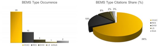
Figure 23.
Occurrence per BEMS type (left) and citation share (%) per BEMS type (right) in highly cited BEMS applications.
RESs are also increasingly being utilized in ANNs for BEMSs due to their role in sustainable energy management [63,71,75,76,81,84,94,97]. ANNs manage the unpredictability of RESs for parameters like solar and wind power, and they aid in enhancing energy generation and usage. They are crucial for balancing intermittent RESs, optimizing energy storage, and integrating RESs with conventional systems, thus supporting net-zero buildings and carbon neutrality goals.
In contrast, DHWs [60,62,79] and LSs [66] are less featured in ANN applications due to their simpler operational dynamics and more predictable patterns, which thus require less complex data processing. Their lower energy consumption and limited data availability make simpler control methods more cost effective, thereby leading to their infrequent use in advanced BEMSs. BEMSs often prioritize more complex systems like HVAC systems and RESs for greater energy saving and efficiency.
Last but not least, it should be mentioned that IBEMS applications are also limited [80,93] probably due to the intricate coordination required, whereas approaches such as DRL are preferred in such sophisticated systems.
5.9. Evaluation per Building Testbed Type
Commercial buildings are more commonly the focus of ANN applications in BEMSs compared to residential buildings primarily due to their larger scale and complexity. Commercial buildings, such as office complexes, shopping centers, and hotels, often have more varied and intensive energy needs, thereby providing a broader scope for optimization and efficiency improvements when using ANNs. The diversity in usage patterns, occupancy rates, and energy systems in commercial buildings presents a rich dataset for ANNs to analyze and learn from, thus making them ideal candidates for advanced energy management research.
Additionally, the potential for energy savings and cost reductions is generally higher in commercial settings due to their larger energy consumption. This makes the investment in sophisticated ANN-based BEMSs more financially justifiable for commercial properties. Moreover, commercial buildings often have more resources and infrastructure to implement and benefit from advanced technologies like ANNs. Lastly, commercial buildings are subject to stricter regulatory and sustainability mandates; therefore, they drive the adoption of innovative energy management solutions like ANNs to meet these requirements. This combination of factors contributes to the higher research interest and prevalence of ANNs in commercial BEMS applications. The predominance of ANN applications in commercial buildings, as opposed to residential ones [59,68,81,94,97], is clearly illustrated in Figure 24. Both graphs effectively showcase the trends in occurrence and research interest, and they also highlight the significant focus on commercial settings for ANN implementations in BEMSs.
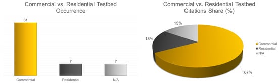
Figure 24.
Occurrence per building testbed type (left) and citation share (%) per building testbed Type (right) in highly cited BEMS applications.
6. Current Trends and Future Directions
6.1. Trend Identification
According to the evaluation, the selection of the ANN type for such optimization tasks is strongly influenced by the characteristics and requirements of the targeted energy management system. To this end, MLPs, which are empowered by a straightforward implementation, illustrate the dominant ANN architecture applied in both simple, as well as in more elaborate, BEMS frameworks. However, for elaborate tasks requiring training toward large-scale time series historical data, ANN types such as RNNs—especially LSTMs—present an advantageous alternative. MLPs are also dominant in hybrid applications, where their integration with evolutionary algorithms—such as GAs and PSOs—are increasingly used to enhance learning and adaptability in complex environments. Neuro-fuzzy approaches are also present in the literature for the purpose of integrating fuzzy logic with ANNs, specifically for handling uncertainty and imprecision in data. With respect to the depth of the deployed ANN per applications, it should be mentioned that such attributes are elected—or experimentally determined—based on the system’s complexity. Shallow ANNs are sufficient for simpler frameworks, whereas deep ANNs, which feature multiple hidden layers, are suitable for complex systems like advanced multi-BEMS controls or integrated RESs. In general, hyperparameter optimization is considered another meaningful research objective for multiple research applications that concern ANNs in BEMSs.
In terms of optimization algorithms and training methodologies, the popular gradient descent algorithm deployed in the backpropagation (GD/BP) methodology is prevalent in BEMS applications due to its effectiveness and computational efficiency. Variations such as the optimizer, (BP with momentum), or (BP with Bayesian regulation) cater to specific challenges in neural network training. Particularly for training RNNs, it is noticeable that the (gradient descent through time) algorithm is widely used, especially for handling temporal data characteristics in BEMSs. The activation or transfer functions that are utilized in FNNs and RNNs are strategically chosen based on their distinct characteristics and the network’s architectural requirements. Sigmoid functions are common in the hidden layers of FNNs, while tanh and linear functions are deployed to specific tasks in output layers. In RNNs, the tanh function is often used in hidden layers to mitigate the vanishing gradient problem, while ReLU variants are employed for faster training.
With respect to the typical cost functions for evaluating ANN model performance, statistical indices are commonly used, including certain error metrics like the RMSE, MSE, MAPE, and MAE, which focus on the accuracy of predictions and error magnitude. The use of correlation metrics such as is another widely utilized approach as they are specialized for capturing different aspects of an ANN model’s performance. Regarding the types of BEMSs, HVAC systems are predominantly featured, followed by RESs due to their complex operational dynamics challenges and significant energy demand requirements in buildings. Conversely, systems like DHW and LS are less emphasized due to their simpler operational dynamics and more predictable patterns. Finally, commercial buildings are more commonly the focus in ANN applications compared to residential buildings due to their larger scale, complexity, and higher potential for energy savings. The diverse usage patterns, occupancy rates, and energy systems in commercial buildings provide a broad scope for optimization and efficiency improvements when using ANNs, and this is further driven by stricter regulatory and sustainability mandates.
6.2. Future Directions
As we look toward the future of ANNs in BEMSs, several key directions emerge that researchers are likely to pursue in order to optimize their efficiency and effectiveness. One of the foremost areas concerns the enhancement of data preprocessing techniques. This involves developing more sophisticated methods for cleaning, normalizing, and segmenting time series data, thereby ensuring that the data fed into ANNs are highly relevant. This step is crucial because the accuracy of ANNs largely depends on the quality of input data. For instance, employing innovative strategies like outlier detection and missing data imputation to identify and correct data errors or min-max normalization may prove quite beneficial. Moreover, partitioning time series data is also a key aspect in preprocessing, which can be performed based on time intervals or specific events via utilizing approaches like the sliding window technique. Additionally, feature engineering, including time series decomposition and the creation of derived features, may potentially expose relevant patterns and trends in the data.
Regarding this same aspect, the efficient integration of multi-source data into ANNs also represents a significant future direction. By combining the information from various sources like weather forecasts, occupancy sensors, and historical energy usage data, ANNs can help with gaining a more holistic understanding of building energy dynamics. To this end, future research needs to focus on aligning diverse datasets like weather forecasts, occupancy sensors, and energy usage history, thus ensuring compatibility through preprocessing methods, such as normalization. Ensemble learning, i.e., combining multiple models that are trained on different datasets, will also be explored to enhance prediction accuracy.
Ensuring the scalability of ANNs is another critical area. As buildings become more complex and interconnected, the ANNs used in BEMSs must be capable of scaling accordingly. This means they should handle larger and more diverse datasets without a loss in performance or efficiency. The trend of using deep ANNs for more complex BEMSs is aligned to future directions when emphasizing the scalability of ANNs. Deep ANNs have the advantage of being able to model complex, non-linear relationships, thus making them well suited for the multifaceted challenges of modern and future BEMSs, which includes integrating RESs, dynamic occupancy patterns, and varying environmental conditions. To this end, deep architectures, which are characterized by multiple hidden layers, will be more effective in capturing the intricate patterns and dependencies in the data; thus, they will become more prevalent in research.
To this end, the improvement of training algorithms will also be essential in order to efficiently train deep architectures. Researchers need to intensively focus on developing algorithms that are adequate for training DNNs more efficiently, i.e., where the aim is to reduce the time and computational resources required while also minimizing the risk of overfitting. The prevalent use of the gradient descent method and its variations, like GD through time () for RNNs, aligns with the future emphasis on improving training algorithms. Optimizing these algorithms is key to efficiently training DNNs, especially as they grow in complexity and scale. Such enhanced algorithms would enable ANNs to learn from BEMS data more effectively, thus making them more accurate and reliable in their predictions and decisions. Moreover, addressing computational efficiency is vital for the practical deployment of ANNs in BEMSs. This involves optimizing the algorithms and computational processes used by ANNs so that they can operate effectively (even in resource-constrained environments).
In parallel, tailoring the architecture of ANNs to suit the specific needs of BEMS data will be a focus area. This might involve the selection of the appropriate ANN Type, the architecture design of the network, the utilization of advanced techniques, hyperparameter optimization, as well as the continuous testing and validation of the models toward real-world data. In the future, ANN research for BEMSs will likely need to focus on more innovative ANN types and architectures to handle the increasing volume and complexity of time series data. This will potentially include a greater emphasis on RNNs, particularly LSTMs, for their superior ability to process sequential data. Additionally, attention mechanisms and transformer models, known for their effectiveness in handling long-range dependencies in time series, may play a significant role. The expansion and complexity of data will further necessitate exploring more innovative hybrid models that combine the strengths of different architectures—e.g., neuro-fuzzy approaches—which will have to be achieved by ensuring both efficiency and accuracy in handling diverse building energy management scenarios. Beyond the selection of more suitable ANN architecture, the customization of ANN structure so as to better suit the specific characteristics of energy and environmental data may foster the development of ANN architectures that are specifically tuned to the complex demands of BEMSs, thereby resulting in more accurate and efficient energy management systems.
Moreover, a promising direction for future research would be to explore the interplay between ANN prediction uncertainties and the efficiency of control strategies in BEMSs. Specifically, an investigation on the integration of ANN models within MPC systems, in conjunction with feedback controllers, would impact the overall energy optimization. There is a delicate balance to be struck here: while feedback mechanisms can compensate for prediction inaccuracies, they might also reduce the energy savings achieved through optimization. Hence, future studies should also focus on a comprehensive evaluation that encompasses the total energy savings by considering both the predictive accuracy of ANN models and the effectiveness of feedback adjustments in maintaining operational conditions like temperature. Such a holistic approach could yield insights into optimizing ANN-based BEMSs for enhanced energy efficiency while accounting for uncertainties.
Another important direction is related to the incorporation of real-time learning capabilities into ANNs. To incorporate real-time learning into ANNs for BEMSs, the focus will be on implementing online learning, where the model continuously updates with new data. This involves setting up systems to process data streams efficiently by employing incremental learning to prevent loss of prior knowledge, as well as for establishing feedback loops for adaptive responses. Real-time data augmentation and utilizing edge computing are crucial for handling live data variations and reducing latency. Additionally, developing strategic model update protocols and ensuring a robust infrastructure are essential. These steps will enable ANNs to dynamically adapt to immediate changes in energy usage, occupancy, and environmental conditions in real time.
Lastly, ensuring data security and privacy in the use of ANNs will be paramount. As ANNs handle sensitive information about building operations and occupant behavior, safeguarding this data against breaches is crucial. This includes encrypting data both in transit and at rest, using secure protocols for data transmission, and applying rigorous access controls. Regular security audits and updates to address emerging threats will be essential. Additionally, incorporating privacy-preserving techniques like differential privacy, where individual data points are obscured to protect user identity, will be key. Researchers will also focus on compliance with data protection regulations to ensure that the handling of sensitive information about building operations and occupant behavior is both secure and legally sound.
7. Conclusions
The current review was focused on the examination and analysis of the most impactful research of recent years (2015–2023) with respect to the applications of ANNs toward BEMSs. By thoroughly investigating numerous research applications, the primary aim of this work was to deliver a summarized overview of such a framework and to deliver to the interested reader the trends, potential, and future directions in the current field.
According to the evaluation, the current trends in ANN applications for BEMSs reveal a nuanced approach to selecting appropriate ANN types and architectures. The use of shallow ANNs in simpler BEMS tasks, and the shift toward more complex structures like deep MLPs and RNNs, particularly LSTMs, for handling dynamic and time-sensitive BEMS tasks, underscore the need to match ANN architecture with a system’s specific requirements. This trend is anticipated to continue with an increasing emphasis on tailoring ANN architectures to suit the unique demands of BEMS data. In terms of optimization algorithms and training methodologies, the prevalent use of the gradient descent approach and its variations for training ANNs in BEMSs is likely to evolve. Future advancements are expected to focus on developing more efficient training algorithms and enhancing computational efficiency, especially for deep learning architectures. This will be crucial in accommodating the growing complexity and scale of BEMSs.
In conclusion, the field of ANNs in BEMSs is evolving toward more sophisticated and efficient systems to fully supporting energy saving, as well as occupancy, requirements. The focus on customizing ANN architectures, improving data preprocessing, and enhancing real-time adaptability underscores the commitment to advancing energy management solutions that are not only effective, but also aligned with the broader goals of sustainability and energy conservation.
Author Contributions
Conceptualization, P.M.; methodology, P.M.; software, P.M.; validation, all authors; formal analysis, P.M.; investigation, all authors; resources, all authors; writing—original draft preparation, P.M.; writing—review and editing, P.M. and I.M.; visualization, P.M.; supervision, I.M. and E.K. All authors have read and agreed to the published version of the manuscript.
Funding
We acknowledge the support of this work by the EVELIXIA project—“Smart Grid-Efficient Interactive Buildings: EVELIXIA” (grant agreement ID: 101123238), which was implemented under the topic(s): “HORIZON-CL5-2022-D4-02-04—Smart-grid ready and smart-network ready buildings, acting as active utility nodes (Built4People)” and financed by the European Commission.
Institutional Review Board Statement
Not applicable.
Informed Consent Statement
Not applicable.
Data Availability Statement
Data are contained within the article.
Conflicts of Interest
The authors declare no conflicts of interest.
Abbreviations
| ACH | Air Change per Hour |
| AE | Absolute Error |
| AHU | Air Handling Unit |
| ANN | Artificial Neural Network |
| APE | Absolute Percentage Error |
| ARX | Autoregressive Exogenous |
| BEMSs | Building Energy Management Systems |
| BFGS | Broyden–Fletcher–Goldfarb–Shanno |
| BIPV | Building Integrated Photovoltaics |
| BP | Backpropagation |
| Backpropagation with Bayesian Regularization | |
| Backpropagation with Momentum | |
| CC | Cascade-Correlation |
| CFD | Computational Fluid Dynamics |
| CNNs | Convolutional Neural Networks |
| CV | Coefficient of Variation |
| DRL | Deep Reinforcement Learning |
| DHW | Domestic Hot Water |
| DOE | Design of Experiment |
| DNI | Direct Normal Irradiance |
| DNNs | Deep Neural Networks |
| DTs | Decision Trees |
| EC | Epsilon Constraint |
| EDA | Exploratory Data Analysis |
| ERV | Energy Recovery Ventilator |
| FLC | Fuzzy Logic Control |
| F1 | F-score or F-measure |
| FRNNs | Fuzzy Recurrent Neural Networks |
| FNNs | Feedforward Neural Networks |
| GD | Gradient Descent |
| Gradient Descent with Adaptive Moment Estimation | |
| Gradient Descent Through Time | |
| GA | Genetic Algorithm |
| GR | Global Radiation |
| GSHP | Ground Source Heat Pump |
| HVAC | Heating Ventilation and Air Conditioning |
| IAQ | Indoor Air Quality |
| IAE | Integrated Absolute Error |
| IBEMSs | Integrated Building Energy Management Systems |
| IMC | Internal Model Control |
| ITC | Indoor Thermal Comfort |
| k-NN | k-Nearest Neighbor |
| LM | Levenberg–Marquardt |
| LSTMs | Long-Short-Term Memory Neural Networks |
| LTPC | Learning-based Thermal Preference Control |
| LSs | Lighting Systems |
| MAD | Mean Absolute Deviation |
| MADP | Mean Absolute Deviation Percentage |
| MAE | Mean Absolute Error |
| MAPE | Mean Absolute Percentage Error |
| MAS | Multi-Agent System |
| MBE | Mean Bias Error |
| ML | Machine Learning |
| MLP | Multi-Layer Perceptron |
| MLR | Multiple Linear Regression |
| MOGA | Multi-objective Genetic Algorithm |
| MPC | Model Predictive Control |
| MSE | Mean Squared Error |
| NAR | Nonlinear Autoregressive |
| NMSE | Normalized Mean Squared Error |
| NMBE | Normalized Mean Bias Error |
| NRMSE | Normalized Root Mean Squared Error |
| NZEB | Net-Zero Energy Building |
| PID | Proportional Integral Derivative |
| PIR | Passive Infrared Sensor |
| PMV | Predicting Mean Vote |
| PPD | Percentage of People Dissatisfied |
| PSO | Particle Swarm Optimization |
| PVT | Photovoltaic Thermal |
| R | Correlation Coefficient |
| RandNN | Random Neural Network |
| RBC | Rule-Based Control |
| RBF | Radial Basis Function |
| RF | Random Forest |
| RFH | Radiant Floor Heating |
| RL | Reinforcement Learning |
| ReLU | Rectified Linear Unit |
| RES | Renewable Energy Sources |
| RH | Relative Humidity |
| RMSPE | Root Mean Square Percentage Error |
| RNN | Recurrent Neural Network |
| Rprop | Resilient Propagation |
| SHW | Solar Water System |
| sig | Sigmoid |
| SLP | Single-Layer Perceptron |
| sm | Softmax |
| SQP | Sequential Quadratic Programming |
| SS | State Space |
| Std | Standard Deviation |
| SVM | Support Vector Machine |
| SVR | Support Vector Regression |
| tanh | Hyperbolic Tangent |
| TF | Transfer Functions |
| TLRNs | Time-Lag Recurrent Networks |
| TSV | Thermal Sensation Vote |
| WSNs | Wireless Sensor Networks |
References
- Badar, A.Q.; Anvari-Moghaddam, A. Smart home energy management system—A review. Adv. Build. Energy Res. 2022, 16, 118–143. [Google Scholar] [CrossRef]
- Zhou, B.; Li, W.; Chan, K.W.; Cao, Y.; Kuang, Y.; Liu, X.; Wang, X. Smart home energy management systems: Concept, configurations, and scheduling strategies. Renew. Sustain. Energy Rev. 2016, 61, 30–40. [Google Scholar] [CrossRef]
- Kim, H.; Choi, H.; Kang, H.; An, J.; Yeom, S.; Hong, T. A systematic review of the smart energy conservation system: From smart homes to sustainable smart cities. Renew. Sustain. Energy Rev. 2021, 140, 110755. [Google Scholar] [CrossRef]
- Beaudin, M.; Zareipour, H. Home energy management systems: A review of modelling and complexity. Renew. Sustain. Energy Rev. 2015, 45, 318–335. [Google Scholar] [CrossRef]
- Fayyaz, M.; Farhan, A.A.; Javed, A.R. Thermal comfort model for HVAC buildings using machine learning. Arab. J. Sci. Eng. 2022, 47, 2045–2060. [Google Scholar] [CrossRef]
- Prakash, A.; Shrivastava, A.; Tomar, A. An Introduction to Smart Building Energy Management. In Control of Smart Buildings: An Integration to Grid and Local Energy Communities; Springer: Singapore, 2022; pp. 1–13. [Google Scholar]
- Vamvakas, D.; Michailidis, P.; Korkas, C.; Kosmatopoulos, E. Review and Evaluation of Reinforcement Learning Frameworks on Smart Grid Applications. Energies 2023, 16, 5326. [Google Scholar] [CrossRef]
- Marinakis, V. Big data for energy management and energy-efficient buildings. Energies 2020, 13, 1555. [Google Scholar] [CrossRef]
- Lee, D.; Cheng, C.C. Energy savings by energy management systems: A review. Renew. Sustain. Energy Rev. 2016, 56, 760–777. [Google Scholar] [CrossRef]
- Raji, B.; Tenpierik, M.J.; Van Den Dobbelsteen, A. The impact of greening systems on building energy performance: A literature review. Renew. Sustain. Energy Rev. 2015, 45, 610–623. [Google Scholar] [CrossRef]
- Verbeke, S.; Audenaert, A. Thermal inertia in buildings: A review of impacts across climate and building use. Renew. Sustain. Energy Rev. 2018, 82, 2300–2318. [Google Scholar] [CrossRef]
- Elaouzy, Y.; El Fadar, A. Energy, economic and environmental benefits of integrating passive design strategies into buildings: A review. Renew. Sustain. Energy Rev. 2022, 167, 112828. [Google Scholar] [CrossRef]
- Clauß, J.; Stinner, S.; Sartori, I.; Georges, L. Predictive rule-based control to activate the energy flexibility of Norwegian residential buildings: Case of an air-source heat pump and direct electric heating. Appl. Energy 2019, 237, 500–518. [Google Scholar] [CrossRef]
- Peña, M.; Biscarri, F.; Guerrero, J.I.; Monedero, I.; León, C. Rule-based system to detect energy efficiency anomalies in smart buildings, a data mining approach. Expert Syst. Appl. 2016, 56, 242–255. [Google Scholar] [CrossRef]
- Salpakari, J.; Lund, P. Optimal and rule-based control strategies for energy flexibility in buildings with PV. Appl. Energy 2016, 161, 425–436. [Google Scholar] [CrossRef]
- Stoffel, P.; Maier, L.; Kümpel, A.; Schreiber, T.; Müller, D. Evaluation of advanced control strategies for building energy systems. Energy Build. 2023, 280, 112709. [Google Scholar] [CrossRef]
- Michailidis, P.; Pelitaris, P.; Korkas, C.; Michailidis, I.; Baldi, S.; Kosmatopoulos, E. Enabling optimal energy management with minimal IoT requirements: A legacy A/C case study. Energies 2021, 14, 7910. [Google Scholar] [CrossRef]
- Michailidis, I.T.; Sangi, R.; Michailidis, P.; Schild, T.; Fuetterer, J.; Mueller, D.; Kosmatopoulos, E.B. Balancing energy efficiency with indoor comfort using smart control agents: A simulative case study. Energies 2020, 13, 6228. [Google Scholar] [CrossRef]
- Hossain, J.; Kadir, A.F.; Hanafi, A.N.; Shareef, H.; Khatib, T.; Baharin, K.A.; Sulaima, M.F. A Review on Optimal Energy Management in Commercial Buildings. Energies 2023, 16, 1609. [Google Scholar] [CrossRef]
- Charoen, P.; Kitbutrawat, N.; Kudtongngam, J. A Demand Response Implementation with Building Energy Management System. Energies 2022, 15, 1220. [Google Scholar] [CrossRef]
- Chen, X.; Li, J.; Yang, A.; Zhang, Q. Artificial neural network-aided energy management scheme for unlocking demand response. In Proceedings of the 2020 Chinese Control And Decision Conference (CCDC), Hefei, China, 22–24 August 2020; IEEE: Piscataway, NJ, USA, 2020; pp. 1901–1905. [Google Scholar]
- Meng, Q.; Xi, Y.; Ren, X.; Li, H.; Jiang, L.; Yang, L. Thermal energy storage air-conditioning demand response control using elman neural network prediction model. Sustain. Cities Soc. 2022, 76, 103480. [Google Scholar] [CrossRef]
- Nicolosi, G.; Volpe, R.; Messineo, A. An innovative adaptive control system to regulate microclimatic conditions in a greenhouse. Energies 2017, 10, 722. [Google Scholar] [CrossRef]
- Lian, Y.; Shi, J.; Koch, M.; Jones, C.N. Adaptive robust data-driven building control via bilevel reformulation: An experimental result. IEEE Trans. Control. Syst. Technol. 2023. [Google Scholar] [CrossRef]
- Sun, Y.; Chen, X.; Wu, S.; Wei, W.; Wang, W.; Deng, S. Performance analysis of air source heat pump space heating system with an adaptive control for supply water temperature. Appl. Therm. Eng. 2022, 211, 118401. [Google Scholar] [CrossRef]
- Michailidis, I.T.; Manolis, D.; Michailidis, P.; Diakaki, C.; Kosmatopoulos, E.B. A decentralized optimization approach employing cooperative cycle-regulation in an intersection-centric manner: A complex urban simulative case study. Transp. Res. Interdiscip. Perspect. 2020, 8, 100232. [Google Scholar] [CrossRef]
- Yao, R.; Zhang, S.; Du, C.; Schweiker, M.; Hodder, S.; Olesen, B.W.; Toftum, J.; d’Ambrosio, F.R.; Gebhardt, H.; Zhou, S.; et al. Evolution and performance analysis of adaptive thermal comfort models—A comprehensive literature review. Build. Environ. 2022, 217, 109020. [Google Scholar] [CrossRef]
- Gholamzadehmir, M.; Del Pero, C.; Buffa, S.; Fedrizzi, R. Adaptive-predictive control strategy for HVAC systems in smart buildings—A review. Sustain. Cities Soc. 2020, 63, 102480. [Google Scholar] [CrossRef]
- Telsang, B.; Djouadi, S.; Olama, M.; Kuruganti, T.; Dong, J.; Xue, Y. Model-free control of building HVAC systems to accommodate solar photovoltaicEnergy. In Proceedings of the 2018 9th IEEE International Symposium on Power Electronics for Distributed Generation Systems (PEDG), Charlotte, NC, USA, 25–28 June 2018; IEEE: Piscataway, NJ, USA, 2018; pp. 1–7. [Google Scholar]
- Biemann, M.; Scheller, F.; Liu, X.; Huang, L. Experimental evaluation of model-free reinforcement learning algorithms for continuous HVAC control. Appl. Energy 2021, 298, 117164. [Google Scholar] [CrossRef]
- Ahn, K.U.; Park, C.S. Application of deep Q-networks for model-free optimal control balancing between different HVAC systems. Sci. Technol. Built Environ. 2020, 26, 61–74. [Google Scholar] [CrossRef]
- Haddam, N.; Boulakia, B.C.; Barth, D. A model-free reinforcement learning approach for the energetic control of a building with non-stationary user behaviour. In Proceedings of the 2020 4th International Conference on Smart Grid and Smart Cities (ICSGSC), Osaka, Japan, 18–21 August 2020; IEEE: Piscataway, NJ, USA, 2020; pp. 168–177. [Google Scholar]
- Michailidis, I.T.; Schild, T.; Sangi, R.; Michailidis, P.; Korkas, C.; Fütterer, J.; Müller, D.; Kosmatopoulos, E.B. Energy-efficient HVAC management using cooperative, self-trained, control agents: A real-life German building case study. Appl. Energy 2018, 211, 113–125. [Google Scholar] [CrossRef]
- Michailidis, P.; Michailidis, I.; Vamvakas, D.; Kosmatopoulos, E. Model-Free HVAC Control in Buildings: A Review. Energies 2023, 16, 7124. [Google Scholar] [CrossRef]
- Gruber, M.; Trüschel, A.; Dalenbäck, J.O. Model-based controllers for indoor climate control in office buildings–complexity and performance evaluation. Energy Build. 2014, 68, 213–222. [Google Scholar] [CrossRef]
- Váňa, Z.; Cigler, J.; Širokỳ, J.; Žáčeková, E.; Ferkl, L. Model-based energy efficient control applied to an office building. J. Process. Control 2014, 24, 790–797. [Google Scholar] [CrossRef]
- Li, P.; O’Neill, Z.D.; Braun, J.E. Development of Control-Oriented Models for Model Predictive Control in Buildings. Ashrae Trans. 2013, 119, 1. [Google Scholar]
- Lee, K.h.; Braun, J.E. Model-based demand-limiting control of building thermal mass. Build. Environ. 2008, 43, 1633–1646. [Google Scholar] [CrossRef]
- Fotopoulou, M.C.; Drosatos, P.; Petridis, S.; Rakopoulos, D.; Stergiopoulos, F.; Nikolopoulos, N. Model predictive control for the energy Management in a District of buildings equipped with building integrated photovoltaic systems and batteries. Energies 2021, 14, 3369. [Google Scholar] [CrossRef]
- Michailidis, I.T.; Kapoutsis, A.C.; Korkas, C.D.; Michailidis, P.T.; Alexandridou, K.A.; Ravanis, C.; Kosmatopoulos, E.B. Embedding autonomy in large-scale IoT ecosystems using CAO and L4G-CAO. Discov. Internet Things 2021, 1, 1–22. [Google Scholar] [CrossRef]
- Arroyo, J.; Manna, C.; Spiessens, F.; Helsen, L. Reinforced model predictive control (RL-MPC) for building energy management. Appl. Energy 2022, 309, 118346. [Google Scholar] [CrossRef]
- Ye, Y.; Qiu, D.; Ward, J.; Abram, M. Model-free real-time autonomous energy management for a residential multi-carrier energy system: A deep reinforcement learning approach. In Proceedings of the Twenty-Ninth International Conference on International Joint Conferences on Artificial Intelligence, Yokohama, Japan, 7–15 January 2021; pp. 339–346. [Google Scholar]
- Zhang, B.; Hu, W.; Ghias, A.M.; Xu, X.; Chen, Z. Multi-agent deep reinforcement learning-based coordination control for grid-aware multi-buildings. Appl. Energy 2022, 328, 120215. [Google Scholar] [CrossRef]
- Zhang, H.; Feng, H.; Hewage, K.; Arashpour, M. Artificial neural network for predicting building energy performance: A surrogate energy retrofits decision support framework. Buildings 2022, 12, 829. [Google Scholar] [CrossRef]
- Rumelhart, D.E.; Widrow, B.; Lehr, M.A. The basic ideas in neural networks. Commun. ACM 1994, 37, 87–93. [Google Scholar] [CrossRef]
- Bishop, C.M. Neural networks and their applications. Rev. Sci. Instruments 1994, 65, 1803–1832. [Google Scholar] [CrossRef]
- Moon, J.W.; Kim, J.J. ANN-based thermal control models for residential buildings. Build. Environ. 2010, 45, 1612–1625. [Google Scholar] [CrossRef]
- Seo, J.; Kim, S.; Lee, S.; Jeong, H.; Kim, T.; Kim, J. Data-driven approach to predicting the energy performance of residential buildings using minimal input data. Build. Environ. 2022, 214, 108911. [Google Scholar] [CrossRef]
- Michailidis, P.; Michailidis, I.T.; Gkelios, S.; Karatzinis, G.; Kosmatopoulos, E.B. Neuro-distributed cognitive adaptive optimization for training neural networks in a parallel and asynchronous manner. Integr. Comput. Aided Eng. 2023, 31, 19–41. [Google Scholar] [CrossRef]
- Elbeltagi, E.; Wefki, H. Predicting energy consumption for residential buildings using ANN through parametric modeling. Energy Rep. 2021, 7, 2534–2545. [Google Scholar] [CrossRef]
- Ferreira, P.; Ruano, A.; Silva, S.; Conceicao, E. Neural networks based predictive control for thermal comfort and energy savings in public buildings. Energy Build. 2012, 55, 238–251. [Google Scholar] [CrossRef]
- Mahmoud, M.A.; Ben-Nakhi, A.E. Architecture and performance of neural networks for efficient A/C control in buildings. Energy Convers. Manag. 2003, 44, 3207–3226. [Google Scholar] [CrossRef]
- Amarasinghe, K.; Wijayasekara, D.; Carey, H.; Manic, M.; He, D.; Chen, W.P. Artificial neural networks based thermal energy storage control for buildings. In Proceedings of the IECON 2015-41st Annual Conference of the IEEE Industrial Electronics Society, Yokohama, Japan, 9–12 November 2015; IEEE: Piscataway, NJ, USA, 2015; pp. 5421–5426. [Google Scholar]
- Georgiou, G.S.; Christodoulides, P.; Kalogirou, S.A. Implementing artificial neural networks in energy building applications—A review. In Proceedings of the 2018 IEEE International Energy Conference (ENERGYCON), Limassol, Cyprus, 3–7 June 2018; IEEE: Piscataway, NJ, USA, 2018; pp. 1–6. [Google Scholar]
- Runge, J.; Zmeureanu, R. Forecasting energy use in buildings using artificial neural networks: A review. Energies 2019, 12, 3254. [Google Scholar] [CrossRef]
- Mohandes, S.R.; Zhang, X.; Mahdiyar, A. A comprehensive review on the application of artificial neural networks in building energy analysis. Neurocomputing 2019, 340, 55–75. [Google Scholar] [CrossRef]
- Guyot, D.; Giraud, F.; Simon, F.; Corgier, D.; Marvillet, C.; Tremeac, B. Overview of the use of artificial neural networks for energy-related applications in the building sector. Int. J. Energy Res. 2019, 43, 6680–6720. [Google Scholar] [CrossRef]
- Mason, K.; Grijalva, S. A review of reinforcement learning for autonomous building energy management. Comput. Electr. Eng. 2019, 78, 300–312. [Google Scholar] [CrossRef]
- Afram, A.; Janabi-Sharifi, F. Black-box modeling of residential HVAC system and comparison of gray-box and black-box modeling methods. Energy Build. 2015, 94, 121–149. [Google Scholar] [CrossRef]
- Zhang, Y.; O’Neill, Z.; Dong, B.; Augenbroe, G. Comparisons of inverse modeling approaches for predicting building energy performance. Build. Environ. 2015, 86, 177–190. [Google Scholar] [CrossRef]
- Ardabili, S.F.; Mahmoudi, A.; Gundoshmian, T.M. Modeling and simulation controlling system of HVAC using fuzzy and predictive (radial basis function, RBF) controllers. J. Build. Eng. 2016, 6, 301–308. [Google Scholar] [CrossRef]
- Idowu, S.; Saguna, S.; Åhlund, C.; Schelén, O. Applied machine learning: Forecasting heat load in district heating system. Energy Build. 2016, 133, 478–488. [Google Scholar] [CrossRef]
- Renno, C.; Petito, F.; Gatto, A. ANN model for predicting the direct normal irradiance and the global radiation for a solar application to a residential building. J. Clean. Prod. 2016, 135, 1298–1316. [Google Scholar] [CrossRef]
- Ahmad, M.W.; Mourshed, M.; Rezgui, Y. Trees vs Neurons: Comparison between random forest and ANN for high-resolution prediction of building energy consumption. Energy Build. 2017, 147, 77–89. [Google Scholar] [CrossRef]
- Park, S.K.; Moon, H.J.; Min, K.C.; Hwang, C.; Kim, S. Application of a multiple linear regression and an artificial neural network model for the heating performance analysis and hourly prediction of a large-scale ground source heat pump system. Energy Build. 2018, 165, 206–215. [Google Scholar] [CrossRef]
- Kandasamy, N.K.; Karunagaran, G.; Spanos, C.; Tseng, K.J.; Soong, B.H. Smart lighting system using ANN-IMC for personalized lighting control and daylight harvesting. Build. Environ. 2018, 139, 170–180. [Google Scholar] [CrossRef]
- Markovic, R.; Grintal, E.; Wölki, D.; Frisch, J.; van Treeck, C. Window opening model using deep learning methods. Build. Environ. 2018, 145, 319–329. [Google Scholar] [CrossRef]
- González-Briones, A.; Prieto, J.; De La Prieta, F.; Herrera-Viedma, E.; Corchado, J.M. Energy optimization using a case-based reasoning strategy. Sensors 2018, 18, 865. [Google Scholar] [CrossRef] [PubMed]
- Deb, C.; Lee, S.E.; Santamouris, M. Using artificial neural networks to assess HVAC related energy saving in retrofitted office buildings. Sol. Energy 2018, 163, 32–44. [Google Scholar] [CrossRef]
- Peng, Y.; Nagy, Z.; Schlüter, A. Temperature-preference learning with neural networks for occupant-centric building indoor climate controls. Build. Environ. 2019, 154, 296–308. [Google Scholar] [CrossRef]
- Al-Waeli, A.H.; Sopian, K.; Yousif, J.H.; Kazem, H.A.; Boland, J.; Chaichan, M.T. Artificial neural network modeling and analysis of photovoltaic/thermal system based on the experimental study. Energy Convers. Manag. 2019, 186, 368–379. [Google Scholar] [CrossRef]
- Ren, C.; Cao, S.J. Development and application of linear ventilation and temperature models for indoor environmental prediction and HVAC systems control. Sustain. Cities Soc. 2019, 51, 101673. [Google Scholar] [CrossRef]
- Deng, Z.; Chen, Q. Development and validation of a smart HVAC control system for multi-occupant offices by using occupants’ physiological signals from wristband. Energy Build. 2020, 214, 109872. [Google Scholar] [CrossRef]
- Chen, Y.; Tong, Z.; Zheng, Y.; Samuelson, H.; Norford, L. Transfer learning with deep neural networks for model predictive control of HVAC and natural ventilation in smart buildings. J. Clean. Prod. 2020, 254, 119866. [Google Scholar] [CrossRef]
- Luo, X.; Oyedele, L.O.; Ajayi, A.O.; Akinade, O.O. Comparative study of machine learning-based multi-objective prediction framework for multiple building energy loads. Sustain. Cities Soc. 2020, 61, 102283. [Google Scholar] [CrossRef]
- Kabilan, R.; Chandran, V.; Yogapriya, J.; Karthick, A.; Gandhi, P.P.; Mohanavel, V.; Rahim, R.; Manoharan, S. Short-term power prediction of building integrated photovoltaic (BIPV) system based on machine learning algorithms. Int. J. Photoenergy 2021, 2021, 5582418. [Google Scholar] [CrossRef]
- Elnour, M.; Himeur, Y.; Fadli, F.; Mohammedsherif, H.; Meskin, N.; Ahmad, A.M.; Petri, I.; Rezgui, Y.; Hodorog, A. Neural network-based model predictive control system for optimizing building automation and management systems of sports facilities. Appl. Energy 2022, 318, 119153. [Google Scholar] [CrossRef]
- Tekler, Z.D.; Chong, A. Occupancy prediction using deep learning approaches across multiple space types: A minimum sensing strategy. Build. Environ. 2022, 226, 109689. [Google Scholar] [CrossRef]
- Ferlito, S.; Atrigna, M.; Graditi, G.; De Vito, S.; Salvato, M.; Buonanno, A.; Di Francia, G. Predictive models for building’s energy consumption: An Artificial Neural Network (ANN) approach. In Proceedings of the 2015 XVIII Aisem Annual Conference, Trento, Italy, 3–5 February 2015; IEEE: Piscataway, NJ, USA, 2015; pp. 1–4. [Google Scholar]
- Chen, Y.; Shi, Y.; Zhang, B. Modeling and optimization of complex building energy systems with deep neural networks. In Proceedings of the 2017 51st Asilomar Conference on Signals, Systems, and Computers, Pacific Grove, CA, USA, 29 October–1 November 2017; IEEE: Piscataway, NJ, USA, 2017; pp. 1368–1373. [Google Scholar]
- Sun, Y.; Li, S.; Lin, B.; Fu, X.; Ramezani, M.; Jaithwa, I. Artificial neural network for control and grid integration of residential solar photovoltaic systems. IEEE Trans. Sustain. Energy 2017, 8, 1484–1495. [Google Scholar] [CrossRef]
- Kazem, H.A.; Yousif, J.; Chaichan, M.T.; Al-Waeli, A.H. Experimental and deep learning artificial neural network approach for evaluating grid-connected photovoltaic systems. Int. J. Energy Res. 2019, 43, 8572–8591. [Google Scholar] [CrossRef]
- Sendra-Arranz, R.; Gutiérrez, A. A long short-term memory artificial neural network to predict daily HVAC consumption in buildings. Energy Build. 2020, 216, 109952. [Google Scholar] [CrossRef]
- Correa-Jullian, C.; Cardemil, J.M.; Droguett, E.L.; Behzad, M. Assessment of deep learning techniques for prognosis of solar thermal systems. Renew. Energy 2020, 145, 2178–2191. [Google Scholar] [CrossRef]
- Heidari, A.; Khovalyg, D. Short-term energy use prediction of solar-assisted water heating system: Application case of combined attention-based LSTM and time-series decomposition. Sol. Energy 2020, 207, 626–639. [Google Scholar] [CrossRef]
- Tagliabue, L.C.; Cecconi, F.R.; Rinaldi, S.; Ciribini, A.L.C. Data driven indoor air quality prediction in educational facilities based on IoT network. Energy Build. 2021, 236, 110782. [Google Scholar] [CrossRef]
- Fang, Z.; Crimier, N.; Scanu, L.; Midelet, A.; Alyafi, A.; Delinchant, B. Multi-zone indoor temperature prediction with LSTM-based sequence to sequence model. Energy Build. 2021, 245, 111053. [Google Scholar] [CrossRef]
- Huang, H.; Chen, L.; Hu, E. A new model predictive control scheme for energy and cost savings in commercial buildings: An airport terminal building case study. Build. Environ. 2015, 89, 203–216. [Google Scholar] [CrossRef]
- Papantoniou, S.; Kolokotsa, D.; Kalaitzakis, K. Building optimization and control algorithms implemented in existing BEMS using a web based energy management and control system. Energy Build. 2015, 98, 45–55. [Google Scholar] [CrossRef]
- Garnier, A.; Eynard, J.; Caussanel, M.; Grieu, S. Predictive control of multizone heating, ventilation and air-conditioning systems in non-residential buildings. Appl. Soft Comput. 2015, 37, 847–862. [Google Scholar] [CrossRef]
- Wei, X.; Kusiak, A.; Li, M.; Tang, F.; Zeng, Y. Multi-objective optimization of the HVAC (heating, ventilation, and air conditioning) system performance. Energy 2015, 83, 294–306. [Google Scholar] [CrossRef]
- Attaran, S.M.; Yusof, R.; Selamat, H. A novel optimization algorithm based on epsilon constraint-RBF neural network for tuning PID controller in decoupled HVAC system. Appl. Therm. Eng. 2016, 99, 613–624. [Google Scholar] [CrossRef]
- Kim, W.; Jeon, Y.; Kim, Y. Simulation-based optimization of an integrated daylighting and HVAC system using the design of experiments method. Appl. Energy 2016, 162, 666–674. [Google Scholar] [CrossRef]
- Yuce, B.; Rezgui, Y.; Mourshed, M. ANN–GA smart appliance scheduling for optimised energy management in the domestic sector. Energy Build. 2016, 111, 311–325. [Google Scholar] [CrossRef]
- Reynolds, J.; Ahmad, M.W.; Rezgui, Y.; Hippolyte, J.L. Operational supply and demand optimisation of a multi-vector district energy system using artificial neural networks and a genetic algorithm. Appl. Energy 2019, 235, 699–713. [Google Scholar] [CrossRef]
- Satrio, P.; Mahlia, T.M.I.; Giannetti, N.; Saito, K. Optimization of HVAC system energy consumption in a building using artificial neural network and multi-objective genetic algorithm. Sustain. Energy Technol. Assess. 2019, 35, 48–57. [Google Scholar]
- Bourhnane, S.; Abid, M.R.; Lghoul, R.; Zine-Dine, K.; Elkamoun, N.; Benhaddou, D. Machine learning for energy consumption prediction and scheduling in smart buildings. SN Appl. Sci. 2020, 2, 1–10. [Google Scholar] [CrossRef]
- Elmaz, F.; Eyckerman, R.; Casteels, W.; Latré, S.; Hellinckx, P. CNN-LSTM architecture for predictive indoor temperature modeling. Build. Environ. 2021, 206, 108327. [Google Scholar] [CrossRef]
- Somu, N.; Sriram, A.; Kowli, A.; Ramamritham, K. A hybrid deep transfer learning strategy for thermal comfort prediction in buildings. Build. Environ. 2021, 204, 108133. [Google Scholar] [CrossRef]
- Huang, Y.; Li, C. Accurate heating, ventilation and air conditioning system load prediction for residential buildings using improved ant colony optimization and wavelet neural network. J. Build. Eng. 2021, 35, 101972. [Google Scholar] [CrossRef]
- Afroz, Z.; Shafiullah, G.; Urmee, T.; Shoeb, M.; Higgins, G. Predictive modelling and optimization of HVAC systems using neural network and particle swarm optimization algorithm. Build. Environ. 2022, 209, 108681. [Google Scholar] [CrossRef]
- Javed, A.; Larijani, H.; Ahmadinia, A.; Gibson, D. Smart random neural network controller for HVAC using cloud computing technology. IEEE Trans. Ind. Inform. 2016, 13, 351–360. [Google Scholar] [CrossRef]
- Javed, A.; Larijani, H.; Ahmadinia, A.; Emmanuel, R.; Mannion, M.; Gibson, D. Design and implementation of a cloud enabled random neural network-based decentralized smart controller with intelligent sensor nodes for HVAC. IEEE Internet Things J. 2016, 4, 393–403. [Google Scholar] [CrossRef]

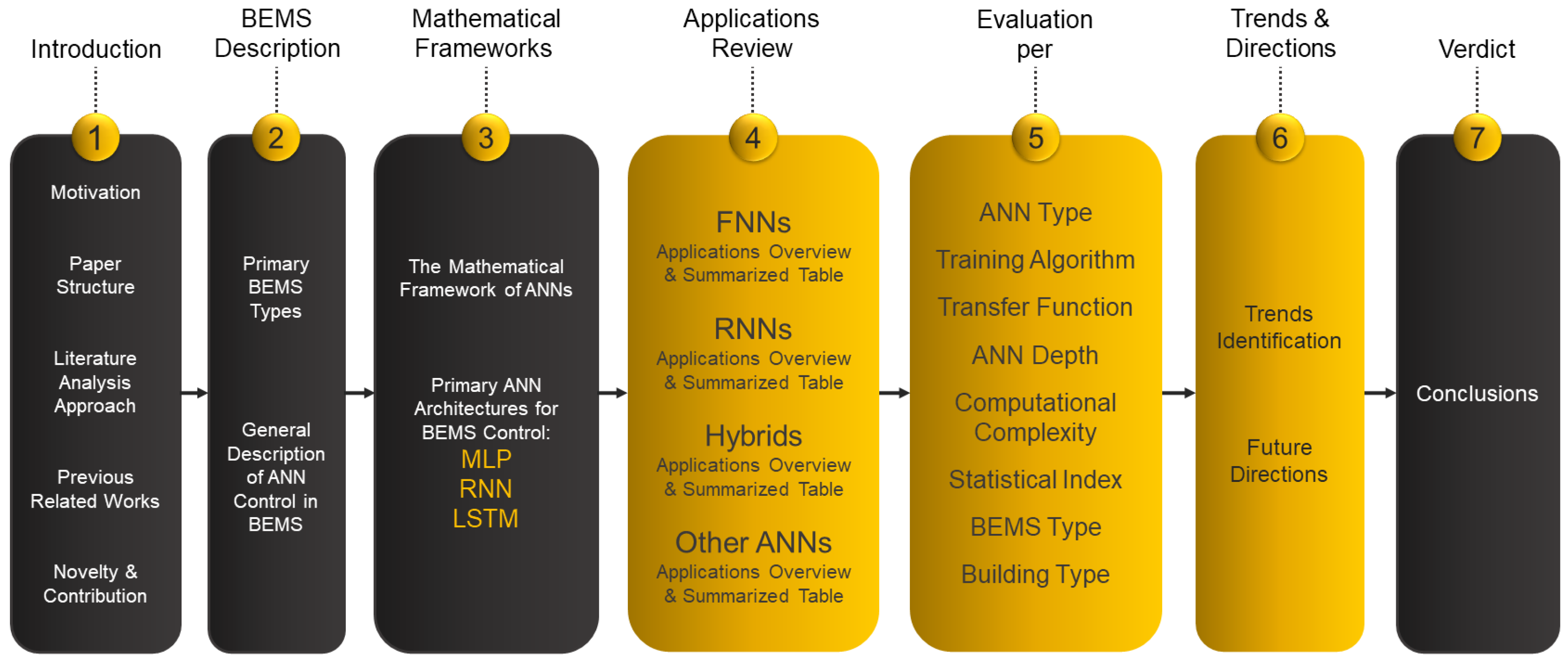


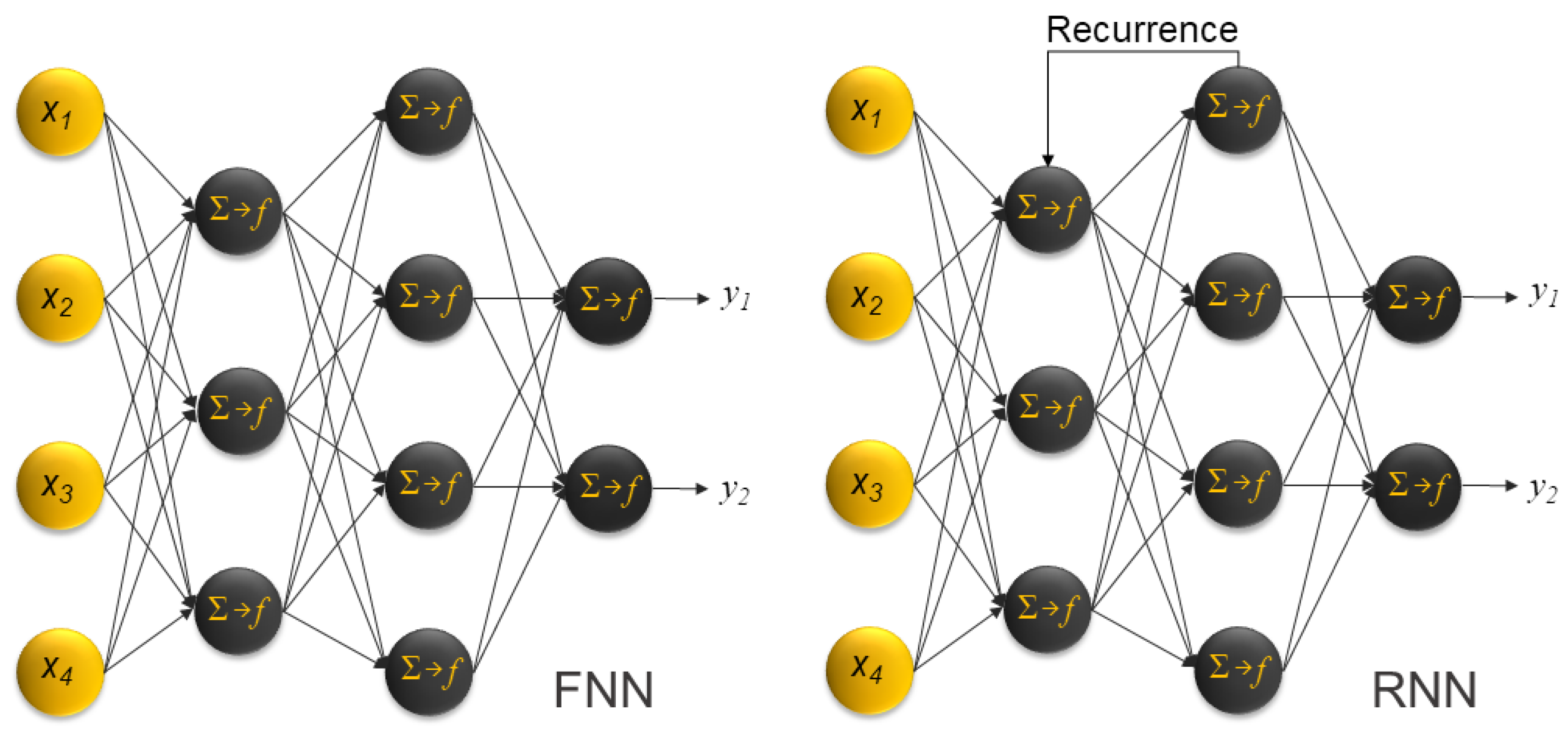
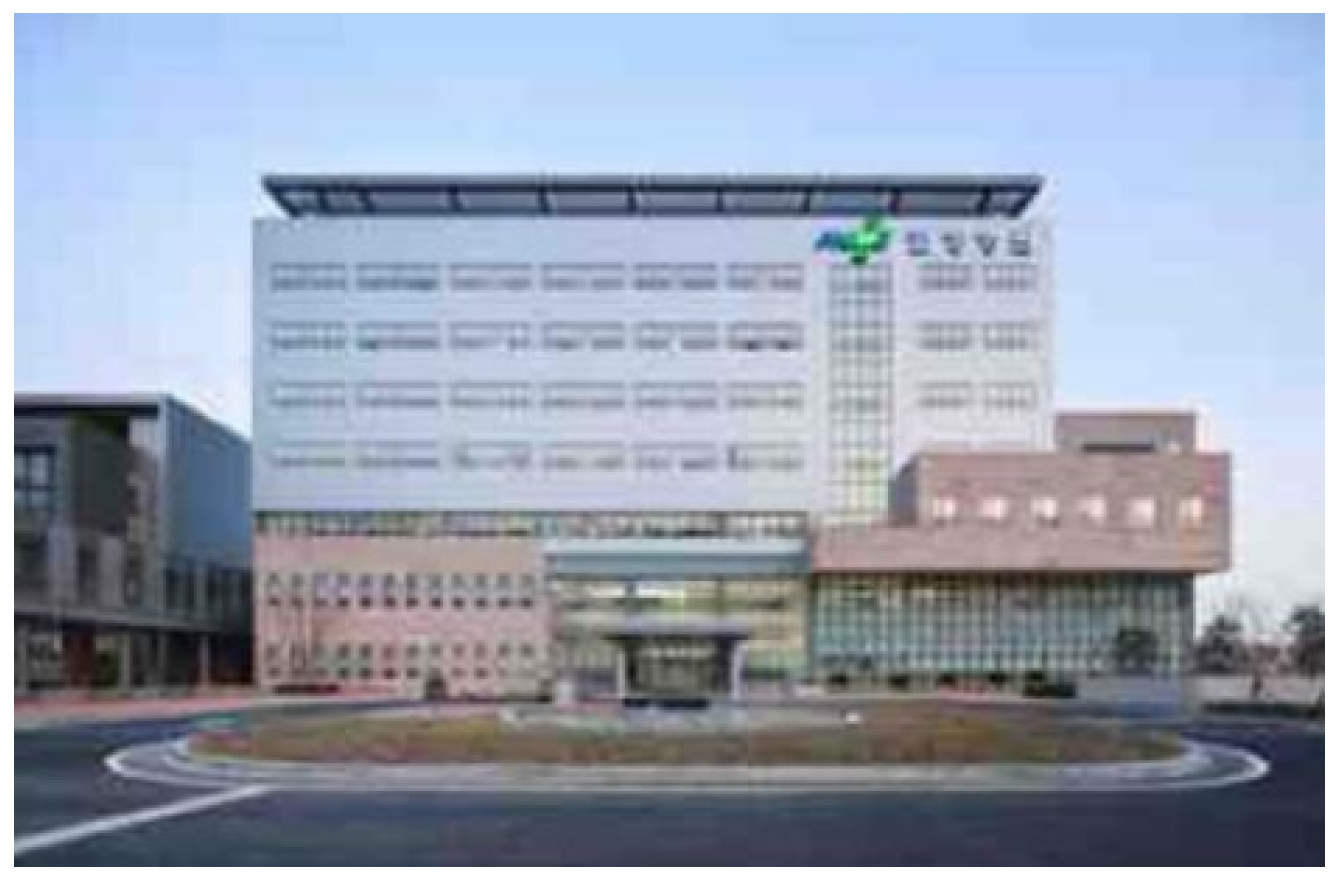
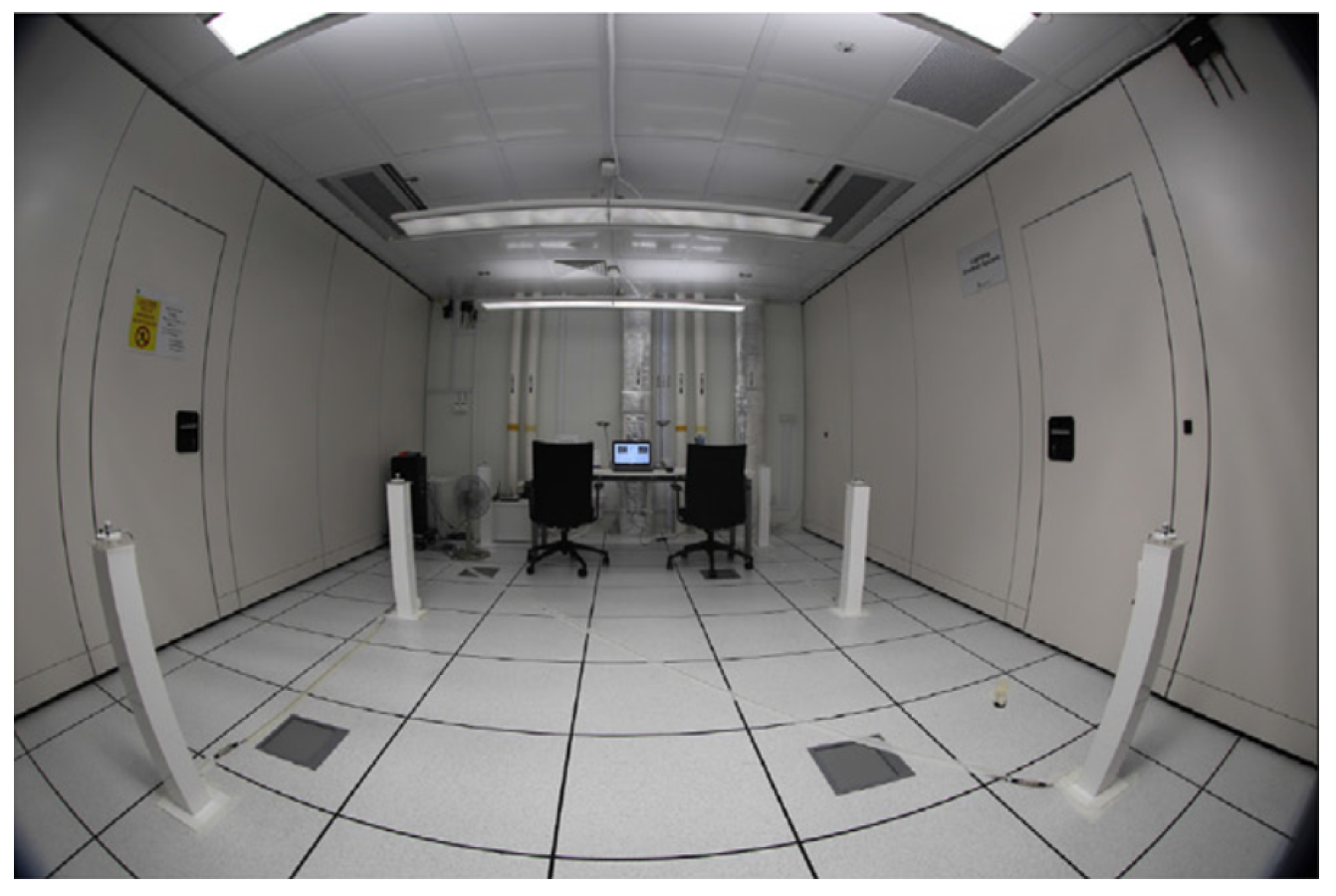
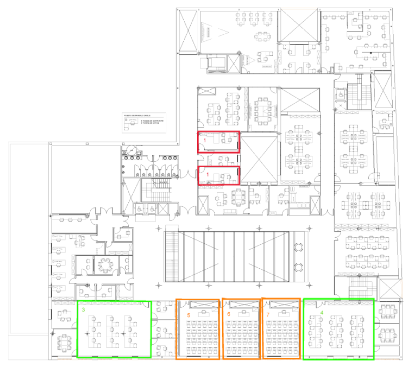
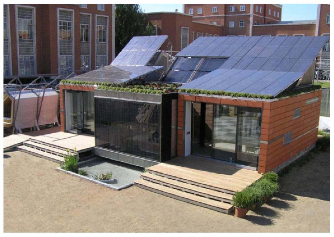
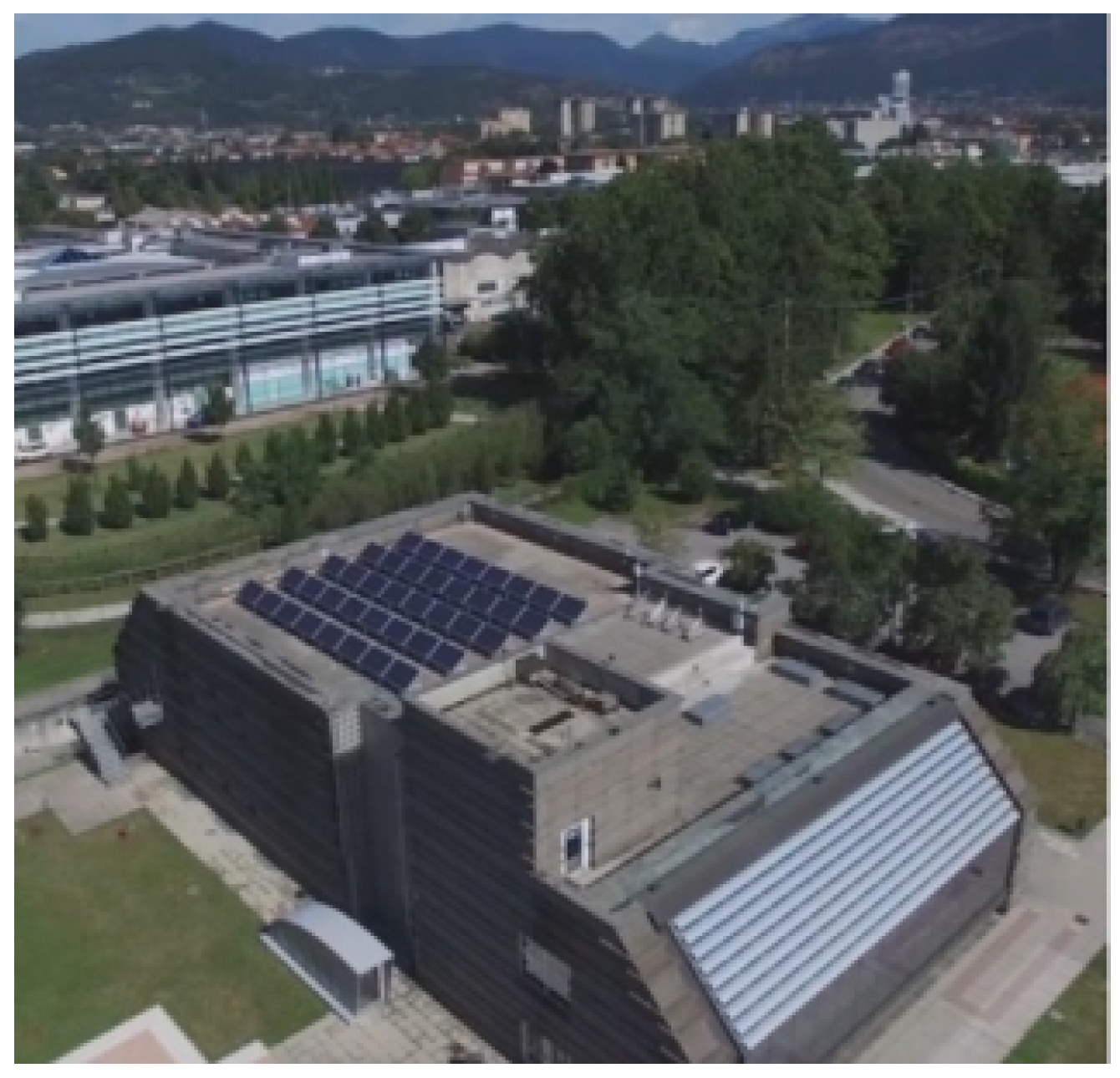
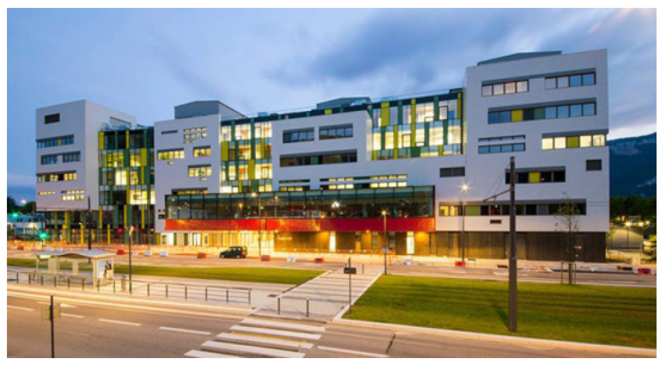
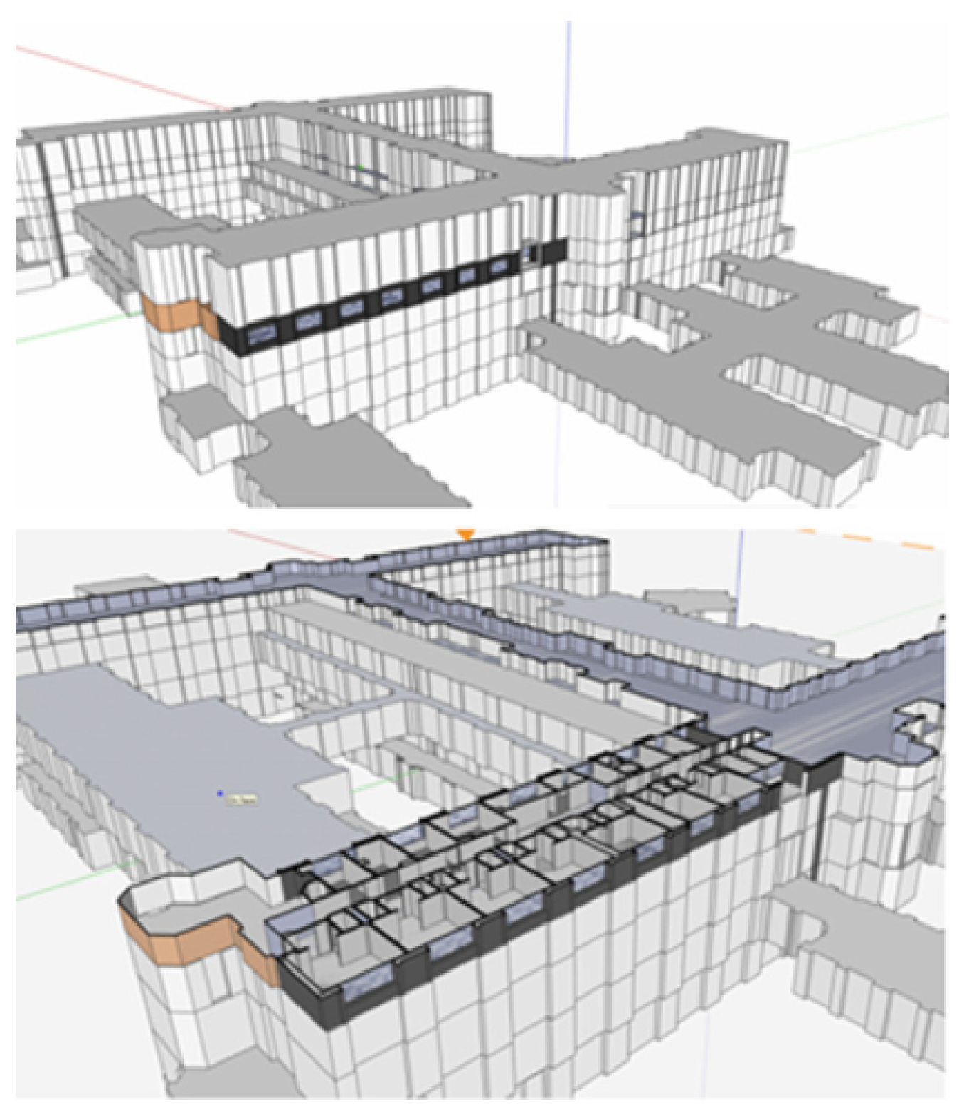

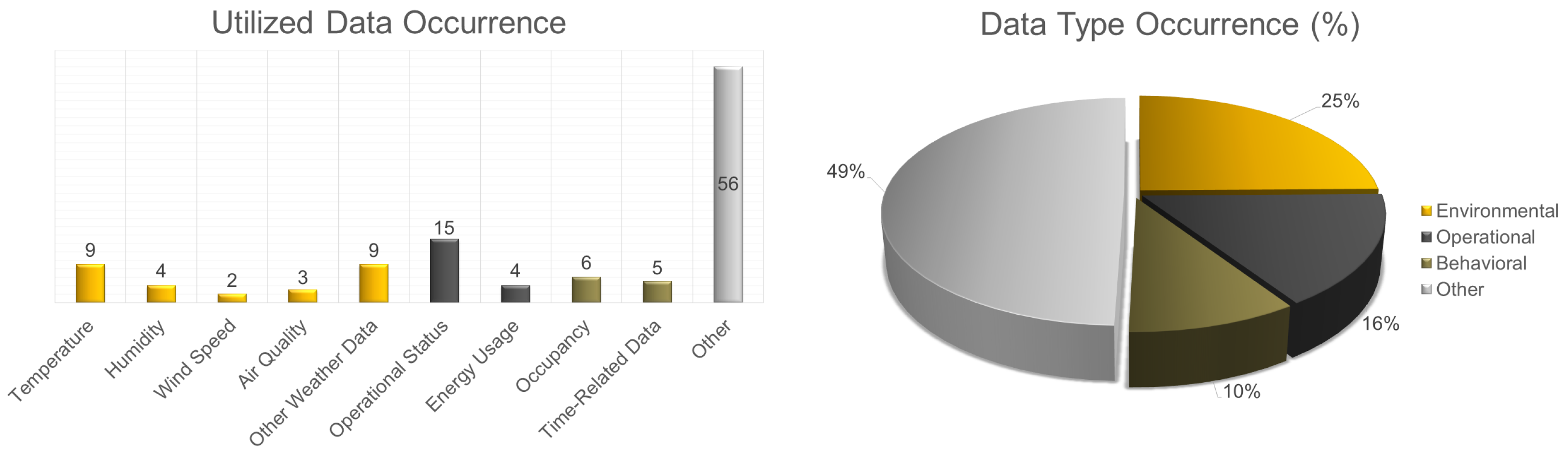

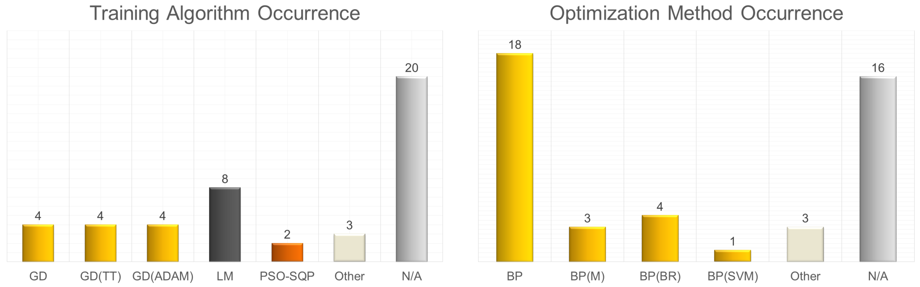
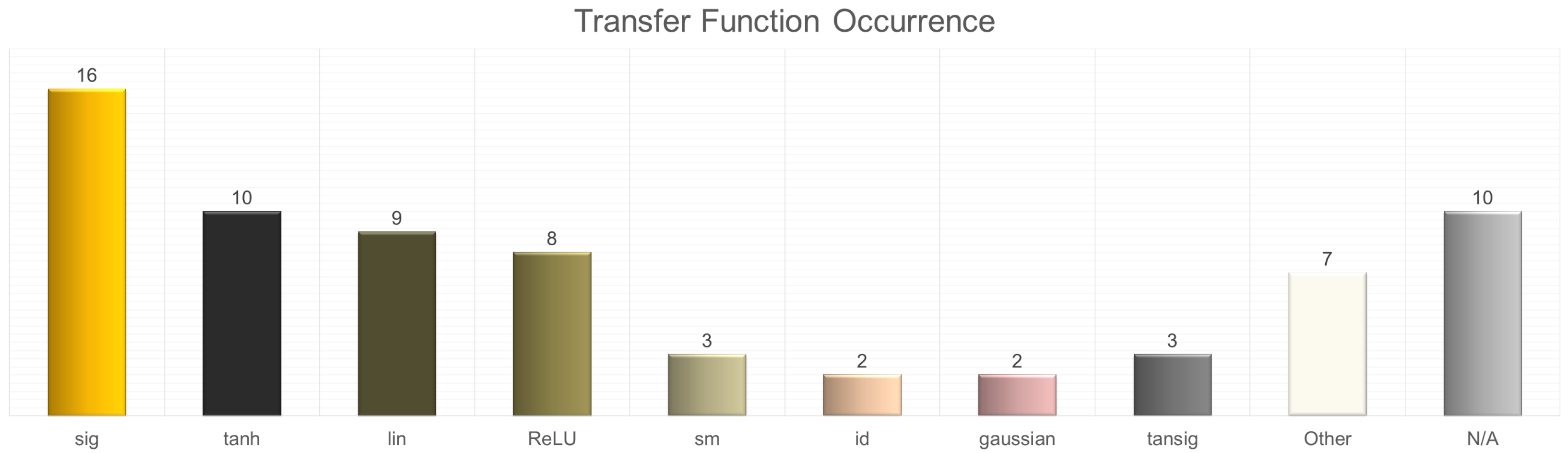

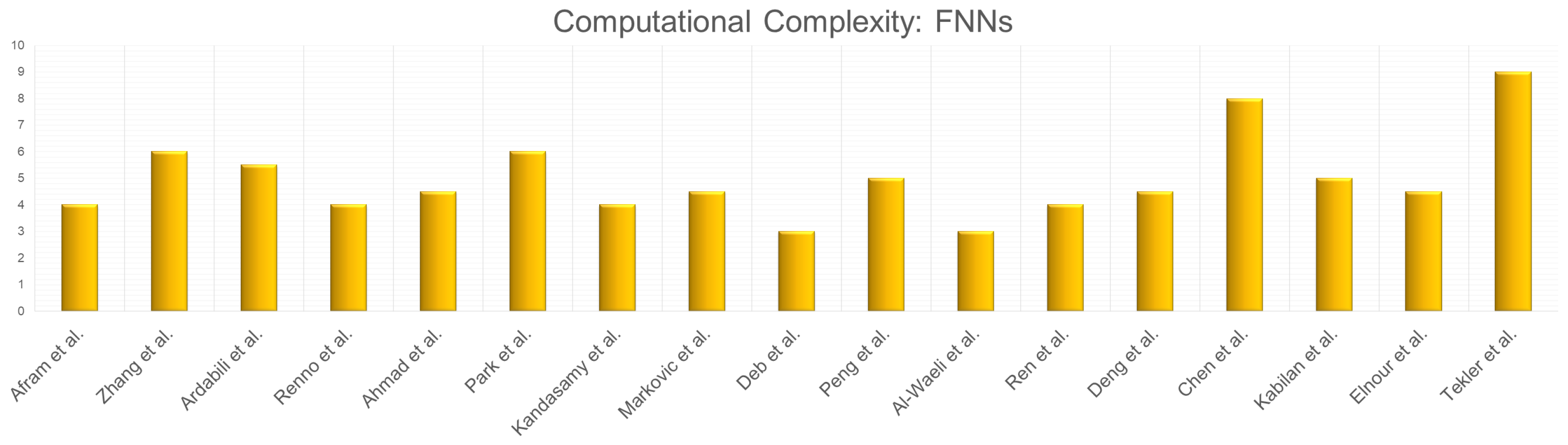
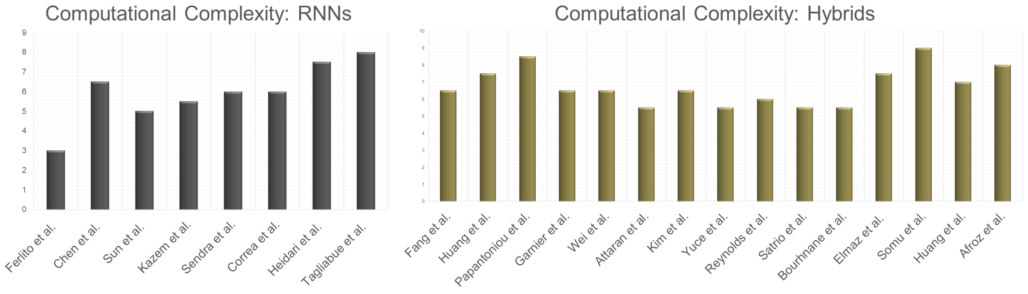
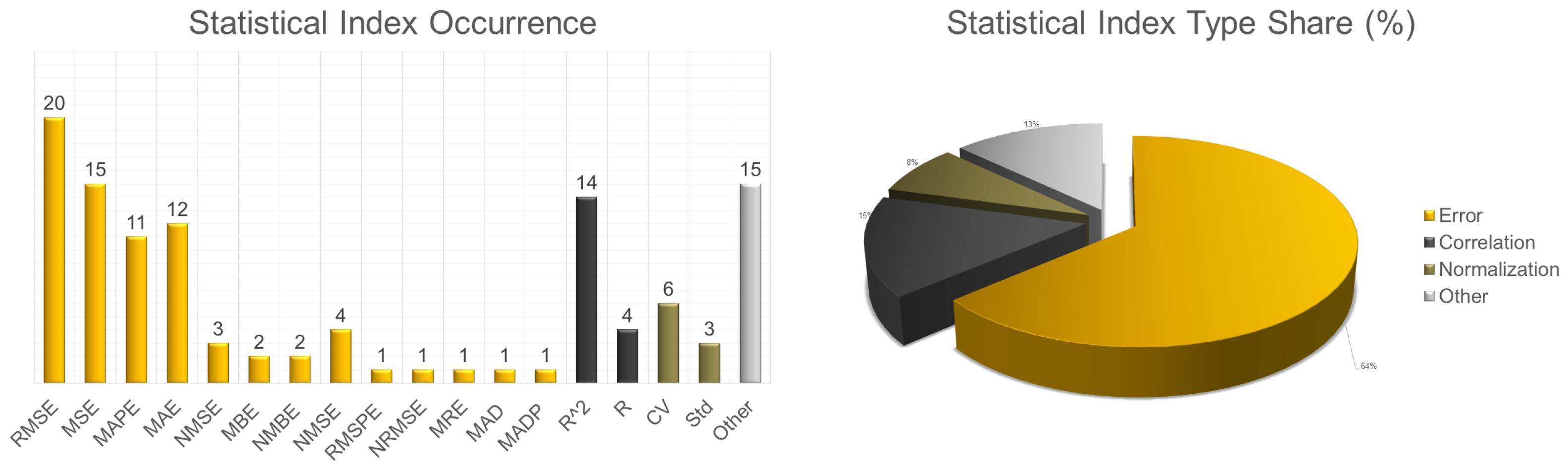


Disclaimer/Publisher’s Note: The statements, opinions and data contained in all publications are solely those of the individual author(s) and contributor(s) and not of MDPI and/or the editor(s). MDPI and/or the editor(s) disclaim responsibility for any injury to people or property resulting from any ideas, methods, instructions or products referred to in the content. |
© 2024 by the authors. Licensee MDPI, Basel, Switzerland. This article is an open access article distributed under the terms and conditions of the Creative Commons Attribution (CC BY) license (https://creativecommons.org/licenses/by/4.0/).