Article

Theoretical Study of Liquid Flow and Temperature Distribution in OF-Cooled Power Transformers

Kolektor Etra d.o.o, Šlandrova ulica 10, 1231 Ljubljana, Slovenia
*
Author to whom correspondence should be addressed.
Energies 2024, 17(3), 571; https://doi.org/10.3390/en17030571
Submission received: 20 December 2023 / Revised: 12 January 2024 / Accepted: 19 January 2024 / Published: 24 January 2024

Abstract

:
The objective of the paper is to analyse the effects of various geometrical and operating parameters on the liquid flow distribution in OF-cooled power transformers. Our investigation includes two cases: one with a simplified winding geometry and another that closely resembles the actual winding geometry. The analyses were carried out using computational fluid dynamics (CFD) and custom, internally developed thermo-hydraulic models. Our findings confirm that buoyancy forces rather than the pump drive the liquid flow within the windings of an OF-cooled power transformer. The results also show that the liquid flow distribution, which is influenced by the winding geometrical properties and liquid properties, has a significant impact on the hot-spot temperatures of the windings. The comparison between the results of the CFD simulations and the results of the simple model demonstrates a high level of agreement in calculating both the mass flow rates and temperatures.

1. Introduction

Like every other electrical device, a power transformer generates heat that needs to be effectively transferred to the environment. Therefore, every power transformer needs a cooling system. There are different cooling systems (cooling methods) defined by the IEC 60076-2 [1], which are typical for liquid-immersed power transformers. These cooling methods describe the circulation mechanism for the internal cooling medium (liquid) as well as the circulation mechanism and type of external cooling medium (water or air). The three methods of internal medium circulation are natural liquid flow (ON), directed forced liquid flow (OD), and forced liquid flow (OF). When an ester liquid is used, the letter “O” is substituted with the letter “K”.
Depending on the type of internal cooling mode, different liquid flow patterns emerge in the tank and in the active part (the windings and the magnetic core) of the transformer [2,3,4]. A schematic presentation of liquid flow distribution in a transformer is presented in Figure 1a. In the case of the OF cooling mode, the liquid flow is driven through the cooling equipment by a pump. No flow channels or barriers are used to direct the liquid flow into the windings. Therefore, it is expected that a part of the total liquid flow is flowing through the space between the tank and the windings (by-pass flow). In the case of the OF cooling mode, the flow through the windings, according to the IEC 60076-2 [1], is driven by the buoyancy forces (thermosiphon flow). Some other studies suggest that the liquid flow through the windings is primarily driven by the pump [5,6]. In general, there are very few studies investigating the internal liquid flow distribution in the case of the OF cooling mode. Such knowledge is important when designing an OF-cooled power transformer. Furthermore, understanding the liquid flow distribution between the active parts (windings and magnetic core) and the by-pass is crucial when developing thermo-hydraulic design tools, such as a thermo-hydraulic network model [6].
In the paper, we investigate how different parameters, such as the liquid mass flow rate, influence the liquid flow distribution in an OF-cooled power transformer. For the study, computational fluid dynamic (CFD) simulations considering a transformer with simplified winding geometries were carried out. Next, a mathematical model based on the principles of thermo-hydraulic network modelling [7,8] was developed for the simple geometry. The results of the mathematical model were compared to the results of the CFD simulations to evaluate the accuracy of the mathematical model. CFD simulations considering realistic winding geometries were carried out to validate the findings obtained from the simple geometry analyses. Again, a comparison between CFD simulation results and the results of a thermo-hydraulic network model was performed.

2. Liquid Flow and Temperature Distribution in OF-Cooled Power Transformers

In this section, the liquid flow and temperature distribution that is most likely to occur in an OF-cooled power transformer is described. The description is based on the information obtained from the literature [3,4,9,10] and based on in-house knowledge. Furthermore, the parameters under investigation, which are used in the following sections of the paper, are defined and described.
In Figure 1b, the temperature profiles over the height of the transformer are presented. One should be aware that in real situations, the temperature profiles are not linear; however, for the sake of explanation, a simplification considering linear profiles will suffice. It is expected that due to by-pass flow and variations in the hydraulic resistances of the windings, the temperature of the liquid in the windings will differ from the temperature of the liquid in the tank. Therefore, we define two different types of average liquid temperatures. The first average liquid temperature is the average liquid temperature in the tank, simply called the average liquid temperature ( θ om ). The average liquid temperature is defined as the average of the top-liquid temperature ( θ o ) and the bottom-liquid temperature ( θ b ). The second one is the winding average liquid temperature ( θ om , w ), which is defined as the average between the winding top-liquid temperature ( θ o , w ) and the bottom-liquid temperature ( θ b ). We also define two different winding gradients. The first one, denoted as “g”, is calculated as the temperature difference between the average winding temperature and the average liquid temperature. The second one, marked as “gw”, is calculated as the temperature difference between the average winding temperature and the average liquid temperature in the winding. In many cases, the average liquid temperature and the average winding liquid temperature are only slightly different. This might not always be the case, especially for OF-cooled transformers [1,4,5].

3. Simple Winding Geometry Simulations

Initially, a geometry with simplified windings was analysed. Simplifying the winding geometries significantly reduces the computational time required for CFD simulations. For the sake of simplicity, the magnetic core and insulation system (angle rings, static rings, etc.) above and below the windings were not considered in the simulations. Nevertheless, we took into account all the relevant physical phenomena occurring in a power transformer, and the results obtained from the simulations are expected to provide valuable insights and improve the understanding of the liquid flow patterns in OF-cooled transformers.

3.1. Case Description

A schematic presentation of the geometry under consideration can be seen in Figure 2. The geometry consists of two simple windings marked “winding 1” and “winding 2”. The windings are placed in a tank filled with liquid. Each winding has two vertical cooling channels. The width of the vertical cooling channels in “winding 1” (w1) is 2.5 times larger than the width of the vertical cooling channels in “winding 2” (w2). Such dimensions were selected to investigate how different hydraulic resistances of the cooling channels influence the liquid flow rate and temperatures of the windings. The windings were simulated as solid parts with uniform thermal conductivity. A constant volumetric heat generation of 118 kW m−3 was defined for both of the windings, which corresponds to approx. 5.4 kW of heat generation per winding. Such winding losses per winding phase are typical for power transformers in the range of around 5 MVA. The geometry under consideration also includes a simplified version of a heat exchanger. The heat exchanger geometry was selected in a way that the pressure drop in the heat exchanger corresponds to the values typically observed in compact heat exchangers of power transformers. A convective heat transfer boundary condition was defined for the external heat exchanger walls. The value of the heat transfer coefficient between the heat exchanger walls and the ambient was defined to achieve the desired temperature of the liquid exiting the heat exchanger. The coefficient ranged from 30 W m−2 K−1 to 45 W m−2 K−1. An ambient temperature of 301 K was considered for all the cases analysed because such a temperature is common during factory acceptance tests. Next, we assumed that the entire simple geometry exhibits an axial symmetry. The main dimensions of the geometry are given in Table 1. For the sake of simplicity, the winding cylinders and the tank walls were considered adiabatic.

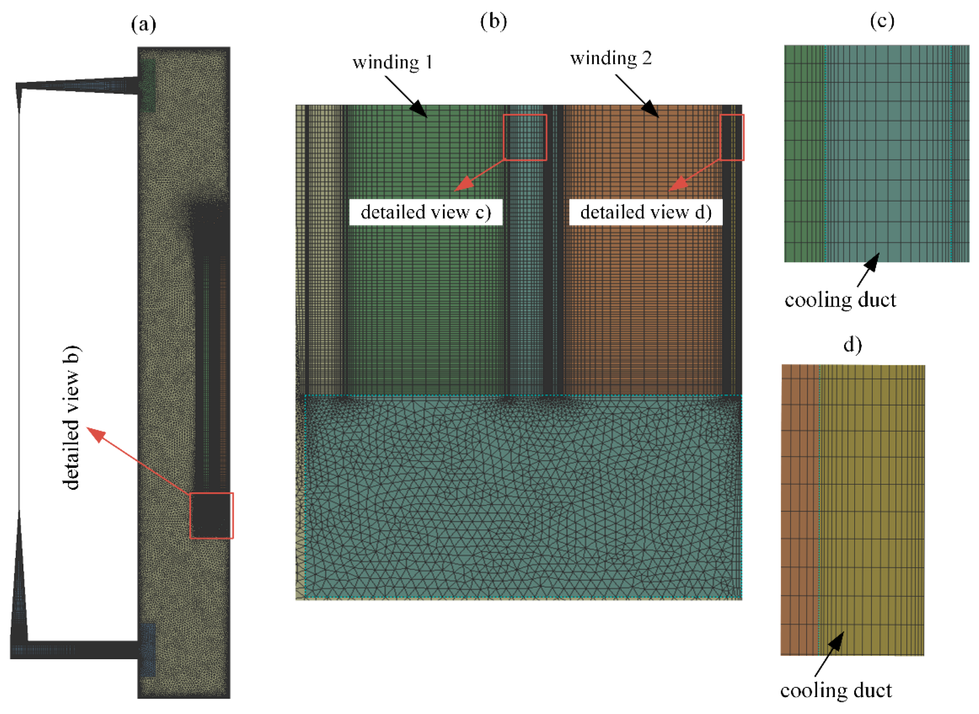
3.2. CFD Modelling and Solution Procedure

The CFD simulations were carried out using Ansys Fluent 2022 software, which gives numerical solutions to the conservation and transport equations. In this study, 2D axisymmetric simulations considering gravity were carried out. Energy and viscous (laminar) models were enabled for the simulations. The physical properties of the solid parts were assumed to be constant, while the properties of the liquid were considered to be temperature-dependent. The mesh of the simple model can be observed in Figure 3. The final 2D mesh consisted of 150,000 elements. Structured quadrilateral elements were used for the windings and the heat exchanger, while triangular elements were used to create the mesh of other parts. The mesh was refined near all the walls, especially in the windings (Figure 3c,d) and in the heat exchanger region to correctly capture the liquid temperature and velocity profiles. To check the mesh size independence, several sensitivity tests were carried out. All simulations were carried out in two steps. In the initial step, calculations were performed to obtain a steady-state solution. Since the convergence criteria for the steady-state simulations were not fully met, subsequent transient calculations were conducted. For the transient calculations, a fixed time step of 0.01 s was used. The convergence criteria for every time step were that the scaled residuals [11] for the continuity and velocity equations were smaller than 10−5, and for the energy equation, smaller than 10−6. The selected criterion for convergence is based on the values recommended in Ref. [11]. The transient calculations were continued until the main parameters under investigation reached a quasi-steady state. In this state, the parameters under investigation fluctuated around average values that remained constant over time.

3.3. Mathematical Model Based on the Thermo-Hydraulic Network Modelling Approach

Alongside the CFD simulations, the main parameters under investigation were calculated using a simple mathematical model. The simple model is based on the concept of thermo-hydraulic network modelling [7,8,12]. For the cases under investigation, we were mainly interested in how well the calculated liquid flow rate distribution matches the results of the CFD. First, the energy conservation equation for every liquid flow path can be written as follows:
Q i ˙ = m i ˙ · c p · T o u t , i T i n , i ,
where Q ˙ [W] is the heat flow rate, m ˙ [kg s−1] is the mass flow rate, c p [J kg−1 K−1] is the specific heat capacity of liquid, T o u t [K] is the liquid temperature exiting a winding or the by-pass and T i n [K] is the liquid temperature entering a winding or the by-pass. The index “i” denotes the individual flow paths. In total, there are three distinct flow paths in the system. The flow paths can be seen in Figure 2a, and they are marked with dashed blue lines. One flow path goes through the by-pass, while the other two flow paths pass through each of the windings. Next, we write the pressure change equations along each flow path:
Δ p i = ρ i · g · L i + f d · L i D h y , i · ρ i u i 2 2 ,
where Δ p i [Pa] is the pressure change, ρ [kg m−3] is the density, g [m s−2] is gravitational acceleration, L [m] is flow path length, f d [/] is the friction factor, D h y [m] is the hydraulic diameter and u [m s−1] is the velocity.
To calculate the friction factor, we use the correlation for a laminar flow between two parallel plates [13], which has the following form:
f D = 96 · ν u · D h y ,
where ν [m2 s−1] is kinematic viscosity. The hydraulic diameter for the case of laminar flow between two parallel plates accounts for 2 · w i . Next, we take into account that the pressure change along individual paths must be equal:
Δ p 1 = Δ p 2 = Δ p 3
Additionally, the liquid mass flow conservation must be respected:
m ˙ i = m ˙ t o t ,
where m ˙ t o t [kg s−1] is the total liquid mass flow entering the tank from the heat exchanger. Furthermore, we make the following assumptions:
  • The pressure drop due to hydraulic resistance of the by-pass flow path is much smaller than the pressure drop due to hydraulic resistance in the windings.
  • The temperature of the liquid above and below the windings is uniform.
  • The by-pass liquid temperature below the top of the windings equals the bottom-liquid temperature.
  • The liquid properties are determined based on average temperatures for every flow path.
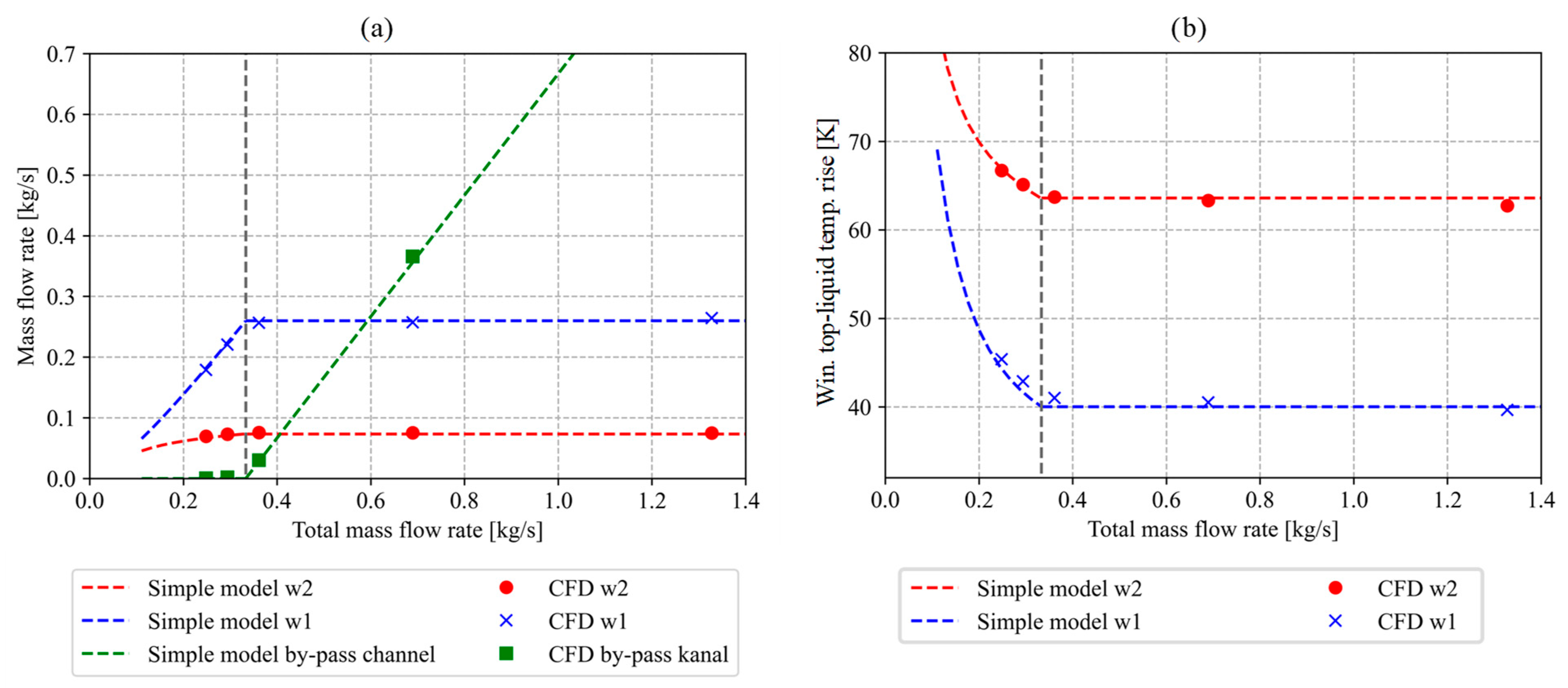
The solution procedure is as follows: first, we calculate the pressure change along the by-pass flow path using (2). Next, based on (1)–(4), we determine the mass flow rates through the windings. Now, the by-pass flow rate is calculated based on (5). In the following sections, we will find out that this approach has some limitations.

3.4. Results

Let us first analyse the results of a single CFD simulation to understand the basic characteristics of the temperature and the velocity field established in the tank and in the windings. The results under investigation correspond to a case in which the pump properties were set to produce a temperature difference of 8 K between the liquid entering the heat exchanger and the liquid exiting the heat exchanger. Such a temperature difference is typical for OF-cooled power transformers. The typical value is based on the in-house data for OF-cooled power transformers, and similar values are reported in the literature [5,6,14]. The total pump flow rate accounted for 0.58 kg s−1. The heat transfer coefficient between the heat exchanger wall and the ambient was set so that the temperature of the liquid exiting the heat exchanger (and entering the tank) accounted for 331 K. The ambient temperature of 301 K was considered for the study. The properties of the GTL liquid (gas-to-liquid) Diala S4 ZX-I [15,16], which were used for the simulations, are presented in Figure 4.
First, we neglected the heat generation in the windings. The simulation results are presented in Table 2 (“without heat generation”), where the mass flow rate through a winding is considered as the mass flow rate through the cooling channels (see also Figure 2b) of an individual winding. The results indicate that all the liquid flows through the by-pass. Such a result was expected due to a significant difference in the hydraulic resistance between the cooling channels of the windings and the by-pass. These initial simulation results already suggest that the pump is not driving the liquid flow through the windings. Instead, the presence of buoyancy forces is necessary to drive the liquid.
Next, heat generation in the windings was included in the simulation. The results of the simulation can be seen in Figure 5, where we can see the temperature and the velocity field for the case under investigation. From the temperature field presented in Figure 5a, we can see that different temperature zones are established. The liquid temperature in the space between the windings and the tank is constant from the bottom of the tank to the top of the windings. There, the cooler by-pass liquid flow mixes with the hotter liquid exiting the windings. Again, the temperature of the liquid in the space above the windings is quasi-uniform. Despite that, one can observe a region of hot liquid at the top of the tank. This phenomenon is caused by the hot liquid rising from the windings to the top of the tank. It is expected that the temperature of the hot liquid trapped below the top of the tank would be much closer to the liquid temperature entering the heat exchanger if the heat transfer from the tank to the ambient would be considered in the simulations.
Next, let us have a look at the main parameters under investigation, which are the liquid flow rates through the windings and the by-pass, as well as the tank top-liquid temperature (temperature of liquid entering the heat exchanger) and the winding top-liquid temperatures. The results for the cases analysed are presented in Table 2 and Table 3. We can observe a significant difference in mass flow rates between the two windings. The mass flow rate through “winding 2” (0.09 kg s−1) is more than three times smaller than the mass flow rate through “winding 1” (0.32 kg s−1). Such a result is no surprise since the width of the cooling channel of “winding 2” is much smaller than the width of the cooling channel of “winding 1”. Other parameters, such as heat generation and winding radius, are almost the same for the two windings. Therefore, their influence on the mass flow rates and temperatures is considered insignificant. Due to the relatively low mass flow rate through “winding 2” (inner winding), the winding top-liquid temperature rise of “winding 2” is 15.7 K higher than the winding top-liquid temperature rise of “winding 1” (outer winding) and 14.7 K higher than the liquid temperature at the heat exchanger inlet (top-liquid temperature rise).
Now, let us analyse the temperature gradients g and gw (as defined in Section 2). We can see that the winding duct gradient gw of “winding 2” is 4.3 K lower when compared to the winding duct gradient of “winding 1”. This discrepancy can be attributed to the fact that the narrower width of the cooling channel in “winding 2” facilitates more effective heat transfer between the winding and liquid in the winding duct. Contrary to the winding duct gradient (gw), the winding temperature gradient (g) of “winding 2” is greater than that of “winding 1”. This can be attributed to the fact that the average liquid temperature in “winding 2” is nearly 8 K higher compared to the average liquid temperature in “winding 1”. The impact of the higher winding liquid temperature becomes even more pronounced when examining the winding hot-spot temperatures. The high winding top-liquid temperature in “winding 2” results in a hot-spot temperature that is 9.6 K higher compared to “winding 1”. These observations show the importance of liquid flow distribution on the temperatures of the windings in the case of OF-cooled transformers.
Next, we analyse the influence of the total liquid mass flow rate on the main parameters under investigation. The simulations were carried out using the CFD model and the simple mathematical model presented in this paper. The mass flow rates considered in the study correspond to the temperature differences between the top-liquid temperature and the bottom-liquid temperature in the range from 2 K to 24 K. From here on, we will refer to these temperature differences as temperature drops. The properties of the heat exchanger were configured in a way that the bottom-liquid temperature remained constant. The results of the simulations are presented in Figure 6. In Figure 6a, we can see how the liquid mass flow rates along individual paths change as a function of the total liquid mass flow rate. At a reference temperature drop of 8 K, the total mass flow rate accounts for 0.58 kg s−1 (reference mass flow rate). As the mass flow rate is increased above the reference mass flow rate, one might expect that the mass flow rate through the windings will also increase. However, the simulation results indicate that both the mass flow rate and the temperature of the liquid exiting the windings remain constant. Only the by-pass mass flow rate increases when increasing the total mass flow rate to values higher than 0.58 kg s−1. On the other hand, as the total mass flow rate decreases to values lower than 0.58 kg s−1, there comes a point where the entire mass flow rate flows through the windings, and the by-pass mass flow rate decreases to zero. We will name this point the “transition point”. If the mass flow rate is further reduced from the “transition point” downward, the winding mass flow rates start decreasing. Consequently, the liquid temperatures exiting the windings start increasing. The “transition point” for the case under investigation corresponds to the mass flow rate of 0.43 kg s−1 and the temperature drop of around 10.5 K. At this point, we also need to describe an important limitation of the simple model. As the sum of the mass flow rates through the windings is approaching the total mass flow rate, the solution method, as presented in Section 3.3, is no longer functional because the method gives a negative by-pass mass flow rate. Therefore, as we reach the point of transition, the solution method and the model assumptions must change. We assume that the by-pass mass flow rate equals zero. Therefore, Equations (1)–(5) are solved for the two windings paths only.
A comparison between the results of the CFD simulation and the results of the simple mathematical model shows that the simple model accurately predicts the results obtained using CFD. For example, the deviations between the mass flow rates calculated with the CFD and calculated with a simple model are no larger than 5% for both of the windings and for the by-pass flow. To put it differently, the winding top-liquid temperatures calculated using CFD differ from the winding top-liquid temperatures calculated using the simple model for no more than 1 K.
The simulations were also carried out for a case in which the properties of a synthetic ester, Midel 7131 [17], are defined as the liquid properties. The results of the simulations are presented in Figure 7. Again, the deviations between the mass flow rates calculated using the CFD model, and the simple model are no larger than 5%.
Next, the results of simulations considering GTL liquid and synthetic ester are compared. A shift in the transition point from 0.43 kg s−1 in the case of GTL liquid to 0.33 kg s−1 in the case of synthetic ester can be observed. This shift can be attributed to the higher viscosity of synthetic ester. With higher viscosity, the hydraulic resistances of the windings increase; therefore, the buoyancy forces drive less liquid through the windings, and the transition point shifts to lower values. It can also be observed that in the case of synthetic ester, the mass flow rates through the windings (for cases in which the total mass flow rate is beyond the transition point) are 20% lower for “winding 1” and 25% lower for “winding 2”. This results in a winding top-liquid temperature that is 5 K higher for “winding 2” and 10 K higher for “winding 1”. In conclusion, the higher the viscosity of the liquid, the higher the winding top-liquid temperature and the higher the deviation between the top-liquid temperature in the tank and the top-liquid temperature in the windings.

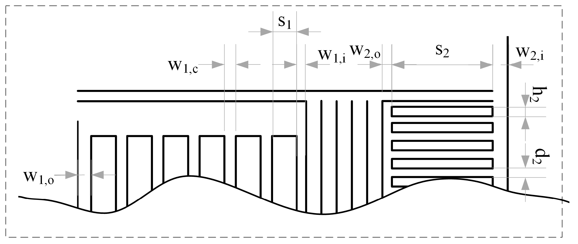
4. Complex Winding Geometry

To validate the findings obtained from the results of the simplified winding model, we conducted additional simulations using a more realistic representation of the windings.

Case and Calculation Description

For cases involving complex winding geometry, the overall geometry layout of the complete system (tank + heat exchanger + windings) remained unchanged, and it is schematically presented in Figure 2a. However, the dimensions indicated in Figure 2a were adjusted to more closely represent a real-word transformer. Furthermore, the winding details no longer correspond to those presented in Figure 2b but are now different and can be seen in Figure 8. All dimensions for the case with complex windings are given in Table 4. The “winding 1” has seven vertical cooling channels and no radial channels. On the other hand, “winding 2” has two vertical cooling channels and radial channels between the winding discs. Additionally, “winding 2” has liquid-guiding elements, which are used to guide the liquid flow through radial channels. The geometries of the windings were intentionally selected to exhibit a significant difference in hydraulic resistance between them. This design choice was made to emphasize the impact of hydraulic resistance on the liquid flow distribution. We defined a constant volumetric heat generation of 42.6 kW m−3 for “winding 1” and a constant volumetric heat generation of 127.0 kW m−3 for “winding 2”.
First, we carried out CFD simulations. The solution procedure remained the same as described in Section 3.2. However, when compared to the simple case, the winding cylinders and other auxiliary winding structures were not considered adiabatic. Again, the ambient temperature was set to 301 K, and the heat transfer coefficient between the heat exchanger and the ambient was set so that the temperature of the liquid exiting the heat exchanger accounted for 331 K. The pressure change of the pump was set to produce an 8 K temperature difference between the liquid entering and exiting the heat exchanger. Two cases were analysed: in the first case, the properties of the GTL liquid were considered, while in the second case, the properties of the synthetic ester were taken into account.
In addition to the CFD results, a thermo-hydraulic network model was used to simulate the same case. The modelling technique is similar to the mathematical model presented in Section 3.3. However, to model the complex winding geometry, the level of detail is higher. To find out more about thermo-hydraulic network models, the reader is referred to Refs. [6,7,18]. Just as in the case of the simple mathematical model, we formulate certain modelling assumptions. These assumptions mirror those specified as assumptions (1), (2) and (3) of the simple model. Furthermore, we introduce some additional assumptions:
  • The heat transfer coefficient in the cooling channels of the windings is calculated using equations for the Nusselt number, which are valid for laminar flow between parallel plates with constant heat flux. The equations can be found in Ref. [13].
  • The pressure drop coefficient is calculated using equations valid for hydraulically developing laminar flow between parallel plates. The equations can be found in Ref. [13].
  • Local pressure drops in the windings and in the insulation system below and above the windings are neglected.
In Figure 9, the temperature and the velocity field of the complex winding geometry are presented. We can observe the establishment of temperature zones, which are very similar to the case of the simple winding geometry. However, one can notice that there is a difference in the intensity of the mixing of the liquid above the windings and that the temperature is not as uniform as in the case of simple windings.
The main parameters under investigation, calculated using the CFD and thermo-hydraulic network model (THN model), are presented in Table 5. From the results, we can observe that the winding top-liquid temperature rise in “winding 2” (in the case of GTL liquid), calculated using CFD, is 14.1 K higher than the tank top-liquid temperature rise. The difference is even higher for the synthetic ester and accounts for 23.6 K. On the other hand, the winding top-liquid temperature rise for “winding 1” is more or less the same as the tank top-liquid temperature rise. Next, we observe that the winding duct gradient of “winding 2” (2.7 K) is smaller than the winding duct gradient of “winding 1” (4.9 K). On the contrary, when comparing the hot-spot temperatures, we can see that the hot-spot temperature of “winding 2” is 11.8 K higher than the hot-spot temperature of “winding 1” (using GTL liquid). The findings show that in the case investigated, the winding top-liquid temperature has the greatest impact on the magnitude of the winding hot-spot. The same conclusions can be made for the simulation case with synthetic ester; this time, the winding top-liquid temperature has an even larger impact on the winding hot-spot. These results highlight the importance of understanding and accurately predicting the winding liquid temperatures, which are directly influenced by the liquid flow distribution between the liquid flow paths.
When comparing the results of the CFD simulation to the results of the THN model, we can observe that the differences in the calculated temperatures are no more than a few K. These results provide us with confidence that the thermo-hydraulic network modelling technique captures all the significant phenomena influencing the liquid flow distribution and temperatures in OF-cooled power transformers.

5. Conclusions

In the paper, we theoretically investigated the influence of various parameters on the liquid flow and temperature distribution in OF-cooled power transformers. Different winding geometries, various operating conditions and three theoretical models with different levels of modelling detail were used in the study. The study considers and compares two types of liquids: a GTL and a synthetic ester.
The results of the CFD simulations show that in the case of OF cooling mode, buoyancy forces are necessary to establish the liquid flow through the windings. This was first revealed through CFD simulations for the simple case with heat generation in the windings neglected, which showed that the liquid flow in the windings is not established.
The simulation results of the simple winding case indicate the presence of a “transition point”, characterized by a specific mass flow rate. An increase in the total mass flow beyond the “transition point” does not result in a corresponding increase in the mass flow rate through the windings. Instead, only the by-pass mass flow rate is increased. However, one should avoid decreasing the total mass flow rate below the transition point since this will cause higher liquid and winding temperatures. We can conclude that for the case under investigation, the pump does not have a direct influence on the liquid flow rate through the windings.
In both cases under investigation (the simple and the complex winding geometry), our observations reveal that the critical factor influencing the magnitude of the winding hot-spot is not the winding duct temperature gradient (the difference between the average winding temperature and the average winding liquid temperature). Instead, the winding top-liquid temperature was the main factor that determined the magnitude of the winding hot-spot. The results of the simulations show that the winding top-liquid temperature can be substantially higher for winding geometries with narrower cooling ducts. Furthermore, considering a liquid with a higher viscosity (using the synthetic ester instead of the GTL liquid) also results in an increase in the winding top-liquid temperature and, consequently, in an increase in the winding hot-spot temperatures. On the one hand, accurate design tools are needed to correctly predict such behaviour, and on the other side, good design practices should be used to avoid scenarios in which the winding top-liquid temperatures are substantially higher than tank top-liquid temperatures.
The comparison between the results of the CFD simulations and the results of the simple model demonstrates a high level of agreement in calculating the mass flow rates and temperatures. Even for the more complex winding geometry, small deviations were observed between parameters calculated using CFD and THN models. One should be careful not to generalize these findings. In different scenarios, such as when considering the core and heat transfer to the environment or altering operating conditions, the deviations between the CFD and THN models presented in this study might vary. Next, only a comparison with experimental results would reveal the accuracy of these models in predicting ‘real-world’ scenarios. For predicting liquid flow distribution and temperatures in real-world scenarios, the simple mathematical model would probably lack some degree of detail, especially when predicting hot-spots of windings with complex geometries. The comparison of theoretical models with experimental results is beyond the scope of this paper and is reserved for future work. However, the small deviations between the CFD and THN models obtained in this study suggest that the thermo-hydraulic models can capture the most significant phenomena that influence the liquid flow and liquid temperature distribution in OF-cooled power transformers.

Author Contributions

Conceptualization, U.P., B.B. and B.P.; methodology, U.P., B.B. and B.P.; formal analysis, U.P. and B.B.; investigation, U.P. and B.B.; writing—original draft preparation, U.P.; review and editing, U.P., B.B. and B.P.; visualization, U.P. and B.B.; supervision, B.P. All authors have read and agreed to the published version of the manuscript.

Funding

This research received no external funding.

Data Availability Statement

Data are contained within the article.

Conflicts of Interest

Authors U.P., B.B. and B.P. were employed by the company Kolektor Etra d.o.o.

References

  1. IEC 60076-2:2011; Power Transformers—Part 2: Temperature Rise for Liquid-Immersed Transformers. IEC: Geneva, Switzerland, 2011.
  2. Yamaguchi, M.; Kumasaka, T.; Inui, Y.; Ono, S. The flow rate in a self-cooled transformer. IEEE Trans. Power Appar. Syst. 1981, PAS-100, 956–963. [Google Scholar] [CrossRef]
  3. Karsai, K.; Kerényi, D.; Kiss, L. Large Power Transformers; Elsevier: Amsterdam, The Netherlands, 1987. [Google Scholar]
  4. Sorgic, M.; Radakovic, Z. Oil-Forced Versus Oil-Directed Cooling of Power Transformers. IEEE Trans. Power Deliv. 2010, 25, 2590–2598. [Google Scholar] [CrossRef]
  5. Godec, Z.; Šarunac, R. Steady-state temperature rises of ONAN/ONAF/OFAF transformers. IEE Proc. C Gener. Transm. Distrib. 1992, 139, 448–454. [Google Scholar] [CrossRef]
  6. Convenor, J.L. Transformer Thermal Modelling; Working Group A2.38; CIGRE Publication: Paris, France, 2016. [Google Scholar]
  7. Radakovic, Z.R.; Sorgic, M.S. Basics of Detailed Thermal-Hydraulic Model for Thermal Design of Oil Power Transformers. IEEE Trans. Power Deliv. 2010, 25, 790–802. [Google Scholar] [CrossRef]
  8. Zhang, J.; Li, X. Analysis for Oil Thermosyphon Circulation and Winding Temperature in ON Transformers. In Proceedings of the 2007 IEEE Power Engineering Society General Meeting, Tampa, FL, USA, 24–28 June 2007; pp. 1–8. [Google Scholar]
  9. IEC 60076-7:2018; Power Transformers—Part 7: Loading Guide for Mineral-Oil-Immersed Power Transformers. IEC Standard: Geneva, Switzerland, 2018.
  10. Vecchio, R.M.D.; Poulin, B.; Feghali, P.T.; Shah, D.M.; Ahuja, R. Transformer Design Principles: With Applications to Core-Form Power Transformers; CRC Press/Taylor & Francis Group: London, UK, 2001. [Google Scholar]
  11. ANSYS. Fluent User’s Guide Release 2022 R1 January 2022; ANSYS Inc.: Canonsburg, PA, USA, 2022. [Google Scholar]
  12. Oliver, A. Estimation of transformer winding temperatures and coolant flows using a general network method. IEE Proc. C Gener. Transm. Distrib. 1980, 127, 395–405. [Google Scholar] [CrossRef]
  13. Shah, R.K.; London, A.L. Laminar Flow Forced Convection in Ducts: A Source Book for Compact Heat Exchanger Analytical Data; Academic Press: New York, NY, USA, 1978. [Google Scholar]
  14. Susa, D.; Lehtonen, M.; Nordman, H. Dynamic Thermal Modelling of Power Transformers. IEEE Trans. Power Deliv. 2005, 20, 197–204. [Google Scholar] [CrossRef]
  15. Zhang, X.; Wang, Z.; Lui, Q.; Jarman, P.; Gyore, A.; Dyer, P. Numerical Investigation of Influences of Coolant Types on Flow Distribution and Pressure Drop in Disc Type Transformer Windings. In Proceedings of the International Conference on Condition Monitoring and Diagnosis CMD, Xi’an, China, 25–28 September 2016; pp. 52–55. [Google Scholar] [CrossRef]
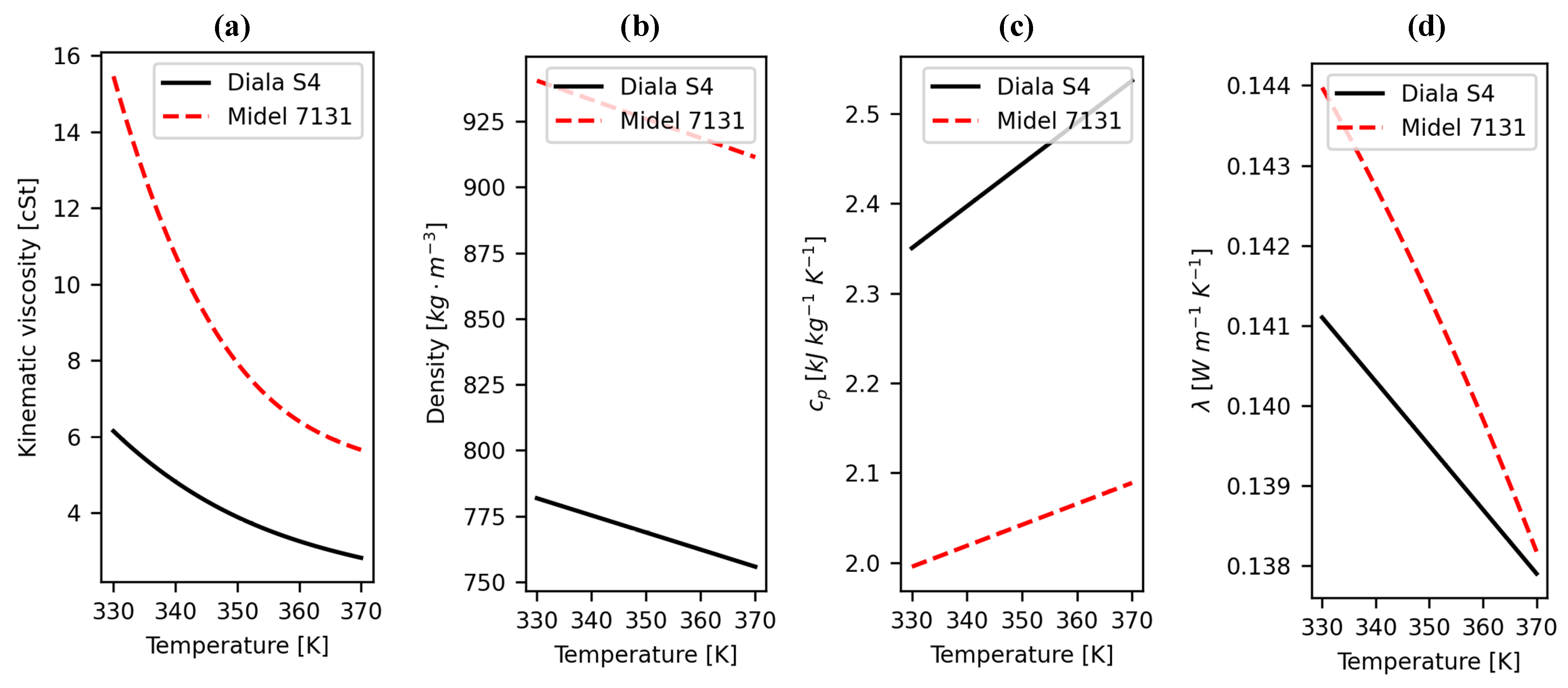
  16. Daghrah, M.; Wang, Z.; Liu, Q.; Hilker, A.; Gyore A., A. Experimental Study of the Influence of Different Liquids on the Transformer Cooling Performance. IEEE Trans. Power Deliv. 2019, 34, 588–595. [Google Scholar] [CrossRef]
  17. Midel 7131: Thermal Properties. Available online: https://www.midel.com/app/uploads/2018/09/MIDEL_7131_Thermal_Properties.pdf (accessed on 18 December 2023).
  18. Plaznik, U.; Klobučar, L.; Prašnikar, B. Thermal design of ester filled power transformers. In Proceedings of the 41. CIGRE International Symposium, Ljubljana, Slovenia, 21–24 November 2021; p. 1194. [Google Scholar]
Figure 1. (a) Schematic presentation of liquid flow distribution in case of OF cooling mode. (b) Diagram showing simplified liquid and winding temperature profiles along the height of a power transformer.
Energies 17 00571 g001
Figure 2. Simple case. (a) Schematic presentation of the geometry under consideration. (b) Detailed view of the windings.
Energies 17 00571 g002
Figure 3. Mesh of the simple geometry. (a) Complete geometry. (b) Detailed view of the bottom of the windings. (c) Detailed view of the inner cooling duct of “winding 1”. (d) Detailed view of the inner cooling duct of “winding 2”.
Energies 17 00571 g003
Figure 4. Liquid properties of Diala S4 ZX-I and Midel 7131. The properties are shown in the range of temperatures relevant to the simulations. (a) Kinematic viscosity. (b) Density. (c) Specific heat capacity. (d) Thermal conductivity.
Energies 17 00571 g004
Figure 5. CFD results for simple winding geometry considering GTL liquid. (a) Temperature field. (b) Velocity field.
Energies 17 00571 g005
Figure 6. (a) Liquid mass flow rate through the individual flow paths as a function of the total liquid mass flow rate. (b) Winding top-liquid temperatures rise over the ambient. Both figures present the results of simulations considering GTL liquid.
Energies 17 00571 g006
Figure 7. (a) Liquid mass flow rate through the individual flow paths as a function of the total liquid mass flow rate. (b) Winding top-liquid temperatures rise over the ambient. Both figures present results of simulations considering synthetic ester.
Energies 17 00571 g007
Figure 8. Details of complex winding geometry.
Energies 17 00571 g008
Figure 9. CFD results for complex winding geometry considering GTL liquid. (a) Temperature field. (b) Velocity field.
Energies 17 00571 g009
Table 1. Geometrical properties for the simple case.
SymbolBCHLHXLwr1r2s1s2wHXw1w2
Value [mm]303.550.01100.0667.0493.1668.5694.021.221.21.35.02.0
Table 2. Mass flow rate through different parts of the transformer for two scenarios: without heat generation and with heat generation in the windings.
m ˙ [kg s−1]
By-PassWind. 1Wind. 2
Without heat generation0.580.00.0
With heat generation0.170.320.09
Table 3. Results of simulations considering simple winding geometry.
DescriptionSymbolCFDSimple Model
Top-liquid temperature rise [K] Δ θ o 38.038.0
Average liquid temperature rise [K] Δ θ om 34.034.0
Winding 1212
Wind. top-liquid temperature rise [K] Δ θ o , w 37.052.736.453.0
Wind. average liquid temperature rise [K] Δ θ om , w 33.541.433.241.5
Winding duct gradient [K]gw12.3 8.0//
Winding gradient [K]g11.815.4//
Average wind. temperature rise [K] Δ θ w 45.849.4//
Hot-spot temperature rise [K] Δ θ h 50.960.5//
Hot-spot factor [/]H1.091.46//
Table 4. Geometrical properties of the complex windings. Please refer to Figure 2a and to Figure 8 to identify the meaning of the symbols used in the table.
SymbolBd2h2HLHXLw,1Lw,2r1r2s1s2wHXw1,ow1,cw1,iw2,ow2,i
Value [mm]0.929330020001480154055641821.2781.2565676
Table 5. Results of simulations considering complex winding geometry.
DescriptionSymbolCFDTHN Model
Top-liquid temperature rise [K] Δ θ o 38.038.0
Average liquid temperature rise [K] Δ θ om 34.034.0
Liquid type GTLSyn. esterGTLSyn. ester
Winding 12121212
Wind. top-liquid temperature rise [K] Δ θ o , w 37.752.141.461.639.054.042.864.1
Wind. average liquid temperature rise [K] Δ θ om , w 33.941.135.745.834.542.036.447.4
Winding duct gradient [K]gw4.92.75.12.84.52.24.92.0
Winding gradient [K]g4.89.86.814.65.010.27.315.4
Average wind. temperature rise [K] Δ θ w 38.843.840.848.639.044.241.349.4
Hot-spot temperature rise [K] Δ θ h 43.855.647.965.343.056.047.066.0
Hot-spot factor [/]H1.21.81.51.91.01.81.21.8
Disclaimer/Publisher’s Note: The statements, opinions and data contained in all publications are solely those of the individual author(s) and contributor(s) and not of MDPI and/or the editor(s). MDPI and/or the editor(s) disclaim responsibility for any injury to people or property resulting from any ideas, methods, instructions or products referred to in the content.

