A Machine Learning-Based Electricity Consumption Forecast and Management System for Renewable Energy Communities

Abstract

The energy sector is currently undergoing a significant shift, driven by the growing integration of renewable energy sources and the decentralization of electricity markets, which are now extending into local communities. This transformation highlights the pivotal role of prosumers within these markets, and as a result, the concept of Renewable Energy Communities is gaining traction, empowering their members to curtail reliance on non-renewable energy sources by facilitating local energy generation, storage, and exchange. Also in a community, management efficiency depends on being able to predict future consumption to make decisions regarding the purchase, sale and storage of electricity, which is why forecasting the consumption of community members is extremely important. This study presents an innovative approach to manage community energy balance, relying on Machine Learning (ML) techniques, namely eXtreme Gradient Boosting (XGBoost), to forecast electricity consumption. Subsequently, a decision algorithm is employed for energy trading with the public grid, based on solar production and energy consumption forecasts, storage levels and market electricity prices. The outcomes of the simulated model demonstrate the efficacy of incorporating these techniques, since the system showcases the potential to reduce both the community electricity expenses and its dependence on energy from the centralized distribution grid. ML-based techniques allowed better results specially for bi-hourly tariffs and high storage capacity scenarios with community bill reductions of 9.8%, 2.8% and 5.4% for high, low, and average photovoltaic (PV) generation levels, respectively.

1. Introduction

Energy systems are changing at a rapid pace, driven by the imperative to diminish reliance on non-renewable resources. The increase in the renewable energy penetration rate brings environmental and economic benefits to the power system; however, it also poses challenges to load dispatch and energy management mechanisms [1]. Novel control approaches are thus being proposed to integrate renewable electricity sources, like photovoltaic (PV) panels and wind turbines, as well as new power loads, such as electric vehicles (EVs), in the context of microgrid systems [2].

This energy transformation is paving the way for the emergence of a novel market paradigm centered around prosumers: individuals or institutions who not only consume energy, but also possess the capacity to generate and store electricity. A recent development in electricity markets involves the design and implementation of peer-to-peer (P2P) architectures, enabling prosumers to directly exchange electricity among them [3]. These P2P markets adopt a grassroots approach in a local context, empowering prosumers to collectively manage energy operations under the scope of Renewable Energy Communities (RECs). Within RECs, all participants (prosumers) collaborate using their available resources to create, trade, or distribute assets and services based on cooperative principles, streamlining transactions among all economic agents [4]. This way, REC members can better adjust their energy consumption preferences, including a penchant for renewable energy sources, a drive to reduce CO₂ emissions, and a desire for proximity to energy production sources.

In recent years, machine learning methods have found diverse and impactful applications in the domain of energy systems, contributing to improved efficiency, optimization, and sustainability. One key application is smart grid management, in which machine learning helps optimizing energy distribution, predicting demand, and managing renewable energy sources efficiently. In community microgrids, ML models can inclusively be used for optimal load dispatch under the presence of PV generation, EVs and energy storage systems [5]. Algorithms can analyze real-time data to balance supply and demand, enhance grid stability, and integrate renewable energy sources seamlessly. Ensemble learning leverages the strength of multiple models to create a more robust and accurate predictive system when compared to classical machine learning models [6]. Gradient boosting, in particular, excels in capturing complex relationships within datasets, making it particularly suitable for tasks like regression and classification. The ability to handle large datasets efficiently and the resilience to overfitting are additional strengths, making gradient boosting a go-to choice for predictive modeling in contemporary machine learning applications.

This work explores machine learning (ML)-based methodologies for creating predictive models concerning electricity consumption within a REC and employs a decision-making algorithm for improving the energy management of the REC. By utilizing these ML model’s forecasts, together with insights into the fluctuation of energy costs within the electricity market, both the REC’s governing entity and its individual members can adeptly oversee the generation, consumption, and storage of energy. The responsibility of deriving these predictions lies with ML algorithms, which analyze historical patterns within the time series data of buildings’ electricity consumption. These patterns emerge across various temporal dimensions, such as summer versus winter, daytime versus nighttime, and weekdays versus weekends. Through leveraging these predictive models, the REC can optimize its energy balance, making real-time assessments of prevailing prices and future projections to determine optimal instances for purchasing or selling electricity to the public grid. This information then aids in the decision-making related to energy storage, procurement for future use, and the potential sale of surplus energy.

The main contributions of this paper thus focus on the accurate prediction of electricity consumption of a renewable energy community and on the design of an efficient energy management system for the REC as a whole, in order to reduce costs for the community by optimizing the electricity transactions with the public grid. For this purpose, a publicly available energy consumption dataset from the United Kingdom was employed in the analysis and simulation tests, together with environmental information obtained from the Solcast API [7]. Different ML-based models were tested and evaluated for the target dataset, with XGBoost being selected for integrating the decision-making energy management system. The devised management algorithm was tested under different operational conditions regarding PV production and battery storage, allowing us to draw important conclusions about the best configurations and of the results that can be attained.

The remaining sections of the paper are structured as follows. In Section 2, an overview of previous research and contributions in the realm of AI/ML-driven energy consumption forecast and management systems is presented. The public dataset and the methods used in the scope of this work are described in Section 3. Section 4 outlines the defined system architecture, including the ML-based electricity consumption forecasting model and the decision-making algorithm for the REC’s energy management system. Then, Section 5 presents the simulation results for different electricity tariffs and production and storage scenarios, followed by a detailed discussion of these results in Section 6. Lastly, Section 7 describes the main conclusions of this work.

2. Related Work

Energy consumption and generation forecast has been a topic of research for many years, especially at a macro level, considering the energy provision needs of the public grids and their interconnections across different countries. In order to properly plan the activation of different electricity supply sources, namely dispatchable generation, there was always a strong requirement for the prediction of energy consumption in electricity grids [8]. The same concerns are present for the electricity retailers that need to negotiate future energy supply for their clients, e.g., in day-ahead markets.

More recently, with both the decentralization and local production of renewable energy sources, and the emergence of new concepts such as demand-side flexibility, which enable the consumers with more control over their electricity demand profile, the need for accurately forecast the electricity consumption at a more micro level, either in a household/building or at a community/regional scale, has increased.

This requirement for more accurate and localized prediction of electricity generation and consumption arises at the same time that artificial intelligence and machine learning technologies develop at a very fast speed, providing the necessary framework to enhance the forecasting capabilities of energy management systems and electricity markets. This section provides an overview of recent related work in the area, employing AI/ML methods to predict electricity consumption not only in energy communities, but also in households/buildings, since relevant information can be extracted from the work in individual buildings to the collective analysis of the RECs.

Grève et al. [9] introduced diverse machine learning models aimed at aiding community members in the optimization of their resource scheduling (both generation and consumption) in order to minimize electricity expenses. These models were applied to forecast the local wind power generation for a day-ahead period. Besides the individual algorithms, an ensemble model is proposed by integrating two neural network algorithms—the Bidirectional Long Short-Term Memory Network (BLSTM) and the feedforward Multilayer Perceptron (MLP)—along with two tree-based techniques—Gradient Boosting Decision Tree (GBDT) and Random Forest (RF). The overall score of the ensemble is determined by averaging the outputs of these four algorithms. The researchers concluded that the ensemble outperforms the individual algorithms, enhancing forecasting accuracy by 10% in terms of Root Mean Squared Error (RMSE), achieving an RMSE of 2327 kW for one-day-ahead predictions.

Dimitropoulos et al. [10] introduced another approach for predicting short-term energy production from a community’s solar plant through the implementation of an infrastructure and monitoring system. The authors trained four machine learning algorithms to forecast energy production up to 6 h in advance. The algorithms they employed included the Extreme Gradient Boost (XGBoost), Support Vector Regression (SVR), Long Short-Term Memory Network (LSTM), and Multiple Linear Regression (MLR). They utilized historical consumption data and weather conditions to train production forecast algorithms. To perform the evaluation, the dataset was split into 80% for training and 20% for testing. XGBoost exhibited the highest accuracy performance, achieving a RMSE of 1.834 kWh for 1-hour intervals predictions, 6 h ahead. The authors suggested that these findings could be applied to schedule energy supply for communities and serve as the foundation for more complex applications requiring precise short-term predictions, such as predictive maintenance or energy trading.

Baba et al. [11] sought to predict the daily power consumption for an entire upcoming year in a local industrial region. The constructed Artificial Neural Network (ANN) featured a (5-15-5-1) architecture, employing the Hebbian learning rule for updating weights between the input layer and the first hidden layer. All other links were trained using the classical backpropagation algorithm. The researchers compared the performance of the developed ANN (5-15-5-1) with two other ANNs with architectures of (5-5-1) and (5-5-5-1), as well as a variant of the Multiple Model Particle Filter (MMPF) probabilistic method. While noting that the developed ANN (5-15-5-1) exhibited slightly superior results compared to the other methods, achieving an average RMSE of 4.921 kWh for daily predictions of a full year ahead. The authors concluded that an increase in the number of hidden layers could enhance performance metrics. However, they cautioned that such an adjustment might introduce a significant risk of increasing generalization errors due to overfitting or high variance.

Musbah et al. [12] presented a forecasting model for energy management employing either Light Gradient Boosted Machine (LightGBM) or Random Forest (RF) to predict the best combination of energy sources in a Hybrid Energy System (HES). The HES case study involved wind, gasoline, and a diesel generator utilized to provide electricity to a specific remote area. Initially, a historical demand-side dataset was utilized to calculate five criteria using the TOPSIS method. These criteria included energy efficiency, CO₂ emissions, gasoline and diesel fuel prices, labor, and fuel consumption. To ascertain the weight values for these criteria, the Analytic Hierarchy Process (AHP) and Fuzzy Analytic Hierarchy Process (FAHP) were utilized. In the subsequent phase, the best combination of energy sources was forecast using the RF and LightGBM algorithms to validate the proposed approach. The outcomes highlighted the superiority of the RF algorithm, achieving an accuracy of 81.81%, in contrast to LightGBM, which achieved an accuracy of 68.6%. Furthermore, the study suggested that the disparities between AHP and FAHP were negligible, indicating that either method could be employed to obtain similar results.

Jozi et al. [13] conducted an investigation aiming to predict a more accurate profile of energy usage in a office building during the upcoming hours. They employed a methodology to obtain genetic fuzzy rule-based systems under the iterative rule learning approach (GFS.FR.MOGUL). The findings were contrasted with earlier methodologies, including two fuzzy-based systems and various approaches grounded in artificial neural networks. The study revealed that the suggested method is capable of computing a more realistic estimation of electricity consumption in the forthcoming hours, exhibiting a MAPE forecast error of 9.54% on average to forecast the 12 h ahead, and reduced standard deviation when compared to outcomes obtained through previous methodologies.

Jozi et al. [14] introduced a contextual learning approach for energy forecasting, with the aim of supporting decisions made by Building Energy Management Systems (BEMS). BEMS are systems designed to ensure continuous energy availability, reliability, and access for consumers. Their proposed approach incorporates a contextual dimension that identifies various observed contexts, and groups them based on their similarities. Several machine learning techniques were employed in their study, including SVM, HyFIS [14], WM [15], and GFS.FR.MOGUL [16]. To validate the effectiveness of their approach, the researchers conducted experiments using real data on energy generation, consumption, and contextual information gathered from sensors installed in a building. In the tests, SVM achieved a MAPE of 6.89% for one hour ahead consumption predictions. According to the authors, the results can provide recommendations related to consumption with smaller error metrics compared to other machine learning methods.

Al-Shanableh [17] explored the feasibility of employing a Fuzzy Inference System (FIS) for predicting the energy consumption of residential buildings in northern Cyprus. Factors such as climate zone, floor area, year of construction, number of occupants, and house type were taken into account to estimate the energy consumption per unit floor area. The FIS model was developed using data collected from 70 questionnaires, resulting in 67 rules, and subsequently tested with an additional 15 questionnaires. The energy consumption values predicted by the proposed FIS model were closely aligned with the actual values, as evidenced by an $R^2$ value of 0.9884 and a RMSE of 6.6115 kWh/m² year for the training. When the testing set was considered, the proposed model produced less accurate results with an $R^2$ value of 0.8851 and a RMSE of 20.3347 kWh/m² year.

Prasad et al. [18] conducted research on energy sharing in Zero Energy Communities (ZEC) with the goal of achieving zero net energy usage annually. Unlike previous studies focused on economic gains at the individual building level, this work prioritized the overall energy status improvement of the community. Using the Deep Reinforcement Learning (DRL) algorithm DQN, the authors approximated the expected value of actions in specific states, considering long-term rewards. The study explored Winter and Summer conditions, evaluating three scenarios with different community configurations and scales. The results demonstrated significant improvements when compared to a strategy with no energy sharing, with a 40 kWh enhancement over 3 days of Winter for three houses and a 60 kWh for four houses over the same duration but during Summer. These findings highlighted the ability of buildings to learn how to collaborate, developing a policy comparable to the optimal one and thereby enhancing community energy independence from the supply grid.

Abbasi et al. [19] employed XGBoost to forecast single-time lag electricity load in 12 regions managed by the Australian Energy Market Operator. Initially, they conducted feature selection using one week of data collected at 30 min intervals, comprising 336 variables. Features falling below a predetermined threshold were removed through several rounds of experimentation, culminating in the identification of the top 40 features based on their significance. For evaluation purposes, the dataset was partitioned into 75% for training and 25% for testing. The trained XGBoost model exhibited a Mean Absolute Percentage Error (MAPE) of 10.08% and an accuracy of 97.21% when forecasting the load in kWh for the next 30 min interval.

Rozas et al. [20] conducted a thorough analysis of the Cornwall Local Energy Market, focusing on production, consumption load profiles, and storage headroom%. They employed advanced statistical time series methods, including Seasonal Autoregressive Integrated Moving Average with eXogenous factors (SARIMAX), Exponential Smoothing Average (ESA), and Temporal Causal models, to optimize market opportunities presented by storage units. The study demonstrated the enhanced fitness of time series data for consumption, production, and headroom%, effectively decomposing them into trend, seasonality, and stochastic dynamic components. Comparisons with existing forecasting models used by the Energy Community revealed superior performance, with mean squared error reductions ranging from 88.89% to 99.93% and mean absolute error reductions ranging from 65.73% to 97.08%. This benchmark highlighted the effectiveness of advanced statistical models in significantly improving the accuracy of energy market predictions.

Intravaia et al. [21] proposed a novel strategy for generating sensible hourly consumption profiles using information commonly found in energy bills. They adopted a machine learning approach based on autoencoders, with an input/output dimension of N = 168, allowing the network to generate hourly load profiles for an entire week. Both the encoder and the decoder implement log-sigmoid activation functions. The results demonstrate that the proposed solution enables the generation of realistic hypothetical hourly load profiles, achieving a RMSE of 0.1 kWh per hour on the daily consumption profiles between the real and simulated users, averaged during the whole year period.

Table 1 provides an overview of the reviewed works. As can be seen, these studies explore a variety of machine learning approaches, particularly those related to Artificial Neural Networks (ANN), Support Vector Machines (SVM), Decision Trees, Reinforcement Learning, and Time Series, for predicting both production and consumption forecasts. Since almost none of them were tested with the same datasets, it is challenging to assert that any single approach is universally superior. However, across many of the works, both ANN and tree-based approaches have been consistently applied. This observation supports the hypothesis that both approaches can yield favorable results for energy consumption prediction, being selected for the REC management system proposed in this work.

Table 1. Overview of the ML methods employed for predicting electricity generation and/or consumption.

Source	Scenario	Techniques	Best Performance	Metric
[9]	Wind power generation forecast in REC	RF, GBDT, MLP, BLSTM, Ensemble	Ensemble	RMSE (kW in 1 day): 2327 (a day ahead)
[10]	Solar plant production forecast in REC	LSTM, SVR, MLR, XGBoost	XGBoost	RMSE (kWh in 1 h): 1.834 (6 h ahead)
[11]	Local industrial region consumption forecast	MMPF, ANN (5-5-1, 5-5-5-1, 5-15-5-1)	ANN (5-15-5-1)	RMSE (kW in 1 day): 4.921 (a full year ahead)
[12]	Energy sources classification forecast for management system	RF and LightGBM	RF	Accuracy: 81.81%
[13]	Consumption forecast of an office building	GFS.FR.MOGUL, ANNs, HyFIS, WM	GFS.FR.MOGUL	MAPE: 9.54% (12 h ahead)
[14]	Consumption and generation forecast with contextual data	SVM, HyFIS, WM, GFS.FR.MOGUL	SVM	MAPE: 6.89% (1 h ahead)
[17]	Consumption forecast of residential buildings	Fuzzy Interference System (FIS)	Fuzzy Interference System (FIS)	RMSE (kWh/m2 year): 20.3347
[18]	Zero energy communities management	Deep Reinforcement Learning (DRL)	Deep Reinforcement Learning (DRL)	Improvement of 60 kWh for 4 houses (over 3 days)
[19]	Region-wide electricity consumption forecast	XGBoost	XGBoost	MAPE: 10.08% (30 min ahead)
[20]	Consumption and production forecast in energy community	SARIMAX, ESA, and Temporal Causal	SARIMAX	RMSE (kWh in 1 day): 0.562 (a day ahead)
[21]	Consumption forecast in communities	Autoencoders	Autoencoders	RMSE (kWh in 1 h): 0.1 (average of all users/year)

By observing the related works in the literature, it can be concluded that there is a research gap in the existing studies, regarding both the electricity consumption forecast and the energy management in RECs. Most of the works focus on the consumption forecast of individual buildings (e.g., [13,14]) or an entire region of the electric grid (e.g., [11,19]), not handling the heterogeneity of buildings that may arise in an energy community, such as houses, apartments, condos, offices, retail spaces, public services, etc. Some studies consider several different dwellings in a certain area, e.g., [17], but the predicted interval is too large (an entire year in this case) for allowing a high-granular energy management of the REC system. Furthermore, the majority of the research is conducted using distinct and non-publicly available datasets, making it very difficult to properly compare the proposed solutions. The few identified works (e.g., [20,21]) that effectively take into consideration the concept of energy community and also employ publicly available datasets, lack an energy management system that makes use of the resulting predictions. Additionally, in the case of [20], no deep learning or non-linear shallow learning models were employed, only advanced statistical time series methods, limiting the analysis of the different available options for the forecast algorithms. On the other hand, the work in [21] does not actually provide real-time forecasts of the REC buildings consumption, being instead more focused on the reconstruction of the typical user consumption profiles. As a result, a new approach based on the utilization of ML models for the short-term consumption forecast of different buildings inside an energy community is required, as well as an energy management system that takes advantage of these predictions for the optimization of the REC electricity usage. This approach should be evaluated using a publicly available dataset to allow future comparisons of alternative methods for both electricity consumption forecast and REC energy management.

3. Materials and Methods

This section presents the materials used in the scope of this work, namely the electricity consumption and weather datasets employed in the development and validation of the energy prediction models, as well as the methodology followed for the data processing, model training, feature classification and evaluation processes of the ML-based forecasting system.

3.1. Electricity Consumption and Weather Datasets

The consumption data were acquired through the Bath: Hacked project, encompassing various datasets that provide insights into life in Bath and North East Somerset (BANES).This includes a dataset specifically focused on the electricity energy usage in council buildings [22]. Furthermore, weather-related data, encompassing air temperature and relative humidity, was obtained via the Solcast API [7]. The dataset contains the energy consumption data of seventy-two council buildings, such as libraries and schools, gathered by smart meters with a granularity of 30 min, between 1 October 2006 and 8 February 2020. Preprocessing on the data was performed due to the presence of negative values. Considering that it would not make sense to have a negative consumption of energy, these readings were replaced by the interpolation of the previous and following measurements. At the end, duplicate values were deleted. The columns id, totalunits, units, mpan, and msid were deemed unnecessary and were excluded. The date column holds information about the reading day, the location column contains the building name, and the subsequent columns indicate the hour and minute of energy consumption values, with a 30 min granularity. The date column no longer represented just the day, but also the hour of the measurements, and was renamed to time in the process. Figure 1 shows the number of readings of each building contained in the dataset.

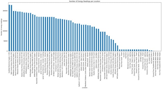
Figure 1. Number of electricity consumption records in the dataset, per council building.

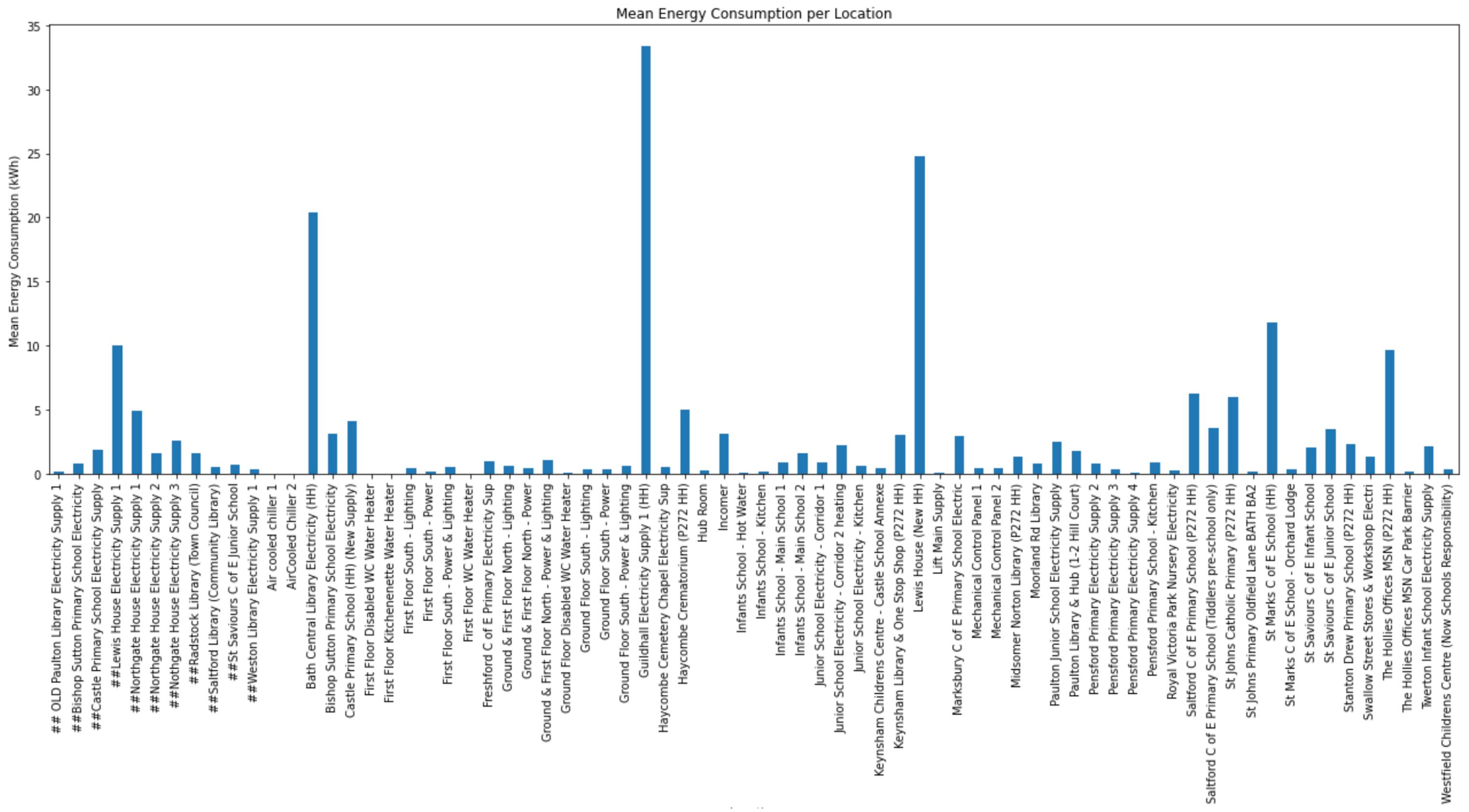
Figure 2 presents the mean energy consumption of each building with a 30 min interval. The dataset proved to be highly unbalanced, with some buildings being higher than 20 kWh while others are close to 0 kWh. This introduces real-world scenarios to the project, as the model to be trained must be implemented in communities with diverse consumption patterns among their members.

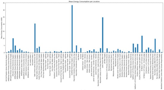
Figure 2. Average energy consumption for each building in half-hour intervals.

As the Solcast API offers weather data from various global locations and our available energy readings are specific to Bath, UK, we submitted a request solely for a dataset corresponding to the coordinates 51.378102, −2.359683, representing the city of Bath. The dataset covered the period from 1 January 2007 to 8 February 2020, with a granularity of 30 min, aligning with the BANES dataset.

The dataset included essential variables such as Air Temperature, Relative Humidity, and DNI (solar irradiation). It is worth noting that although DNI is not utilized in the consumption forecast model, it was included because estimating the REC potential solar panels energy production relies on it.

Subsequently, we merged the BANES dataset with the Solcast dataset. To ensure consistency, the relative humidity column was divided by one hundred, transforming the scale from 0 to 100 to a range of 0 to 1. The final aggregated dataset includes the following features: time, location, RelativeHumidity, AirTemp, energy and DNI.

3.2. Methodology

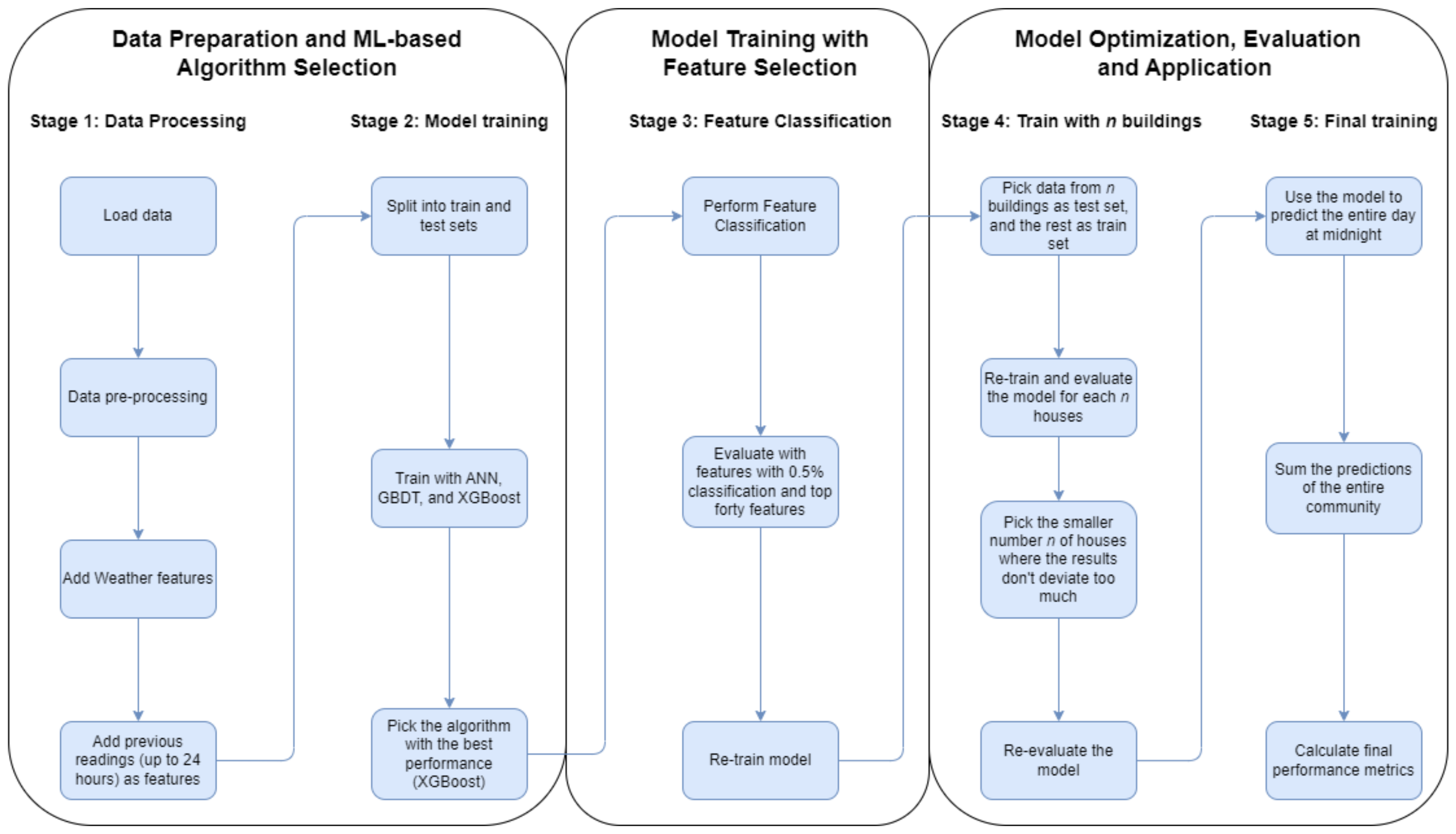
The methodology of the energy consumption forecast, which is illustrated in Figure 3, consists of five phases: Data Processing, Model Training, Feature Classification, Training with n buildings, and Final Training. In the first stage, the data are retrieved and processed as explained in Section 3.1. Then, for each consumption reading, the previous readings (up to 24 h) were added, in order to be considered as features. The second stage consisted of splitting the data into train and test subsets, where the train data were used to train different models, using ANN, GBDT, and XGBoost algorithms, and the test data were used to evaluate the algorithms and identify the one with the best performance. In this case, XGBoost performed better than the other algorithms, and was therefore picked to be used in the next phases. Next, a Feature Classification technique was applied to give a score to each feature according to its importance. Then, the selected model was re-evaluated with the top forty features and with features with at least 0.5% importance classification, with the latter being picked for the next stages. The fourth stage consists of an alternative approach to model training where, instead of randomly splitting the whole time window between train and test sets, n random buildings were picked as the test data, and the remaining as train data. An experiment was carried out, in order to know the minimum number n of random buildings that is necessary for the results to have a small variation. The final model is then trained and re-evaluated. The final stage consists of using the model to predict the entire day at midnight for each individual building, instead of constantly predicting the short-term forecast, and then summing up the predictions for the entire community and calculating the final performance metrics. All these steps will be better described in the following sections.

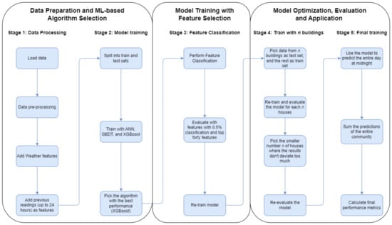
Figure 3. Proposed methodology for electricity consumption forecast.

4. System Architecture

This section presents the system architecture for the energy management system of the REC, as well as the trained ML-based model for electricity consumption forecast and the decision-making algorithms utilized in the REC’s energy management system.

4.1. REC Energy Management System

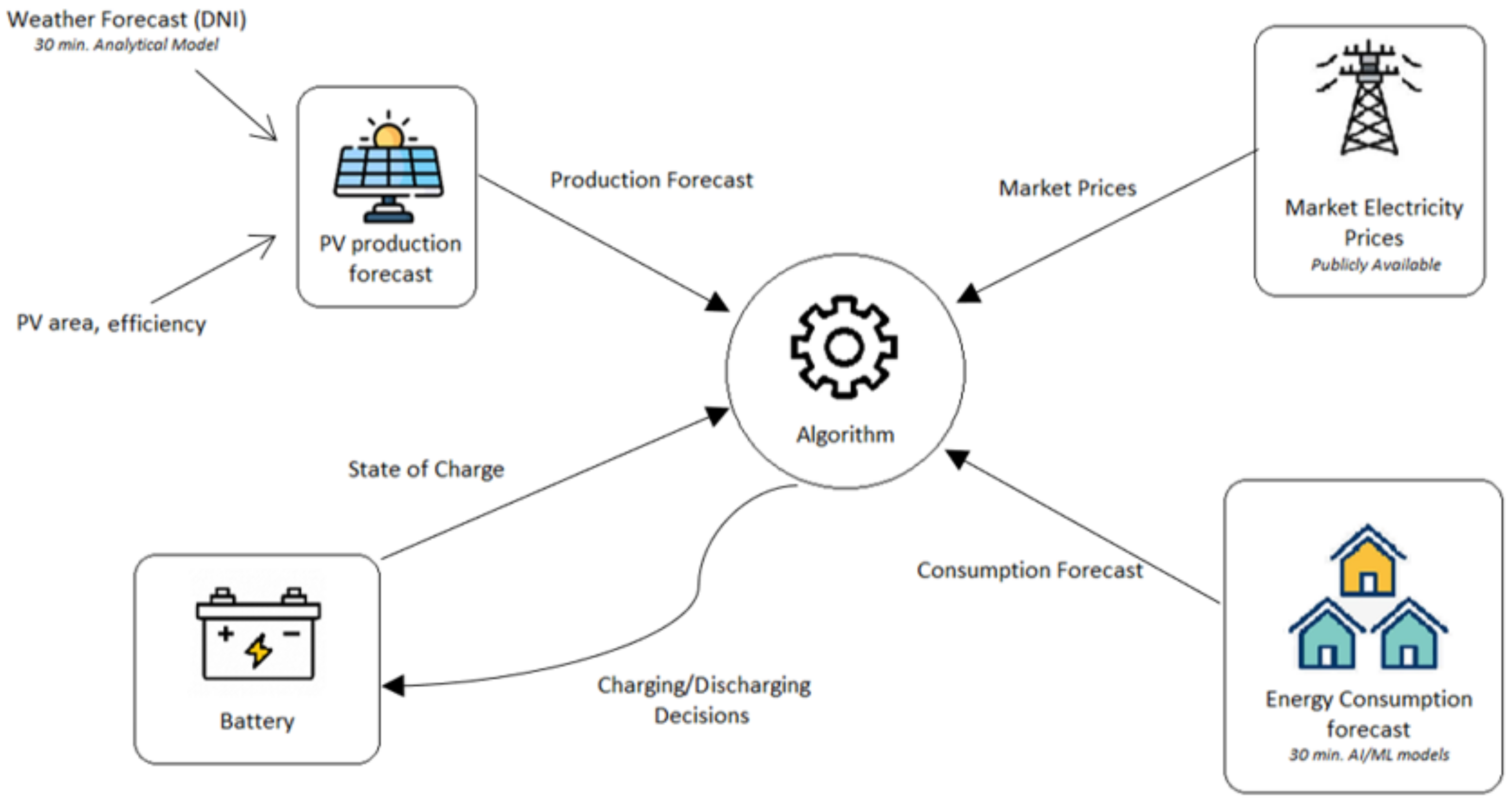
Considering the objectives outlined and the related studies, an architecture for the REC management system is put forward in Figure 4. At the center, a decision-making algorithm is responsible for taking charging and discharging of REC storage device (e.g., second-life batteries) decisions. Therefore, it manages what the community should do, regarding the energy produced, stored, and the energy that must be fetched from or given to the grid. The decision algorithm is executed twice per hour, and receives the output of the remaining components as input.

Figure 4. REC management system architecture.

The algorithm is fed with a forecast of the PV panels’ production, as well as the energy consumption predicted by the AI/ML model. The forecast of PV panels is provided by an analytical model that estimates the energy production of a REC based on the prediction of the solar irradiance and the area and efficiency of the PV panels. The utilization of AI/ML models for energy consumption forecasting aims to enhance the utilization of green energy and decrease the overall electricity cost. This is achieved by estimating whether the available energy production and battery charge are sufficient to meet the predicted consumption by the Renewable Energy Community (REC) in the upcoming 24 h.

The algorithm takes into account market electricity prices, using this information to guide decisions on when to purchase, sell, or store energy. The inclusion of current and day-ahead electricity prices influences the timing of specific energy management operations throughout the day.

It is noteworthy that a member of the Renewable Energy Community (REC) is a prosumer capable of generating and/or storing energy in a storage device, such as a battery. Therefore, the algorithm utilizes information from battery modules, specifically the state-of-charge, which indicates the current charge level of the batteries. The algorithm interfaces with this component to determine whether the batteries should be charged or discharged at any given moment. This pivotal decision is made by the algorithm to optimize the REC’s target objectives, such as attaining a specific percentage of local renewable energy and minimizing the overall electricity bill.

4.2. ML-Based Electricity Consumption Forecast

There is no consensus in the literature regarding the ML-based model that is considered the best to predict electricity consumption. Therefore, in this work, several techniques were considered, namely Gradient Boost, XGBoost and ANN, which were often presented in the related works, providing satisfactory results. In order to select the most appropriate model for the consumption forecast, Gradient Boost, XGBoost and ANN were trained and tested under similar circumstances by providing short-term electricity consumption at every location.

The algorithms utilized a dataset comprised 50 columns, including air temperature, relative humidity, and 48 columns of previous energy consumption in steps of 30 min, e.g., 30 min, 60 min, 90 min, and so on, up to the previous 24 h. The dataset was divided into train and test sets with 80% for training and 20% for testing. The ML algorithms were parameterized as follows:

• The ANN model included four layers, with the input layer having 50 neurons, one for each feature. There were also two hidden layers, each one with a size of ten neurons and using a ReLU activation function. The training of the model employed the Adam optimizer with Mean Squared Error (MSE) serving as the loss metric. The training process involved 20 epochs and utilized a batch size of 1000.
• In the case of Gradient Boost, training involved 100 estimators and a learning rate of 0.1, as outlined in [23].
• XGBoost was trained with a maximum depth of 6, learning rate of 0.3, and 100 estimators. The other hyperparameters used the default values. The training was performed using GPU. Running the algorithm on GPU increased the performance of the training time.

More information on the performance of these three ML models applied to the dataset used in this work will be presented in Section 5.

4.3. PV Production Forecast

In order to estimate the solar production of the REC’s PV panels in the next hours, an analytical model based on the solar irradiance forecast was employed. This model is based on the work of Filik et al. [24] and the Direct Normal Irradiance (DNI) values were obtained from Solcast API, as mentioned in Section 3. Three different production scenarios were considered for the whole REC: high, low (equivalent to one-tenth of the high production), and average (the mean between high and low production). The high production scenario featured a total area of 28.8 m² (comprising eighteen panels, each measuring 1.6 m²) per REC member, and a yield of the solar panel of $0.16$. Under standard conditions, characterized by a performance coefficient of 1 and solar irradiance of 1 kWh/m², the estimated energy output would be approximately 4.6080 kWh. Consequently, in the low production scenario, it would generate approximately 0.4608 kWh of energy, while an average scenario would yield around 2.5344 kWh. Additionally, PV performance was considered the same for the three scenarios, with a value of 0.95. Also, for simplicity, it was assumed that there were no errors associated with weather forecasts or the model’s predictions.

Besides electricity generation, the prosumers in a REC may also have the ability to store energy. The total storage capacity of the community depends not only on the number of batteries, but also on their individual capacities. Drawing from real-world examples of solar batteries, three storage scenarios were defined: small (1.6 kWh), medium (6.4 kWh), and large (12.8 kWh) storage capacity for each of the REC members.

4.4. Decision-Making Algorithm

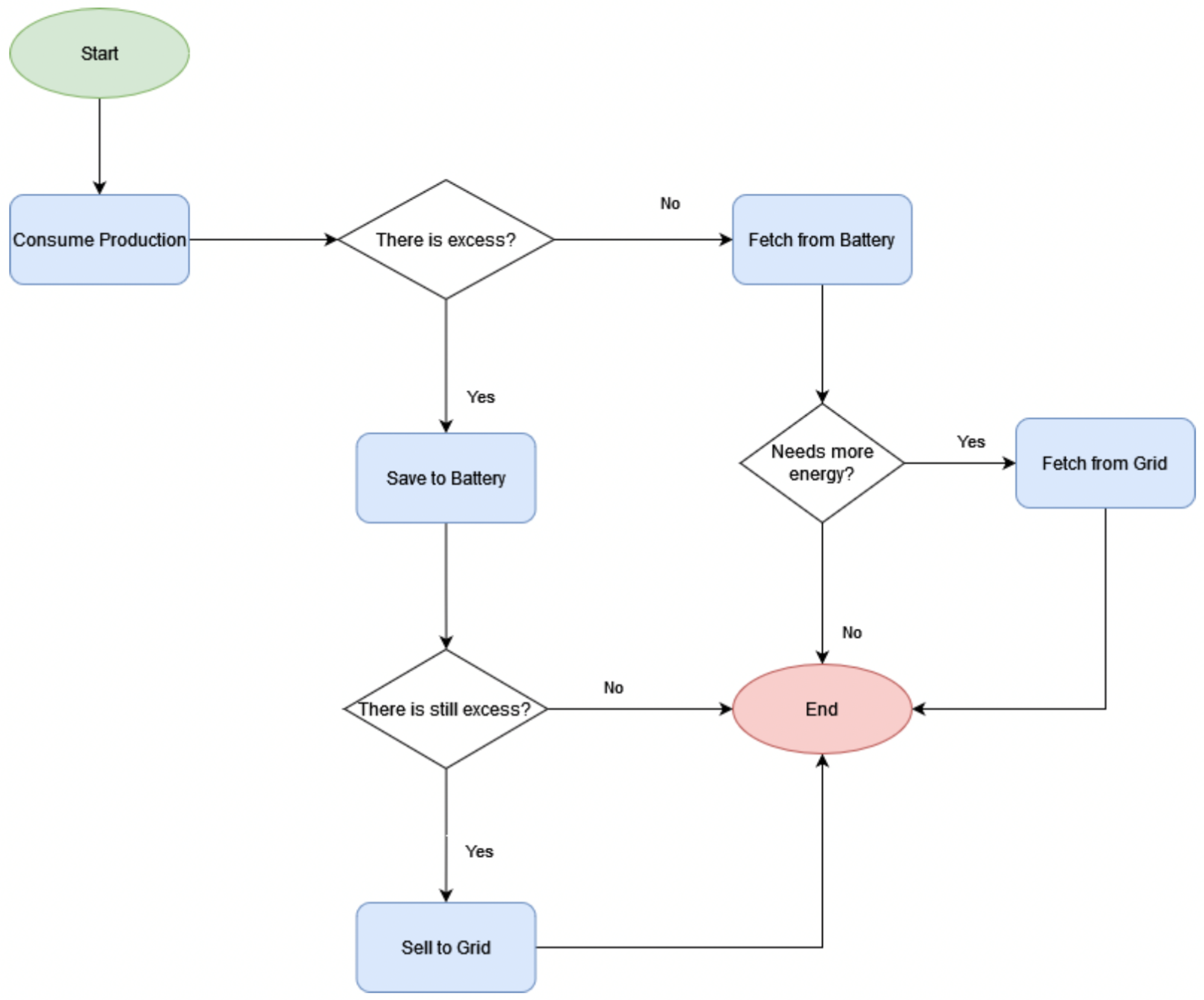
The decision-making algorithm at the center of Figure 4 was developed from a baseline scenario to a more complex and efficient management of the energy resources available at the REC. Thus, three distinct algorithms were considered in this evolution towards reducing the electricity costs of the REC. All of them make decisions of whether to buy, sell or store energy every 30 min. The initial algorithm serves as the baseline approach, operating on a half-hourly basis to manage energy consumption without incorporating any storage capability or machine learning. When additional energy is required, it is procured from the grid as necessary. The second algorithm represents an enhanced iteration of the baseline algorithm, introducing the option to store surplus energy in batteries. As depicted in Figure 5, this system utilizes the energy it generates, but in cases of excess production, it channels that surplus into the battery until its capacity is reached. Any surplus energy beyond this point is then sold to the grid at a fixed rate of EUR 0.03 per kilowatt-hour (EUR/kWh). In instances where there is no excess energy production and additional power is still required, the system will discharge the battery and draw from it, while also obtaining the remaining needed energy from the grid.

Figure 5. Battery consumption algorithm flowchart.

Figure 6 presents the final and more complex algorithm, which is based on the machine-learning model for the electricity consumption forecast. This forecast is then used to determine the optimal moments for charging and discharging the batteries. This algorithm is inspired in the work of Pholboon et al. [25], and follows a strategy of acquiring energy from the grid during periods of lower electricity prices, typically on a bi-hourly tariff basis. At midnight each day, it initiates a forecasting model for both energy production and consumption, projecting these values for the upcoming day. Based on these forecasts, the algorithm executes one of three potential actions. In scenarios where the estimated production surpasses the predicted consumption between 9:00 and 18:00, and the surplus falls within the limits of the battery capacity, it proceeds to fetch energy from the grid to charge the battery. The amount acquired from the grid corresponds to the battery’s capacity minus the estimated surplus.

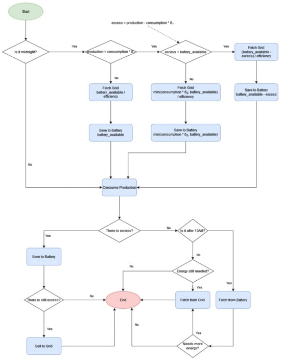
Figure 6. ML-based algorithm flowchart.

In situations where the algorithm foresees an excess of solar energy beyond the battery’s storage capacity, it will retrieve electricity from the grid to align with the projected morning consumption while reserving any surplus energy for later storage in the battery. Conversely, when there is no expected of surplus solar energy throughout the day, the battery will be charged to its full capacity in advance.

Afterwards, and up until 10:00 a.m., each iteration of the algorithm prioritizes the utilization of the energy that has been generated. If there is surplus, it will be directed into the battery until reaching its full capacity. Any surplus beyond this point will be sold to the grid at a price of EUR 0.03 per kilowatt-hour (EUR/kWh). However, if there is no surplus production, the algorithm will instruct the system to fetch energy from the grid. Once it is 10:00, the algorithm will also command the system to consume the produced energy. Nevertheless, if there is a demand for energy, the system initially draws the required energy from the battery before resorting to grid consumption. In the case of excess production, the system follows the earlier procedure before 10:00, storing the surplus energy in the battery and, if applicable, selling the remaining excess to the grid.

In the flowchart of Figure 6 and according to the work of Pholboon et al. [25], ${\delta }_1$ represents the ratio between the predicted energy consumption between 9:00 to 18:00 and the estimated consumption for the whole day, while ${\delta }_2$ is the energy forecast of the morning between 6:00 and 9:00 divided by the consumption forecast of the day. These heuristics enable an optimized and efficient management of the energy in the community, by helping estimate the amount of electricity that is required to buy from the grid and store in the batteries when the price of energy is cheaper, i.e., during the night.

Therefore, the main goal of this decision-making algorithm is to reduce the overall electricity bill of the community on a daily basis, by attempting to optimize the following cost function:

$$\begin{array}{cc}\hfill cost=& consumptio{n}_{midnight}\ast buy\_pric{e}_{midnight}+battery\_losse{s}_{midnight}\hfill \\ & +\sum _{i=1}^{48}(consumptio{n}_i\ast buy\_pric{e}_i-surplu{s}_i\ast sell\_pric{e}_i+battery\_losse{s}_i)\hfill \end{array}$$

(1)

The electricity cost calculation in Equation (1) is obtained by adding the cost of buying the electricity in advance, to store it in the batteries at midnight, with the sum of the 48 electricity exchanges that take place during the day corresponding to all 30 min intervals. The consumption variable represents the energy consumed from the public grid, while the surplus is the electricity sold to the grid. The battery_losses represent the inverter losses, when the system charges or discharges the batteries (an efficiency of 97% was considered). The buy_price value may vary during the day depending on the tariff, while the sell_price was considered to be a fixed value (0.03 EUR/kWh), as previously mentioned.

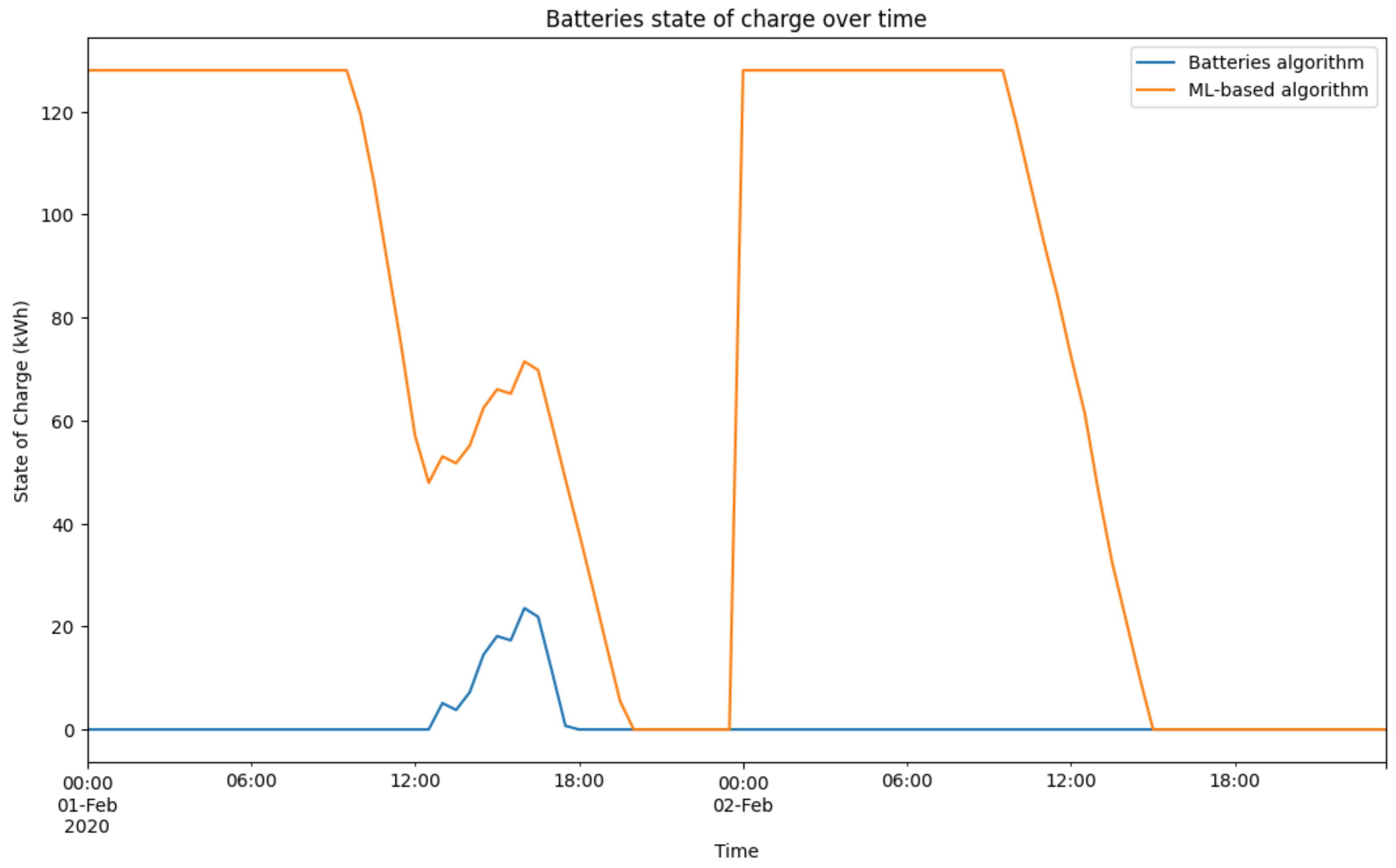
For better understanding of this algorithm’s operation, Figure 7 illustrates the evolution of the batteries state of charge over a time interval of 48 h, for a specific example during the first two days of February 2020. It compares the behavior of the simple batteries algorithm with the ML-based one for a scenario with high storage capacity (128 kWh) and high PV generation (4.6080 kWh). In the ML-based algorithm, it is possible to observe that, in this example, the batteries are totally charged at midnight, and only start to be discharged after 10:00 until being fully depleted. In the first day, there is surplus PV production that is stored in the batteries between 12:00 and 18:00. On the other hand, there is no solar generation surplus in the second day and, therefore, the batteries are not charged during the daytime.

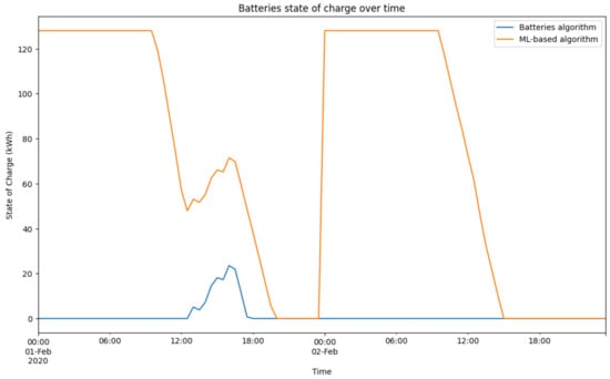
Figure 7. Batteries’ state of charge evolution over 48 h interval.

5. Assessment Results

After implementing the above architecture and associated decision-making algorithms, the devised system was evaluated starting with a performance comparison between different machine-learning models applied to the forecast of electricity consumption in the energy community. Then, an assessment of the proposed algorithms for energy management in the REC was carried out with a strong focus on the cost reduction of the electricity bill under different scenarios (low to high PV production and low to high battery capacity).

5.1. Electricity Consumption Forecast

After completing the training and testing phases, the algorithms’ performance was evaluated by comparing six different metrics: the time taken for the training phase, the time taken for predicting the test dataset, Mean Squared Error (MSE), Root Mean Squared Error (RMSE), Mean Absolute Error (MAE), Weighted Absolute Percentage Error (WAPE), and $R^2$. Table 2 presents the results of these metrics. They confirm that all the algorithms perform well, particularly XGBoost, which performs better than the others in all metrics, and was therefore chosen as the model for the electricity consumption forecast. In terms of computational complexity, it can be observed that XGBoost presents significantly lower training and prediction times when compared to the other algorithms. This is particularly relevant for the measured training time, which was less than 1 min for the XGBoost model, while it took more than 3 h for the GBDT algorithm. This can be explained since XGBoost trains the models of its ensemble in parallel. In scenarios where the forecast models need to be constantly retrained or newly generated, this might become an important factor, although this metric could be further improved if more powerful hardware is employed, since in this case a regular desktop was utilized for the measurements.

Table 2. Outcomes of predictions on the test dataset.

	ANN	GBDT	XGBoost
training time (s)	268.7992	11,676.7068	54.2282
prediction time (s)	45.1752	8.1269	1.9277
MSE (kWh)	0.8107	0.9097	0.6629
RMSE (kWh)	0.9004	0.9538	0.8142
MAE (kWh)	0.3601	0.3683	0.3290
WAPE	8.9294	9.1313	8.1575
$R^2$	0.9886	0.9872	0.9907

The best result for each metric is presented in bold.

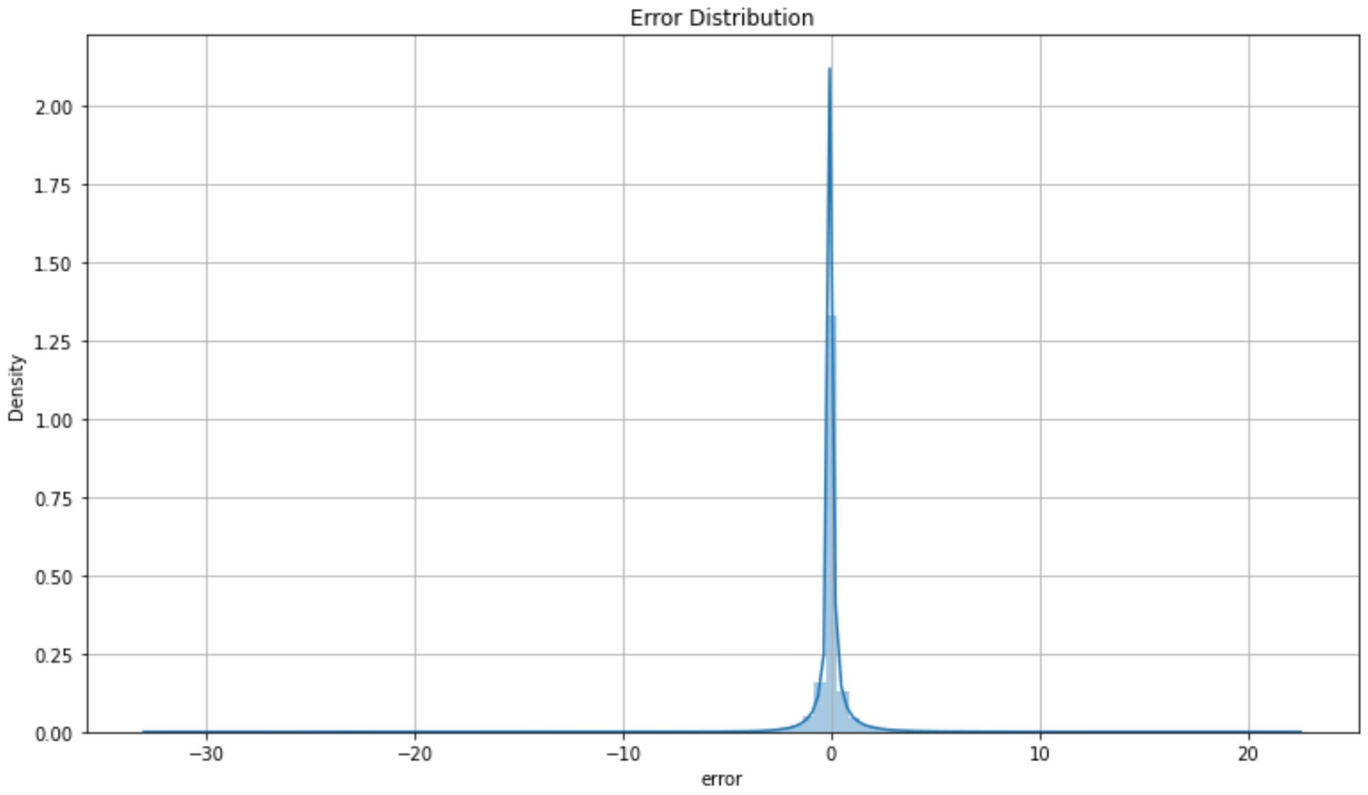
In addition, Figure 8 demonstrates that the majority of the error is centered around zero. As a result, the focus of the remaining work was to optimize the XGBoost model. Applying a method known as Feature Classification, a reduced set of features was chosen based on their significance in training an XGBoost model, following the steps outlined in [19]. To this end, instead of using the previous 24 h consumption values like in the algorithms’ comparison test, the entire previous week was used, resulting in 336 consumption-related features, plus the air temperature and relative humidity, totaling 338 input parameters. The features have a name $energy\_la{g}_i$, where i represents the ith previous half-hour reading.

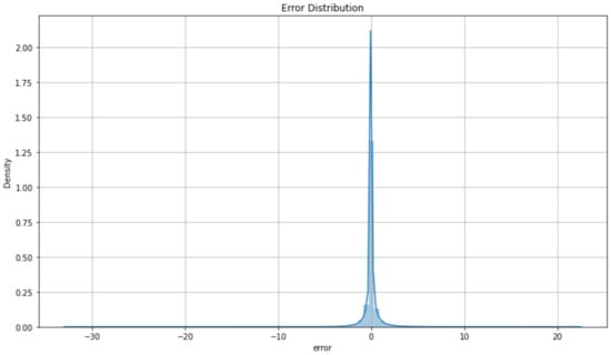
Figure 8. Distribution of errors in the XGBoost model trained using the preceding 24 h and weather metrics.

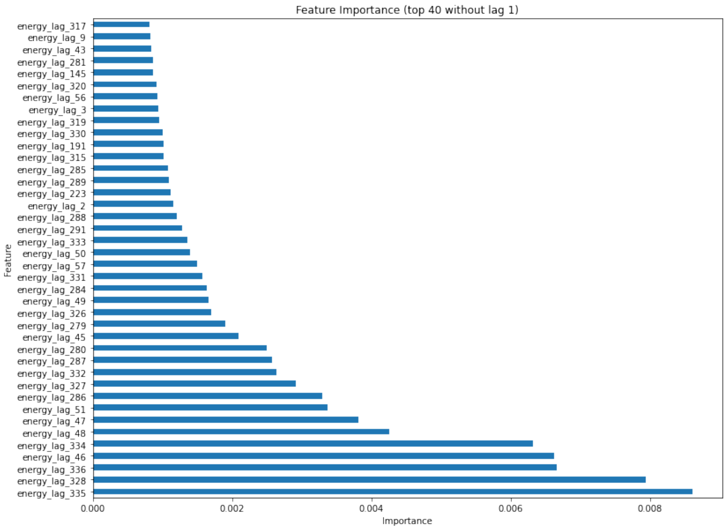
Examining the importance classification of the top forty features reveals that the most significant influence on the algorithm comes from the direct preceding energy measurement, with a score exceeding 80%, surpassing every other feature by a considerable margin. Figure 9 presents the graph with the most important features without the $energy\_la{g}_1$ feature. As can be seen, the most crucial features are those corresponding to the same hours in the week before and the day before. With the results of the features’ classification, two models were trained: one with the forty most prominent features, and another with the six most important features, which have an importance classification of over 0.5%. The training phase was conducted in a manner similar to previous iterations, involving the division of the data into training and test datasets with an 80% and 20% ratio, respectively. The hyperparameters of the XGBoost algorithm were enhanced for both models, through the analysis of some different values combinations, although not employing extensive hyperparameter optimization. As a result, the following hyperparameters values were selected: 1000 estimators, with a maximum depth of 5, and a 0.05 learning rate. Table 3 presents the performance metrics results.

Figure 9. The 40 features, excluding energy lag 1, with the most significant importance classification.

Table 3. Performance metrics on the testing dataset using XGBoost model (>0.5% vs. top 40 features).

	Feature Importance > 0.5%	Top Forty Features
training time (s)	11.4464	42.7416
prediction time (s)	0.7795	1.2840
MSE (kWh)	0.7200	0.5372
RMSE (kWh)	0.8485	0.7329
MAE (kWh)	0.3320	0.3006
WAPE (%)	8.1936	7.4197
$R^2$	0.9899	0.9925

The best result for each metric is presented in bold.

Besides that, a different approach was also followed in which n different buildings were left out of the training phase and used to evaluate the model. This approach was followed since, in a real-life scenario, the model to be used on the consumption forecast of a REC may not be trained with the specific data of that REC, but with the data from other communities, at the least during the beginning of the REC operation. This cross-validation technique also helps to prevent overfitting, by randomly selecting n buildings for testing, leaving the remaining ones for training, thus effectively splitting the dataset into training and testing data. To determine the minimum acceptable number of buildings for testing, various models were trained by excluding 5, 10, and 15 randomly chosen buildings. This training utilized only the features with an importance classification higher than 0.5%. Table 4 shows the results of these experiments, in which each value represents the average of five tests with a distinct and independent set of buildings. It presents the mean ($\overline{x}$) and standard deviation ($\sigma$) of each assessed metric. As can be seen, the standard deviation of the error metrics when only 5 buildings are used is significantly larger than those with 10 or 15 buildings. Therefore, it can be concluded that the model can not be evaluated with such small number of buildings. On the other hand, when 10 or 15 buildings are employed, the performance metrics of all five tests recorded similar values. Therefore, for this approach, at least a minimum of ten buildings must be used as data for testing.

Table 4. Performance metrics with 5, 10 and 15 buildings as test data.

	$\overline{\mathit{x}}$	$\mathit{\sigma }$	$\overline{\mathit{x}}$	$\mathit{\sigma }$	$\overline{\mathit{x}}$	$\mathit{\sigma }$
training time (s)	13.2876	0.5850	11.7588	0.6424	10.8585	0.5653
prediction time (s)	0.5733	0.2018	0.9884	0.1307	1.0647	0.1695
MSE (kWh)	0.9366	1.2303	0.7529	0.0923	0.7087	0.0234
RMSE (kWh)	0.8458	0.5260	0.8664	0.0524	0.8417	0.0138
MAE (kWh)	0.3724	0.2597	0.3354	0.0090	0.3317	0.0019
WAPE (%)	12.7974	5.2622	8.2773	0.2220	8.1865	0.0457
$R^2$	0.9528	0.0336	0.9895	0.0013	0.9901	0.0003

The best results for each metric are presented in bold.

Finally, this approach was repeated with the forty features presenting highest importance, by using ten buildings to assess the model performance. Table 5 compares the metrics of the models trained with the features presenting an importance higher than 0.5% against the case of using the top forty most important features, when ten buildings are left out for the testing data. As can be observed, the difference in terms of forecast accuracy is not very significant, indicating that the model can be trained using the six features with more than 0.5% feature importance, without relevant performance degradation.

Table 5. Consumption forecast performance for ten buildings (>0.5% vs. top 40 features).

	Feature Importance > 0.5%	Top Forty Features
training time (s)	11.0428	40.1057
prediction time (s)	1.2434	1.6760
MSE (kWh)	0.2370	0.1635
RMSE (kWh)	0.4868	0.4044
MAE (kWh)	0.2098	0.1865
WAPE (%)	9.9973	8.8847
$R^2$	0.9798	0.9860

The best result for each metric is presented in bold.

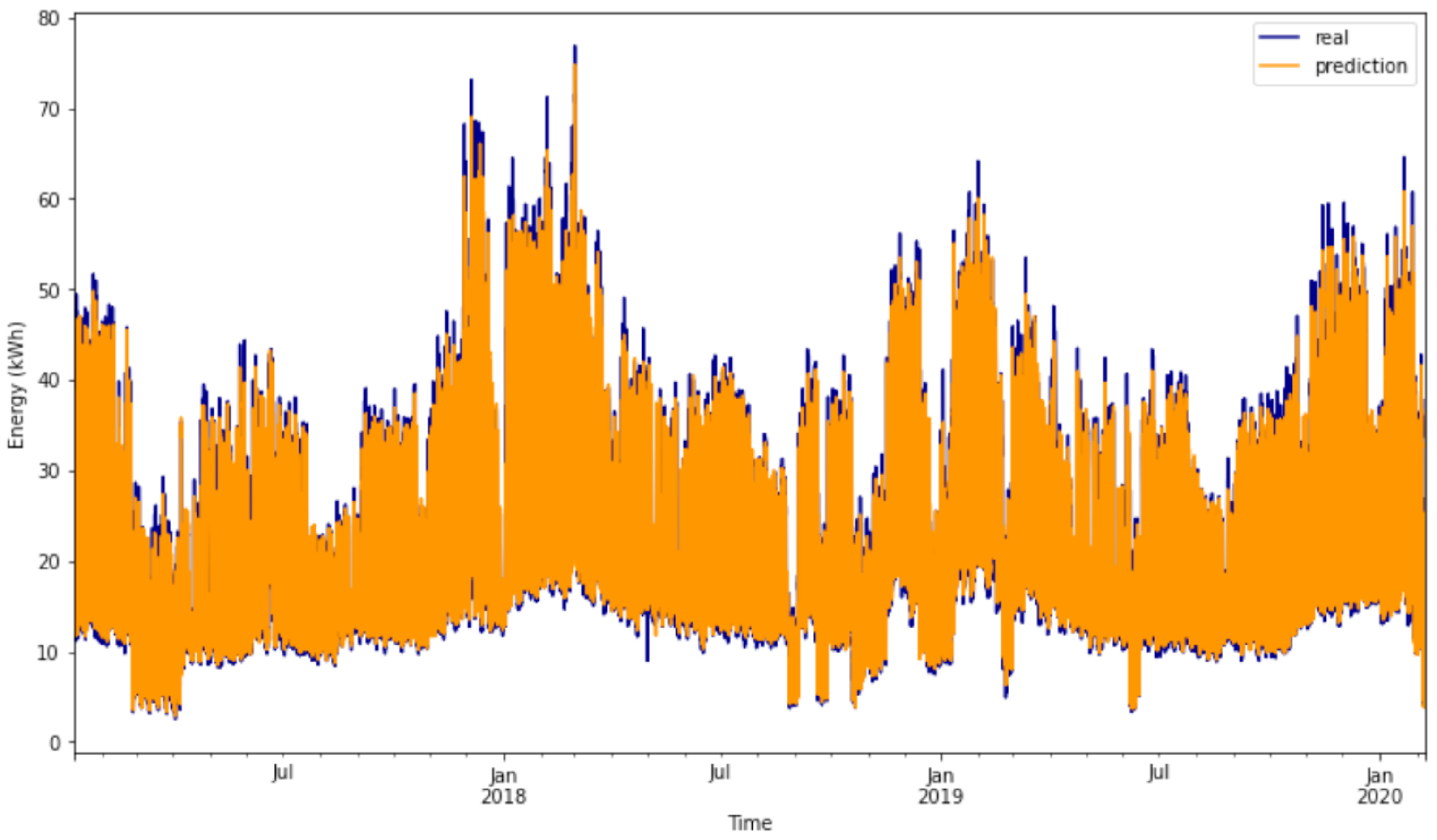
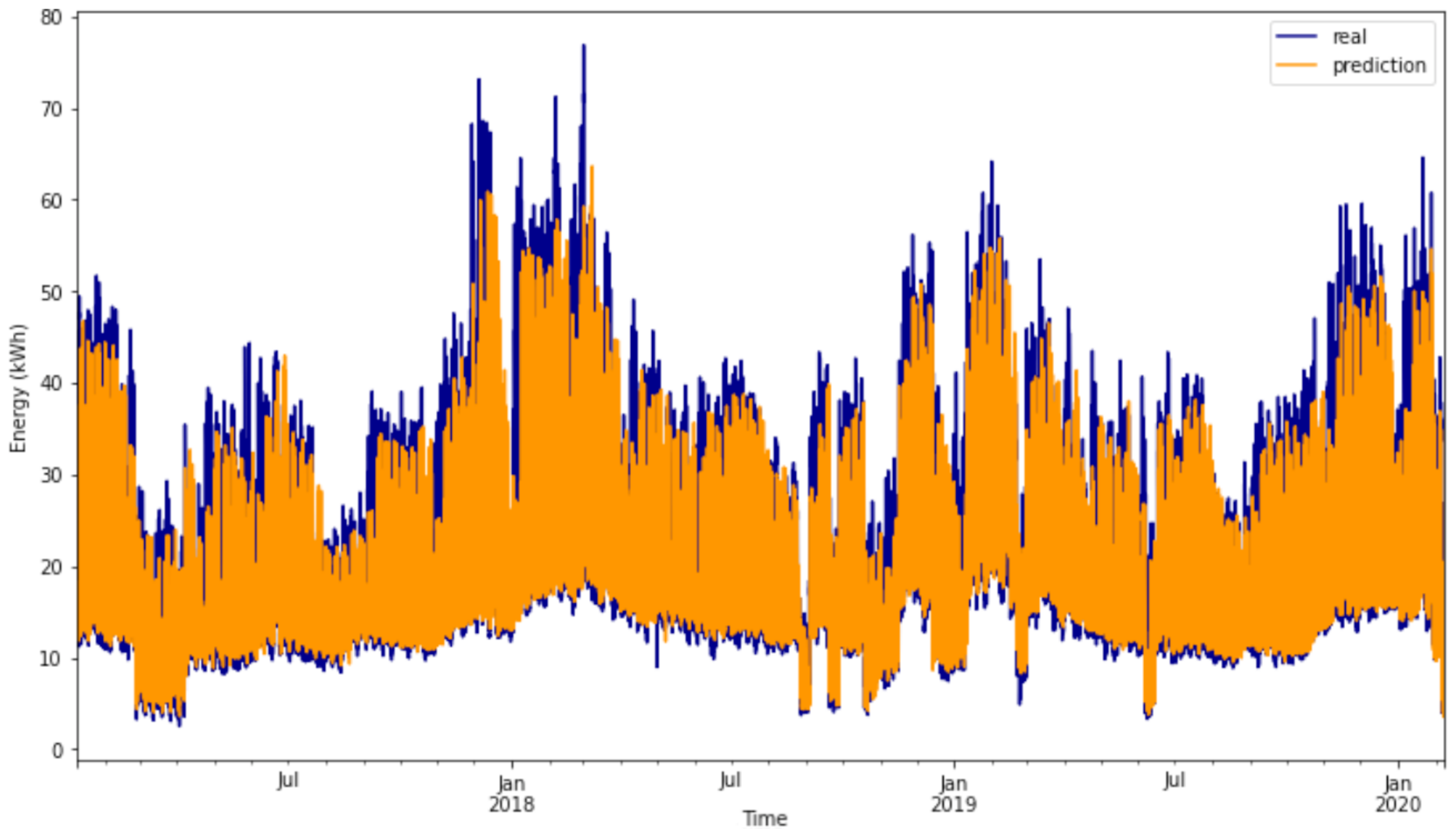
While these results pertain to the short-term consumption of individual buildings, the primary objective of this project is the management of the entire community. Consequently, the individual building forecasts hold less significance compared to the aggregate consumption of the community. Following the algorithm’s prediction of individual building consumption, the actual forecast for REC electricity consumption is derived by summing these individual predictions. Additionally, the algorithm must anticipate the consumption for the entire next day at midnight. This entails forecasting short-term consumption at midnight using real values, and subsequently predicting the next steps with real values whenever available or relying on the previously predicted values, thereby propagating any errors. Table 6 outlines the performance metrics for two scenarios: one where the algorithm predicts the short-term forecast of the community and another where it predicts the entire day at midnight. In both cases, the values for each building are grouped and summed. The comparison between short-term and full-day forecasts against the actual values is depicted in Figure 10 and Figure 11, respectively. While full-day forecasting falls short compared to short-term forecasting, it still maintains a similar pattern with the real values.

Table 6. Forecast performance metrics for community (aggregate of 10 buildings as testing data) electricity consumption (short-term vs. full-day).

	Short-Term Forecast	Full-Day Forecast
MAE (kWh)	1.1819	2.6361
MSE (kWh)	3.1929	17.0603
RMSE (kWh)	1.7869	4.1304
WAPE (%)	6.1067	13.3331
$R^2$	0.9700	0.8396

Figure 10. Short-term forecasts compared to real values for the aggregate of 10 buildings as testing data.

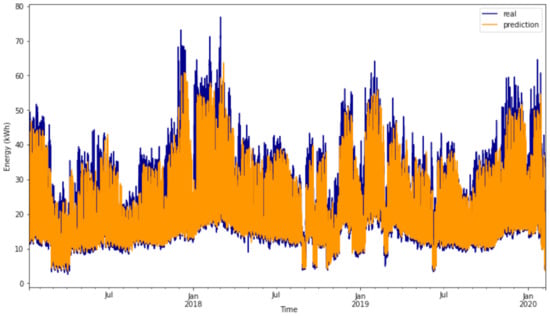
Figure 11. Full-day forecasts compared to real values for the aggregate of 10 buildings as testing data.

5.2. PV Production Forecast

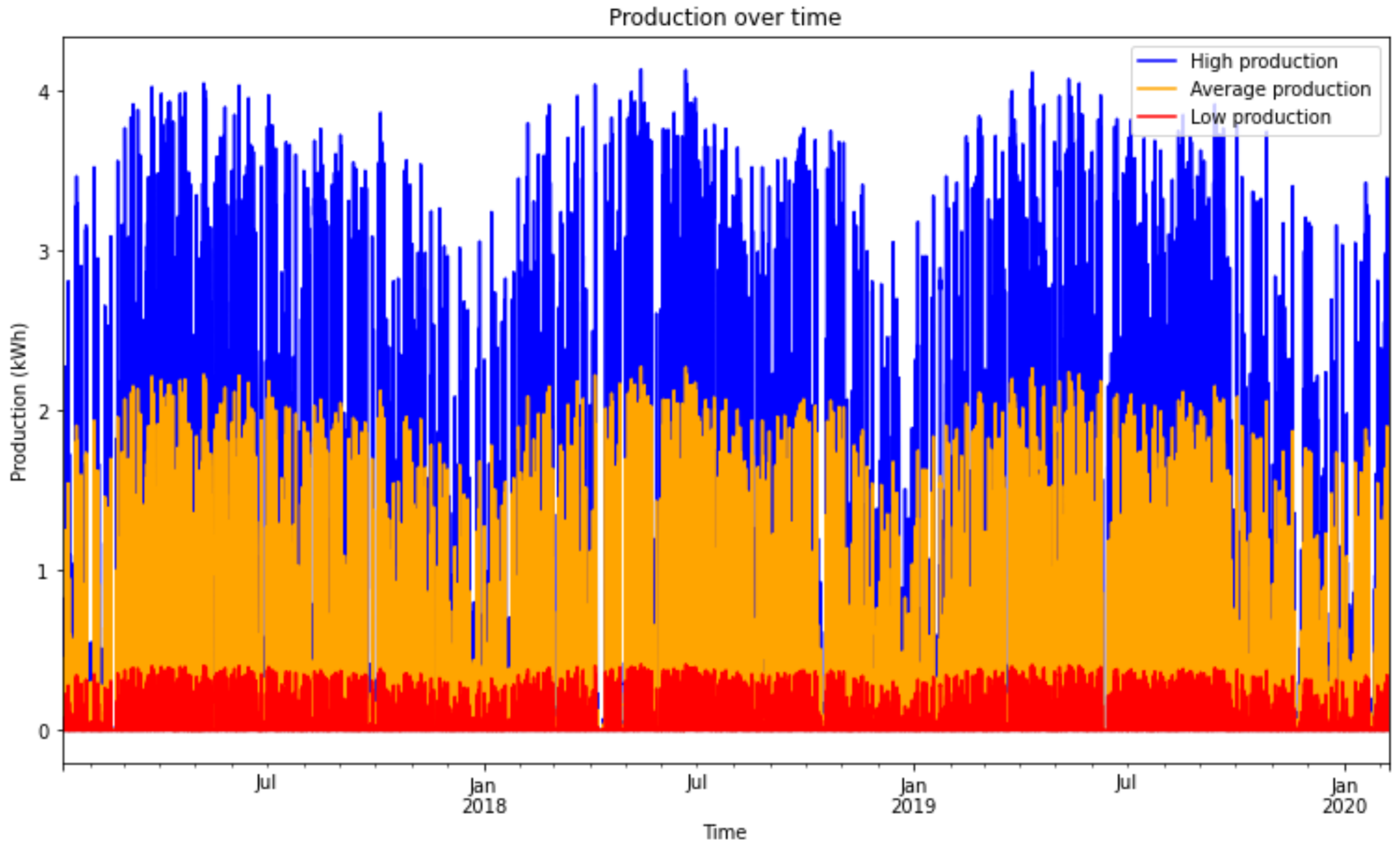
The electricity production forecast derived from the analytical model are presented in Figure 12. These are based on the DNI obtained from the Solcast API and applied to three different scenarios: high, average and low production for each building of the REC. Additionally, Table 7 furnishes details regarding the model results, encompassing the mean ($\overline{X}$), standard deviation ($\sigma$), and sum ($\Sigma$), along with the minimum and maximum values and percentiles. Ultimately, the output is scaled by the number of buildings within the community.

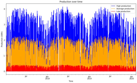
Figure 12. PV panels’ electricity generation per building over time.

Table 7. Analytical model results for PV panels’ output (high, low and average production scenarios).

	High Production (kWh)	Low Production (kWh)	Average Production (kWh)
$\overline{x}$	0.4320	0.0432	0.2376
$\sigma$	0.9680	0.0968	0.5324
Min	0.0000	0.0000	0.0000
25%	0.0000	0.0000	0.0000
50%	0.0000	0.0000	0.0000
75%	0.0744	0.0074	0.0409
Max	4.1368	0.4136	2.2752
$\Sigma$	23,352.8281	2335.2828	12,844.0555

5.3. Market Prices

Regarding the electricity market prices, three distinct tariffs were considered, following the most common rates existing in the market: simple, bi-hourly (weekly cycle) and bi-hourly (daily cycle). For all the tariffs, the following prices were assumed constant for the whole dataset: $0, 1583$ EUR/kWh in the simple tariff scenario, $0, 1917$ EUR/kWh in the peak hours of bi-hourly tariffs and $0, 1044$ EUR/kWh out of the peak periods. By applying these tariffs, the average price paid by each building over time since the beginning of the dataset is presented in Table 8. It shows the sum ($\Sigma$), mean ($\overline{x}$), and standard deviation ($\sigma$), as well as the minimum and the maximum values, and the percentiles of the average values paid by a REC member.

Table 8. Average electricity price results for bihourly (daily), bihourly (weekly) and simple tariffs.

	Bihourly Tariff (Daily) (EUR)	Bihourly Tariff (Weekly) (EUR)	Simple Tariff (EUR)
$\overline{X}$	1.2443	1.2344	1.2003
$\delta$	0.9680	0.0968	0.5324
Min	1.8411	1.8388	1.5997
25%	0.3369	0.3044	0.3941
50%	0.5800	0.6037	0.6106
75%	1.3634	1.2706	1.0751
Max	4.1368	0.4136	2.2752
$\Sigma$	285,857.4185	283,567.7304	275,740.5707

5.4. Decision-Making Algorithm

The decision-making algorithms were evaluated and compared in terms of total REC electricity bill and energy self-sufficiency. These algorithms underwent testing with a community comprising ten buildings, which were excluded from the training phase for the electricity consumption forecast component. Evaluation was carried out across three scenarios of storage capacity and three scenarios of PV generation.

The baseline algorithm underwent assessment using ten buildings in the dataset, covering the period from 8 January 2017 to 7 February 2020. As indicated by the results in Table 9, the PV generation facilitates savings exceeding 160,000 kWh in REC grid consumption over the three-year period when production is high, compared to the low production scenario. This translates to a difference of more than EUR 25,000 when employing the simple tariff (the lowest in all scenarios).

Table 9. Total bill cost and grid consumption for high, low, and average production scenarios, using the baseline algorithm.

PV Generation		Baseline
High Production	Bihourly tariff (weekly option) (EUR)	146,364.0864
	Bihourly tariff (daily option) (EUR)	146,434.8987
	Simple tariff (EUR)	144,322.7950
	Consumed From Grid (kWh)	911,704.3270
Low Production	Bihourly tariff (weekly option) (EUR)	176,246.0450
	Bihourly tariff (daily option) (EUR)	175,254.3673
	Simple tariff (EUR)	169,883.2251
	Consumed From Grid (kWh)	1,073,172.6156
Average Production	Bihourly tariff (weekly option) (EUR)	158,095.2314
	Bihourly tariff (daily option) (EUR)	158,055.0320
	Simple tariff (EUR)	154,340.5272
	Consumed From Grid (kWh)	974,987.5379

Table 10 shows the results for the low, average and high storage capacity scenarios, when the batteries algorithm is executed, considering also the scenarios for high, low, and average PV generation. As before, the total bill cost of the three possible tariffs and the grid consumption are presented.

Table 10. Total bill cost and grid consumption for 16, 64 and 128 kWh storage scenarios, using the batteries algorithm.

Production	Tariff	16 kWh	64 kWh	128 kWh
High	Bi-hourly (weekly) (EUR)	140,829.1992	138,906.5757	137,912.5288
	Bi-hourly (daily) (EUR)	141,125.5911	139,523.4337	138,594.9123
	Simple (EUR)	139,058.6055	137,474.3989	136,286.6575
	Grid consumption (kWh)	903,360.8796	890,829.1492	881,433.6229
Low	Bi-hourly (weekly) (EUR)	176,245.0032	176,245.0083	176,245.0083
	Bi-hourly (daily) (EUR)	175,253.4215	175,253.4243	175,253.4243
	Simple (EUR)	169,882.2200	169,882.2242	169,882.2242
	Grid consumption (kWh)	1,073,171.5146	1,073,171.5413	1,073,171.5413
Average	Bi-hourly (weekly) (EUR)	156,903.2119	156,547.5470	156,454.1503
	Bi-hourly (daily) (EUR)	156,989.9957	156,757.9280	156,685.2525
	Simple (EUR)	153,228.0538	152,930.9751	152,805.2904
	Grid consumption (kWh)	972,550.0141	970,189.6801	969,195.4626

The best result for each combination of production scenario and electricity tariff is presented in bold. The best result for each production scenario and for all electricity tariffs is presented in italic.

The same approach was followed for the ML-based algorithm. This algorithm, however, does not have the goal of reducing the electricity grid consumption, nor the total bill cost in the simple tariff scenario. Instead, the aim is to reduce the total bill for the bihourly tariffs, in order to optimize the REC energy management system, so that the cost is lower in those specific tariffs, which are the ones that can provide higher savings to the community. Table 11 shows the evaluation results for the ML-based algorithm and the overall comparison with the previously mentioned algorithms (baseline and batteries) for the different production and storage capacity scenarios.

Table 11. Overall comparison between baseline, batteries and ML-based algorithms for all storage capacity and PV generation scenarios.

Storage	Production	Tariff	Baseline	Batteries	ML-Based
16 kWh	High	Bi-hourly (weekly) (EUR)	146,364.0864	140,829.1992	140,100.7655
		Bi-hourly (daily) (EUR)	146,434.8987	141,125.5911	140,538.2377
		Simple (EUR)	144,322.7950	139,058.6055	139,773.1007
		Grid consumption (kWh)	911,704.3270	903,360.8796	908,738.0779
	Low	Bi-hourly (weekly) (EUR)	176,246.0450	176,245.0032	174,833.5646
		Bi-hourly (daily) (EUR)	175,254.3673	175,253.4215	174,060.1188
		Simple (EUR)	169,883.2251	169,882.2200	170,055.3370
		Grid consumption (kWh)	1,073,172.6156	1,073,171.5146	1,074,265.1157
	Average	Bi-hourly (weekly) (EUR)	158,095.2314	156,903.2119	155,688.4566
		Bi-hourly (daily) (EUR)	158,055.0320	156,989.9957	155,942.4465
		Simple (EUR)	154,340.5272	153,228.0538	153,557.7401
		Grid consumption (kWh)	974,987.5379	972,550.0141	974,871.9488
64 kWh	High	Bi-hourly (weekly) (EUR)	146,364.0864	138,906.5757	135,421.2991
		Bi-hourly (daily) (EUR)	146,434.8987	139,523.4337	136,634.3897
		Simple (EUR)	144,322.7950	137,474.3989	139,820.2150
		Grid consumption (kWh)	911,704.3270	890,829.1492	908,292.8994
	Low	Bi-hourly (weekly) (EUR)	176,246.0450	176,245.0083	170,602.3039
		Bi-hourly (daily) (EUR)	175,254.3673	175,253.4243	170,492.4297
		Simple (EUR)	169,883.2251	169,882.2242	170,576.6233
		Grid consumption (kWh)	1,073,172.6156	1,073,171.5413	1,077,558.1433
	Average	Bi-hourly (weekly) (EUR)	158,095.2314	156,547.5470	151,409.0531
		Bi-hourly (daily) (EUR)	158,055.0320	156,757.9280	152,395.9916
		Simple (EUR)	154,340.5272	152,930.9751	153,970.8334
		Grid consumption (kWh)	974,987.5379	970,189.6801	977,321.1353
128 kWh	High	Bi-hourly (weekly) (EUR)	146,364.0864	137,912.5288	130 170.7481
		Bi-hourly (daily) (EUR)	146,434.8987	138,594.9123	132,201.3186
		Simple (EUR)	144,322.7950	136,286.6575	140,009.8316
		Grid consumption (kWh)	911,704.3270	881,433.6229	908,788.3554
	Low	Bi-hourly (weekly) (EUR)	176,246.0450	176,245.0083	164,985.0157
		Bi-hourly (daily) (EUR)	175,254.3673	175,253.4243	165,992.7034
		Simple (EUR)	169,883.2251	169,882.2242	171,270.0897
		Grid consumption (kWh)	1,073,172.6156	1,073,171.5413	1,081,938.8536
	Average	Bi-hourly (weekly) (EUR)	158,095.2314	156,454.1503	145,943.0327
		Bi-hourly (daily) (EUR)	158,055.0320	156,685.2525	147,922.0113
		Simple (EUR)	154,340.5272	152,805.2904	154,515.1524
		Grid consumption (kWh)	974,987.5379	969,195.4626	980,555.5266

The best result for each combination of storage/production scenario and electricity tariff is presented in bold. The best result for each storage/production scenario and for all electricity tariffs is presented in italic.

6. Discussion

Regarding the consumption forecast, the XGBoost algorithm demonstrated superior performance compared to the other evaluated algorithms. It achieved a WAPE of $8.1575\%$ when assessed using data from the preceding 24 h and weather metrics. A notable finding is that the algorithm showed minimal to no deterioration, even when the number of features was reduced to emphasize the most impactful ones. Specifically, utilizing the top forty parameters by classification, which represents a reduction in ten features, led to a decrease in WAPE to $7.4197\%$. Similarly, evaluating only the features with an importance classification higher than $0.5\%$ (a reduction in forty-four features) leads to the model retrieving an error of $8.1936\%$. Consequently, the chosen energy consumption forecasting model exclusively incorporates features with an importance score above $0.5\%$. This decision is driven by the enhanced flexibility afforded by a smaller set of features, along with other metrics such as training time demonstrating improved performance with a reduced number of features.

The comparison of these results with other studies in the literature becomes difficult, due to the usage of private datasets, the different metrics employed, and the distinct forecast objectives, both in terms of time horizon and number of buildings. However, it can be observed that the results are in line with the more similar related work evaluations, for instance when analyzing the MAPE values between 7% and 10% for the short-term forecasts obtained in [13,14,19]. However, these works were focused on a specific building or region, not handling the diversity of consumption profiles that may arise in a REC, as it is the case of this study.

With respect to the performance of the decision-making algorithms, the results in Table 11 show that batteries algorithm improves the baseline in every scenario. However, for a low production situation, the gains from using batteries are negligible. Thus, it can be assumed that the installation of storage capacity is not worth the cost if the generated renewable energy is not in enough quantity. At an average production level, the REC gains range from EUR 1065.04 (0.7%) EUR to 1641.08 (1%). If each user within the community possesses the same storage capacity, their individual gains would be approximately EUR 106.50 to EUR 164.10. Assuming constant profits, a user might potentially achieve a return on investment over a ten-year battery lifespan. However, the investment in batteries might entail considerable risk, making it less advisable. In the case of high production, the gains escalate to EUR 5264.19 (3.6%) to EUR 8451.56 (5.8%). Under these circumstances, it becomes highly probable for the REC members to realize a return on their investments.

Finally, by analyzing the results of the ML-based algorithm, one can see that that it can successfully reduce the total electricity bill of the REC, but not in all scenarios. This algorithm always achieves better results than the other two for the bi-hourly tariffs, both in weekly and daily cycles, but sometimes the batteries and even the baseline algorithm can reduce the total cost by using the simple tariff. The best performance algorithm in terms of cost is identified in italics (Table 11) for each combination of storage capacity and PV generation scenarios. It can be seen, for instance, that in all low storage scenarios (16 kWh), the batteries algorithm achieves the lowest bill cost for the REC using the simple tariff. Similarly, in the average storage case (64 kWh), the batteries algorithm can also obtain the best result, but only for the low production scenario. In all other cases, the ML-based algorithm performs better by employing the bi-hourly tariffs, particularly the weekly cycle. This means that the ML-based algorithm is the best candidate to apply in the energy management system of the REC, if enough storage is available, even if the production is not that high.

Under conditions of average storage capacity and high production, the ML-based algorithm exhibits a gain of EUR 2053.10 (1.5%) compared to the battery algorithm and EUR 8901.50 (6.2%) when contrasted with the baseline. In scenarios of average production, the algorithm results in improvements of EUR 1521.92 (1%) against the battery algorithm and EUR 2931.47 (1.9%) against the baseline. These findings have the potential to transform a financially precarious investment into a profitable venture.

In the high storage capacity scenario, the algorithm significantly reduces electricity expenses, demonstrating enhancements of EUR 14,152.05 (9.8%), EUR 4898.21 (2.8%), and EUR 8397.49 (5.4%) for high, low, and average PV generation levels, respectively. These differences were calculated by subtracting the lowest total value across all tariffs for the baseline algorithm (simple tariff case) from the lowest value in the ML-based approach (bi-hourly/weekly tariff).

In summary, the proposed energy management system provides significant advantages to the REC members, by optimizing energy usage and the associated transactions with the public grid, as well as saving electricity bill costs. The developed system constitutes an initial approach to efficiently manage a REC framework with energy storage, being important that the research community continues to investigate the different aspects of the system, namely the ML-based predictions of electricity consumption and generation, the decision-making algorithms for managing the electricity flows, and the introduction of dynamic tariffs in market electricity prices. In particular, this latter aspect needs to be better analyzed in the future, given the increasing importance of demand-flexibility schemes in energy markets. In this work, only fixed tariffs were considered (either simple or bi-hourly) and it was assumed, in each simulation scenario, that all REC members have the same electricity tariff, which will typically not be the case in a real-world environment.

7. Conclusions

This work aimed to develop a REC management system that minimizes the total electricity bill cost, and also reduces the energy usage from non-renewable sources (grid consumption), by using ML techniques to forecast the electricity consumption of the community. The study identified three distinct algorithms suitable for consumption forecasting (ANN, XGBoost, and GB), along with outlining the comprehensive procedure required to carry out the research. In this work, after a batch of experiments, it was perceived that XGBoost was the most suitable ML algorithm for prediction of community energy consumption. Then, a REC management system architecture containing four key components was proposed.

Consequently, the management system introduced in this study, coupled with the employed ML-based forecast model, demonstrates a notable reduction in electricity costs, particularly in the context of bi-hourly tariffs (as opposed to flat rate scenarios). This is particularly evident when there is a substantial or average storage capacity, provided the production capacity is at least average. The effectiveness of this outcome is attributed to the algorithm’s ability to leverage battery storage to store surplus energy and strategically purchase electricity from the grid during low-price periods inherent to bi-hourly tariffs.

Therefore, the main contributions of this work encompass the utilization of ML techniques to achieve accurate forecast results for the energy community, as well as the development of a decision-making system to increase REC’s electricity bill savings. In more details, the proposed system introduces significant advantages for REC management, by providing accurate electricity consumption forecast based on XGBoost algorithm (with a WAPE below 10% for short-term predictions and not much higher than that for full-day ahead forecasts). By relying on these forecasts, meaningful energy savings in the community can be achieved through the use of an intelligent decision-making algorithm, specially for the bi-hourly tariffs and high storage capacity scenarios with community bill reductions of 9.8%, 2.8% and 5.4% for high, low, and average photovoltaic (PV) generation levels, respectively.

For future work, we plan to evaluate the performance of more ML-based techniques for the electricity consumption forecast, such as other neural networks models (e.g., LSTM or Convolutional Neural Network) and other gradient boosting ensemble algorithms (e.g., CatBoost and Natural Gradient Boosting (NGBoost)). With the goal of improving the robustness of the results comparisons among these different techniques, it would be beneficial to apply hyperparameter optimization techniques in a more extensive way, in order to better fine-tune the models. When using other ML-based algorithms, it would be also important to employ common dimensionality reduction techniques, such as principal component analysis (PCA), in order to select the most relevant features for those models, which may differ from the ones used in this work. Furthermore, there is a recommendation to extend the forecast period of the ML model to augment the precision of the algorithm’s decisions. Additionally, it is advised to contemplate a more realistic scenario that acknowledges the potential existence of diverse energy tariffs among community members. In this study, the entire REC was treated as a unified entity with a singular tariff for purchasing electricity from the public grid.

References

- Liu, Z.F.; Li, L.L.; Liu, Y.W.; Liu, J.Q.; Li, H.Y.; Shen, Q. Dynamic economic emission dispatch considering renewable energy generation: A novel multi-objective optimization approach. Energy 2021, 235, 121407. [Google Scholar] [CrossRef]
- Wu, C.; Gao, S.; Liu, Y.; Song, T.E.; Han, H. A model predictive control approach in microgrid considering multi-uncertainty of electric vehicles. Renew. Energy 2021, 163, 1385–1396. [Google Scholar] [CrossRef]
- Bukar, A.L.; Hamza, M.F.; Ayub, S.; Abobaker, A.K.; Modu, B.; Mohseni, S.; Brent, A.C.; Ogbonnaya, C.; Mustapha, K.; Idakwo, H.O. Peer-to-peer electricity trading: A systematic review on current developments and perspectives. Renew. Energy Focus 2023, 44, 317–333. [Google Scholar] [CrossRef]
- Sousa, T.; Soares, T.; Pinson, P.; Moret, F.; Baroche, T.; Sorin, E. Peer-to-peer and community-based markets: A comprehensive review. Renew. Sustain. Energy Rev. 2019, 104, 367–378. [Google Scholar] [CrossRef]
- Wen, L.; Zhou, K.; Yang, S.; Lu, X. Optimal load dispatch of community microgrid with deep learning based solar power and load forecasting. Energy 2019, 171, 1053–1065. [Google Scholar] [CrossRef]
- Lin, S.; Liang, Z.; Zhao, S.; Dong, M.; Guo, H.; Zheng, H. A comprehensive evaluation of ensemble machine learning in geotechnical stability analysis and explainability. Int. J. Mech. Mater. Des. 2023. [Google Scholar] [CrossRef]
- Solcast API Toolkit. 2022. Available online: https://toolkit.solcast.com.au/ (accessed on 30 June 2023).
- Phan, S.K.; Chen, C. 9—Big Data and Monitoring the Grid. In The Power Grid; D’Andrade, B.W., Ed.; Academic Press: Cambridge, MA, USA, 2017; pp. 253–285. [Google Scholar] [CrossRef]
- Grève, Z.D.; Bottieau, J.; Vangulick, D.; Wautier, A.; Dapoz, P.D.; Arrigo, A.; Toubeau, J.F.; Vallée, F. Machine Learning Techniques for Improving Self-Consumption in Renewable Energy Communities. Energies 2020, 13, 4892. [Google Scholar] [CrossRef]
- Dimitropoulos, N.; Sofias, N.; Kapsalis, P.; Mylona, Z.; Marinakis, V.; Primo, N.; Doukas, H. Forecasting of short-term PV production in energy communities through Machine Learning and Deep Learning algorithms. In Proceedings of the 2021 12th International Conference on Information, Intelligence, Systems & Applications (IISA), Chania Crete, Greece, 12–14 July 2021; pp. 1–6. [Google Scholar] [CrossRef]
- Baba, A. Advanced AI-based techniques to predict daily energy consumption: A case study. Expert Syst. Appl. 2021, 184, 115508. [Google Scholar] [CrossRef]
- Musbah, H.; Ali, G.; Aly, H.H.; Little, T.A. Energy management using multi-criteria decision making and machine learning classification algorithms for intelligent system. Electr. Power Syst. Res. 2022, 203, 107645. [Google Scholar] [CrossRef]
- Jozi, A.; Pinto, T.; Praça, I.; Silva, F.; Teixeira, B.; Vale, Z. Energy consumption forecasting using genetic fuzzy rule-based systems based on MOGUL learning methodology. In Proceedings of the 2017 IEEE Manchester PowerTech, Manchester, UK, 18–22 June 2017; pp. 1–5. [Google Scholar] [CrossRef]
- Jozi, A.; Pinto, T.; Vale, Z. Contextual learning for energy forecasting in buildings. Int. J. Electr. Power Energy Syst. 2022, 136, 107707. [Google Scholar] [CrossRef]
- Wang, L.X.; Mendel, J. Generating fuzzy rules by learning from examples. IEEE Trans. Syst. Man Cybern. 1992, 22, 1414–1427. [Google Scholar] [CrossRef]
- Cordón, O.; del Jesus, M.J.; Herrera, F.; Lozano, M. MOGUL: A methodology to obtain genetic fuzzy rule-based systems under the iterative rule learning approach. Int. J. Intell. Syst. 1999, 14, 1123–1153. [Google Scholar] [CrossRef]
- Al-Shanableh, F.; Evcil, A. Prediction of energy consumption of residential buildings in northern Cyprus using fuzzy interference system. Energy Build. 2022, 256, 111555. [Google Scholar] [CrossRef]
- Prasad, A.; Dusparic, I. Multi-agent Deep Reinforcement Learning for Zero Energy Communities. In Proceedings of the 2019 IEEE PES Innovative Smart Grid Technologies Europe (ISGT-Europe), Bucharest, Romania, 29 September–2 October 2019; pp. 1–5. [Google Scholar] [CrossRef]
- Abbasi, R.A.; Javaid, N.; Ghuman, M.N.J.; Khan, Z.A.; Ur Rehman, S.; Amanullah. Short Term Load Forecasting Using XGBoost. In Advances in Intelligent Systems and Computing, Proceedings of the Web, Artificial Intelligence and Network Applications, Matsue, Japan, 27–29 March 2019; Barolli, L., Takizawa, M., Xhafa, F., Enokido, T., Eds.; Springer: Cham, Switzerland, 2019; pp. 1120–1131. [Google Scholar]
- Rozas, W.; Pastor-Vargas, R.; García-Vico, A.M.; Carpio, J. Consumption-Production Profile Categorization in Energy Communities. Energies 2023, 16, 6996. [Google Scholar] [CrossRef]
- Intravaia, M.; Becchi, L.; Bindi, M.; Paolucci, L.; Grasso, F. Autoencoders for Hourly Load Profile Reconstruction in Renewable Energy Communities. In Proceedings of the IEEE EUROCON 2023—20th International Conference on Smart Technologies, Torino, Italy, 6–8 July 2023; pp. 280–285. [Google Scholar] [CrossRef]
- BANES Energy Data Electricity-Datasets -Bath: Hacked Datastore. 2022. Available online: https://data.bathhacked.org/datasets/banes-energy-data-electricity (accessed on 30 June 2023).
- Olu-Ajayi, R.; Alaka, H.; Sulaimon, I.; Sunmola, F.; Ajayi, S. Machine learning for energy performance prediction at the design stage of buildings. Energy Sustain. Dev. 2022, 66, 12–25. [Google Scholar] [CrossRef]
- Filik, T.; Filik, Ü.B.; Gerek, Ö.N. Solar radiation-to-power generation models for one-axis tracking PV system with on-site measurements from Eskisehir, Turkey. E3S Web Conf. 2017, 22, 00046. [Google Scholar] [CrossRef]
- Pholboon, S.; Sumner, M.; Christopher, E.; Norman, S.A. Real-time battery management algorithm for peak demand shaving in small energy communities. In Proceedings of the 2015 IEEE PES Innovative Smart Grid Technologies Latin America (ISGT LATAM), Montevideo, Uruguay, 5–7 October 2015; pp. 19–24. [Google Scholar] [CrossRef]
Disclaimer/Publisher’s Note: The statements, opinions and data contained in all publications are solely those of the individual author(s) and contributor(s) and not of MDPI and/or the editor(s). MDPI and/or the editor(s) disclaim responsibility for any injury to people or property resulting from any ideas, methods, instructions or products referred to in the content. |
© 2024 by the authors. Licensee MDPI, Basel, Switzerland. This article is an open access article distributed under the terms and conditions of the Creative Commons Attribution (CC BY) license (https://creativecommons.org/licenses/by/4.0/).