Article

Research on Excitation Estimation for Ocean Wave Energy Generators Based on Extended Kalman Filtering

1
Key Laboratory of High-Efficiency and Clean Mechanical Manufacture of Ministry of Education, Shandong University, Jinan 250061, China
2
School of Mechanical Engineering, Shandong University, Jinan 250061, China
3
Institute of Marine Science and Technology, Shandong University, Qingdao 266237, China
*
Author to whom correspondence should be addressed.
Energies 2024, 17(3), 704; https://doi.org/10.3390/en17030704
Submission received: 14 December 2023 / Revised: 26 January 2024 / Accepted: 30 January 2024 / Published: 1 February 2024
(This article belongs to the Section F: Electrical Engineering)

Abstract

:
Wave energy generation methods have significant energy costs. The implementation of sophisticated control techniques in wave energy generators can lower the cost of power generation by optimizing the energy recovered from wave energy converters (WECs). To determine control inputs, most control systems rely on knowledge of the wave excitation force, including information on past, present, and future excitation forces. For the excitation of WEC devices, wave excitation force can only be inferred and predicted because it is an unmeasurable quantity. One of the more widely used observers in wave excitation estimates at the moment is the Kalman filter, but its use is primarily restricted to linear Kalman filtering. The mooring system is an integral component of floating wave energy producers. The mooring force of the device is actually nonlinear; however, the majority of current studies on excitation estimates for wave energy producers based on Kalman filter methods employ an ideal motion model based on the linearization of the mooring force. This paper, in an attempt to make things more realistic, creates a WEC system with highly nonlinear mooring forces, suggests a way to build a wave excitation force estimator for a nonlinear WEC system using the extended Kalman filtering method, and assesses the impact of various factors, such as measurement noise, random phase, and the number of equal-energy methods dividing the frequency, on the accuracy of the wave excitation force estimate.

1. Introduction

For coastal nations worldwide, developing and utilizing clean, renewable ocean energy has become a strategic decision as a result of the depletion of fossil fuels and the escalating degradation of the environment [1]. Wave energy is distinguished from the others by its vast reserves, broad distribution, comparatively short time limitations, high energy flow density, and negligible environmental effects from production and use. According to Mork et al. [2], the global yearly storage of wave energy could be as high as 32,000 TW-h, which is significantly greater than the International Energy Agency’s [3] estimate of 22,847 TW-h. In comparison to renewable energy sources such as solar energy and wind energy, wave energy is a renewable energy source with great potential, and its energy density per unit area is about 15–20 times that of solar energy and 5 times that of wind energy [4,5,6,7,8], so wave energy development and utilization has been emphasized by coastal countries around the world [9,10,11].
Since the creation of wave energy generation technology, one of the most significant barriers to its industrialized development and commercialization has been the high energy cost. Using proper management strategies for WECs may effectively increase the effect of wave energy acquisition and maximize the energy of wave energy generation, lowering the cost of power generation significantly. Latching control, decoupling control, model predictive control, and neural network-based adaptive control are examples of common control systems. In order to perform real-time power maximization control of wave energy converter systems, these advanced control algorithms require information about wave excitation forces, including past, current, and future excitation forces. The wave excitation force is assumed to be a known quantity in current WEC modeling and control methods. The wave excitation force, on the other hand, is a non-measurable quantity [12] that can only be calculated for a floating wave energy converter. The accuracy of wave excitation force estimation and prediction has a direct impact on the control performance of a wave energy converter and has gained increased interest from academics.
Numerous academics have put forth various methods for estimating the wave excitation force. In order to approximate the excitation force, for instance, Guo et al. proposed three methods [13]: determining the excitation force from the wave height; estimating the excitation force from pressure, acceleration, and displacement measurements; and observing the excitation force through an unknown input observer. It is challenging to calculate the wave excitation force from the convolution between the impulse response function of the excitation force and the wave elevation data because of extra wave propagation modeling and the non-causal character of the wave-to-surge process [12,14]. In this instance, the frequency domain response of the excitation force can be estimated using the boundary element method (BEM), and the inverse Fourier transform can yield the impulse response function. Short-term wave elevation prediction is also required to address the non-causality of the wave-to-excitation-force process. Transient gap resonance [15] and wave loading of floating body motion [16] were analyzed based on the CFD method by Gao et al. Autoregressive models [17,18,19], machine learning methods [20,21], and artificial neural networks [22,23] can all be used to predict wave elevation.
One of the most popular and effective state observers for obtaining more precise information about wave excitation force is the Kalman filter [24,25]. However, the majority of current research on Kalman filtering for the estimation of the excitation of wave energy-generating devices only focuses on linear Kalman filters [26,27,28]. The majority of a floating wave energy power generation device is submerged when it is operating normally, particularly when it is used in a deep, remote sea with complex sea conditions. The anchoring mechanism is essential for lowering the floating wave power generator’s motion amplitude and maintaining steady operation. The mooring force of the device is nonlinear in real life. However, the majority of domestic and international excitation estimation methodologies for wave energy producers utilize an ideal motion model based on the linearization of the mooring force. In order to explore excitation estimation for wave energy-generating devices, a more realistic and pertinent nonlinear system model including nonlinear mooring forces is created in this work.
The extended Kalman filter (EKF), which has more challenges and complexity than the linear Kalman Filter (KF), is necessary for the estimation of the excitation of nonlinear wave energy generation systems because the simple linear Kalman filter is inapplicable for state estimation of nonlinear systems.
This study establishes a state-space model of the WEC motion response by discretizing irregular wave frequency using a nonlinear two-body WEC model with a highly nonlinear mooring force. The wave frequency is chosen, and the perturbation model of the wave excitation force is established using the isoenergetic approach. Based on the nonlinear extended Kalman filtering approach, the wave excitation force of the WEC is estimated. The impacts of measurement noise, phase seed, and the number of frequencies of the excitation force used for modeling on the estimation results are assessed. The line of research is shown below Figure 1.

2. Materials and Methods
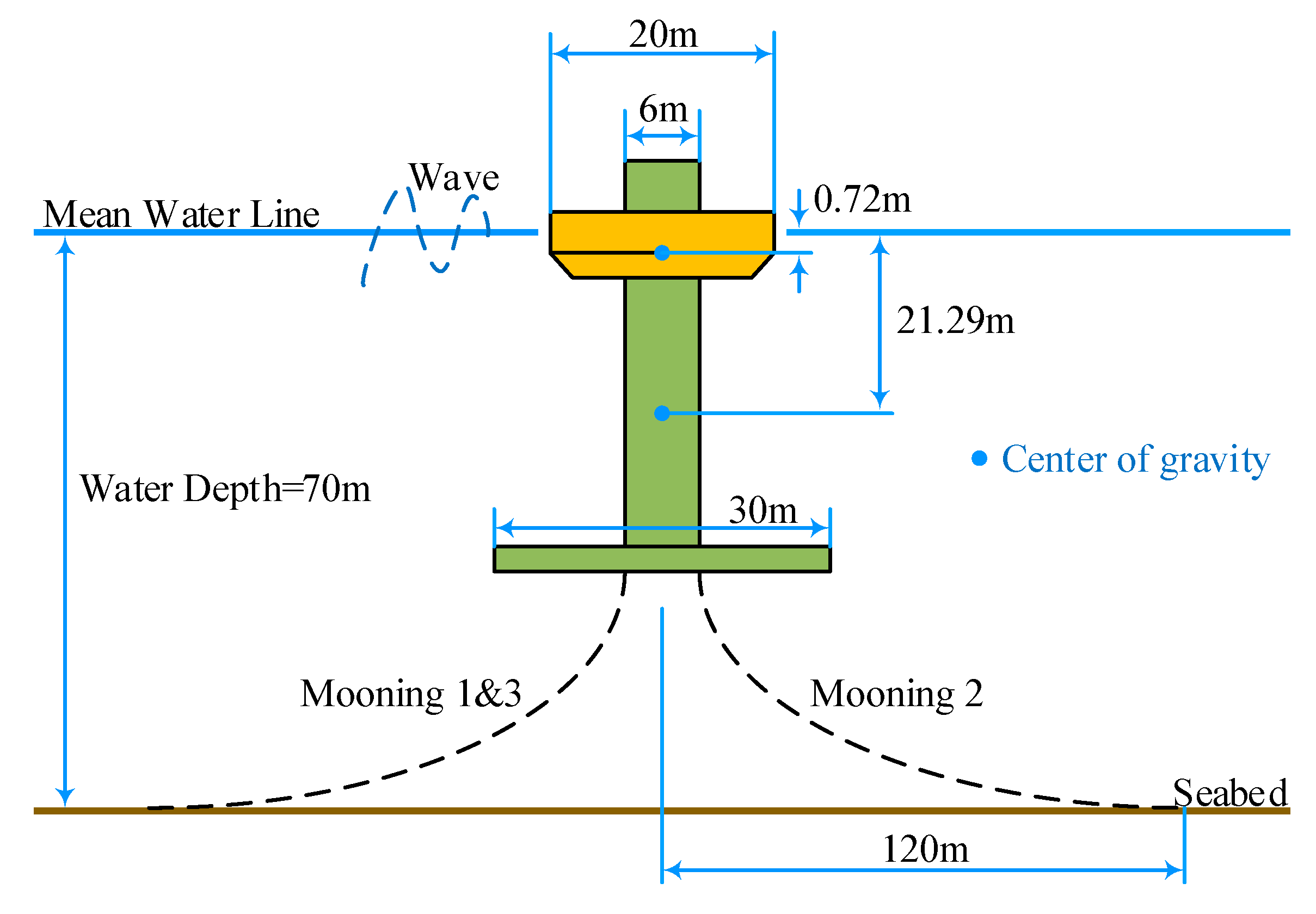
In this paper, a typical double-float point-absorbing wave energy loading device consisting of a float of diameter D1 = 20 m and a spar of diameter D2 = 6 m is used, as shown in Figure 2, which is a double-body pendant-swinging device further designed and developed by the U.S. Department of Energy in the USA on the basis of the PowerBouy device. The spar is fixed to the seabed by three mooring cables in order to limit its vertical motion and prevent it from deviating from its position. The float moves in a pendant motion relative to the spar, which is restrained in all other degrees of freedom by a linear bearing system. A hydraulic system that is powered by the relative motion of the float and the spar realizes the energy conversion. Table 1 displays pertinent parameters like the adopted WEC model’s mass and dimensions. Mahmoodi et al.’s paper [29] provides further in-depth details regarding this device.

2.1. WEC Model

The bottom end of the damping disk in a double-float device is subject to the mooring force, and the float and spar are connected by a power take-off (PTO) system that carries out relative motion in the direction of vertical oscillation to realize energy conversion. The main model for this section is the simplified structure of a coaxial double cylinder. The hydrodynamic properties of the apparatus are examined using linear theory, presuming that the fluid is an ideal, non-viscous, non-spinning, and incompressible fluid. The equations of motion of the floating cylinder and the float in the direction of vertical oscillation can be written as follows using Newton’s second law:
m 1 x ¨ 1 = F e 1 + F h 1 + F PTO + F r a d 11 + F r a d 12
m 2 x ¨ 2 = F e 2 + F h 2 F PTO + F r a d 21 + F r a d 22 + F m
where m 1 and m 2 denote the mass of the float and the float tube, respectively; x ¨ 1 and x ¨ 2 denote the oscillatory acceleration of the float and the float tube, respectively; F e 1 and F e 2 denote the wave excitation force on the float and the float tube, respectively, F PTO denotes the PTO force; F e 1 and F e 2 denote the hydrostatic restoring force on the float and the float tube, respectively; x 1 and x 2 are the oscillatory displacements of the float and the float tube with respect to their hydrostatic equilibrium state; F r a d i j denotes the radial force on float i due to the motion of float j; and F m is the mooring force on the float tube.

2.2. Radiative Force F r a d

The radiation force is the force generated by the action of a radiated wave on a WEC and is calculated in the time domain by using a convolution integral. The formula for the radiation force can be generally expressed as follows:
F r a d ( t ) = A x ¨ ( t ) 0 t K r ( t τ ) x ˙ ( τ ) d τ
where A is the added mass at infinite frequency; K r is the radiative impulse response function; and x ¨ ( t ) and x ˙ ( t ) denote the drooping acceleration and velocity of the WEC, respectively. The additional mass matrix A at infinite frequency is generally written in the following form:
A = [ a 11 a 12 a 1 n a 21 a 22 a 2 n a n 1 a n 2 a n n ]
A is an n × n symmetric matrix, where a i j = a j i , ( i , j ) { 1 , 2 } , n is the number of wave energy devices, i.e., n = 2.
Where there exists a coupled radiative force F r a d i j generated by the interaction force between the floats and the spar,
F r a d 11 = A 11 x ¨ 1 ( t ) + t f r 11 ( t τ ) x ˙ 1 ( τ ) d τ
F r a d 12 = A 12 x ¨ 2 ( t ) + t f r 12 ( t τ ) x ˙ 2 ( τ ) d τ
F r a d 21 = A 21 x ¨ 1 ( t ) + t f r 21 ( t τ ) x ˙ 1 ( τ ) d τ
F r a d 22 = A 22 x ¨ 2 ( t ) + t f r 22 ( t τ ) x ˙ 2 ( τ ) d τ
F r a d i j denotes the radiation force on float i due to the motion of float j; A i j denotes the additional mass at infinite frequency; x ¨ and x ˙ denotes the vertical acceleration and velocity of the device, respectively; and K r denotes the radiation impulse response function.
To improve computational efficiency, a state-space approximation is used to represent the convolution integral term 0 t K r ( t τ ) z ˙ ( τ ) d τ of the radiative force in Equation (2), and the specific details of the derivation of the state-space representation can be found in the work of Kristiansen et al. [30,31,32]. The general formulation is represented by the following equation:
q ˙ ( t ) = A r q ( t ) + B r u ( t )
0 t K r ( t τ ) z ˙ ( τ ) d τ = C r q ( t ) + D r u ( t )
where A r is the system matrix; B r is the input matrix; C r is the output matrix; D r is the feedthrough matrix; and q ( t ) and q ˙ ( t ) are the states of the system and their derivatives, respectively. The input u ( t ) of the system is equal to the velocity term x ˙ ( t ) .

2.3. Hydrostatic Restoring Force F r a d and PTO Force F p t o

The general expression for the hydrostatic restoring force is
F h 1 = g ρ π r 1   2 x 1 ( t ) = K H 1 x 1 ( t )
F h 2 = g ρ π r 2   2 x 2 ( t ) = K H 2 x 2 ( t )
The hydrostatic restoring force F h can be viewed as a linear function of displacement, where ρ is the density of water, g is the acceleration due to gravity, π r 1   2 and π r 2   2 are the projected areas of the submerged volumes of the float and the spar at the surface of the water at hydrostatic water, and K H i is the matrix of hydrostatic stiffness coefficients for the float and the spar.
The PTO system can be simplified to a linear spring-damper system, so the PTO force can be expressed as
F p t o = c p t o ( x ˙ 1 x ˙ 2 ) k p t o ( x 1 x 2 )
where k p t o is the stiffness matrix of the PTO system, c p t o is the damping matrix of the PTO system, and x 1 and x 2 are the displacements of the float and the spar. The stiffness and damping coefficients of the device are set to 0 N/m and 1200 kNs/m, respectively.

2.4. Mooring Force F M

In most of the current studies on excitation estimation strategies for wave energy-generating devices, the mooring force is linearized in the process of motion modeling, but in the real situation, the mooring force of the device is nonlinear. Therefore, in order to be closer to the real situation, nonlinear mooring forces are introduced in the modeling of this paper. The nonlinear mooring force [33] can be expressed as follows:
F m = 3 K n l x 2 ( t ) ( 1 L n l L n l 2 + x 2 ( t ) 2 )
where K n l is the stiffness of the mooring line, L n l is the length of the line, and x 2 is the displacement of the float in the swing direction. In this paper, a three-line mooring is used.
The parameters used for modeling such as additional mass at infinite frequency and hydrodynamic coefficients such as radiation damping coefficients can be obtained from a boundary element software ANSYS AQWA 2021 simulation. Based on the work of Richter et al. [33], the mooring forces are calculated assuming that K n l = 840,000 N/m, L n l = 240 m.

2.5. Modeling the WEC System

The modeling process for the two-body wave energy device takes the form of a state space, and Equations (1)–(3) and (11)–(14) can be expressed as follows:
F PTO + F e 1 K H 1 x 1 A 12 x ¨ 2 m 1 + A 11 = x ¨ 1
F PTO + F e 2 K H 2 x 2 F m ( x ) A 21 x ¨ 1 m 2 + A 22 = x ¨ 2
These equations can be transformed to state-space form by substituting (15) into (16) and vice versa to remove the coupling terms A 21 x 1 and A 12 x 2 . These equations can be reformulated as
x ¨ 1 ( m 1 + A 11 A 12 A 21 m 2 + A 22 M c 1 ) = ( c PTO A 12 m 2 + A 22 + c PTO ) x ˙ 1 + ( c PTO + A 12 c PTO m 2 + A 22 ) x ˙ 2 ( k PTO A 12 m 2 + A 22 + k PTO + K H 1 ) x 1 + ( k PTO + A 12 ( k PTO + K H 2 ) m 2 + A 22 ) x 2 + F e 1 A 12 m 2 + A 22 F e 2 + A 12 m 2 + A 22 F m
x ¨ 2 ( m 2 + A 22 A 21 A 12 m 1 + A 11 M c 2 ) = ( c PTO + A 21 c PTO m 1 + A 11 ) x ˙ 1 = ( c PTO A 21 m 1 + A 11 + c PTO ) x ˙ 2 + ( k PTO + ( k PTO + K H 1 ) A 21 m 1 + A 11 ) x 1 ( k PTO A 21 m 1 + A 11 + k PTO + K H 2 ) x 2 A 21 m 1 + A 11 F e 1 + F e 2 F m
The state vector of the nonlinear state-space model is x ˙ = [ x 1 x 2 x ˙ 1 x ˙ 2 ] T , and the initial condition is x ˙ ( 0 ) = [ 0 0 0 0 ] T . The nonlinear system modeled can thus be expressed as
x ˙ = F x + B 1 F e x c + B 2 F m + B 3 F r a d c
where
F = [ 0 0 1 0 0 0 0 1 1 M e 1 ( k PTO A 12 M 2 K p 1 ) 1 M e 1 ( k PTO + A 12 K p 2 M 2 ) 1 M e 1 ( c PTO A 12 M 2 c PTO ) 1 M e 1 ( c PTO + c PTO A 12 M 2 ) 1 M e 2 ( k PTO + A 21 K p 1 M 1 ) 1 M e 2 ( k PTO A 21 M 1 + K p 2 ) 1 M e 2 ( c PTO + c PTO A 21 M 1 ) 1 M e 2 ( c PTO A 21 M 1 + c PTO ) ]
B 1 = [ 0 0 0 0 1 M e 1 A 12 M e 1 M 2 A 21 M e 2 M 1 1 M e 2 ]
B 2 = [ 0 0 A 12 M e 1 M 2 1 M e 2 ]
B 3 = [ 0 0 0 0 1 0 0 1 ]
where
M i = m i + A i i , i { 1 , 2 }
K P i = k PTO + K H i , i { 1 , 2 }

3. Methods

3.1. Kalman Filter Estimation

There are numerous extensions and modifications available for the Kalman filter approach, which is a very popular tool for wave excitation force estimation. The extended Kalman filter is one of the most often used modified Kalman filter algorithms available today. When the nonlinear factor is smooth, evolves slowly with respect to the discrete time step, and is unaffected by time delays, the extended Kalman filter works well. Because of these limitations, the extended Kalman filter is typically one of the best options for handling linearized problems in nonlinear WEC models.
The fundamental idea behind the EKF-based estimator is to see the wave excitation force as a dynamic system state. It is assumed that the dynamical system is a constant-frequency resonator model since the excitation force is intrinsically oscillatory [34]. The filter algorithm with a linear model and tiny time step maintains a relatively small deviation from the nonlinear model. In essence, this model is linearized around the estimate of the final state at every discrete time step. As a result, the system matrix is no longer constant but instead changes with each time step of the Kalman filtering process, which uses the time step of the most recent estimated system state as Fk−1.
The dynamic system of the WEC with a sampling period (Ts) of 0.05 s is described as follows:
x ˙ ( k ) = f ( x k 1 , u k 1 , w k 1 )
y ( k ) = H x ( k ) + ν ( k )
The process model (26) defines the state of the system from ( k 1 ) T s to k T s . f is a function representing the state of the nonlinear system, B is the control input matrix used for the control vector F r a d ( k 1 ) , and w k 1 is the process noise vector assumed to be a zero-mean Gaussian with covariance Q, i.e., w k 1 ~ N ( 0 , Q ) . The measurement model (27) describes the relationship between the system state x ( k ) and the measured values y ( k ) . The measurement vector contains the displacements and velocities of the WEC. H is the observation matrix, and ν ( k ) is the zero-mean Gaussian measurement noise vector assumed to have covariance R, i.e., ν ( k ) ~ N ( 0 , R ) .
The Kalman filter estimates the state of the system by cycling through the steps of gain, time update, and state update at each discrete time. The extended Kalman filter algorithm is represented by the prediction and update equations as follows:
Time to update:
x ^ k | k 1 = f ( x k 1 , u k 1 , w k 1 )
P k | k 1 = A k P k 1 + A k T + W k Q W k T
Status updates:
K k = P k | k - 1 H k T ( H k P k | k - 1 H k T + V k R V k T ) 1
x ^ k + = x ^ k | k 1 + K k ( z k H k T x ^ k | k 1 )
P k + = ( I K k H k ) P k | k 1
The symbol ^ denotes the estimate, the superscript symbols − and + denote the a priori and a posteriori estimates, the superscript symbol T denotes the transpose, I is the unit matrix, P denotes the state error covariance matrix, and K denotes the Kalman gain. The state vector x _ ˙ consists of the droop displacement, droop velocity, and wave excitation force and their derivatives at each frequency:
x ˙ = [ x 1 x 2 x ˙ 1 x ˙ 2 F e 1 F e 2 F ˙ e 1 F ˙ e 2 ] T
where F e i and F ˙ e i are described as follows:
F e x = [ F e x c 11 F e x c 21 F e x c 12 F e x c 22 F e x c 1 f F e x c 2 f ]
F ˙ e x = [ F ˙ e x c 11 F ˙ e x c 21 F ˙ e x c 12 F ˙ e x c 22 F ˙ e x c 1 f F ˙ e x c 2 f ]
F e x c i j and F ˙ e x c i j are the excitation forces acting on the WEC and their derivatives. i { 1 , 2 } , j { 1 , , f } , f is the number of frequencies of the excitation force used for modeling.
The state vector of the nonlinear state-space model is x ˙ = [ x 1 x 2 x ˙ 1 x ˙ 2 F e 1 F e 2 F ˙ e 1 F ˙ e 2 ] T , and the initial condition is  x ˙ ( 0 ) = [ 0 0 0 0 0 0 0 0 ] T . The model can be expressed as
x ˙ = A n l x + l ( x ) + B F r a d c
where the state transfer matrix A is
A n l = [ 0 2 × 2 I 2 × 2 0 2 × 2 f 0 2 × 2 f F 1 F 2 M 2 × 2 f 0 2 × 2 f 0 2 f × 2 0 2 f × 2 0 2 f × 2 f I 2 f × 2 f 0 2 f × 2 0 2 f × 2 Ω 2 0 2 f × 2 f ]
where
M = [ M M ] f
M = [ 1 M e 1 A 12 M e 1 M 2 A 21 M e 2 M 1 1 M e 2 ]
Since the wave excitation force is assumed to be the superposition of many sinusoids of different phases and amplitudes, the second-order derivative of the wave excitation force at each frequency is
F ¨ e x c i j = ω j 2 F e x c i j
Thus, the diagonal matrix Ω at different frequencies can be expressed as follows:
Ω = [ ω 1 I 2 × 2 0 2 × 2 0 2 × 2 0 2 × 2 ω 2 I 2 × 2 0 2 × 2 0 2 × 2 0 2 × 2 ω f I 2 × 2 ]
The nonlinear term l ( x ) and the control input matrix B are denoted as
l ( x ) = [ 0 2 × 1 3 K n l A 12 M e 1 M 2 ( 1 L n l L n l 2 + x 2 2 ) x 2 3 K n l M e 2 ( 1 L n l L n l 2 + x 2 2 ) x 2 0 4 f × 1 ]
B = [ 0 2 × 2 I 2 × 2 0 4 f × 2 ]

3.2. Discretization

Finite parameterizations of controls and constraints are widely employed in many recent works to solve optimization issues directly. As a result, the system needs to be represented as the following kind of discrete nonlinear state-space model [33]:
x k + 1 = f k ( x k , u k , s k )
The function f maps the current state x k , controllable input u k , and uncontrollable input s k to the next state x k + 1 of the system. A nonlinear system x ˙ = f ( x ( t ) ) + g ( x ( t ) ) u ( t ) can be discretized by approximating the representation of the sampled data, i.e.,
x k + 1 = x k + l = 1 M A [ l ] ( x k , u k ) h l l !
where
A [ l + 1 ] ( x , u ) = δ A [ l ] ( x , u ) δ x ( f ( x ) + g ( x ) u ) l { 1 , 2 , 3 , , M }
where M denotes the order of discretization and h denotes the sampling interval. In this paper, the second-order discretization is used, i.e., M = 2. For the nonlinear system (37)–(43), it follows that
A [ 1 ] = A n l x + l ( x ) + B u
A [ 2 ] = [ A n l + l ( x ) ] [ A n l x + l ( x ) + B u ]
According to Equation (45), the discrete system can be expressed as
x k + 1 = A n l , d 1 x k + A n l , d 2 l ( x k ) + h 2 2 l k ( x k ) A n l x k + h 2 2 l ( x k ) l ( x k ) + B d u + l ( x k ) B u
where
A n l , d 1 = I + h A n l + h 2 2 A n l 2
A n l , d 2 = h I + h 2 2 A n l
B d = h B + h 2 2 A n 1 B
l k ( x k ) = [ 0 2 × 1 0 2 × 1 0 2 × 1 0 3 K n l A 12 M e 1 M 2 ( 1 L 3 n l ( L n l 2 + x 2 2 ) 1.5 ) 0 1 × ( 4 f + 2 ) 0 3 K n l M e 2 ( 1 L 3 n l ( L n l 2 + x 2 2 ) 1.5 ) 0 1 × ( 4 f + 2 ) 0 4 f × 1 0 4 f × 1 0 4 f × ( 4 f + 2 ) ]

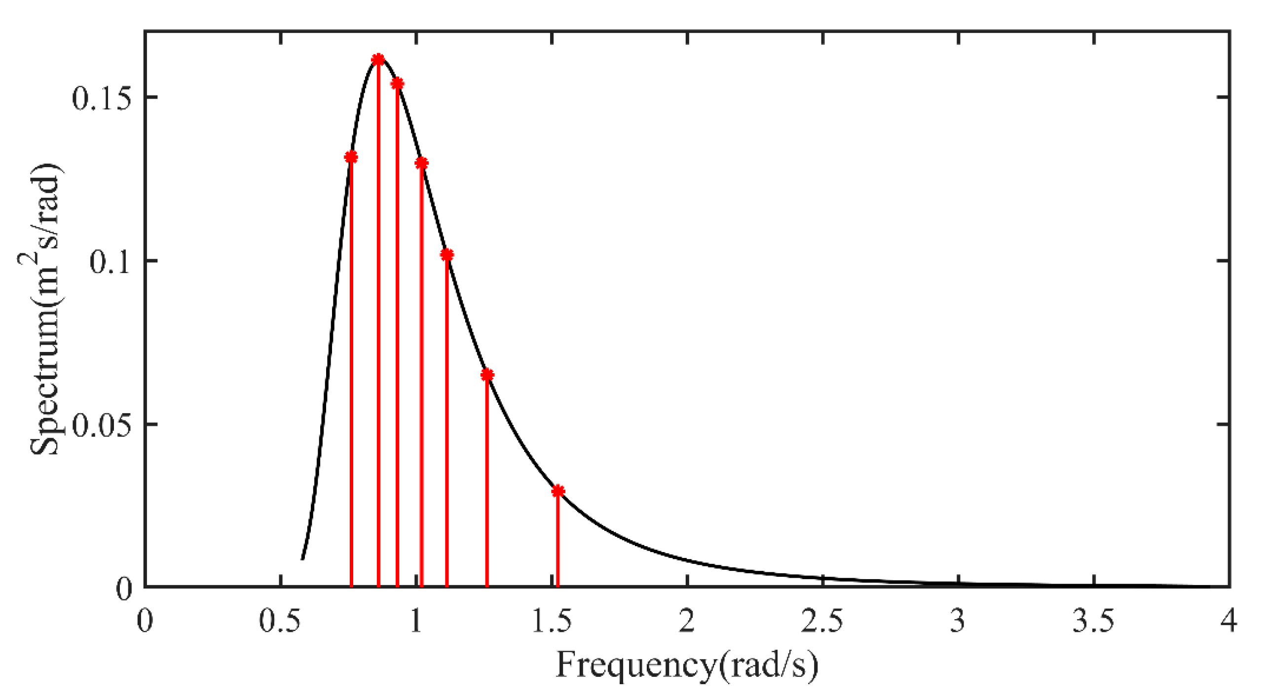
3.3. Equal-Energy Method

The use of the EKF requires that the wave excitation force be considered as a state of the moving system, and the frequencies required in the resonator model representing the excitation force can be obtained from the predetermined wave spectrum by the equal-energy method.
The equal-energy method, which requires equal-energy spectral areas for each wave frequency, is now widely used in the study of irregular wave delineation [35,36]. In addition to this, the equal-frequency resolution method [37,38] is widely used for irregular waves. The former is used in this paper. Most of the current equal-energy methods use 5 or 7 frequency values to divide the energy spectrum, so 7 frequency values are used here for the time being. Figure 3 represents the energy spectrum divided by the equal-energy method for seven frequencies, the vertical red lines indicate the division between each equal-energy region of the spectrum, and the red circles indicate the power and frequency of the components chosen to form the perturbation equation. The effect of the number of frequency divisions on the estimation accuracy of the excitation estimator is described in detail in Section 4.

4. Results and Discussion

In this paper, we use the Goodness of Fit (GoF) to characterize the accuracy of the WEC incentive estimation; GoF is given as follows [39]:
GoF = [ 1 k = 1 N ( f k f ^ k ) 2 k = 1 N f k 2 ] × 100 %
where f k and f ^ k are the true and estimated values at moment k, respectively, and N is the number of estimates.

4.1. The Effect of Random Phase on the Estimation Results

The amplitude of the wave is given by the PM spectrum, with a meaningful wave height (H) of 1.25 m and a peak period (T) of 7.25 s. In order to evaluate the model in different sea states, it is necessary to randomly generate multiple sets of phase-simulated irregular waves in several simulation runs to obtain the average GoF value [39].
In this work, 40 simulations were run for a particular estimator; that is, 40 distinct wave phases were employed to model irregular waves. The correlation between the number of runs and the 95% confidence intervals for the float and the spar, respectively, is shown in Figure 4 and Figure 5. The blue bar graphs indicate the average GoF values obtained for a given estimator for the different number of simulations performed, and the red error bars indicate the 95% confidence intervals for the set of samples to measure the stability of the experimental data. The average GoF values produced when the number of simulation runs is less are found to be much lower than the stable value when comparing the GoF curves of the spar and the float. However, after 15 simulations, they begin to gradually converge as the number of simulation runs increases. After 26 runs, the average GoF values show a tendency to stabilize. After 26 simulations, the float’s GoF values converge to approximately 84%, whereas the spar’s GoF values converge to approximately 84.3%. At this moment, a half-width of 0.25% of the mean value corresponds to a 95% confidence interval. In other words, the average GoF estimate derived from 26 simulations can be used for further work, and there is a 95% chance that the real value will fall within ±0.25% of the estimated average GoF value.

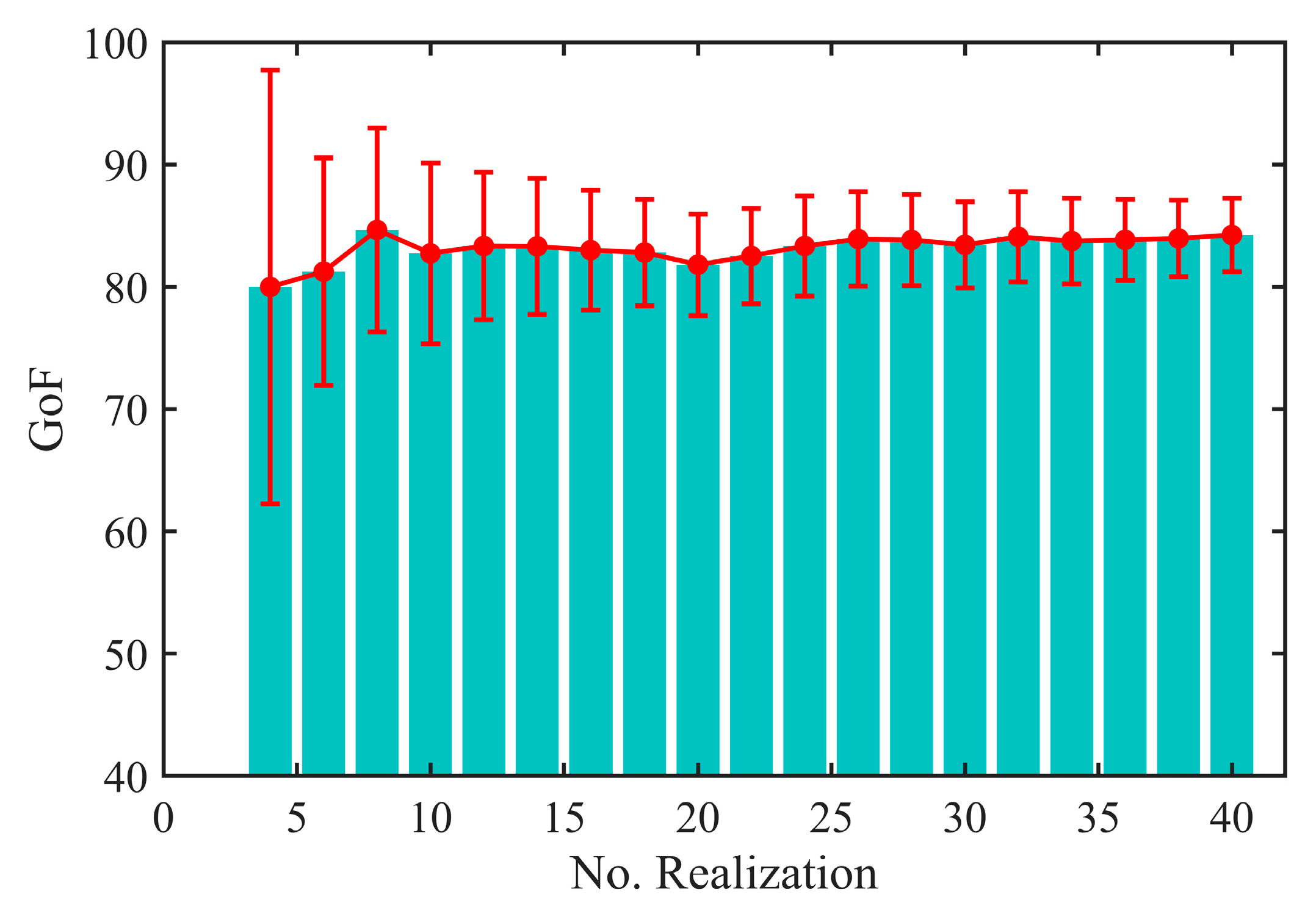
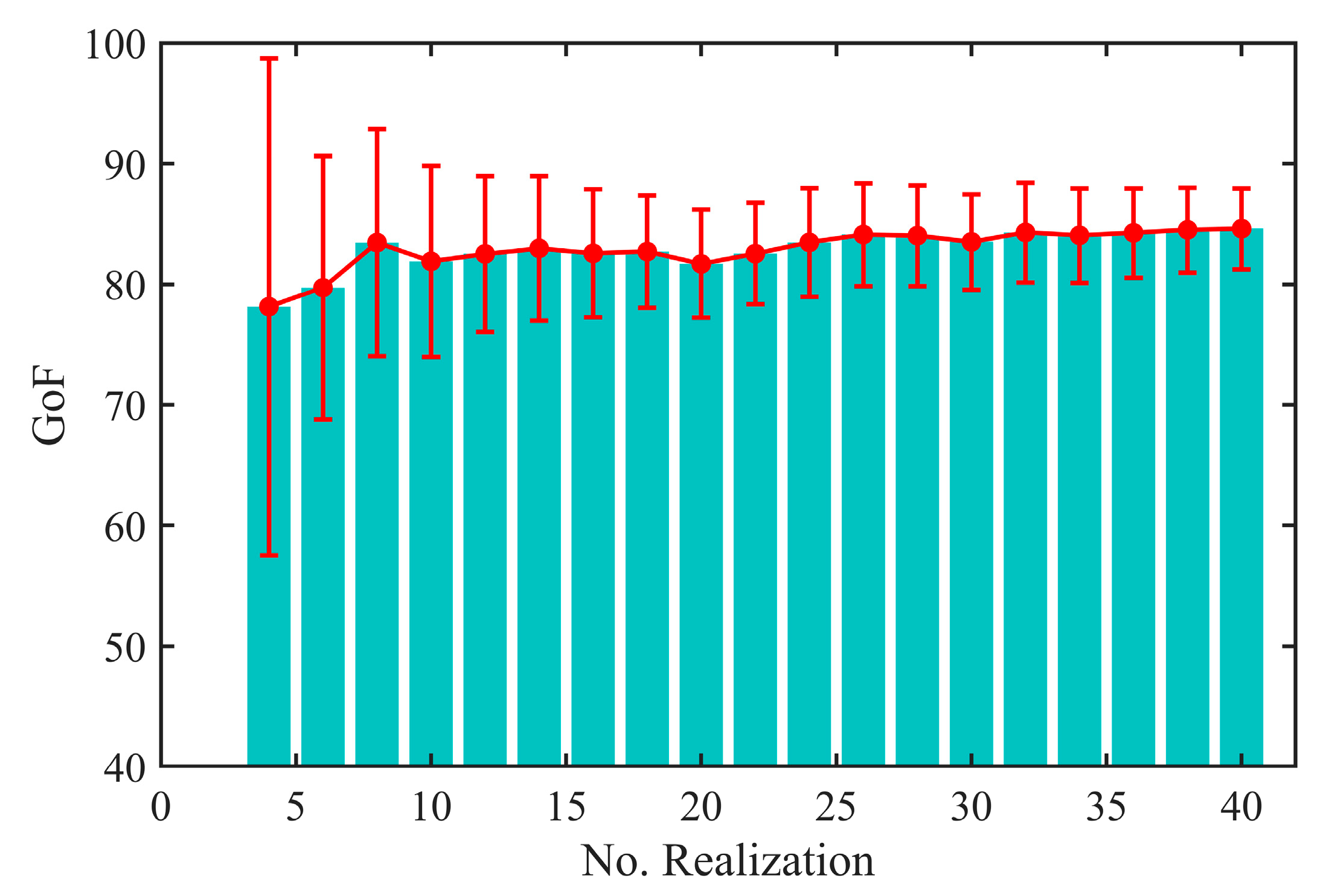
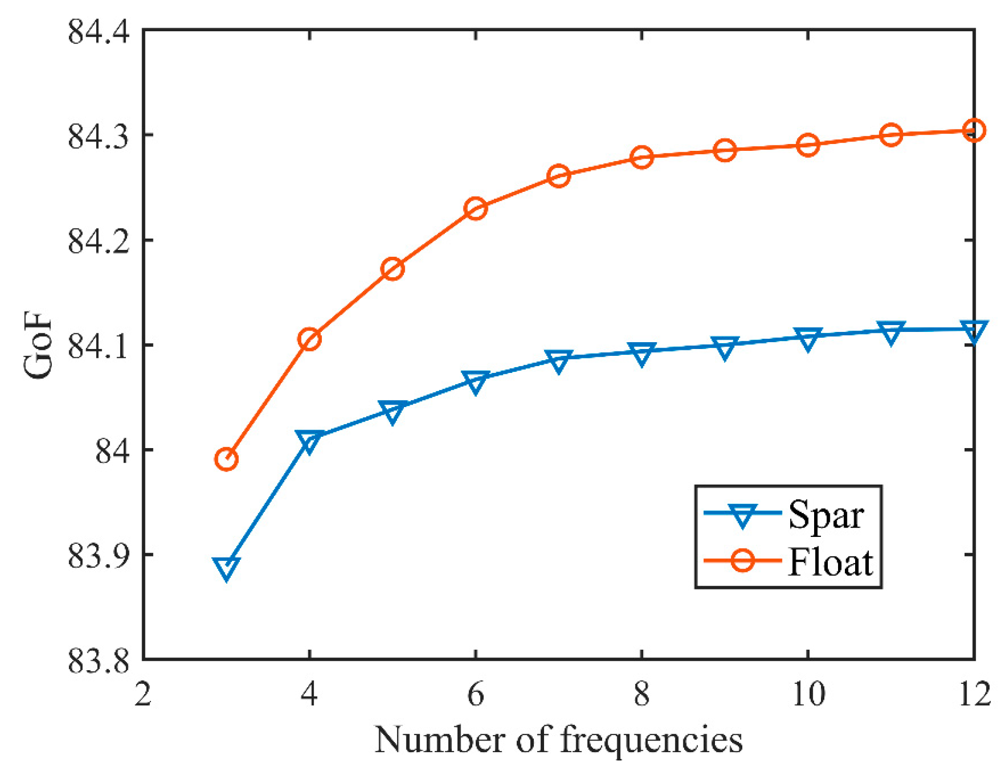
4.2. Impact of Dividing the Number of Frequencies on the Estimation Results

In the current study, five or seven frequencies are generally used, with the values selected by employing a mixture of frequencies, thereby offering the best estimation accuracy. The ideal number of frequencies and their values depend on the actual sea state. In actuality, frequencies can be chosen from the wave spectrum forecast by meteorological organizations and modified in response to changes in the sea state.
The wave spectrum is divided into 499 bins of equal energy content by 500 wave frequencies using the default spectral binning approach of WEC-Sim [40]. Wave forces are therefore only estimated on each of the 500 wave frequencies when utilizing the equal-energy method. By lowering the number of frequencies at which the wave train is defined and, consequently, the number of frequencies at which the wave force is computed, the equal-energy formulation expedites the irregular wave simulation time. It stops segments with extremely low energies from being generated, which would require extra computing power.
The effect of the number of divisions of frequencies in the equal-energy method on the estimation accuracy is shown in Figure 6. From the figure, it can be found that the estimation accuracy gradually becomes higher as the number of frequency selections increases. At seven frequencies, the average GoF value of the float reaches 84.07%, and the average GoF value of the spar reaches 84.26%. However, for every increase in the number of frequencies, the system matrix A increases by two rows and two columns; i.e., an excessive number of frequencies will seriously reduce the computational speed and affect the efficiency of the estimation. It can be seen from Figure 6 that after the number of frequencies reaches seven, the rising speed of estimation accuracy decreases significantly, the growth trend of GoF value tends to stabilize gradually, and the sensitivity of estimation accuracy to the number of frequencies decreases. Therefore, selecting seven frequencies for estimation is a suitable choice. As shown in Figure 7 and Figure 8 for the excitation estimation of the float and the spar when the number of frequencies is seven, the red curve is the estimation result, and the blue dashed line is the real value expressed in terms of the WEC-Sim running results. It can be found that the estimation results obtained with seven frequencies are fitted more satisfactorily to the real values.

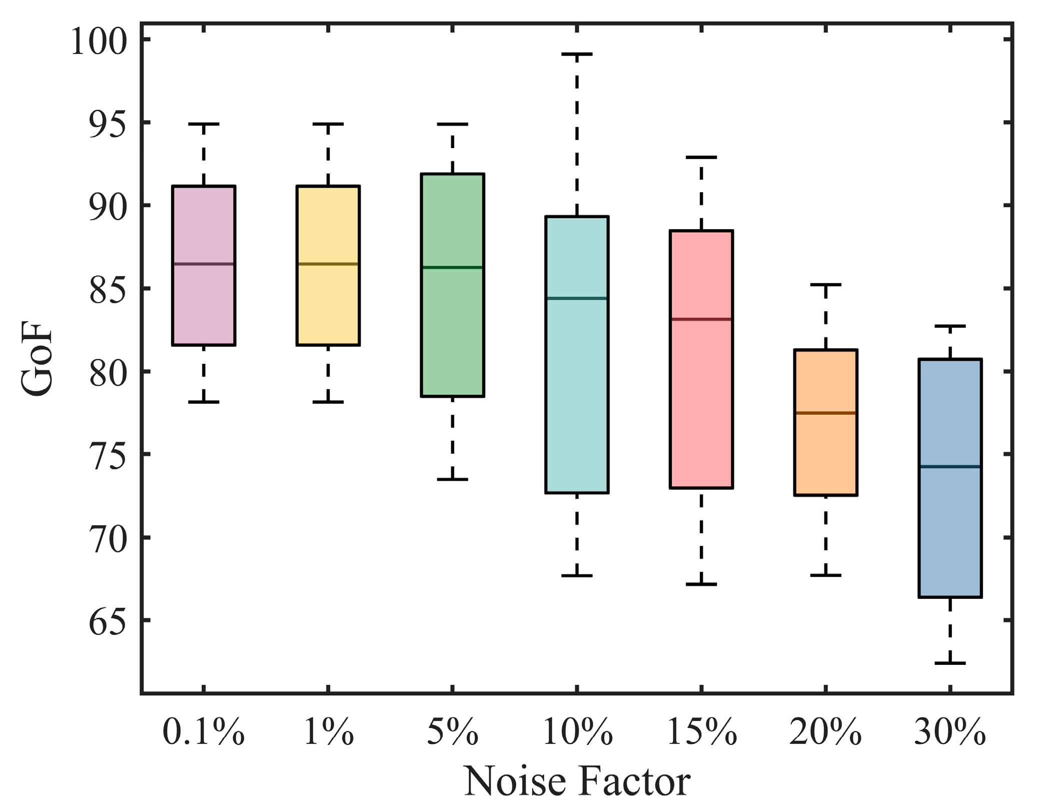
4.3. Effect of Noise Factor on Estimation Results

Artificial zero-mean Gaussian noise is introduced into the measurement procedure in order to examine the susceptibility of the EKF estimation algorithm to measurement noise. The excitation estimation results for the spar and the float derived from 26 simulations with varying noise factors are shown in Figure 9 and Figure 10, respectively. With a significant rise in the noise factor, the excitation estimation accuracies of the spar and the float in the figures both decline, while the overall % drop is not particularly high. The float’s GoF value is 86.82% when the noise factor is assumed to be 0.1% of the WEC kinematic response. The GoF value of the float drops to 71.37% when the noise factor value is raised to 30% of the WEC kinematic response. In contrast, the GoF value of the spar is 87.31% when the noise factor is assumed to be 0.1% of the WEC kinematic response, and it drops to 74.25% when the noise factor is increased to 30% of the WEC kinematic response. Overall, there is not much of a drop in the float and spar’s excitation estimation accuracy, suggesting that measurement noise has a negligible impact on wave excitation estimation.
By comparing Figure 9 and Figure 10, it is possible to determine that the spar’s GoF value changed less than that of the float under the same measurement noise. This suggests that the float’s estimation result is less accurate than the spar’s under the same measurement noise because the spar’s estimation accuracy is less affected by the measurement noise. That is, the spar has superior stability compared to the float and is less impacted by the noise under the effect of nonlinear mooring force as measurement noise increases. As a result, a float subjected to the mooring force has greater measurement accuracy and stability than a float not exposed to the mooring force in the event of significant measurement noise. Furthermore, the measurement noise in the real world is actually far less than the synthetic noise used in the simulation, as confirmed by the work of Davis et al. [36] and Bosma et al. [41].

5. Conclusions

This paper presents a method for constructing a wave excitation force estimator using the extended Kalman filter method for nonlinear WEC systems, where highly nonlinear mooring forces are considered. The estimator models the wave excitation force as a resonator consisting of sinusoidal waves of a specific frequency, which is determined using the isoenergetic method. In this work, the effects of the random phase and the number of frequencies of the resonators on the average GoF value are analyzed in detail.
In this work for a given estimator, 40 different wave phases are used to simulate irregular waves. As the number of simulations increases, the average GoF value obtained after 26 simulations stabilizes and results in a 95% confidence interval with a half-width of 0.25% of the mean value. That is, follow-up work can be performed with the estimated mean GoF obtained from 26 simulations, and the probability that the actual mean GoF is within ±0.25% of the estimated mean GoF will reach 95%.
The use of the EKF requires that the wave excitation force be considered as a state of the moving system, and the frequencies required in the resonator model representing the excitation force can be obtained from the predetermined wave spectrum by the isoenergetic method. In this work, the effect of the number of divisions of frequencies in the equal-energy method on the estimation accuracy is analyzed. The estimation accuracy becomes progressively higher as the number of frequency selections increases. After the number of frequencies reaches seven, the rate of the increase in the estimation accuracy decreases significantly, and the growth trend of the GoF value tends to level off gradually. Considering that too high a number of frequencies will seriously reduce the computational speed and affect the efficiency of estimation, it is a more appropriate choice to select seven frequencies for estimation.
In addition, the effect of measurement noise on the estimation accuracy is evaluated, and the negative correlation between the measurement noise and the estimation accuracy is analyzed and obtained. The effect of measurement noise on the accuracy of estimating the wave excitation force for the float and spar of the dual-float device is similar. As the measurement noise increases, the accuracy of estimating the wave excitation of the float and spar decreases.
This work demonstrates that the extended Kalman filter estimation algorithm used can provide experimental data of the excitation force with high estimation accuracy and that the resonator model of the wave excitation force used in the algorithm is a realistic mechanical model. In practical engineering applications, the mooring systems of the devices are mostly nonlinear. And this work shows that it is possible to accurately estimate the wave excitation force for nonlinear systems by using an extended Kalman filter, thus providing more accurate data information for WEC deployment and control strategies. And in real scenarios, further studies are needed to verify the superiority of the proposed method in WECs; e.g., viscous drag needs to be considered.

Author Contributions

Y.Z., conceptualization, methodology, writing—editing, software; Z.Z., J.W. and J.Q., validation and investigation; S.H., data curation and editing. G.X., software and formal analysis. Y.L., reviewing and supervision. All authors have read and agreed to the published version of the manuscript.

Funding

This research was funded by the National Natural Science Foundation of China, 52171265, U22A20242.

Data Availability Statement

Data are contained within the article.

Conflicts of Interest

The authors declare no conflicts of interest.

References

  1. Feng, S.; Li, F. Introduction to Marine Science; Higher Education Press: Beijing, China, 2006; p. 185. [Google Scholar]
  2. Mork, G.; Barstow, S.; Kabuth, A.; Pontes, M.T. Assessing the global wave energy potential. In Proceedings of the ASME 29th International Conference on Ocean, Offshore and Arctic Engineering, OMAE, Shanghai, China, 6–11 June 2010. [Google Scholar]
  3. IEA. Data and Statistics: Electricity[DB/OL]. Available online: https://www.iea.org (accessed on 12 February 2022).
  4. Gao, D.; Wang, F.; Shi, H.; Chang, Z.; Zhao, L. Research Progress of Wave Energy Generators in Foreign Countries. Ocean. Dev. Manag. 2012, 29, 21–26. [Google Scholar]
  5. Wang, Z.; Zhou, L.; Dong, S.; Wu, L.; Li, Z.; Mou, L.; Wang, A. Wind wave characteristics and engineering environment of the South China Sea. J. Ocean. Univ. China 2014, 13, 893–900. [Google Scholar] [CrossRef]
  6. Han, B.; Chu, J.; Xiong, Y.S.; Yao, F. Progress of Research on Ocean Wave Energy Power Generation. Power Syst. Clean Energy 2012, 28, 61–66. [Google Scholar]
  7. López, I.; Andreu, J.; Ceballos, S. Review of wave energy technologies and the necessary power-equipment. Renew. Sustain. Energy Rev. 2013, 27, 413–434. [Google Scholar] [CrossRef]
  8. Clément, A.; McCullen, P.; Falcão, A.; Fiorentino, A.; Gardner, F.; Hammarlund, K.; Lemonis, G.; Lewis, T.; Nielsen, K.; Petroncini, S.; et al. Wave energy in Europe: Current status and perspectives. Renew. Sustain. Energy Rev. 2002, 6, 405–431. [Google Scholar] [CrossRef]
  9. Wang, C.; Lu, W. Ocean Energy Resource Analysis Methodology and Reserve Assessment; Ocean Press: Beijing, China, 2009; pp. 106–129. [Google Scholar]
  10. Wang, L.; Isberg, J.; Tedeschi, E. Review of control strategies for wave energy conversion systems and their validation: The wave-to-wire approach. Renew. Sustain. Energy Rev. 2018, 81, 366–379. [Google Scholar] [CrossRef]
  11. Rusu, L.; Onea, F. The performance of some state-of-the-art wave energy converters in locations with the worldwide highest wave power. Renew. Sustain. Energy Rev. 2017, 75, 1348–1362. [Google Scholar] [CrossRef]
  12. Pena-Sanchez, Y.; Windt, C.; Davidson, J.; Ringwood, J.V. A critical comparison of excitation force estimators for wave-energy devices. IEEE Trans. Control. Syst. Technol. 2020, 28, 2263–2275. [Google Scholar] [CrossRef]
  13. Guo, B.; Patton, R.J.; Jin, S. Numerical and experimental studies of excitation force approximation for wave energy conversion. Renew. Energy 2018, 125, 877–889. [Google Scholar] [CrossRef]
  14. Abdelkhalik, O.; Zou, S.; Bacelli, G.; Robinett, R.D.; Wilson, D.G.; Coe, R.G. Estimation of excitation force on wave energy converters using pressure measurements for feedback control. In Proceedings of the OCEANS 2016 MTS/IEEE Monterey, OCE, Monterey, CA, USA, 19–23 September 2016. [Google Scholar]
  15. Gao, J.; He, Z.; Zang, J.; Chen, Q.; Ding, H.; Wang, G. Numerical investigations of wave loads on fixed box in front of vertical wall with a narrow gap under wave actions. Ocean Eng. 2020, 206, 107323. [Google Scholar] [CrossRef]
  16. Gao, J.; Lyu, J.; Wang, J.; Zhang, J.; Liu, Q.; Zang, J.; Zou, T. Study on Transient Gap Resonance with Consideration of the Motion of Floating Body. China Ocean. Eng. 2022, 36, 994–1006. [Google Scholar] [CrossRef]
  17. Fusco, F.; Ringwood, J.V. Short-term wave forecasting for real-time control of wave energy converters. IEEE Trans. Sustain. Energy 2010, 1, 99–106. [Google Scholar] [CrossRef]
  18. Paparella, F.; Monk, K.; Winands, V.; Lopes, M.F.P.; Conley, D.; Ringwood, J.V. Up-wave and autoregressive methods for short-term wave forecasting for an oscillating water column. IEEE Trans. Sustain. Energy 2015, 6, 171–178. [Google Scholar] [CrossRef]
  19. Merigaud, A.; Ringwood, J.V. Incorporating ocean wave spectrum information in short-term free-surface elevation forecasting. IEEE J. Ocean. Eng. 2019, 44, 401–414. [Google Scholar] [CrossRef]
  20. Ma, Y.; Sclavounos, P.D.; Cross-Whiter, J.; Arora, D. Wave forecast and its application to the optimal control of offshore floating wind turbine for load mitigation. Renew Energy 2018, 128, 163–176. [Google Scholar] [CrossRef]
  21. Ali, M.; Prasad, R. Significant wave height forecasting via an extreme learning machine model integrated with improved complete ensemble empirical mode decomposition. Renew. Sustain. Energy Rev. 2019, 104, 281–295. [Google Scholar] [CrossRef]
  22. Desouky, M.A.A.; Abdelkhalik, O. Wave prediction using wave rider position measurements and NARX network in wave energy conversion. Appl. Ocean Res. 2019, 82, 10–21. [Google Scholar] [CrossRef]
  23. Mahmoodi, K.; Nepomuceno, E.; Razminia, A. Wave excitation force forecasting using neural networks. Energy 2022, 247, 123322. [Google Scholar] [CrossRef]
  24. Abdelkhalik, O.; Zou, S.; Robinett, R.; Bacelli, G.; Wilson, D. Estimation of excitation forces for wave energy converters control using pressure measurements. Int. J. Control 2016, 90, 1793–1805. [Google Scholar] [CrossRef]
  25. Brekken, T.K.A. On model predictive control for a point absorber wave energy converter. In Proceedings of the 2011 IEEE Trondheim PowerTech, Trondheim, Norway, 19–23 June 2011. [Google Scholar]
  26. Ling, B.A. Real-Time Estimation and Prediction of Wave Excitation Forces for Wave Energy Control Applications. In Proceedings of the ASME 2015 34th International Conference on Ocean, Offshore and Arctic Engineering, St. John’s, NL, Canada, 31 May–5 June 2015. [Google Scholar]
  27. Nguyen, H.-N.; Tona, P. Wave Excitation Force Estimation for Wave Energy Converters of the Point-Absorber Type. IEEE Trans. Control. Syst. Technol. 2018, 26, 2173–2181. [Google Scholar] [CrossRef]
  28. Abril, M.G.; Paparella, F.; Ringwood, J.V. Excitation force estimation and forecasting for wave energy applications. In International Federation of Automatic Control; Elsevier: Amsterdam, The Netherlands, 2017; pp. 14692–14697. [Google Scholar]
  29. Mahmoodi, K.; Ghassemi, H.; Razminia, A. Performance assessment of a two-body wave energy converter based on the Persian Gulf wave climate. Renew. Energy 2020, 159, 519–537. [Google Scholar] [CrossRef]
  30. Yu, Z.; Falnes, J. State-space modelling of a vertical cylinder in heave. Appl. Ocean Res. 1995, 17, 265–275. [Google Scholar]
  31. Kristiansen, E.; Hjulstad, Å.; Egeland, O. State-space representation of radiation forces in time-domain vessel models. Ocean Eng. 2005, 32, 2195–2216. [Google Scholar] [CrossRef]
  32. Taghipour, R.; Perez, T.; Moan, T. Hybrid frequency–time domain models for dynamic response analysis of marine structures. Ocean Eng. 2008, 35, 685–705. [Google Scholar] [CrossRef]
  33. Richter, M.; Magana, M.E.; Sawodny, O.; Brekken, T.K.A. Nonlinear Model Predictive Control of a Point Absorber Wave Energy Converter. IEEE Trans. Sustain. Energy 2013, 4, 118–126. [Google Scholar] [CrossRef]
  34. Bonfanti, M.; Hillis, A.; Sirigu, S.A.; Dafnakis, P.; Bracco, G.; Mattiazzo, G.; Plummer, A. Real-Time Wave Excitation Forces Estimation: An Application on the ISWEC Device. J. Mar. Sci. Eng. 2020, 8, 825. [Google Scholar] [CrossRef]
  35. Yerai, S.P.; Marina, A.G.; Francesco, P.; Ringwood, J.V. Estimation and Forecasting of Excitation Force for Arrays of Wave Energy Devices. IEEE Trans. Sustain. Energy 2018, 9, 1672–1680. [Google Scholar]
  36. Davis, A.F.; Fabien, B.C. Wave excitation force estimation of wave energy floats using extended Kalman filters. Ocean. Eng. 2020, 198, 106970. [Google Scholar] [CrossRef]
  37. Gao, J.; Chen, H.; Zang, J.; Chen, L.; Wang, G.; Zhu, Y. Numerical investigations of gap resonance excited by focused transient wave groups. Ocean. Eng. 2020, 212, 107628. [Google Scholar] [CrossRef]
  38. Gao, J.; Ma, X.; Zang, J.; Dong, G.; Ma, X.; Zhu, Y.; Zhou, L. Numerical investigation of harbor oscillations induced by focused transient wave groups. Coast. Eng. 2020, 158, 103670. [Google Scholar] [CrossRef]
  39. Zhang, Z.; Qin, J.; Wang, D.; Wang, W.; Liu, Y.; Xue, G. Research on wave excitation estimators for arrays ofwave energy converters. Energy 2023, 264, 126133. [Google Scholar] [CrossRef]
  40. Kazantzis, N.; Chong, K.T.; Park, J.H.; Parlos, A.G. Control-relevant discretization of nonlinear systems with time-delay using taylor-lie series. J. Dyn. Sys. Meas. Control 2005, 127, 153–159. [Google Scholar] [CrossRef]
  41. Bosma, B.; Thiebaut, F.; Sheng, W. Comparison of a catenary and compliant taut mooring system for marine energy systems. In Proceedings of the 11th European Wave and Tidal Energy Conference (EWTEC2015), Nantes, France, 6–11 September 2015. [Google Scholar]
Figure 1. Schematic diagram of the technical route.
Energies 17 00704 g001
Figure 2. Schematic diagram of a floating wave energy device model with three-line mooring.
Energies 17 00704 g002
Figure 3. Equal-energy method.
Energies 17 00704 g003
Figure 4. Relationship between different numbers of simulations and the average GoF value of the float. The blue bar indicate the average GoF values. The 95% confidence intervals are denoted with the red error bars.
Energies 17 00704 g004
Figure 5. Relationship between different numbers of simulations and the average GoF value of the spar.
Energies 17 00704 g005
Figure 6. Excitation estimation accuracy of the device for different numbers of frequencies.
Energies 17 00704 g006
Figure 7. Estimation of float excitation for 7 frequencies.
Energies 17 00704 g007
Figure 8. Estimation of spar excitation for 7 frequencies.
Energies 17 00704 g008
Figure 9. GoF values of float at different noise factors.
Energies 17 00704 g009
Figure 10. GoF values of spar at different noise factors.
Energies 17 00704 g010
Table 1. Parameters of the two-body point-absorbing wave energy conversion device model (RM3).
BodyMass (Tonne)DirectionCenter of Gravity (m)Inertia Tensor (kg·m2)
Float727.01x020,907,30100
y0021,306,0910
z−0.720037,085,481
Spar878.30x094,419,61500
y0094,407,0910
z−21.290028,542,225
Disclaimer/Publisher’s Note: The statements, opinions and data contained in all publications are solely those of the individual author(s) and contributor(s) and not of MDPI and/or the editor(s). MDPI and/or the editor(s) disclaim responsibility for any injury to people or property resulting from any ideas, methods, instructions or products referred to in the content.

