
Comparative Analysis between Intelligent Machine Committees and Hybrid Deep Learning with Genetic Algorithms in Energy Sector Forecasting: A Case Study on Electricity Price and Wind Speed in the Brazilian Market

Abstract
:1. Introduction
2. Related Study and Contributions
3. Methods
3.1. Artificial Neural Networks with Hyperparameters Optimized by the Genetic Algorithm
3.1.1. Problem Coding
3.1.2. Population
3.1.3. Population Assessment
3.1.4. Selection
3.1.5. Elitism
3.1.6. Crossing
3.1.7. Mutation
3.1.8. Fitness Function Calculation
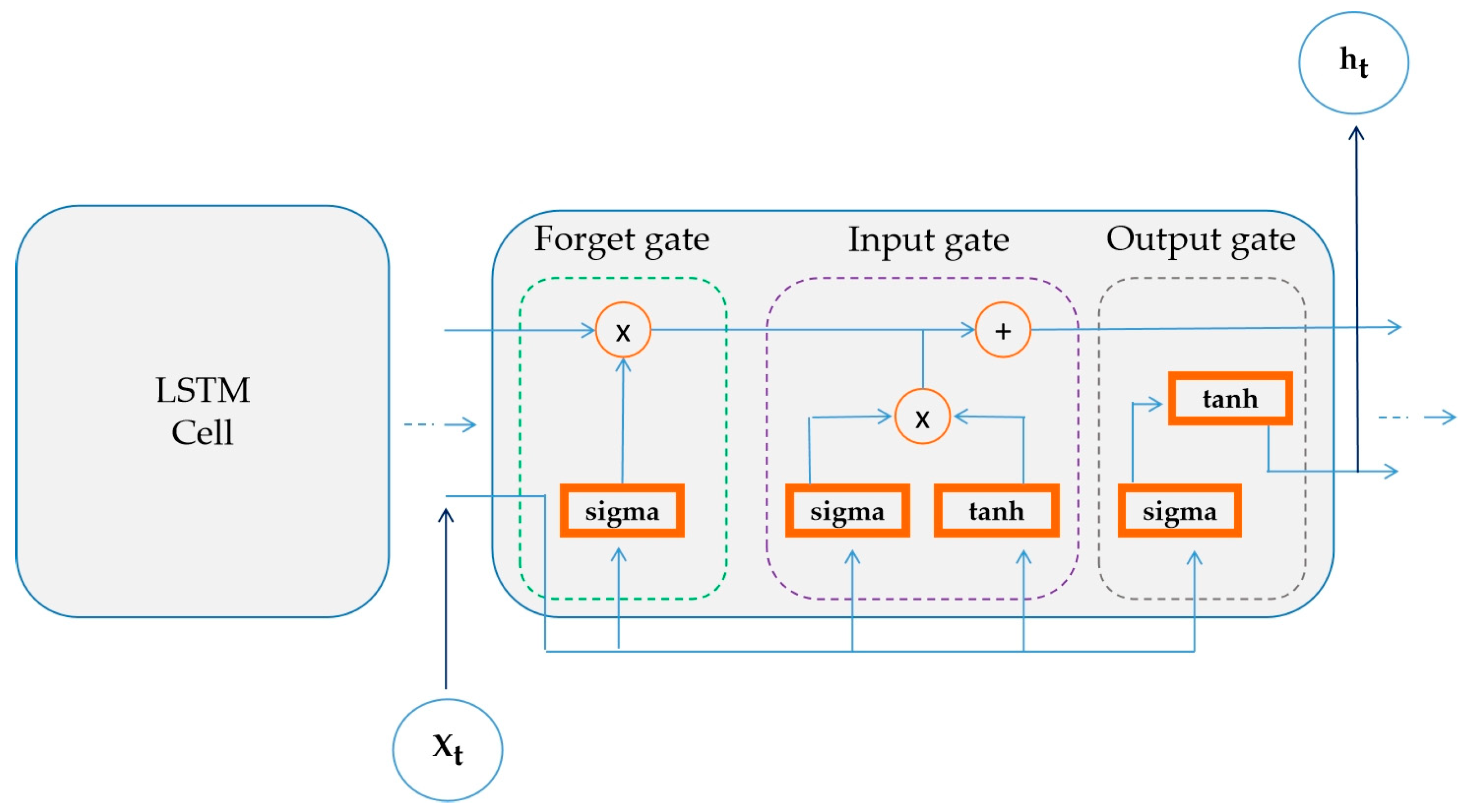
Long Short-Term Memory
Multilayer Perceptron
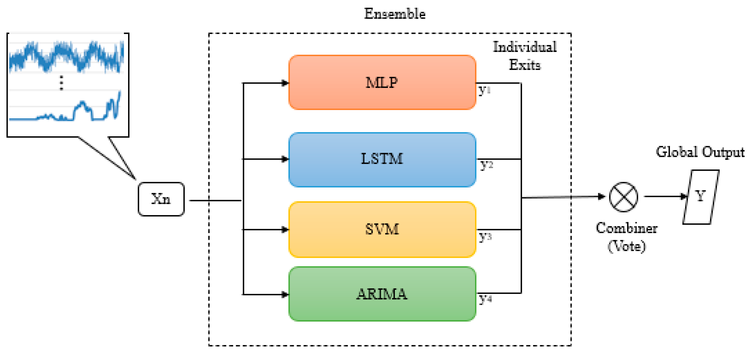
3.2. Ensemble
3.3. General and Relevant Aspects of the Proposed Models
3.3.1. Database
3.3.2. Preprocessing
3.3.3. Techniques and Methods to Optimize Parameters
3.3.4. Assessment Metric
3.3.5. Training Cost
4. Results and Discussion
4.1. Results of the GA + LSTM and GA + MLP Combination
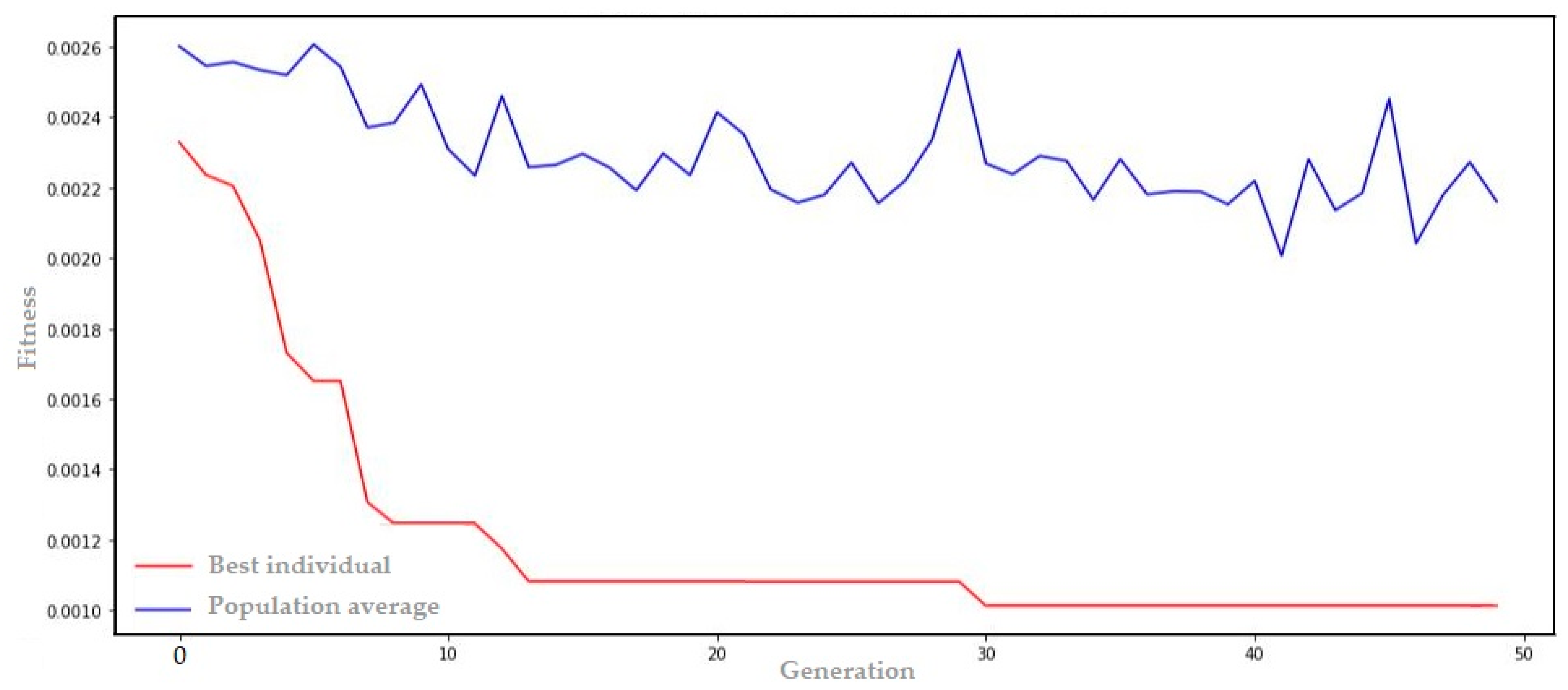
4.1.1. Results of the Combination for PLD
- Genome transcription: [4, 46, 0.01, 57, 0.0, 2, 0.11, 8, 0.03, 0.00101]
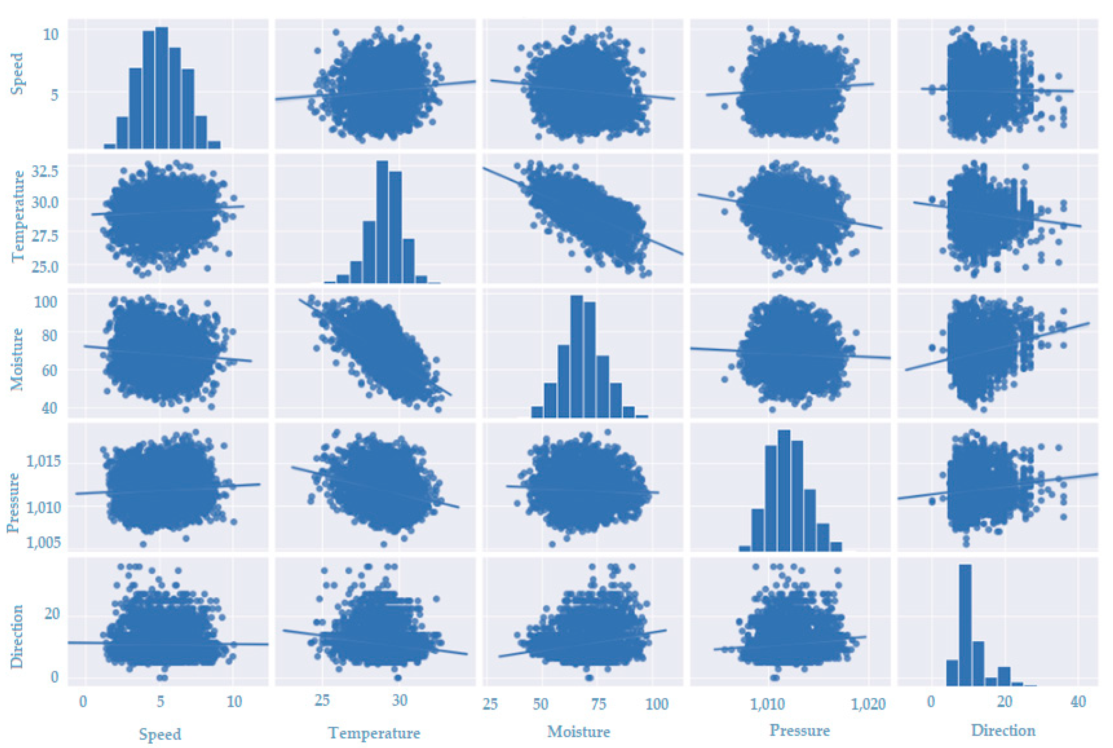
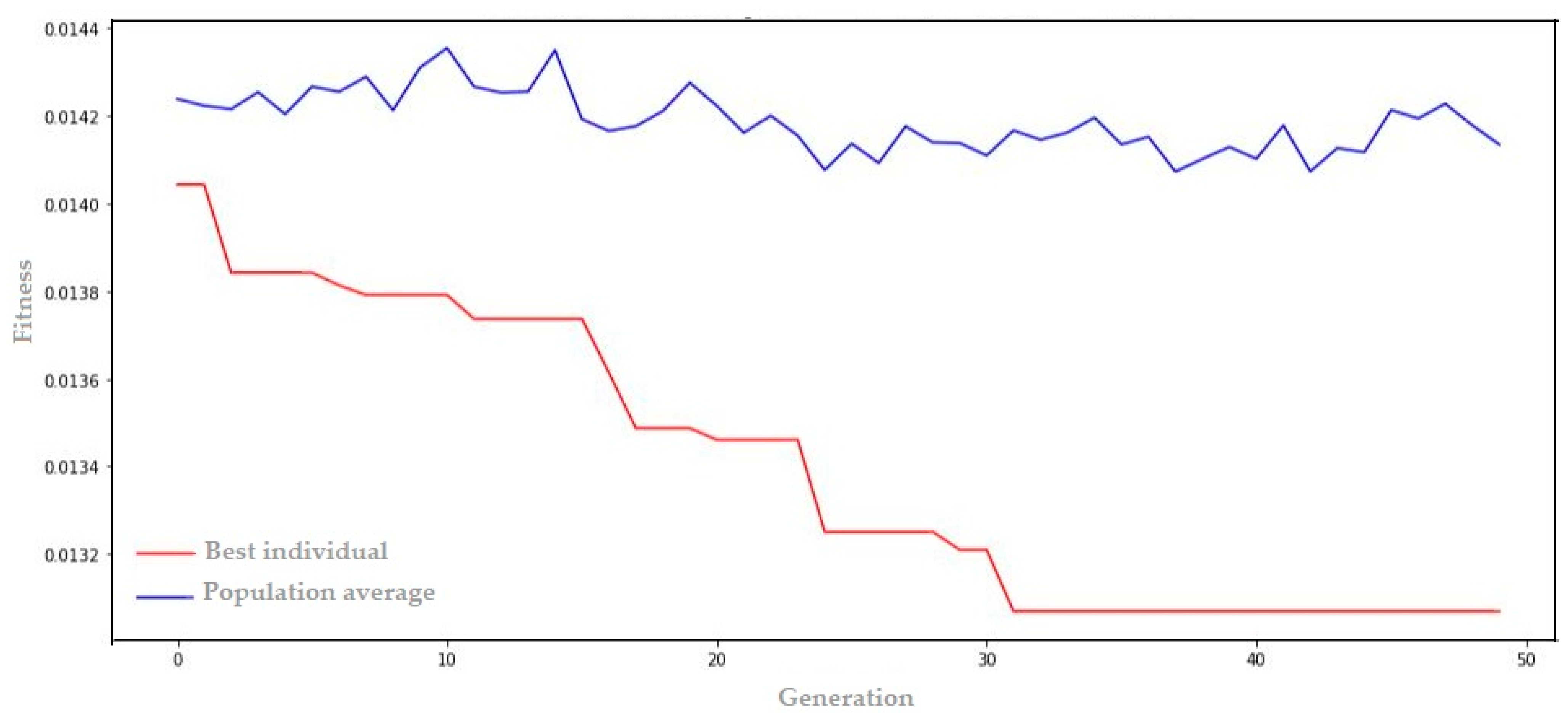
4.1.2. Combination Results for Wind Speed
- Genome transcription: [5, 5, 0.03, 45, 0.09, 36, 0.14, 63, 0.04, 2, 0.02, 0.01306]
4.2. Ensemble Results
4.2.1. Ensemble Results for PLD—North Region
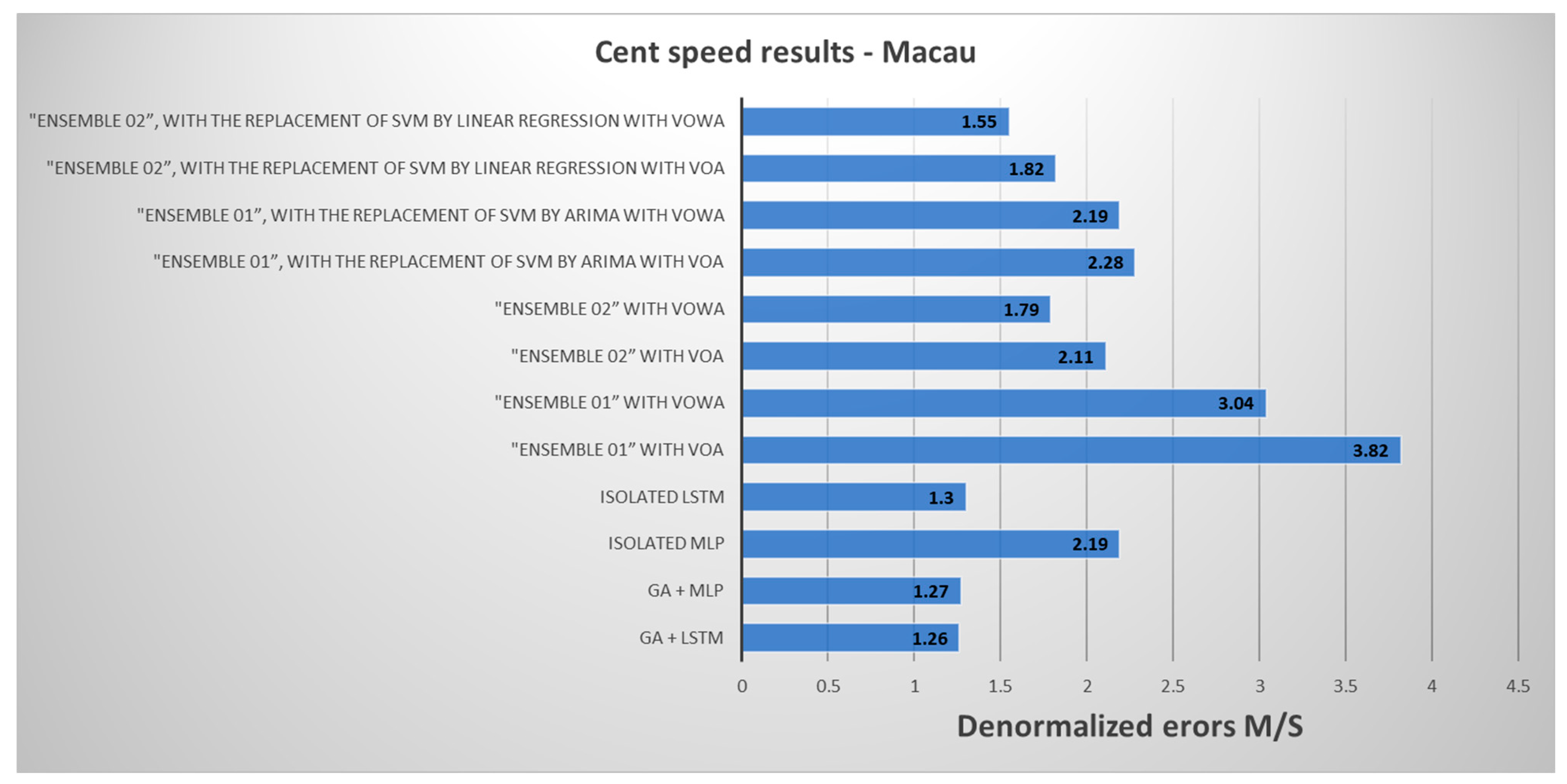
4.2.2. Ensemble Results for Wind Speed—Macau
5. Conclusions
5.1. Practical Implications
5.2. Strengths
5.3. Weaknesses
Author Contributions
Funding
Data Availability Statement
Conflicts of Interest
References
- Electricity Trading Chamber. Available online: https://www.ccee.org.br/ (accessed on 5 June 2023). (In Portuguese).
- Gas Emission Estimation System. Available online: https://seeg.eco.br/ (accessed on 5 June 2023). (In Portuguese).
- Ministry of Science, Technology and Innovation. Available online: https://www.gov.br/mcti/pt-br (accessed on 5 June 2023). (In Portuguese)
- Organization for Economic Co-Operation and Development. Available online: https://www.gov.br/economia/pt-br/assuntos/ocde (accessed on 5 June 2023). (In Portuguese)
- Ministry of Mines and Energy. Available online: https://www.gov.br/mme/ (accessed on 11 April 2023). (In Portuguese)
- Infovento. Available online: https://abeeolica.org.br/dados-abeeolica/infovento-29/ (accessed on 13 January 2023). (In Portuguese).
- National Electric Energy Agency. Available online: https://www.gov.br/aneel/ (accessed on 11 April 2023). (In Portuguese)
- Kotyrba, M.; Volna, E.; Habiballa, H. The Influence of Genetic Algorithms on Learning Possibilities of Artificial Neural Networks. Computers 2022, 11, 70. [Google Scholar] [CrossRef]
- Tran, L.; Le, A.; Nguyen, T.; Nguyen, D.T. Explainable Machine Learning for Financial Distress Prediction: Evidence from Vietnam. Data 2022, 7, 160. [Google Scholar] [CrossRef]
- Ambrioso, J.; Brentan, B.; Herrera, M.; Luvizotto, E., Jr.; Ribeiro, L.; Izquierdo, J. Committee Machines for Hourly Water Demand Forecasting in Water Supply Systems. Math. Probl. Eng. 2019, 2019, 9765468. [Google Scholar] [CrossRef]
- Wang, S.; Roger, M.; Sarrazin, J.; Perrault, C. Hyperparameter Optimization of Two-Hidden-Layer Neural Networks for Power Am-plifiers Behavioral Modeling Using Genetic Algorithms. IEEE Microw. Wirel. Compon. Lett. 2019, 29, 802–805. [Google Scholar] [CrossRef]
- Coordination for the Improvement of Higher Education Personnel. Available online: https://www-periodicos-capes-gov-br.ezl.periodicos.capes.gov.br/index.php?/ (accessed on 3 October 2023). (In Portuguese)
- Bhattacharyya, S. Markets for electricity supply. In Energy Economics, 2nd ed.; Springer: London, UK, 2019; pp. 699–733. [Google Scholar]
- Maciejowska, K. Assessing the impact of renewable energy sources on the electricity price level and variability—A quantile regression approach. Energy Econ. 2020, 85, 104532. [Google Scholar] [CrossRef]
- Junior, F. Direct and Recurrent Neural Networks in Predicting the Price of Short-Term Electricity in the Brazilian Market. Master’s Thesis, Federal University of Pará, Belém, PA, Brazil, 2016. (In Portuguese). [Google Scholar]
- Ribeiro, M.H.D.M.; Stefenon, S.F.; de Lima, J.D.; Nied, A.; Mariani, V.C.; Coelho, L.d.S. Electricity Price Forecasting Based on Self-Adaptive Decomposition and Heterogeneous Ensemble Learning. Energies 2020, 13, 5190. [Google Scholar] [CrossRef]
- Corso, M.P.; Stefenon, S.F.; Couto, V.F.; Cabral, S.H.L.; Nied, A. Evaluation of methods for electric field calculation in transmission lines. IEEE Lat. Am. Trans. 2018, 16, 2970–2976. [Google Scholar] [CrossRef]
- Filho, J.; Affonso, C.; Oliveira, R. Energy price prediction multi-step ahead using hybrid model in the Brazilian market. Electr. Power Syst. Res. 2014, 117, 115–122. [Google Scholar] [CrossRef]
- Hong, T.; Pinson, P.; Wang, Y.; Weron, R.; Yang, D.; Zareipour, H. Energy Forecasting: A Review and Outlook. IEEE Open Access J. Power Energy 2020, 7, 376–388. [Google Scholar] [CrossRef]
- Ozcanli, A.; Yaprakdal, F.; Baysal, M. Deep learning methods and applications for electrical power systems: A comprehensive review. Energy Res. 2020, 44, 7136–7157. [Google Scholar] [CrossRef]
- Abedinia, O.; Lotfi, M.; Bagheri, M.; Sobhani, B.; Shafie-khah, M.; Catalão, J. Improved EMD-Based Complex Prediction Model for Wind Power Forecasting. IEEE Open Access J. Power Energy 2020, 11, 2790–2802. [Google Scholar] [CrossRef]
- Heydari, A.; Nezhad, M.; Pirshayan, E.; Garcia, D.; Keynia, F.; Santoli, L. Short-term electricity price and load forecasting in isolated power grids based on composite neural network and gravitational search optimization algorithm. Appl. Energy 2020, 277, 115–503. [Google Scholar] [CrossRef]
- Chen, W.; Chen, Y.; Tsangaratos, P.; Llia, L.; Wang, X. Combining Evolutionary Algorithms and Machine Learning Models in Landslide Susceptibility Assessments. Remote Sens. 2020, 12, 3854. [Google Scholar] [CrossRef]
- Luo, X.; Oyedele, L.; Ajayi, A.; Akinade, O.; Delgado, J.; Owolabi, H.; Ahmed, A. Genetic algorithm-determined deep feedforward neural network architecture for predicting electricity consumption in real buildings. Energy AI 2020, 2, 100015. [Google Scholar] [CrossRef]
- Alencar, D. Hybrid Model Based on Time Series and Neural Networks for Predicting Wind Energy Generation. Ph.D. Thesis, Federal University of Pará, Belém, PA, Brazil, 2018. (In Portuguese). [Google Scholar]
- Junior, K. Genetic Algorithms and Deep Learning Based on Long Short-Term Memory (LSTM) Recurrent Neural Networks for Medical Diagnosis Assistance. Doctoral Thesis, University of São Paulo, Ribeirão Preto, SP, Brazil, 2023. [Google Scholar] [CrossRef]
- Li, W.; Zang, C.; Liu, D.; Zeng, P. Short-term Load Forecasting of Long-short Term Memory Neural Network Based on Genetic Algorithm. In Proceedings of the 4th IEEE Conference on Energy Internet and Energy System Integration (EI2), Wuhan, China, 30 October–1 November 2020. [Google Scholar] [CrossRef]
- Zulfiqar, M.; Rasheed, M.B. Short-Term Load Forecasting using Long Short Term Memory Optimized by Genetic Algorithm. In Proceedings of the IEEE Sustainable Power and Energy Conference (iSPEC), Perth, Australia, 4–7 December 2022. [Google Scholar] [CrossRef]
- Bendali, W.; Saber, I.; Bourachdi, B.; Boussetta, M.; Mourad, Y. Deep Learning Using Genetic Algorithm Optimization for Short Term Solar Irradiance Forecasting. In Proceedings of the Fourth International Conference on Intelligent Computing in Data Sciences (ICDS), Fez, Morocco, 21–23 October 2020. [Google Scholar] [CrossRef]
- Al Mamun, A.; Hoq, M.; Hossain, E.; Bayindir, R. A Hybrid Deep Learning Model with Evolutionary Algorithm for Short-Term Load Forecasting. In Proceedings of the 8th International Conference on Renewable Energy Research and Applications (ICRERA), Brasov, Romania, 3–6 November 2019. [Google Scholar] [CrossRef]
- Huang, C.; Karimi, H.R.; Mei, P.; Yang, D.; Shi, Q. Evolving long short-term memory neural network for wind speed forecast-ing. Inf. Sci. 2023, 632, 390–410. [Google Scholar] [CrossRef]
- Shahid, F.; Zameer, A.; Muneeb, M. A novel genetic LSTM model for wind power forecast. Energy 2021, 223, 120069. [Google Scholar] [CrossRef]
- ul Islam, B.; Baharudin, Z.; Nallagownden, P.; Raza, M.Q. A Hybrid Neuro-Genetic Approach for STLF: A Comparative Analy-sis of Model Parameter Variations. In Proceedings of the IEEE 8th International Power Engineering and Optimization Conference (PEOCO2014), Langkawi, Malaysia, 24–25 March 2014. [Google Scholar] [CrossRef]
- Izidio, D.M.F.; de Mattos Neto, P.S.G.; Barbosa, L.; de Oliveira, J.F.L.; Marinho, M.H.d.N.; Rissi, G.F. Evolutionary Hybrid Sys-tem for Energy Consumption Forecasting for Smart Meters. Energies 2021, 14, 1794. [Google Scholar] [CrossRef]
- Elsken, T.; Metzen, J.; Hutter, F. Neural Architecture Search. Autom. Mach. Learn. 2019, 63–77. [Google Scholar] [CrossRef]
- Wang, S.; Zhang, N.; Wu, L.; Wang, Y. Wind speed forecasting based on the hybrid ensemble empirical mode decomposition and GA-BP neural network method. Renew. Energy 2016, 94, 629e636. [Google Scholar] [CrossRef]
- Cao, Y.; Liu, G.; Luo, D.; Bavirisetti, D.P.; Xiao, G. Multi-timescale photovoltaic power forecasting using an improved Stacking ensemble algorithm based LSTM-Informer model. Energy 2023, 283, 128669. [Google Scholar] [CrossRef]
- Shi, J.; Teh, J. Load forecasting for regional integrated energy system based on complementary ensemble empirical mode de-composition and multi-model fusion. Appl. Energy 2024, 353, 122146. [Google Scholar] [CrossRef]
- Wu, Z.; Wang, B. An Ensemble Neural Network Based on Variational Mode Decomposition and an Improved Sparrow Search Algorithm for Wind and Solar Power Forecasting. IEEE Access 2021, 9, 166709. [Google Scholar] [CrossRef]
- Ribeiro, M.; da Silva, G.; Canton, C.; Fraccanabbi, N.; Mariani, C.; Coelho, S. Electricity energy price forecasting based on hybrid multi-stage heterogeneous ensemble: Brazilian commercial and residential cases. In Proceedings of the International Joint Conference on Neural Networks (IJCNN), Glasgow, UK, 19–24 July 2020. [Google Scholar] [CrossRef]
- Doan, Q.; Le, T.; Thai, D. Optimization strategies of neural networks for impact damage classification of RC panels in a small dataset. Appl. Soft Comput. 2021, 102, 107100. [Google Scholar] [CrossRef]
- Kadhim, Z.; Abdullah, H.; Ghathwan, K. Artificial Neural Network Hyperparameters Optimization: A Survey. Int. J. Online Biomed. Eng. 2022, 18, 15. [Google Scholar] [CrossRef]
- Masís, A.; Cruz, A.; Schierholz, M.; Duan, X.; Roy, K.; Yang, C.; Donadio, R.; Schuster, C. ANN Hyperparameter Optimization by Genetic Algorithms for Via Interconnect Classification. In Proceedings of the IEEE 25th Workshop on Signal and Power Integrity (SPI), Siegen, Germany, 10–12 May 2021. [Google Scholar]
- Phyo, P.; Byun, Y. Hybrid Ensemble Deep Learning-Based Approach for Time Series Energy Prediction. Symmetry 2021, 13, 1942. [Google Scholar] [CrossRef]
- Yang, X. Nature-Inspired Optimization Algorithms, 2nd ed.; Academic Press: London, UK, 2020; pp. 107–118. [Google Scholar]
- Kochenderfer, M.; Wheeler, T. Algorithms for Optimization, 1st ed.; Mit Press: London, UK, 2019; pp. 147–162. [Google Scholar]
- Garbin, C.; Zhu, X.; Marques, O. Dropout vs. batch normalization: An empirical study of their impact to deep learning. Multimed. Tools Appl. 2020, 79, 12777–12815. [Google Scholar] [CrossRef]
- Akhtar, S.; Shahzad, S.; Zaheer, A.; Ullah, H.; Kilic, H.; Gono, R.; Jasinski, M.; Leonowicz, Z. Short-Term Load Forecasting Models: A Review of Challenges, Progress, and the Road Ahead. Energies 2023, 16, 4060. [Google Scholar] [CrossRef]
- Kurani, A.; Doshi, P.; Vakharia, A.; Shah, M. A Comprehensive Comparative Study of Artificial Neural Network (ANN) andSupport Vector Machines (SVM) on Stock Forecasting. Ann. Data Sci. 2023, 10, 183–208. [Google Scholar] [CrossRef]
- Dagoumas, A.; Koltsaklis, N. Review of models for integrating renewable energy in the generation expansion planning. Appl. Energy 2019, 242, 1573–1587. [Google Scholar] [CrossRef]
- Hur, Y. An Ensemble Forecasting Model of Wind Power Outputs based on Improved Statistical Approaches. Energies 2020, 13, 1071. [Google Scholar] [CrossRef]
- Carneiro, T.; Rocha, P.; Carvalho, P.; Ramírez, L. Ridge regression ensemble of machine learning models applied to solar and wind forecasting in Brazil and Spain. Appl. Energy 2022, 314, 118936. [Google Scholar] [CrossRef]
- Sagi, O.; Rokach, L. Ensemble learning: A survey. WIREs Data Mining Knowl Discov. 2018, 8, e1249. [Google Scholar] [CrossRef]
- Solano, E.S.; Affonso, C.M. Solar Irradiation Forecasting Using Ensemble Voting Based on Machine Learning Algorithms. Sustainability 2023, 15, 7943. [Google Scholar] [CrossRef]
- Phyo, P.-P.; Byun, Y.-C.; Park, N. Short-Term Energy Forecasting Using Machine-Learning-Based Ensemble Voting Regression. Symmetry 2022, 14, 160. [Google Scholar] [CrossRef]
- Alymani, M.; Mengash, H.A.; Aljebreen, M.; Alasmari, N.; Allafi, R.; Alshahrani, H.; Elfaki, M.A.; Hamza, M.A.; Abdelmageed, A.A. Sustainable residential building energy consumption forecasting for smart cities using optimal weighted voting ensemble learning. Sustain. Energy Technol. Assess. 2023, 57, 103271. [Google Scholar] [CrossRef]
- Christoph, E.; Raviv, E.; Roetzer, G. Forecast Combinations in R using the ForecastComb Package. R J. 2019, 10, 262. [Google Scholar] [CrossRef]
- Villanueva, W. Committee on Machines in Time Series Prediction. Master’s Thesis, Campinas State University, Campinas, SP, Brazil, 2006. (In Portuguese). [Google Scholar]
- Zhou, Q.; Wang, C.; Zhang, G. A combined forecasting system based on modified multi-objective optimization and sub-model selection strategy for short-term wind speed. Appl. Soft Comput. 2020, 94, 106463. [Google Scholar] [CrossRef]
- Lv, S.; Wang, L.; Wang, S. A Hybrid Neural Network Model for Short-Term Wind Speed Forecasting. Energies 2023, 16, 1841. [Google Scholar] [CrossRef]
- Wang, L. Advanced Multivariate Time Series Forecasting Models. J. Math. Stat. 2018, 14, 253–260. [Google Scholar] [CrossRef]
- Conte, T.; Santos, W.; Nunes, L.; Veras, J.; Silva, J.; Oliveira, R. Use of ARIMA and SVM for forecasting time series of the Brazilian electrical system. Res. Soc. Dev. 2023, 12, 3. [Google Scholar] [CrossRef]
- Bitirgen, K.; Filik, U. Electricity Price Forecasting based on XGBooST and ARIMA Algorithms. J. Eng. Res. Technol. 2020, 1, 7–13. [Google Scholar]
- National Environmental Data Organization System (SONDA). Available online: http://sonda.ccst.inpe.br/basedados/ (accessed on 11 April 2023). (In Portuguese).
- Puheim, M.; Madarász, L. Normalization of inputs and outputs of neural network based robotic arm controller in role of inverse kinematic model. In Proceedings of the IEEE 12th International Symposium on Applied Machine Intelligence and Informatics (SAMI), Herl’any, Slovakia, 23–25 January 2014. [Google Scholar] [CrossRef]
- Lee, S.; Kim, J.; Kang, H.; Kang, D. Genetic Algorithm Based Deep Learning Neural Network Structure and Hyperparameter Optimization. Appl. Sci. 2021, 11, 774. [Google Scholar] [CrossRef]
- Géron, A. Hands-on Machine Learning with Scikit-Learn, Keras, and TensorFlow: Concepts, Tools, and Techniques to Build Intelligent Systems, 2nd ed.; O’Reilly Media: Sebastopol, CA, USA, 2020; pp. 62–70. [Google Scholar]
- Carvalho, A.; Gama, J.; Lorena, A.; Faceli, K. Artificial Intelligence: A Machine Learning Approach, 1st ed.; LTC: Rio de Janeiro, Brazil, 2011; p. 394. (In Portuguese) [Google Scholar]
- Bradshaw, A. Electricity Market Reforms and Renewable Energy: The Case of Wind and Solar in Brazil. Ph.D. Thesis, Columbia University, New York, NY, USA, 2018. [Google Scholar]
- Camelo, H.; Lucio, P.; Junior, J.; Carvalho, P. Time Series Forecasting Methods and Hybrid Modeling both Applied to Monthly Average Wind Speed for Northeastern Regions of Brazil. Braz. Meteorol. Mag. 2017, 32, 565–574. (In Portuguese) [Google Scholar] [CrossRef]
- Belentani, Y. Short-Term Market Energy Price Forecasting: A Combined Analysis of Time Series and Artificial Neural Networks. Master’s Thesis, São Paulo University, São Paulo, Brazil, 2023. (In Portuguese). [Google Scholar]
- Santos, C.; Silva, L.; Castro, R.; Marques, R. Application of machine learning to project the hourly price for settlement of differences to support electricity trading strategies. Braz. Energy Mag. 2022, 28, 243–279. [Google Scholar] [CrossRef]


| Bibliographic Research | Number of Articles |
|---|---|
| Machine learning time series | 68,557 |
| Machine learning to predict the price of Brazilian electricity | 136 |
| Recurrent neural networks for forecasting Brazilian electricity | 72 |
| Deep neural networks for forecasting the price of electricity in Brazil | 113 |
| Long short-term memory Brazilian electricity system | 78 |
| Incorporating a combination of long short-term memory (LSTM) and genetic algorithm techniques for optimizing the Brazilian electricity system. | 79 |
| Hybrid model for the Brazilian electrical system | 3316 |
| Hybrid models to predict the price of Brazilian electricity | 208 |
| Assemble to predict for the Brazilian electrical system | 467 |
| Assemble to predict the price of Brazilian electricity | - |
| Parameters | Values/Description |
|---|---|
| Population | 80 individuals |
| Elitism | The n best individuals from the previous population are chosen (n = 1) |
| Crossover probability | 75% (with two cut-off points) |
| Mutation | Individuals’ genes can change with a probability of 1% |
| Selection | Random selection by tournament |
| Ensemble 01 Members | Parameters |
| Decision tree | Measurement at each tree node: mean squared error (MSE); Node splitting: “best” (best possible split); Tree depth: 5. |
| Linear regression | Method fit; fit_intercept: True; copy_X: True; n_jobs: None; positive bool: False. |
| SVM | Method random search (PLD Dataset): C: 70.645; Gamma: 4.64 × 10⁻⁶; Epsilon: 0.230; Method Bayes search (Macau Dataset): C: 5.202; Gamma: auto Epsilon: 0.061. |
| MLP | 2 hidden layers with 64 neurons each; Non-linear activation function in all hidden layers: “relu”; Epochs for training: 50; Activation function in the output layer: Linear; Weight update: ‘adam’. |
| Ensemble 02 Members | Parameters |
| MLP e LSTM | Epochs for training: 100; Non-linear activation function in all hidden layers: “relu”; Activation function in the output layer: Linear; Weight update: ‘RMSProp’ optimizer. |
| SVM | Method random search (PLD Dataset): C: 70.645; Gamma: 4.64 × 10⁻⁶; Epsilon: 0.230; Method Bayes search (Macau Dataset): C: 5.202; Gamma: auto Epsilon: 0.061. |
| ARIMA | Dickey–Fuller stationarity test; Grid-Search technique; The traditional statistical method proposed by George Box and Gwilym Jenkins, which involves the use of AutoRegressive Integrated Moving Average models (ARIMA(p, d, q)). |
| Measurements | PLD | Hydraulics | Thermal | Charge | EARM | ENA |
|---|---|---|---|---|---|---|
| average | 66.66 | 3636.02 | 0.00 | 3091.66 | 106.44 | 93.00 |
| Minimun | 4.00 | 539.00 | 0.00 | 376.43 | 8.73 | 31.86 |
| Maximun | 684.00 | 14,795.00 | 0.00 | 6922.29 | 13,948.34 | 264.43 |
| Amplitude | 680.00 | 14,256.00 | 0.00 | 6545.86 | 13,939.61 | 232.57 |
| Variance | 13,353 | 18,106.00 | 0 | 345,297.7519 | 446,677.2 | 1130.133 |
| Standard deviation | 115.68 | 1347.11 | 0 | 588.2847683 | 669.0948 | 33.65546 |
| Median | 18.59 | 3382.14 | 0.00 | 3165.43 | 67.20 | 87.29 |
| Mode | 18.59 | 3876 | 0 | 2622.14 | 73.81 | 97 |
| Measurements | Speed | Temperature | Moisture | Pressure | Direction |
|---|---|---|---|---|---|
| average | 5.17 | 29.04 | 68.42 | 1011.94 | 11.07 |
| Minimun | 1.15 | 24.20 | 39.00 | 1005.63 | 0.00 |
| Maximun | 10.07 | 32.70 | 98.00 | 1018.73 | 36.00 |
| Amplitude | 8.92 | 8.50 | 59.00 | 13.10 | 36.00 |
| Variance | 2.25051 | 1.21818 | 85.6184 | 3.7769 | 19.6294 |
| Standard deviation | 1.50032 | 1.10383 | 9.25397 | 1.94362 | 4.43096 |
| Median | 5.10 | 29.13 | 68.00 | 1011.87 | 9.33 |
| Mode | 5.3 | 29 | 71 | 1012.3 | 9.33 |
| Hyperparameter Optimization | ARIMA | SVM | LSTM | MLP | Decision Tree | Linear Regression | Characteristics |
|---|---|---|---|---|---|---|---|
| Auto ARIMA | ✓ | x | x | x | x | x | Determines the values of P, D, and Q; uses the Akaike information criterion (AIC) to choose the best model. |
| Grid Search | ✓ | x | x | x | x | x | Greater focus on errors; test in all possible combinations; identifies the ideal model based on errors. |
| Random Search | x | ✓ | x | x | x | x | C, Epsilon and Gamma optimization; test in different combinations, but randomly; the goal is to minimize execution time. |
| Baves Search | x | ✓ | x | x | x | x | Optimize C, Epsilon and Gamma; speeds up the search, as it reuses information at points from past interactions; |
| Method fit | x | x | x | x | x | ✓ | Finding the best parameters that minimize the error between the model predictions and the actual values in the training set. |
| Genetic Algorithm | x | x | ✓ | ✓ | x | x | Canonical with the characteristics of elitism and selection by tournament. |
| Manually tuned | x | x | ✓ | ✓ | ✓ | x | Number of layers, number of neurons/cells, update of weights; training times, hidden and output layer activation function, evaluation metrics, tree depth and node division. |
| GA + Deep Learning | North |
|---|---|
| GA + LSTM | 0.00101 |
| GA + MLP | 0.00183 |
| GA + Deep Learning | Macau |
|---|---|
| GA + LSTM | 0.01306 |
| GA + MLP | 0.01429 |
| MLP | Decision Tree | Linear Regression | SVM | |
| “ensemble 01” | 4 | 3 | 2 | 1 |
| MLP | LSTM | SVM | ARIMA | |
| “ensemble 02” | 4 | 3 | 2 | 1 |
| Evaluation Metric | Decision Tree | MLP | SVM | Linear Regression | “Ensemble 01” with VOA | “Ensemble 01” with VOWA |
|---|---|---|---|---|---|---|
| MSE | 0.00220 | 0.002941 | 0.74488 | 0.002353 | 0.18823 | 0.15082 |
| Evaluation Metric | MLP | LSTM | SVM | ARIMA (16, 0, 24) | “Ensemble 02” with VOA | “Ensemble 02” with VOWA |
|---|---|---|---|---|---|---|
| MSE | 0.00233 | 0.00252 | 0.78235 | 0.09720 | 0.22115 | 0.16823 |
| Evaluation Metric | “Ensemble 01” with VOA | “Ensemble 01” with VOWA |
|---|---|---|
| MSE | 0.02617 | 0.01308 |
| Evaluation Metric | “Ensemble 02” with VOA | “Ensemble 02” with VOWA |
|---|---|---|
| MSE | 0.02610 | 0.01185 |
| Evaluation Metric | Decision Tree | MLP | SVM | Linear Regression | “Ensemble 01” with VOA | “Ensemble 01” with VOWA |
|---|---|---|---|---|---|---|
| MSE | 0.11348 | 0.11731 | 0.85393 | 0.11235 | 0.30056 | 0.18988 |
| Evaluation Metric | MLP | LSTM | SVM | ARIMA (23, 0, 25) | “Ensemble 02” with VOA | “Ensemble 02” with VOWA |
|---|---|---|---|---|---|---|
| MSE | 0.01348 | 0.01685 | 0.22247 | 0.16629 | 0.10561 | 0.07191 |
| Evaluation Metric | “Ensemble 01” with VOA | “Ensemble 01” with VOWA |
|---|---|---|
| MSE | 0.12696 | 0.11797 |
| Evaluation Metric | “Ensemble 02” with VOA | “Ensemble 02” with VOWA |
|---|---|---|
| MSE | 0.07640 | 0.04494 |
Disclaimer/Publisher’s Note: The statements, opinions and data contained in all publications are solely those of the individual author(s) and contributor(s) and not of MDPI and/or the editor(s). MDPI and/or the editor(s) disclaim responsibility for any injury to people or property resulting from any ideas, methods, instructions or products referred to in the content. |
© 2024 by the authors. Licensee MDPI, Basel, Switzerland. This article is an open access article distributed under the terms and conditions of the Creative Commons Attribution (CC BY) license (https://creativecommons.org/licenses/by/4.0/).
Share and Cite
Conte, T.; Oliveira, R. Comparative Analysis between Intelligent Machine Committees and Hybrid Deep Learning with Genetic Algorithms in Energy Sector Forecasting: A Case Study on Electricity Price and Wind Speed in the Brazilian Market. Energies 2024, 17, 829. https://doi.org/10.3390/en17040829
Conte T, Oliveira R. Comparative Analysis between Intelligent Machine Committees and Hybrid Deep Learning with Genetic Algorithms in Energy Sector Forecasting: A Case Study on Electricity Price and Wind Speed in the Brazilian Market. Energies. 2024; 17(4):829. https://doi.org/10.3390/en17040829
Chicago/Turabian StyleConte, Thiago, and Roberto Oliveira. 2024. "Comparative Analysis between Intelligent Machine Committees and Hybrid Deep Learning with Genetic Algorithms in Energy Sector Forecasting: A Case Study on Electricity Price and Wind Speed in the Brazilian Market" Energies 17, no. 4: 829. https://doi.org/10.3390/en17040829