A Control-Oriented Model for Predicting Variations in Membrane Water Content of an Open-Cathode Proton Exchange Membrane Fuel Cell

Abstract

Proton exchange membrane (PEM) fuel cells have emerged as a viable alternative energy production source for stationary and transportation applications. Reliable and sustainable fuel cell operation requires effective water management. Membrane water content can vary along the stack during transients which can lead to losses in fuel cell performance. To control these variations, a model that predicts the internal humidity dynamics of the stack is needed. In this study, a control-oriented model for predicting membrane water content variation was developed and implemented in MATLAB/Simulink. A lumped parameter model was initially developed and then further discretized into smaller control volumes to track humidity distribution along the stack. To validate the model’s predictions, the predicted results were compared to computer simulation results from GT-Suite. The root mean square error (RMSE) between the model’s prediction and GT-Suite’s simulation results was found to be within 1.5 membrane water content for all cases, demonstrating the model’s capability to capture the variation in membrane water content along the stack. The developed model will be useful for real-time control of membrane water content distribution in PEM fuel cells.

1. Introduction

Due to the negative environmental impacts of fossil fuels, alternatives are being sought and developed, particularly in the transportation sector where reliance on petroleum-based fuels is high. While the electrification of light-duty vehicles is growing, medium and heavy-duty vehicles can be harder to electrify due to their high energy demands. For medium to heavy-duty vehicles, proton exchange membrane (PEM) fuel cells have received considerable attention. Fuel cells provide an electrification solution for vehicles that alleviates range anxiety due to their refueling capability. They can also function with better efficiency than internal combustion engines and produce little to no pollutants on board. Among various fuel cell types, the PEM fuel cell stands out as a popular choice, primarily due to its high power density and low operating temperature.

There are two types of PEM fuel cells: the closed-cathode and open-cathode varieties. The closed-cathode design is usually equipped with a compressor, a manifold, a dedicated cooling circuit for temperature management, and an external humidifier for water management. These auxiliary components in the closed-cathode design induce parasitic loads that impact the stack performance. In contrast, the open-cathode design reduces the system’s complexity by integrating the stack’s air supply and temperature control and consequently water management.

Typically, the polymer electrolyte membrane in PEM fuel cells is responsible for the proton conductivity that allows the movement of protons from the anode to the cathode, making it a crucial component of the stack. Due to their excellent chemical and mechanical qualities as well as their high proton conductivity, membranes based on perfluorosulfonic acid polymers such as Nafion, developed by Dupont in the late 1960s, are widely employed in a variety of fuel cell types [1]. One of the main drawbacks of the Nafion membrane for PEM fuel cell operation is the strong decrease in proton conductivity at low hydration levels. Reliable PEM fuel cell operation, therefore, requires the PEM fuel cell membrane to be well hydrated. Too much water, on the other hand, can block the flow channels, preventing reactants from reaching the reaction sites. As a result, effective water management is critical for the sustained operation of PEM fuel cells.

Membrane humidity has been shown to influence the cell performance. Zeng et al. [2] investigated the performance of an open-cathode PEM fuel cell under variable speed control. They established that a strong air flow rate leads to a decrease in cell voltage due to excessive loss in membrane water content. Further, Morner and Klein [3] evaluated the dynamic behavior of an air-breathing fuel cell stack experimentally and concluded that the performance of the stack is more dependent on membrane humidity than the stack temperature. The effect of cathode relative humidity on the performance and uniformity of PEM fuel cells was investigated by Jeon et al. [4] using numerical studies. High cathode relative humidity was found to improve cell performance. Furthermore, they observed uniform temperature and current density distributions when the membrane was hydrated. Chen et al. [5] showed via a numerical model established in MATLAB that increasing the hydrogen humidity improves the performance of the fuel cell. To study the effects of operation temperature and reactant gas humidity levels on the performance of PEM fuel cells, Ozen et al. [6] utilized single-cell PEM fuel cells with an active area of 25 cm² to observe the desired temperature and humidity conditions. The results indicate that humidification of the inlet gases improves the cell performance, with higher performance observed when the cathode gas was humidified.

The membrane water content needs to be in the right range to promote ionic conductivity but must not interfere with reactant transport. Due to its dependence on temperature and reactant inlet humidity, controlling membrane water content is inherently challenging. Internal cell variations that occur during transients can also lead to losses in fuel cell performance. The spatial inhomogeneity of membrane water content has been experimentally investigated using techniques such as membrane resistance distribution, proton nuclear imaging, neutron imaging, and X-ray radiography to visualize the water distribution. For instance, Watanabe et al. [7] undertook membrane resistance measurements using three platinum probes embedded at different depths of a recast Nafion film. The potential difference between the adjacent platinum wires resulted in membrane internal resistance distribution, with the resistance measurements reflecting the water gradients. Zhang et al. [8] developed a nuclear magnetic resonance (NMR) sequence coding along the depth direction of a membrane, averaging the signal over the sample’s cross-section to visualize the water concentration profile of the membrane. The observed distribution of membrane water content impacts the performance and longevity of the fuel cell stack. To guarantee the stack’s performance and continued operation, these variations must be carefully monitored and controlled. As the fuel cell’s internal humidity status cannot be measured, control strategies depend on models to predict the internal humidity dynamics.

There are a number of existing models that aim to predict humidity distribution in a fuel cell stack. For instance, Zhang and Jiao [9] developed a three-dimensional (3D) mathematical model of a PEM fuel cell. The established model can describe the relative humidity distribution of the gases in the anode and cathode channels as well as the membrane water content. Dutta et al. [10] established a 3D model using Navier Stoke’s equations with a multi-species mixture. They found that species mass flow direction significantly depends on mass consumption on the membrane electrode assembly. To study the water and thermal behavior of an open-cathode PEM fuel cell, Sagar et al. [11] developed a 3D CFD model to predict the spatial distribution of relative humidity, temperature, and membrane water content. They concluded that high water content variations in the fuel cell limit the cell performance. These studies provide insight into the fact there are distributions in the fuel cell stack that impact performance and hence need to be controlled. However, these computationally fluid dynamic (CFD)-based models are not suitable for control purposes as they are far too computationally expensive.

A number of control-oriented models have been created over the years. For instance, Pukrushpan et al. [12] developed a control-oriented lumped-parameter model for automotive fuel cell systems. The model was proven to be useful for the analysis of the transient effect of step inputs and system observability. Meyer and Yao [13] developed a control-oriented model for a self-humidifying fuel cell stack and the model was capable of characterizing the transient response of the fuel cell stack. Chen et al. [14] developed a physics-based model to control the temperature and humidity of a PEM fuel cell power system using multi-input and multi-output fuzzy methods. To study and control the cathode humidity of a PEM fuel cell, Chen et al. [15] developed a dynamic water management model and applied an active disturbance control strategy. Chen et al. [16] developed a lumped parameter control-oriented model for predicting humidity dynamics for an open-cathode PEM fuel cell. Based on their model, the output performance of an open-cathode PEM fuel cell, taking into account the internal humidity state of the stack, is predicted. All these models adopt the lumped-parameter approach, which assumes minimal spatial variations. However, the CFD models reviewed, together with the experimental visualization of membrane water content, demonstrate that variations exist; therefore, control-oriented models must account for these variations to ensure effective control of the membrane water content in the PEM fuel cell stack.

For predicting humidity spatial variations, Headley et al. [17] developed and experimentally validated a control-oriented model that captures the variation in relative humidity along the cathode channel but did not explore humidity variation in the anode channel, which can occur due to back diffusion. It is not possible to accurately capture variations in membrane water content with this approach as the membrane water content depends on humidity dynamics in both the cathode and anode channels. In fact, a more conservative approach to determining the membrane water content is to model it as a function of water activity in the anode alone. Nguyen and White [18] adopted this approach in their work where the membrane water content was taken to be the anode water content to reflect the importance of the anode side water activity as it is often the limiting electrode due to drying conditions. Therefore, for more accurate predictions of variations in membrane water content, a model that predicts variations in humidity along the cathode and anode channels is needed.

The main contribution of this paper is that it overcomes the limitation of existing control-oriented models for water management by developing a model that predicts humidity variations along both the cathode and anode channels, with the goal of providing more accurate insights into the humidity dynamics in the PEM fuel cell membrane. In this study, a reduced-order model that integrates thermal effects to predict spatial variations in membrane water content of a 5 kW open-cathode PEM fuel cell stack is presented. First, a lumped parameter model of the stack was developed. This model was then further discretized into smaller control volumes. The model was validated by comparing its predictions to simulation results from GT-Suite and achieved good agreement. The developed model will be useful for real-time control of membrane water content variation in PEM fuel cells.

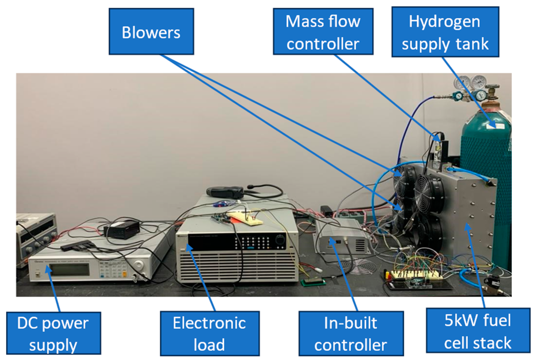
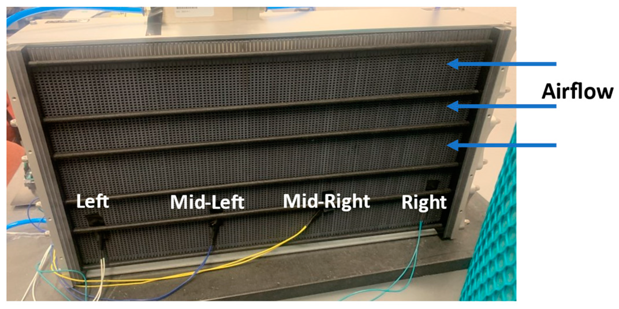
2. Experimental Setup

The model is based on the experimental setup shown in Figure 1. The fuel cell stack is a commercially available 5 kW open-cathode stack from Horizon. It has 120 cells connected in series. The active area of each cell is 150 cm². Air is supplied to the stack by four blowers connected to the casing of the stack. Hydrogen of 99.99% purity is supplied to the stack from a pressurized tank. The stack is equipped with an in-built controller from the manufacturer that monitors and records the current, voltage, and stack temperature. A mass flow controller from Aalborg is used to measure the hydrogen inlet pressure and control the supply of hydrogen to the anode. There are also four thermocouples which are attached on the other side of the stack casing (opposite the fans) with the aim of monitoring temperature variation along the stack (Figure 2). Data taken on this experimental setup was used for model validation.

Experimental Procedure

For data collection, the PEM fuel cell stack was initially warmed up for a 30 min period to humidify the stack. The load was varied from 0 A to 85 A for the test. After the warm-up, and with the load set to a current of 0 A, the hydrogen gas mass flow rate, gas temperature, and pressure data were logged by the Aalborg mass flow controller. The in-stack temperature, current, and voltage were concurrently logged by the in-built controller from Horizon. At the same time, the thermocouple data were acquired via a MATLAB code. Counting from the direction of airflow as shown in Figure 2, the temperature for the right thermocouple was taken from membrane electrode assembly (MEA) #8, the mid-right thermocouple from MEA #43, the mid-left thermocouple from MEA #82, and the left thermocouple from MEA #113. For each load, data were logged for approximately 5 min before proceeding to the next load. Data from the last minute for each load were averaged to obtain the steady state values. The minimum and maximum steady state values recorded for the test are summarized in

Table 1. Minimum and maximum steady state values for test parameters.

Test Parameters	Minimum	Maximum
Gas mass flow rate (kg/s)	$4.1067\times {10}^{-6}$	0.000111
Gas pressure (Pa)	129,863	163,974
Gas temperature (K)	303.49	305
Right thermocouple (K)	296.42	307.21
Mid-right thermocouple (K)	297.04	312.70
Mid-left thermocouple (K)	296.51	305.85
Left thermocouple (K)	297.02	315.32
In-Stack Temperature (K)	295.15	327.15
Voltage (V)	67.10	116.60

. The test was carried out at a constant 90 PWM fan speed to study the variations in membrane water content at this set fan speed. The acquired gas mass flow rate, gas temperature, and pressure as well as the current load served as input to the models. The stack voltage data and recorded temperatures were utilized for model validation.

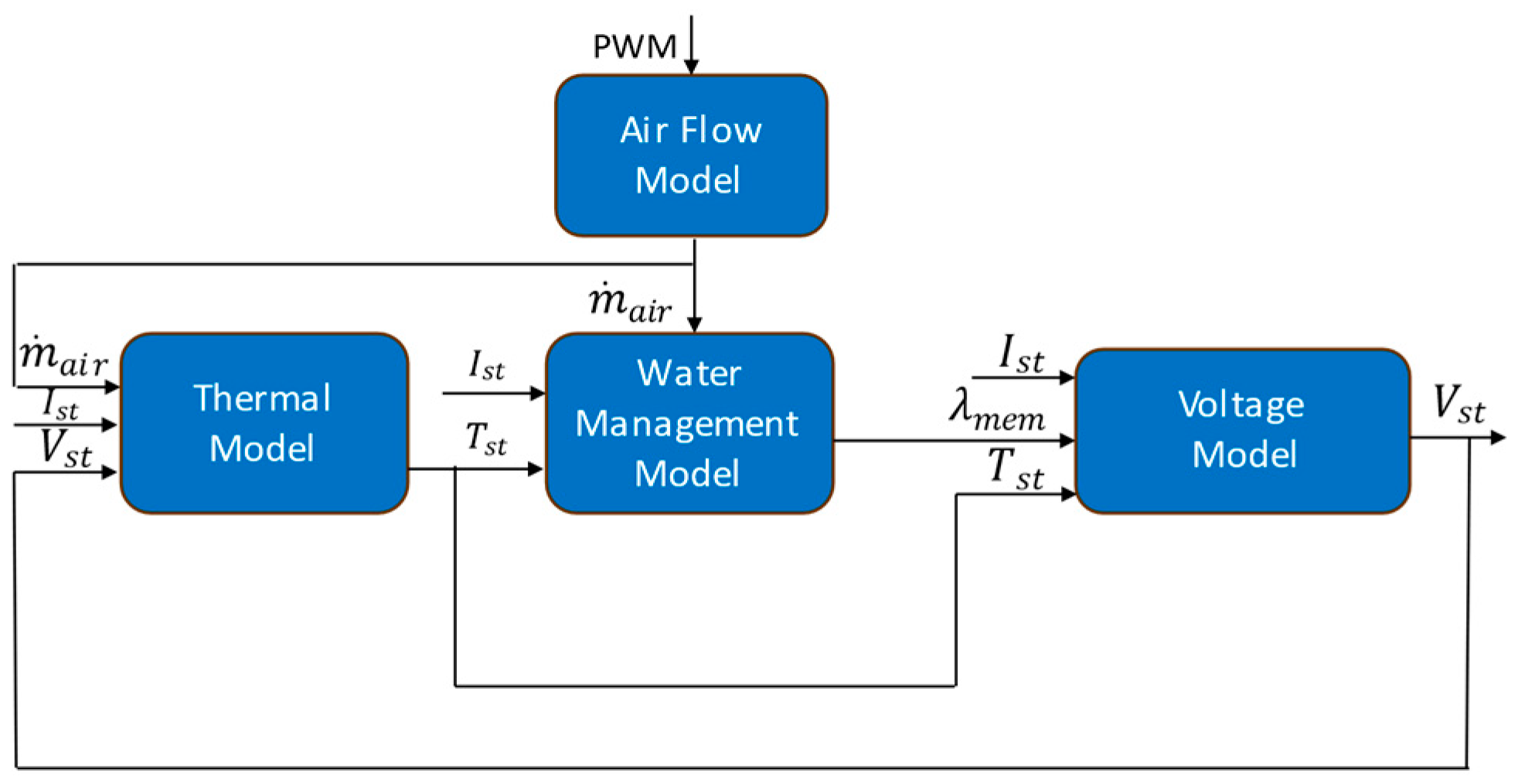
3. Model Development

3.1. Physics-Based Model

The model is made up of four interconnected sub-models. An air flow model computes the mass flow rate of air (${\dot{m}}_{air}$) from the fan’s PWM signal. The air flow rate is then fed into both the thermal and water management models. The thermal model generates the stack temperature $\left(T_{st}\right)$, which is used as an input to the water management and stack voltage models. The water management model’s prediction of membrane water content $\left({\lambda }_{mem}\right)$ then serves as an input to the stack voltage model. Figure 3 depicts the model’s structure.

3.1.1. Stack Voltage Model

The fuel cell reaction is split into the cathodic and anodic half reactions. To facilitate these reactions, air is supplied to the cathode, and hydrogen is supplied to the anode. The cathode and the anode are separated by the polymer electrolyte membrane, which is permeable to protons but not electrons, so electrons are transferred via an electrical circuit generating electric current. The electrons then recombine with the protons in the cathode side to generate water. Due to the transfer of electrons, the anodic reaction is referred to as the hydrogen oxidation reaction (HOR), and the cathodic reaction is called the oxygen reduction reaction (ORR) due to the addition of electrons. The electrochemical reactions involved are as follows:

$${\mathrm{H}}_2\to 2{\mathrm{H}}^{+}+2e^{-}\left(\mathrm{H}\mathrm{O}\mathrm{R},\mathrm{a}\mathrm{n}\mathrm{o}\mathrm{d}\mathrm{e}\right)$$

$$2{\mathrm{H}}^{+}+\frac{1}{2}{\mathrm{O}}_2+2e^{-}\to {\mathrm{H}}_2\mathrm{O}(\mathrm{O}\mathrm{R}\mathrm{R},\mathrm{c}\mathrm{a}\mathrm{t}\mathrm{h}\mathrm{o}\mathrm{d}\mathrm{e})$$

(1)

$${\mathrm{H}}_2+\frac{1}{2}{\mathrm{O}}_2\to {\mathrm{H}}_2\mathrm{O}(\mathrm{overall}\mathrm{reaction})$$

The voltage of a single cell is expressed by

$$V_{cell} \left(V\right)=V_{oc}-V_{act}-V_{ohmic}-V_{conc}$$

(2)

where $V_{oc}$ is the open circuit voltage, $V_{act }$ is the activation overvoltage, $V_{ohmic}$ is the ohmic overvoltage, and $V_{conc}$ is the concentration overvoltage.

$V_{oc}$ is the thermodynamic reversible potential or the fuel cell voltage when no load is connected. The reversible fuel cell voltage can be expressed as a function of temperature and pressure as follows [19]:

$$V_{oc}=E^o+\frac{∆s_{rxn}\left(T_{st}\right)}{nF}\left(T_{st}-T_{amb}\right)-\frac{R{T}_{st}}{nF}ln\left(\frac{1_{ }}{P{H}_2\ast P{O}_2^{0.5}}\right)$$

(3)

where $E^o$ is the non-standard reversible voltage, $∆s_{rxn}$ is the entropy change in the fuel cell reaction, $T_{st}$ is the stack temperature, $T_{amb}$ is the ambient temperature, $R$ is the ideal gas constant, $n$ is the number of moles of electrons transferred from the anodic reaction, $F$ is the Faraday constant, $P{H}_2$ is the hydrogen inlet pressure, and $P{O}_2$ is the oxygen partial pressure.

The activation overvoltage includes losses in voltage that arise due to the kinetic reaction. The activation overvoltage can be determined by

$$V_{act}=\frac{R{T}_{st}}{anF}ln \left(\frac{i}{i_o}\right)$$

(4)

where $a$ is the charge transfer coefficient, $i$ is the cell current density, and $i_o$ is the exchange current density.

The exchange current density can be computed by [16]

$$i_o=i_o^{ref}{\left(\frac{P{O}_2}{P_{ref}}\right)}^{y}exp\left[\frac{i}{i_o}\left(-\frac{E_c}{R}-\frac{1}{T_{ref}}\right)\right]$$

(5)

where $i_o^{ref}$ is the reference exchange current density, $P_{ref}$ is the reference pressure of 1 atm, $y$ is the pressure coefficient, $T_{ref}$ is the reference temperature of 298 K, and $E_c$ is the activation energy for the cathodic reaction. Due to the slower reaction kinetics of the ORR as compared to the HOR, the activation loss in this model is only attributed to the cathodic reaction.

Ohmic overvoltage captures the losses due to ionic and electronic conduction and can be calculated by

$$V_{ohmic}=i\left(R_{ionic}+R_{elec}\right)$$

(6)

where $R_{ionic}$ and $R_{elec}$ are the ionic resistance and electronic resistance, respectively. $R_{ionic}$ can be computed by [20]

$$R_{ionic}=\frac{181.6[1+0.03i+0.062{\left(\frac{T_{st}}{303}\right)}^2\left(i^{2.5}\right)]t_{mem}}{\left[{\lambda }_{mem}-0.634-3i\right]\exp [4.18\left(T_{st}-\frac{303}{T_{st}}\right)]}$$

(7)

in which $t_{mem}$ is the membrane thickness and ${\lambda }_{mem}$ is the membrane water content determined from the water management model as discussed in Section 3.1.4.

The concentration overvoltage includes losses attributed to mass transport in the fuel cell stack. The concentration overvoltage can be determined by

$$V_{conc}=mexp\left(ni\right)$$

(8)

where $m$ and $n$ are empirical coefficients that can be tuned according to experimental polarization data.

The total stack voltage is then computed by

$$V_{st}=V_{cell}\ast N_{st}$$

(9)

where $V_{cell}$ is the voltage of a single cell as computed from Equation (2) and $N_{st}$ is the total number of cells in the stack.

3.1.2. Air Flow Model

Air is delivered to the cathode channels via fans mounted on the stack casing. The flow to the cathode channel is assumed to be laminar in this model. The cathode air mass flow rate is modeled as

$${\dot{m}}_{air}\left(t\right)={\rho }_{air}\ast Q_{air}\left(t\right)$$

(10)

where ${\rho }_{air}$ is the density of air in kg/m³ at Standard Temperature and Pressure (STP) and $Q_{air}\left(t\right)$ is the volumetric air flow rate in m³/s.

For an arbitrary fan rotational speed, $Q_{air}\left(t\right)$ is determined by [21]

$$Q_{air}\left(t\right)=w\left(t\right)\frac{Q_{nom}}{w_{nom}}$$

(11)

where $w\left(t\right)$ denotes the arbitrary fan speed in revolutions per minute (rpm), $Q_{nom}$ is the nominal volumetric flow rate of the fan in m³/s, and $w_{nom}$ is the nominal fan speed in rpm. $Q_{nom}$ and $w_{nom}$ are determined in a manner as described by [22]. The pressure drop in the cathode channel is calculated as a function of the Reynolds number and friction factor. $Q_{nom}$ is then determined from the intersection of the determined pressure drop on the fan performance curve. $w_{nom}$ is the speed at which the performance curve is expressed in the datasheet. For this study, $w_{nom}$ is 6500 rpm.

3.1.3. Thermal Model

The thermal dynamics of the stack can be described as follows [22]

$$C_t\frac{d{T}_{st}}{dt}=P_{total}\left(t\right)-P_{st}\left(t\right)-{\dot{Q}}_{coolant}(t)$$

(12)

where $C_t$ represents the thermal capacitance of the stack and $P_{total}\left(t\right)$ is the power from the electrochemical reaction computed by

$$P_{total}\left(t\right)=\frac{N_{st}\ast I_{st}\left(t\right)\ast ∆h}{2F}$$

(13)

where $∆h$ is the molar enthalpy change in the electrochemical reaction. $P_{st}\left(t\right)$ is the total output power from the stack determined by

$$P_{st}\left(t\right)=V_{st}\left(t\right)\ast I_{st}\left(t\right)$$

(14)

${\dot{Q}}_{coolant}(t)$ is the heat dissipated from the air to the environment and it is calculated by

$${\dot{Q}}_{coolant}\left(t\right)={\eta }_{fan}\ast {\dot{m}}_{air}\left(t\right)\ast C_p(T_{st}\left(t\right)-T_{amb})$$

(15)

where ${\eta }_{fan}$ is the efficiency of the blower, ${\dot{m}}_{air}\left(t\right)$ is the air mass flow rate as determined from Section 3.1.2, $C_p$ is the specific heat capacity of air, and $T_{amb}$ is the ambient temperature.

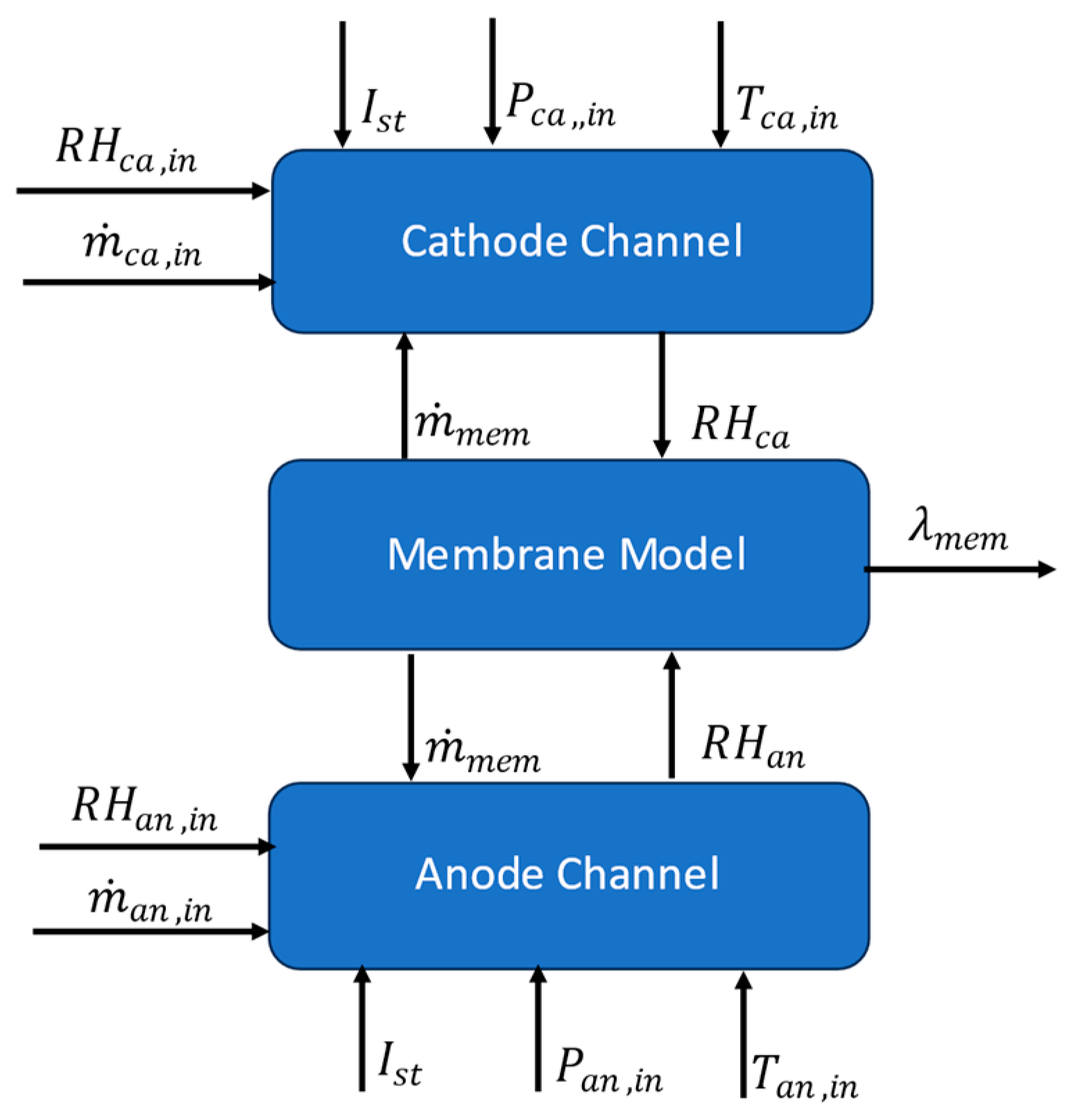
3.1.4. Water Management Model

The water management model is divided into three submodels: the cathode channel, the anode channel, and the polymer electrolyte membrane. A block diagram of the model is shown in Figure 4.

Cathode Channel

Conservation of mass was utilized to track the mass of species in the cathode channel over time. The conservation of mass of water, oxygen, and nitrogen are given by Equations (16)–(18), respectively [12]. It is assumed that water enters and leaves the channel in vapor form only.

$$\frac{d{m}_{H_{2}Oca}}{dt }={\dot{m}}_{H_2{O_{in},ca}_{ }}+{\dot{m}}_{H_2{O}_{gen}}-{\dot{m}}_{H_2{O_{out},ca}_{ }}+{\dot{m}}_{mem}$$

(16)

$$\frac{d{m}_{O_2}}{dt }={\dot{m}}_{{O_{2,in}}_{ }}-{\dot{m}}_{{O_{2,reacted}}_{ }}-+{\dot{m}}_{{O_{2,out}}_{ }}$$

(17)

$$\frac{d{m}_{N_2}}{dt }={\dot{m}}_{{N_{2,in}}_{ }}-{\dot{m}}_{{N_{2,out}}_{ }}$$

(18)

In these equations, ${\dot{m}}_{H_2{O_{in},ca}_{ }}$ ${\dot{m}}_{{O_{2,in}}_{ }}$ and ${\dot{m}}_{{N_{2,in}}_{ }}$ are the mass flow rates of water, oxygen, and nitrogen into the cathode channel, computed by Equations (24), (30) and (31), respectively. The mass flow rate of water vapor, oxygen, and nitrogen leaving the cathode channel is depicted by ${\dot{m}}_{H_2{O}_{out},ca}$, ${\dot{m}}_{{O_2,out}_{ }}$ and ${\dot{m}}_{{N_{2,out}}_{ }}$ and calculated by Equations (33), (43) and (44), respectively. The net flow of water across the membrane, ${\dot{m}}_{mem}$, is determined from the membrane model in Section Proton Exchange Membrane.

The water generated due to the electrochemical reaction is given by

$${\dot{m}}_{H_2{O}_{gen}}=\frac{N_{st}\ast I_{st}\ast {M_{H_{2}O}}_{ } }{\begin{array}{c}2F\\ \end{array}}$$

(19)

where $M_{H_{2}O}$ is the molar mass of water in kg/mol. The mass flow rate of oxygen that partakes in the electrochemical reaction computed by

$${\dot{m}}_{{O_{2,reacted}}_{ }}=\frac{N_{st}\ast I_{st}\ast {M_O}_2 }{4F}$$

(20)

in which ${M_O}_2$ is the molar mass of oxygen in kg/mol.

Anode Channel

Similar to the cathode channel, conservation of mass was utilized to track the mass of water and hydrogen in the anode channel. The anode of the self-humidifying open-cathode PEMFC under consideration is fed with dry hydrogen and it is typically dead-ended except for the occasional purging of water and unused hydrogen by the purge valve. It is assumed in this model that the anode runs exclusively in the dead-ended mode.

The mass balance of water is determined by

$$\frac{d{m}_{H_{2}Oan}}{dt }=-{\dot{m}}_{mem}$$

(21)

The mass balance of hydrogen is given by

$$\frac{d{m}_{H_2}}{dt}={\dot{m}}_{{{H_2}_{in,an}}_{ }}-{\dot{m}}_{{{H_2}_{out,an}}_{ }}-{\dot{m}}_{{H_2}_{reacted}}$$

(22)

The mass rate of hydrogen reaction is determined by

$${\dot{m}}_{{H_2}_{reacted}}=\frac{N_{st}\ast I_{st}\ast M_{H_2} }{2F}$$

(23)

The mass flow rate of water entering the channels is given by

$${\dot{m}}_{H_2{O_{in}\left(.\right)=x_{H_2{Ov}_{in}(.)}\ast {\dot{m}}_{in(.)}}_{ }}$$

(24)

where $(.)$ represents either the cathode (ca) or anode (an) channel. The term $x_{H_2{Ov}_{in}(.)}$ is the mass fraction of vapor in the inlet flow and ${\dot{m}}_{in}$ is the inlet flow rate. For the cathode channel, ${\dot{m}}_{in,ca}$ is determined from the air flow rate model in Section 3.1.2 and for the anode, and ${\dot{m}}_{in,an}$ is a measured input to the model.

The mass fraction of vapor in the channel is computed by [23]

$$x_{H_{2}Ovin(.)}=\frac{P_{H_{2}O{v}_{in}(.)}\ast M_{H_{2}Ov}}{\left(P_{H_{2}O{v}_{in}(.)}\ast M_{H_{2}Ov}\right)+\left(\right({P_{(.)}}_{in}-P_{H_{2}O{v}_{in}(.)})\ast M_g)}$$

(25)

The subscript, $g,$ represents the gas in the channel. For the cathode, the gas is air, and it is hydrogen for the anode.

The inlet vapor pressure is calculated by

$$P_{H_{2}O{v}_{in}(.)}=R{H_{(.)}}_{in}\ast P_{sat}\left({T_{(.)}}_{in}\right)$$

(26)

where $R{H_{(.)}}_{in}$ is the channel inlet relative humidity and $P_{sat}\left({T_{(.)}}_{in}\right)$ is the saturation pressure evaluated at the channel inlet temperature.

${P_{(.)}}_{in}$ is the channel inlet pressure and $M_g$ is the molar mass of gas in the channel. Once the mass flow rate of water in the inlet stream has been determined, the inlet flow rate of the gas is determined by subtracting the water mass flow rate from the total inlet flow rate.

$${\dot{m}}_{g_{in(.)}}={\dot{m}}_{in(.)-}{\dot{m}}_{H_2{O}_{in},(.)}$$

(27)

To determine the mass flow rate of each of the nitrogen and oxygen species in the cathode, the mass fraction of each of the gases needs to be computed and this is given by [12].

$$x_{O_2}c{a}_{in}=\frac{y_{O_2}c{a}_{in}\ast M_{O_2}}{(y_{O_2}c{a}_{in}\ast M_{O_2})+(\left(1-y_{O_2}c{a}_{in}\right)\ast M_{N_2})}$$

(28)

where $y_{O_2}c{a}_{in}$ is the mole fraction of the oxygen in the inlet air which is 0.21.

The mass fraction of nitrogen is then given by

$$x_{N_2}c{a}_{in}=1-x_{O_2}c{a}_{in}$$

(29)

The mass flow rate of oxygen into the cathode is

$${\dot{m}}_{{O_2}_{in.ca}}=x_{O_2}c{a}_{in}\ast {\dot{m}}_{{air}_{in,ca}}$$

(30)

and the mass flow rate of nitrogen is

$${\dot{m}}_{{N_2}_{in,ca}}=x_{N_2}c{a}_{in}\ast {\dot{m}}_{{air}_{in,ca}}$$

(31)

The outlet flow rate is determined from the linearized nozzle equation [23]

$${\dot{m}}_{ou{t}_{(.)}}={k_{\left(.\right)}}_{out}(P_{\left(.\right)}-P_{ds})$$

(32)

in which ${k_{\left(.\right)}}_{out}$ is the outlet anode or cathode nozzle constant coefficient, $P_{\left(.\right)}$ is the anode or cathode channel pressure, and $P_{ds}$ is the pressure downstream of the stack, and for the lumped model, this is equal to standard atmospheric pressure.

Knowing the outlet flow rate, the mass flow rate of vapor going out can be computed by

$${\dot{m}}_{H_2{O}_{out}\left(.\right)=}{x}_{H_2{O}_v(.)}\ast {\dot{m}}_{out(.)}$$

(33)

The mass fraction of water vapor is given by

$$x_{H_{2}Ov\left(.\right)}=\frac{m_{H_{2}Ov\left(.\right)}}{m_{H_{2}Ov\left(.\right)}+m_g\left(.\right)}$$

(34)

where $m_{H_{2}Ov(.)}$ and $m_g\left(.\right)$ are the masses of vapor and gas, respectively, in the cathode or anode channel. The total mass of gas in the cathode channel is obtained by summing the masses of nitrogen and oxygen.

Based on the calculated quantity of water exiting, the amount of gas going out of the channels can be computed by

$${\dot{m}}_{{g_{out,(.)}}_{ }}={\dot{m}}_{ou{t}_{(.)}}-{\dot{m}}_{H_2{O}_{out}(.)}$$

(35)

To determine the flow rate of the individual species of nitrogen and oxygen going out of the cathode, the mass fractions have to be recomputed as oxygen is consumed in the reaction.

The mass fraction of oxygen leaving the cathode is [12]

$$x_{O_2}=\frac{y_{O_2}\ast M_{O_2}}{(y_{O_2}\ast M_{O_2})+(\left(1-y_{O_2}\right)\ast M_{N_2})}$$

(36)

where $y_{O_2}$ is the mole fraction of oxygen in the exit flow rate and it is determined by

$$y_{O_2}=\frac{P_{O_2}}{Pai{r}_{ }}$$

(37)

Assuming the gases to be ideal, the partial pressures of oxygen and nitrogen in the cathode channel are determined from the ideal gas law as

$$P_{O_2}=\frac{m_{O_2}\ast R_{O_2}\ast T_{ca} }{V_{ca}}$$

(38)

$$P_{N_2}=\frac{m_{N_2}\ast R_{N_2}\ast T_{ca} }{V_{ca}}$$

(39)

where $m_{O_2}$ and $m_{N_2}$ are the masses of oxygen and nitrogen obtained by solving Equations (17) and (18), respectively. $R_{O_2}$ is the gas constant of oxygen and $R_{N_2}$ is the gas constant of nitrogen. $T_{ca}$ is the cathode channel temperature and it is taken to be the same as the stack temperature $\left(T_{st}\right)$ in this study. $V_{ca}$ is the lumped volume of the cathode channel.

Similarly, the partial pressure of hydrogen in the anode channel is calculated by

$$P_{H_2}=\frac{m_{H_2}\ast R_{H_2}\ast T_{an} }{V_{an}}$$

(40)

where $m_{H_2}$ is the mass of hydrogen found in Equation (22), $R_{H_2}$ is the hydrogen gas constant, $T_{an}$ is the anode temperature, which is equal to $T_{st}$ in this model, and $V_{an}$ is the lumped anode channel volume.

The partial pressure of air in the channel is then given by the summation of Equations (38) and (39) as

$$P_{air}=P_{O_2}+P_{N_2}$$

(41)

The mass fraction of nitrogen in the exit flow rate is

$$x_{N_2}=1-x_{O_2}$$

(42)

Knowing the mass fraction of oxygen and nitrogen in the exit flow rate, the exit mass flow rate of oxygen and nitrogen can then be determined from Equations (43) and (44), respectively.

$${{{\dot{m}}_{O_2}}_{out}}_{ca}=x_{O_2}\ast {\dot{m}}_{ai{r}_{out}}$$

(43)

$${{{\dot{m}}_{N_2}}_{out}}_{ca}=x_{N_2}\ast {{\dot{m}}_{air}}_{out}$$

(44)

If the mass of water in the channels computed from Equations (16) and (21) is greater than the maximum amount of vapor the gas can hold (saturation mass), the extra amount is assumed to condense into liquid form instantaneously. The saturation mass is computed from

$$m_{sat\left(.\right)}=\frac{P_{sat}\left(T_{st}\right)\ast V(.)}{R_{H_{2}Ov}\ast T_{st}}$$

(45)

where $V\left(.\right)$ is the lumped volume of the anode or cathode channel and $P_{sat}\left(T_{st}\right)$ is the saturation pressure and can be determined as a function of $T_{st}$ by

$$log{P}_{sat}=-5.609\ast {10}^{-10}{T}_{st}^4+9.8172\ast {10}^{-7}{T}_{st}^3-6.7687\ast {10}^{-4}{T}_{st}^2+0.22471T_{st}-28.365$$

(46)

where $T_{st}$ is in K and the calculated $P_{sat}$ is in kPa. The relative humidity inside the channels is then calculated by

$$RH(.)=\frac{P_{H_2{O}_v\left(.\right)}}{P_{sat}\left(T_{st}\right)}$$

(47)

where $P_{H_2{O}_v\left(.\right)}$ is the partial pressure of water vapor in the channel and is given by

$$P_{H_2{O}_v\left(.\right)}=\frac{m_{H_2{O}_v(.)}\ast R_{H_2{O}_v}\ast T_{st} }{V(.)}$$

(48)

where $m_{H_2{O}_v}$ is the minimum of the dynamically computed mass and the saturation mass. For the anode, $m_{H_2{O}_v}$ is the minimum of Equations (21) and (45). For the cathode, it is the minimum of Equations (16) and (45).

The total anode and cathode channel pressures are then determined by Equations (49) and (50), respectively:

$$P_{an}=P_{H_2}+P_{H_2{O}_{v}an}$$

(49)

$$P_{ca}=P_{air}+P_{H_2{O}_{v}ca}$$

(50)

Proton Exchange Membrane

Water is transported across the PEM fuel cell membrane by two main phenomena: electro-osmotic drag (EOD) and back diffusion. As protons move from the anode, they drag water molecules along and this is termed as EOD. This causes a water gradient to form, causing a back diffusion of water from the cathode to the anode.

The net mass flow rate of water across the membrane is given by [24]

$${\dot{m}}_{mem}=M_{H_2{O}_v}\ast A_{fc}\ast N_{st}\ast (\frac{n_d\ast i}{F}-D_w\frac{\left(C{v}_{ca}-C{v}_{an}\right)}{tmem})$$

(51)

where $n_d$ is the electroosmotic drag coefficient, $D_w$ is the diffusion coefficient, $C{v}_{ca}$ is the concentration of water in the cathode, and $C{v}_{an}$ is the concentration of water in the anode. The first term, $\frac{nd\ast i}{F},$ represents the molar rate of EOD, and the second term, $D_w\frac{(C{v}_{ca}-C{v}_{an})}{tmem},$ represents the molar rate of water vapor via back diffusion.

The electroosmotic drag is determined by [25]

$$n_d=\frac{2.5\ast {\lambda }_{mem}}{22}$$

(52)

The water concentrations in the cathode and anode are given by Equations (53) and (54), respectively:

$$C{v}_{ca}=\frac{{\rho }_{mem}}{M_{mem}}\ast {\lambda }_{ca}$$

(53)

$$C{v}_{an}=\frac{{\rho }_{mem}}{M_{mem}}\ast {\lambda }_{an}$$

(54)

where ${\rho }_{mem}$ and $M_{mem}$ are the membrane dry density and dry equivalent weight, respectively, and ${\lambda }_{ca}$ and ${\lambda }_{an}$ are the water content in the cathode and anode channels, respectively. The water content is defined as the number of water molecules per sulfonic acid site and is determined by the following empirical relation [25]

$${\lambda }_{\left(.\right)}=\left\{\begin{array}{c} \\ \begin{array}{c}0.043+17.81RH\left(.\right)-39.85RH{\left(.\right)}^2+36RH{\left(.\right)}^3, 0<RH\left(.\right)\le 1\\ 14+1.4\left(RH\left(.\right)-1\right), 1<RH\left(.\right)\le 3\\ \end{array}\end{array}\right.$$

(55)

where the subscript (.) represents either the membrane (mem), cathode (ca), or anode (an), and $RH$ is the relative humidity.

The relative humidity of the membrane is modeled as the average of the cathode and anode relative humidities.

$$R{H}_{mem}=\frac{({RH}_{ca}+R{H}_{an})}{2}$$

(56)

The diffusion coefficient is expressed by

$${D_w=D}_{\lambda }\exp (2416(\frac{1}{303}-\frac{1}{T_{st}}))$$

(57)

in which

$$D_{\lambda }=\left\{ \begin{array}{c}{10}^{-6}, {\lambda }_{mem}<2 \\ {10}^{-6}\left(1+2\left({\lambda }_{mem}-2\right)\right),2 \le {\lambda }_{mem}\le 3\\ {10}^{-6}\left(3-1.67\left({\lambda }_{mem}-3\right)\right), 3 \le {\lambda }_{mem}\le 4.5 \\ 1.25\times {10}^{-6},{\lambda }_{mem}\ge 4.5\end{array} \right.$$

(58)

Together, these submodels allow the water content in the stack to be monitored.

3.2. GT-Suite Model

The fuel cell stack was modeled in GT Suite v2023 using the stack’s specification. The model was calibrated using experimental voltage and temperature data. Throughout the GT modeling process, a steady inlet hydrogen tank pressure was assumed. In addition, the cathode’s input was a scaled version of the air mass flow rate that was determined in Section 3.1.2, which was optimized to provide accurate voltage predictions. The model, like the experimental PEM fuel cell stack, is devoid of a separate cooling channel. A heat transfer multiplier (HTM) is utilized in its place to account for cooling.

4. Model Discretization

4.1. Physics-Based Model

To predict localized effects, the lumped model was divided into four control volumes (CVs), each with 30 cells, and the output of each CV was fed into the next in order to capture variations in membrane water content along the fuel cell stack. The choice of the number of CVs was contingent upon experimental data available for model validation. More details on the validation of the model are covered in Section 5.2. The governing equations remain unchanged from the lumped model, with slight modifications made to specific equations to account for the subdivision.

In discretization, a co-flow technique in which the fuel and air both flow in the same direction was employed. The inlet flow to CV1 is the same as the inlet flow to the lumped model. Subsequent CVs, however, receive their inlet flows from the outlet of the CV immediately preceding it. The outlet flow is determined by using the linearized nozzle equation in (32) which is adjusted as

$${\dot{m}}_{{ou{t}_{\left(cvi\right)}}_{ }}={k_{ca}}_{out}(P_{cvi}-P_{cv(i+1)})$$

(59)

where $P_{cvi}$ is the total pressure of the current CV cathode channel and $P_{cv(i+1)}$ is the total pressure of the subsequent CV, which is the downstream pressure. For the last CV, $P_{cv(i+1)}$ is equal to the standard atmospheric pressure.

For the anode, it is assumed that the mass flow controller is able to regulate the flow such that pressure differences in the channel are kept to a minimum. As a result, the flow rate to each CV remains unchanged. To guarantee that there is sufficient flow of oxygen for the fuel cell reaction to occur, the anode channel is assumed to have a low flow resistance. Due to this low resistance, the mass flow controller can regulate the flow without significant pressure variation.

Regarding the stack voltage model, the number of cells was modified to reflect the number of cells in a CV rather than the whole stack. The voltage output for each CV was then determined by

$${\mathrm{V}}_{{st,c{v}_i}_{ }}=V_{cell}\ast {N_{cells}}_{c{v}_i}$$

(60)

where $V_{cell}$ was computed by Equation (2) as described in Section 3.1.1 and ${N_{cells}}_{c{v}_i}$ is the number of cells in the control volume.

The total stack voltage is then computed by adding the voltages in each CV

$${\mathrm{V}}_{{st}_{ }}=V_{st,cv1}+V_{st,cv2}+V_{st,cv3}+V_{st,cv4}$$

(61)

With regard to the discretization of the temperature dynamics model, the efficiency of the fan, ${\eta }_{fan},$ in Equation (15) was optimized at each current input for each CV using Simulink’s parameter estimation feature in the design optimization toolbox to align the model’s prediction with experimental data.

For the water management model, each CV had a distinct thermal subsystem to account for the temperature variations. Also, the anode and cathode channel volumes were divided according to the number of cells in each CV. Another modification to the discretized water management model is that while the anode is fed with dry hydrogen, this was solely the case for CV1. Back diffusion from the cathode channel results in humid hydrogen entering subsequent CVs. This inlet relative humidity is the output relative humidity from the previous CV which is computed by Equation (47).

4.2. GT-Suite Model

The developed GT-Suite model was discretized by applying the same method used to discretize the lumped physics-based model. The GT-Suite model was discretized using four distinctive fuel cell stacks, one for each control volume. The input for the first stack was the known measured input, much like the physics-based model, and the input for successive stacks was the output of the stack preceding it. Each stack’s thermal and electrical domains were also appropriately linked. The thermocouple readings were used to calibrate each stack of the discretized model. Similar to the lumped model, the HTM was applied to account for cooling and the HTM used for each stack was iteratively optimized to match the temperature to the experimental thermocouple reading.

5. Results and Discussion

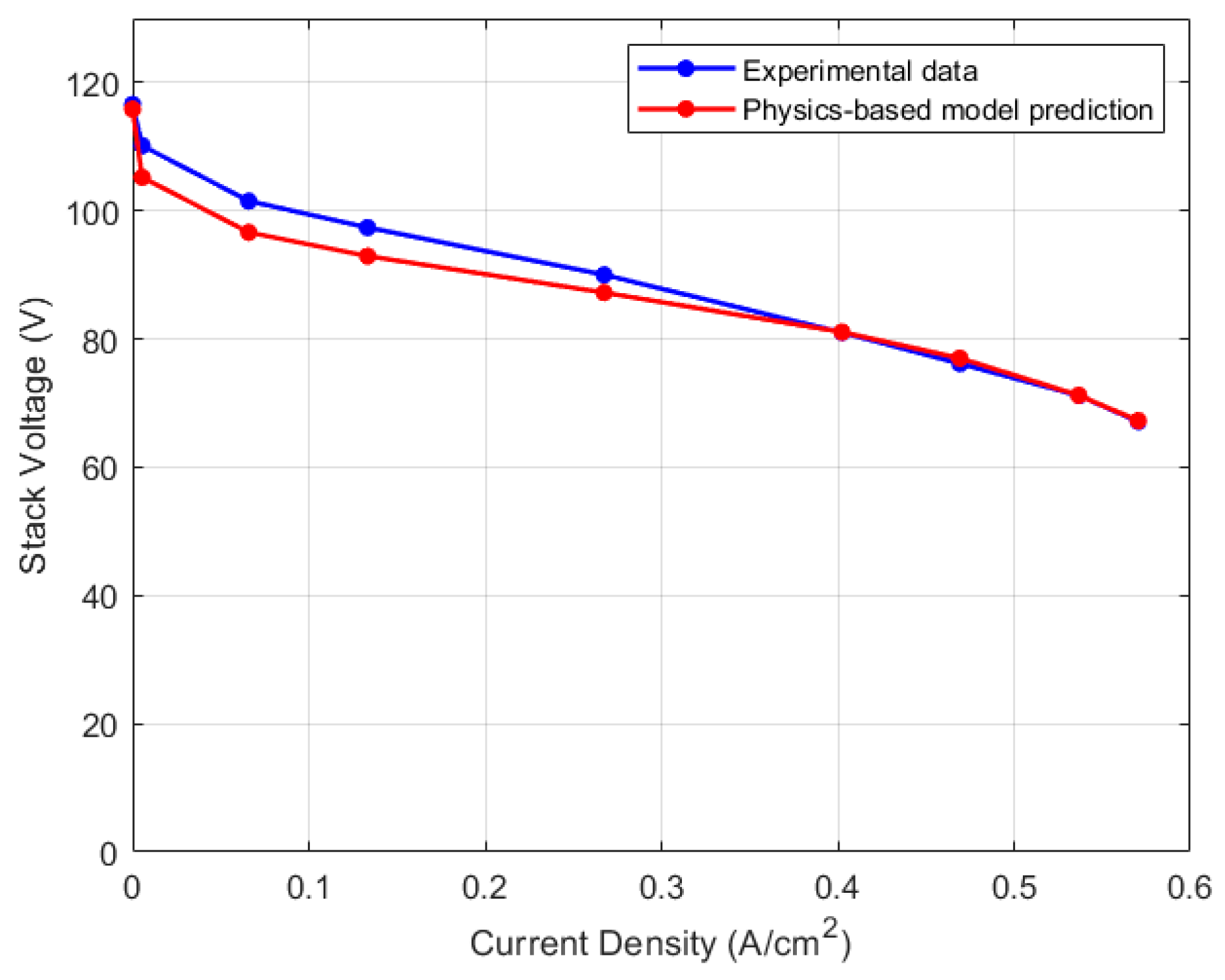
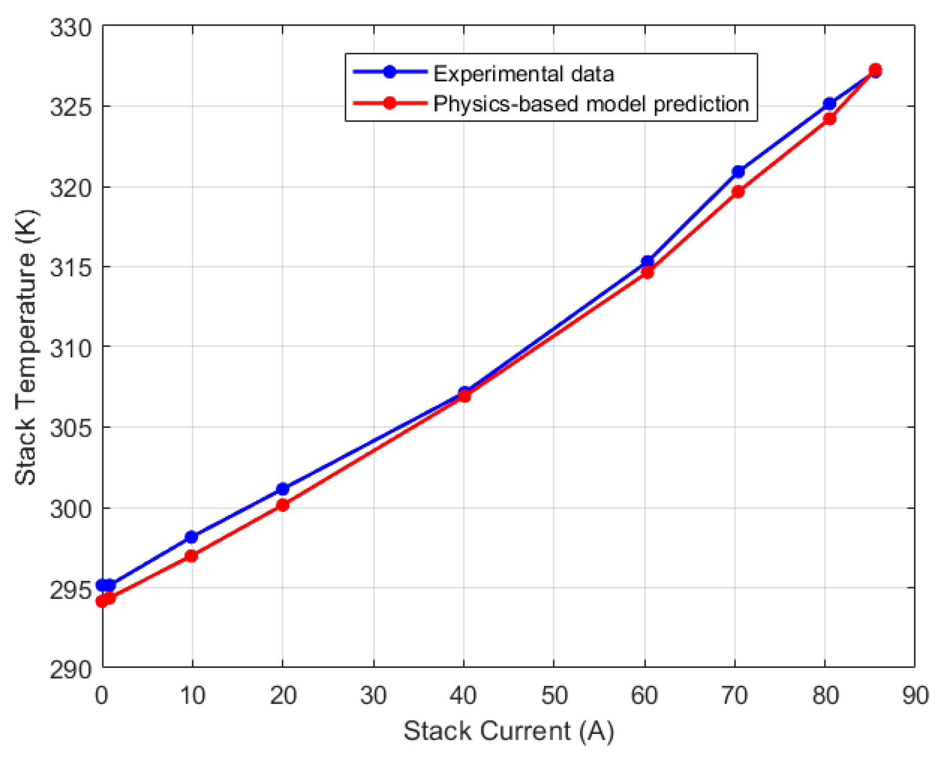
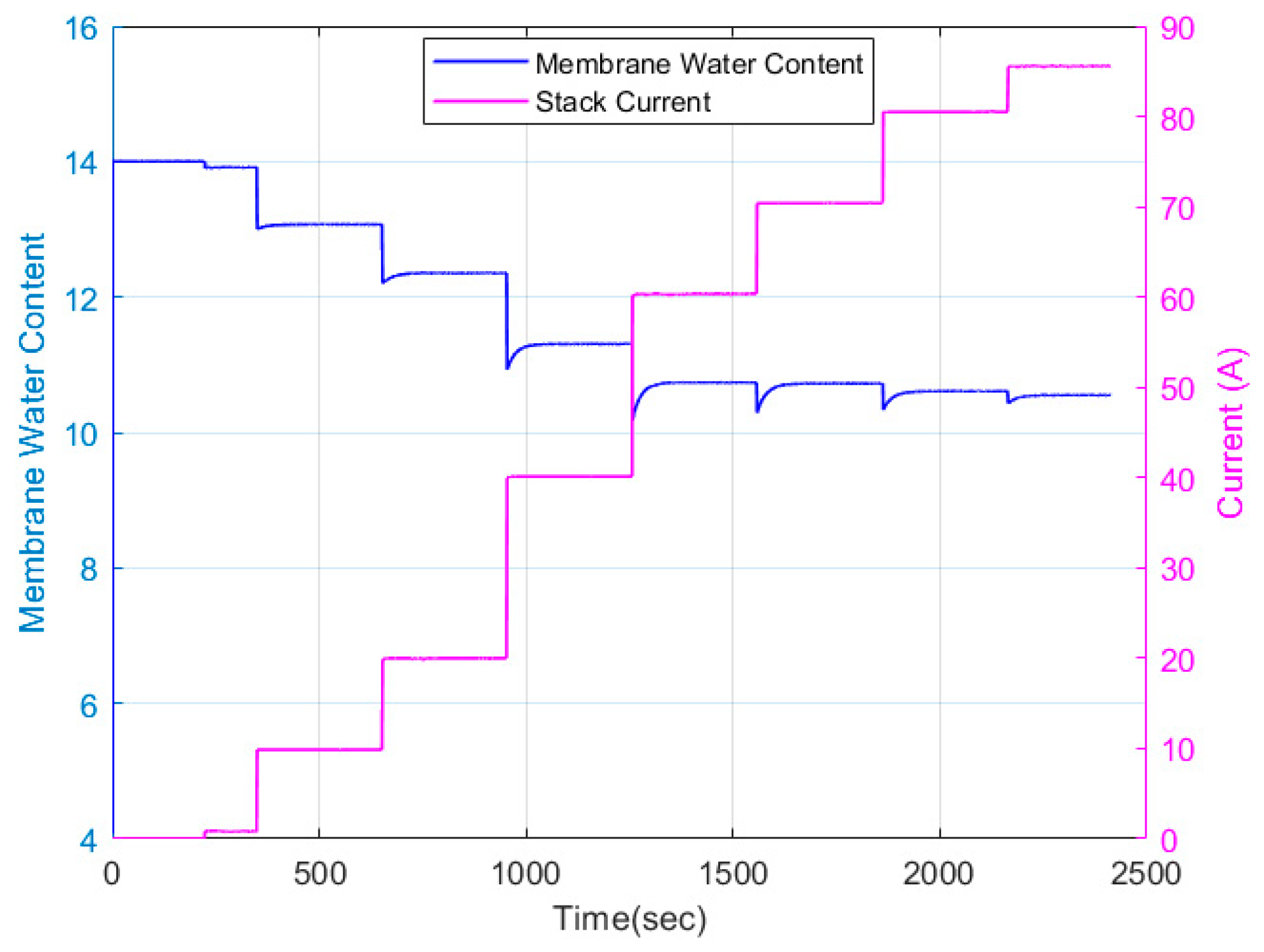
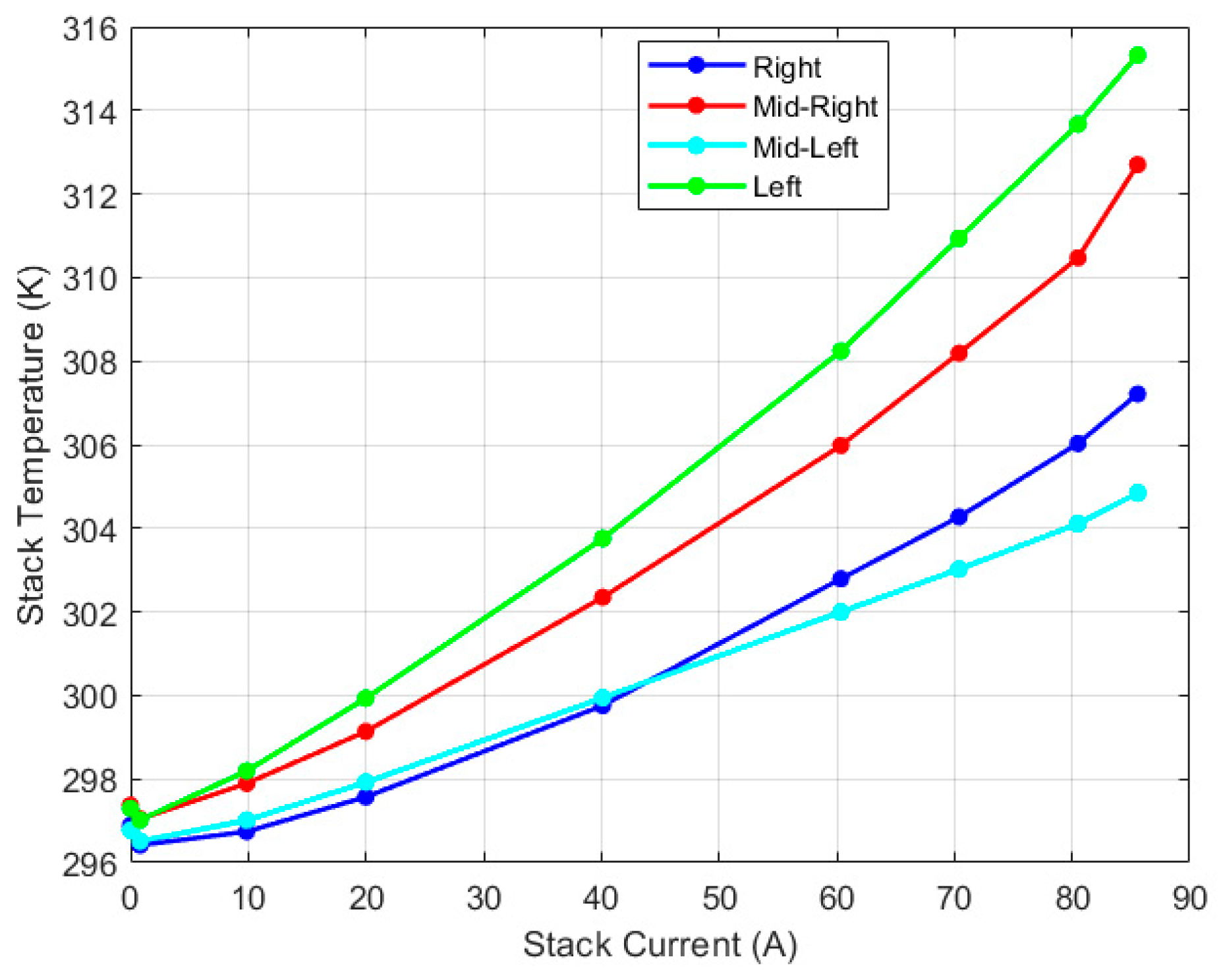
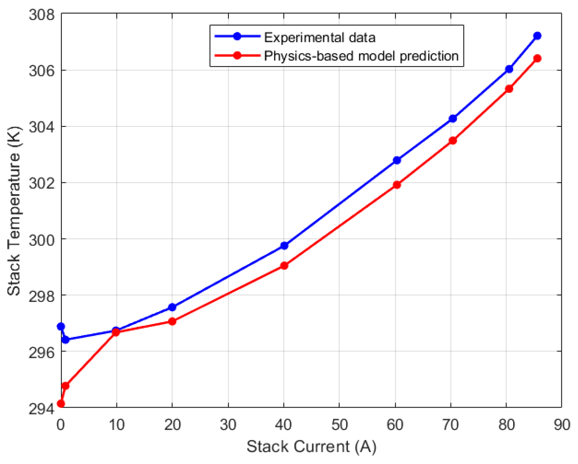
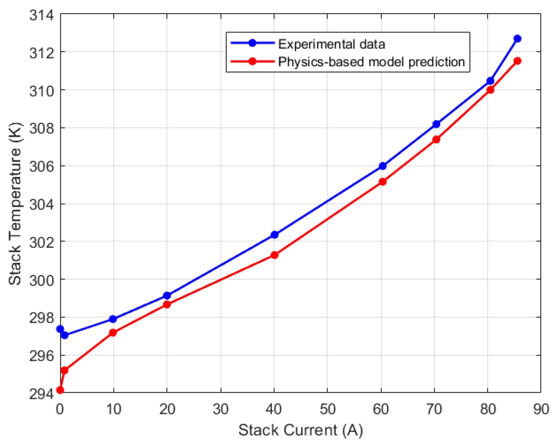
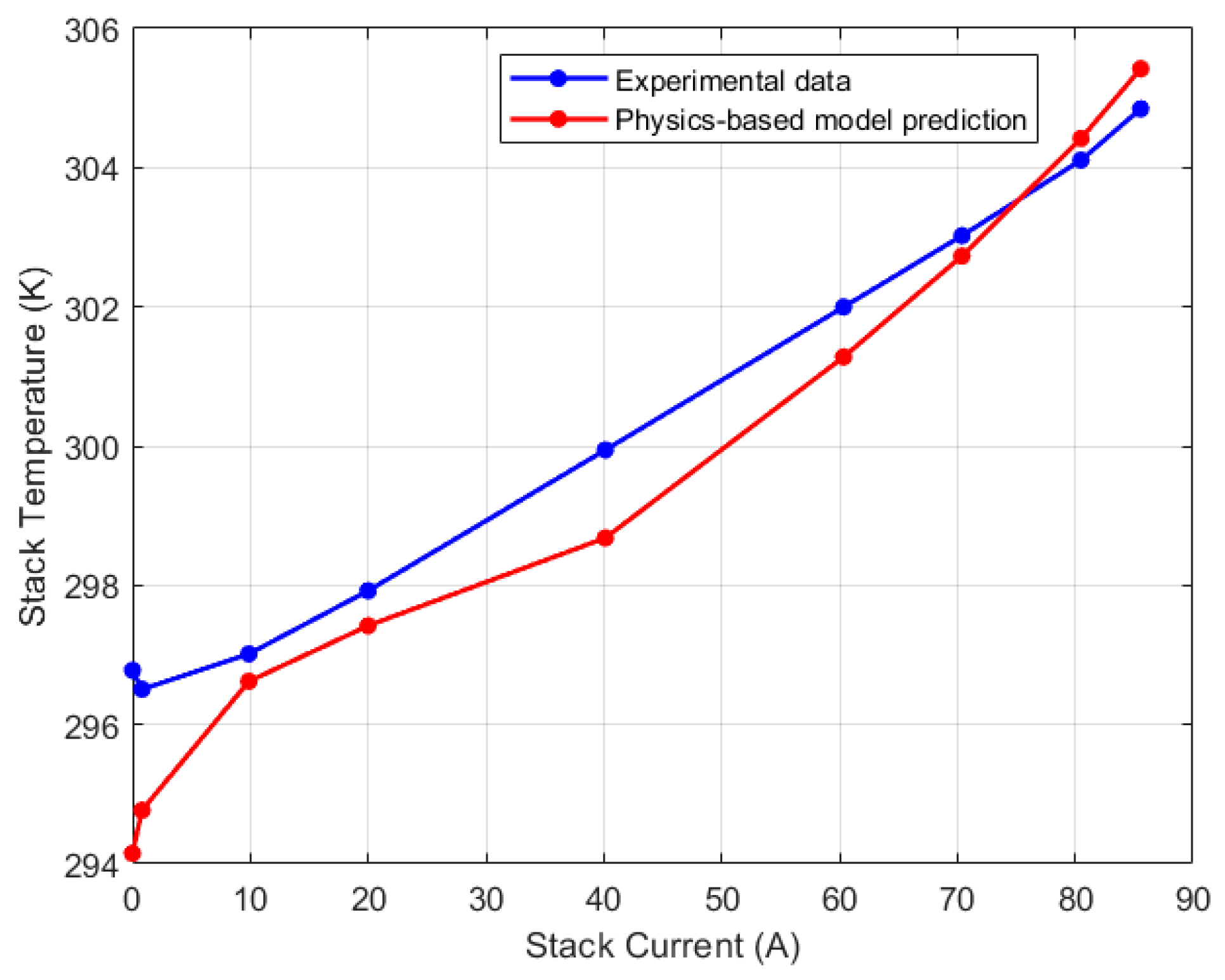
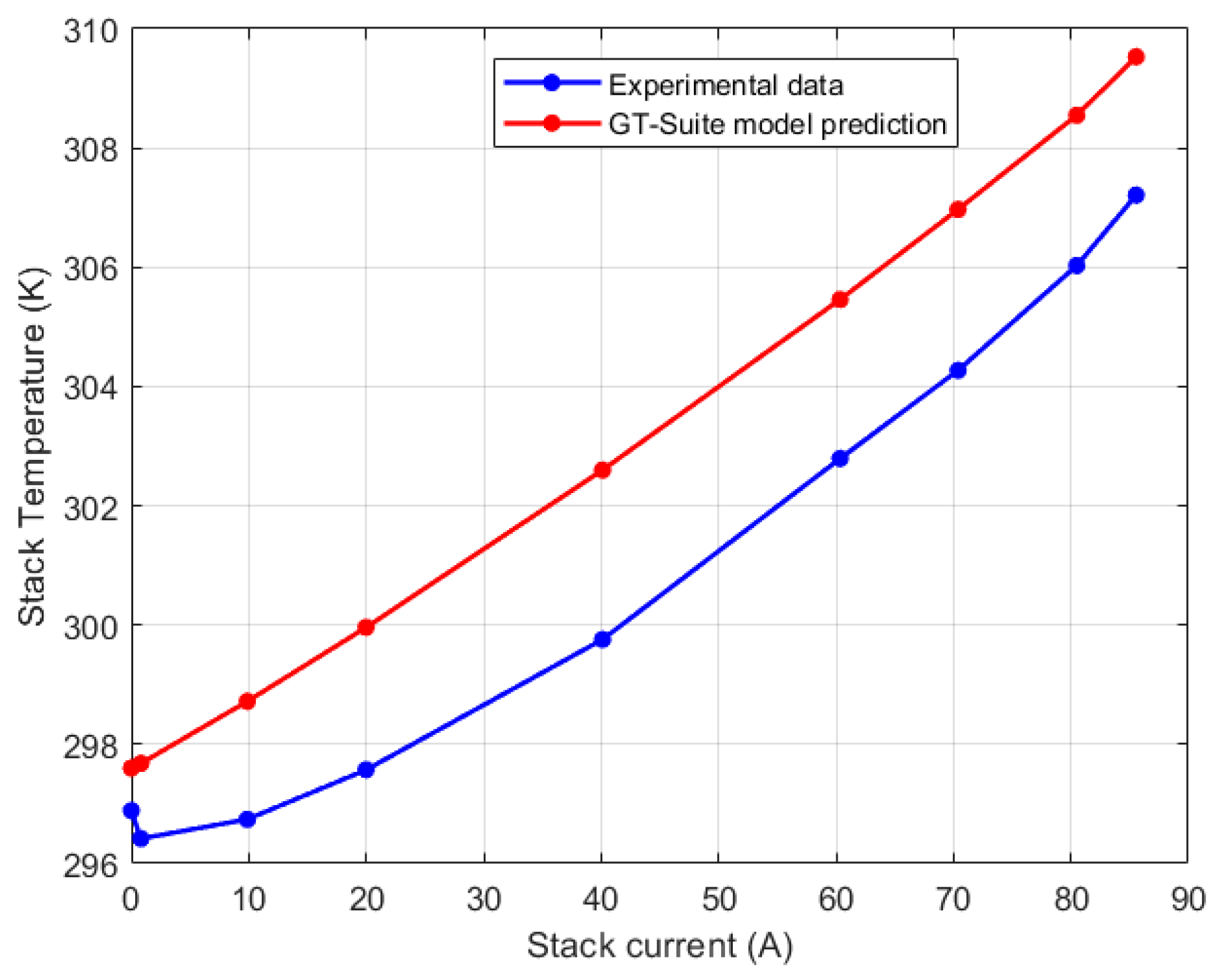
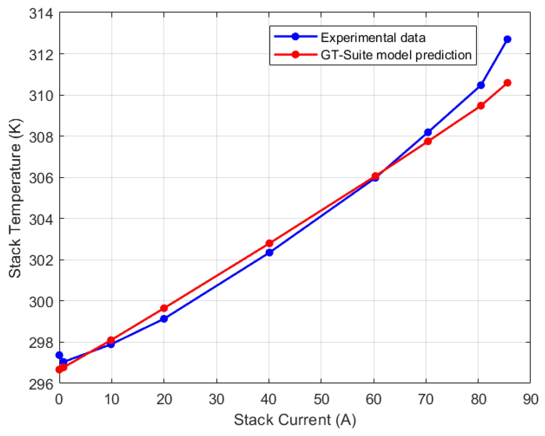
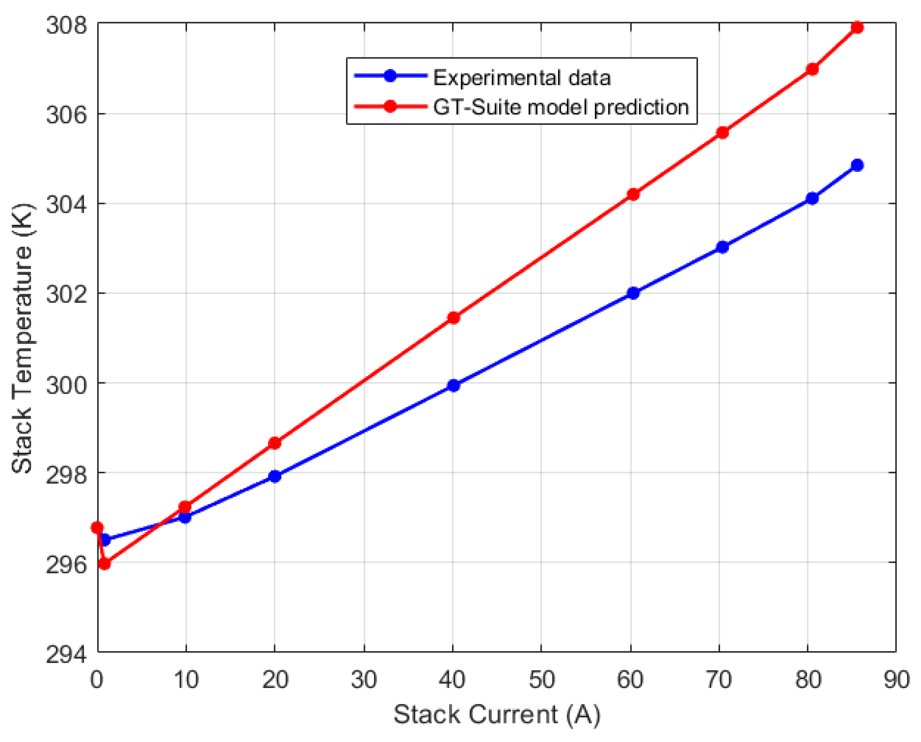
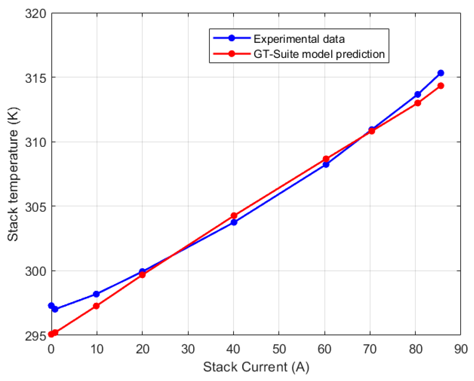
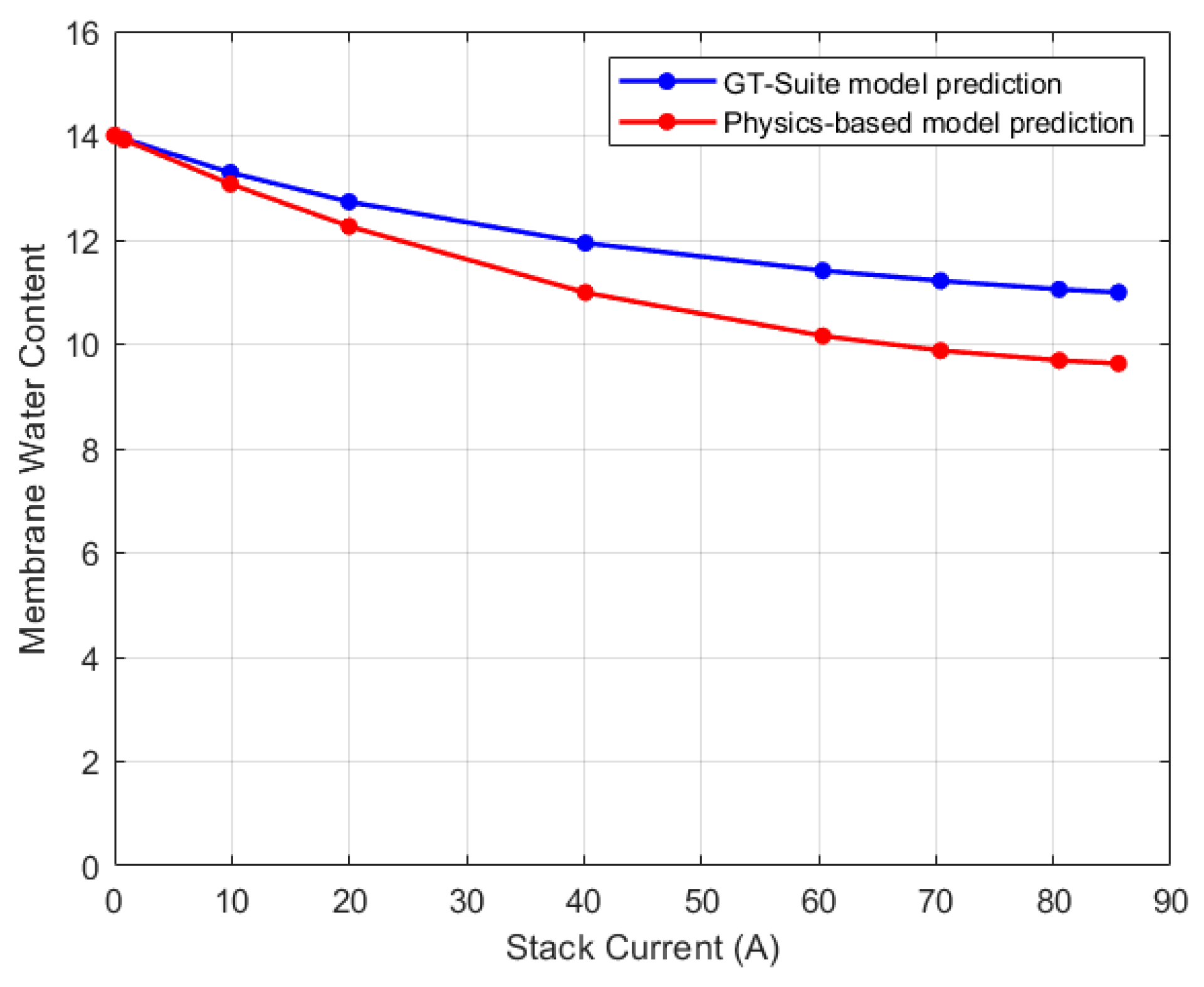
5.1. Lumped Model Validation

The stack voltage and thermal models were validated using data from the experimental setup as described in Section 2. Figure 5 highlights the steady state calibration result for the physics-based stack voltage model where errors are within 5% of the experimental data. The calibration results for the lumped thermal model are depicted in Figure 6. The fan efficiency was used as a tuning parameter in the thermal model calibration. In Simulink, an optimization search for best efficiency was carried out, and an optimal efficiency of 35.75% was reached. When compared to the experimental data, the maximum steady state error for the thermal model is only 0.4%, highlighting the model’s accuracy in predicting the stack temperature.

Due to the lack of experimental data to validate the water management model’s prediction, the simulation results from the GT-Suite model provided a basis for comparison. The GT-Suite model was calibrated using the experimental voltage and temperature data and the results are shown in Figure 7 and Figure 8, respectively, with a maximum relative error of 2.38% for the voltage model and 0.81% for the thermal model.

After validating the thermal and voltage predictions of GT-Suite, its membrane water content was used to validate the physics-based water management model. The comparison results are shown in Figure 9. The root mean square error (RMSE) between the predictions was found to be 0.72 membrane water content. Notably, the GT-Suite model predicted higher water content for all current cases than the physics-based model. One plausible explanation for this could be due to the temperature predictions of the GT-Suite model. For current inputs ranging from 0 A to 40 A, the GT-Suite model overestimates the stack temperature which could lead to an increase in water content. On the contrary, for these same current values, the physics-based model slightly underestimates the stack temperature. The discrepancy in the predictions could be due to variations in the models’ initialization. Even though the GT-Suite model underestimates the water content from 60 A to 85 A, the water content remains high. This could be due to water saturation as a result of increasing water generation in these high current zones. As a result, despite the modest shift in the trend of stack temperature, the water content may remain elevated.

The membrane water content dynamics from the physics-based model are shown in Figure 10. As can be observed, an increase in current input leads to a decrease in the membrane water content. In their work regarding modeling humidity dynamics of an open-cathode PEM fuel cell, Chen et al. [16] observed similar dynamics of membrane water content in response to an increase in current. Karthik and Vijayachitra [26] and Chen et al. [15] also reported a decrease in membrane water content with increasing current density. The dynamics of the membrane water content are influenced by the relative humidity dynamics in the anode and cathode channels as depicted in Figure 11. The cathode relative humidity remains constant at 100% in all current cases due to water generation at the cathode electrode. The relative humidity of the anode channel, however, decreases with an increase in current. This can be due to an increase in electroosmotic drag from the anode to the cathode channel. This observation of the relative humidity dynamics in the anode and cathode channels is corroborated by the work of Zhang and Zhou [27]. Falcão et al. [28] and Karnik et al. [23] also reported a decrease in anode water content with an increase in current. The parameters used for the simulation of the models are shown in

Table 2. Parameters used in model simulation.

Symbol	Variable	Value
$A_{fc}$	Active area of fuel cell	150 cm2
$N_{st}$	Number of cells in stack	120
$F_{ }$	Faraday constant	96,485 Coulombs
$t_{mem}$	Membrane thickness	0.0035 cm
$R_{ }$	Ideal gas constant	8.314 J/(mol·K)
${{R_{H_{2}O}}_v}_{ }$	Water vapor gas constant	461.5 J/(kg·K)
$R_{O_2}$	Oxygen gas constant	259.8 J/(kg·K)
$R_{N_2}$	Nitrogen gas constant	296.9 J/(kg·K)
$R_{H_2}$	Hydrogen gas constant	4124.3 J/(kg·K)
${{M_{H_{2}O}}_v}_{ }$	Water vapor molar mass	0.018 kg/mol
$M_{O_2}$	Oxygen molar mass	0.032 kg/mol
$M_{N_2}$	Nitrogen molar mass	0.028 kg/mol
$M_{H_2}$	Hydrogen molar mass	0.002 kg/mol
$n_{ }$	No. of electrons transferred	2
$k_{ca,out}$	Cathode outlet flow coefficient	$2.2\times {10}^{-6}$ kg/(s·Pa)
$V_{an}$	Anode volume per cell	$2.58\times {10}^{-6}$ m3
$V_{ca}$	Cathode volume per cell	$2.59\times {10}^{-5}$ m3
${\rho }_{mem}$	Membrane dry density	0.002 kg/cm3
$M_{mem}$	Membrane equivalent weight	1.1 kg/mol
$C_p$	Specific heat capacity of air	1006 J/(kg·K)
$R_{elec}$	Electronic resistance	0.00007 W

.

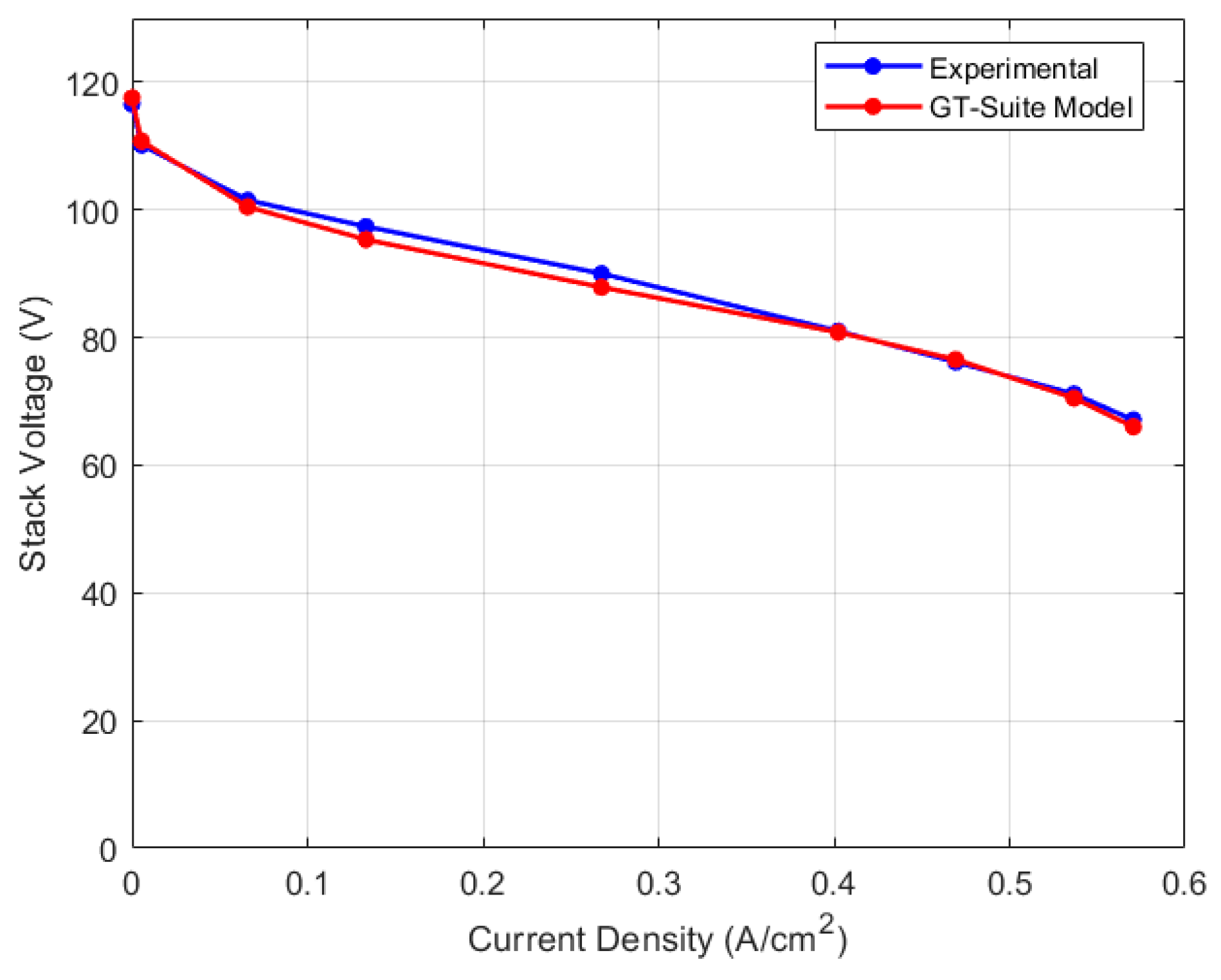
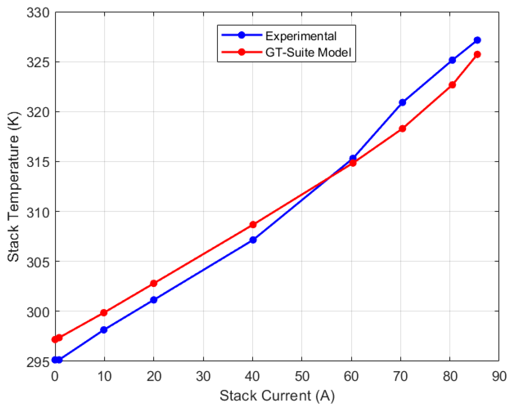
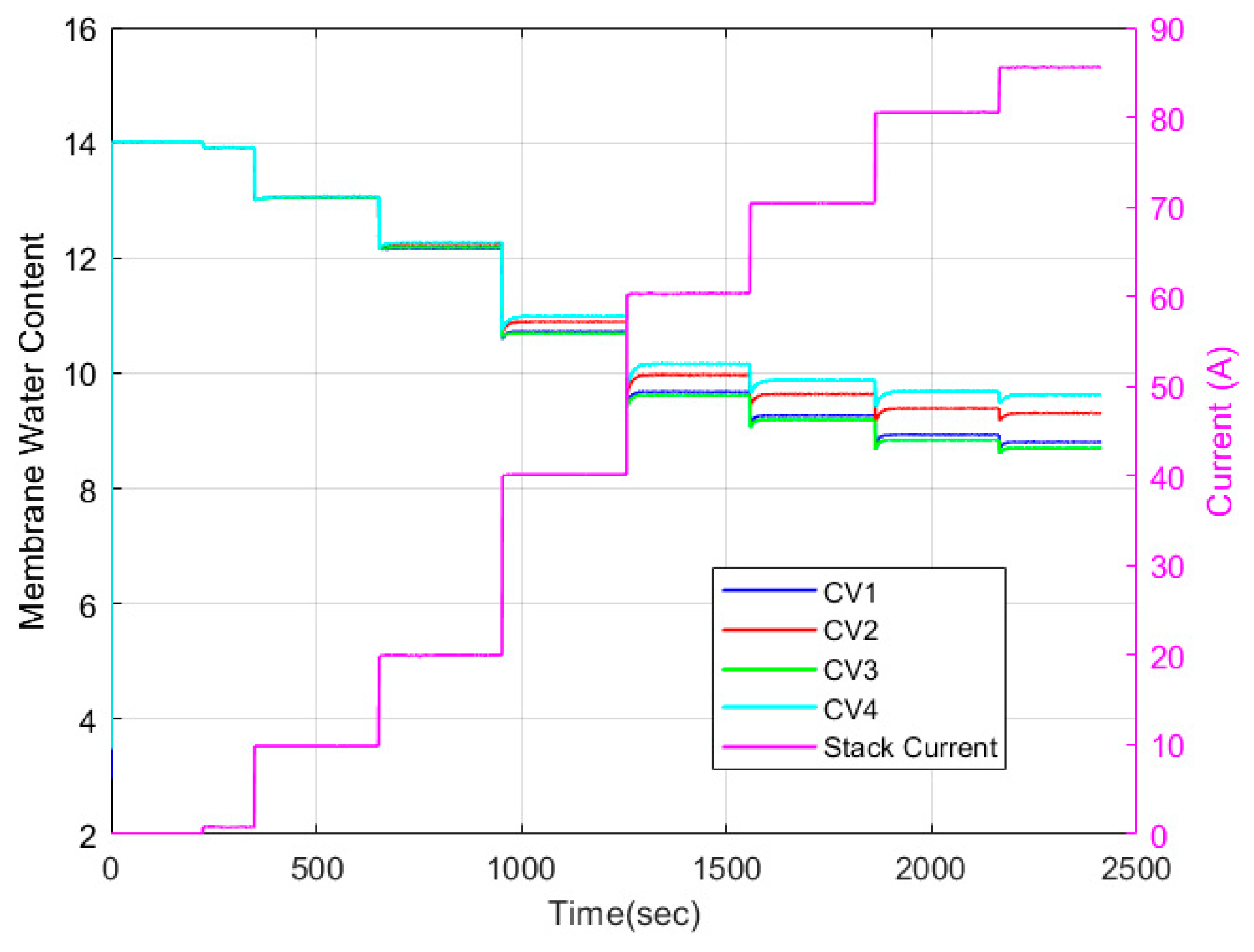
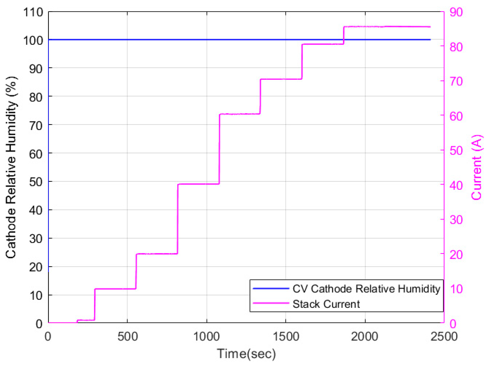
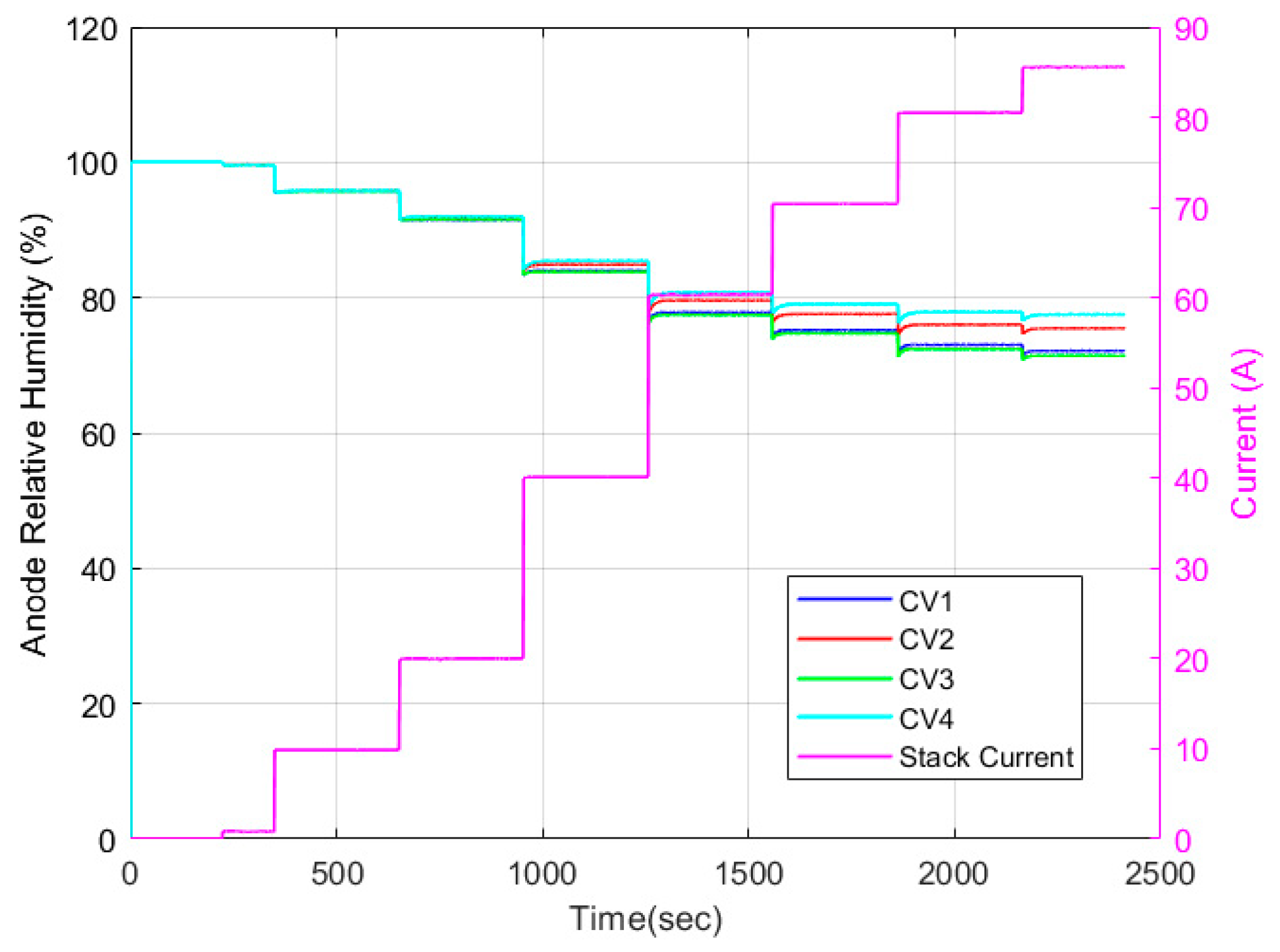
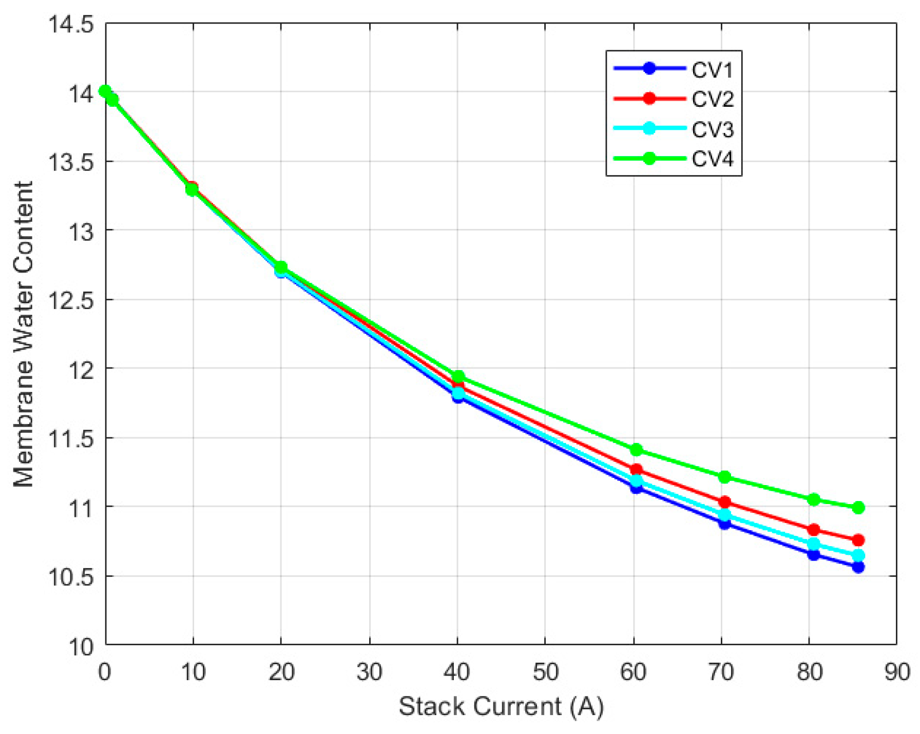
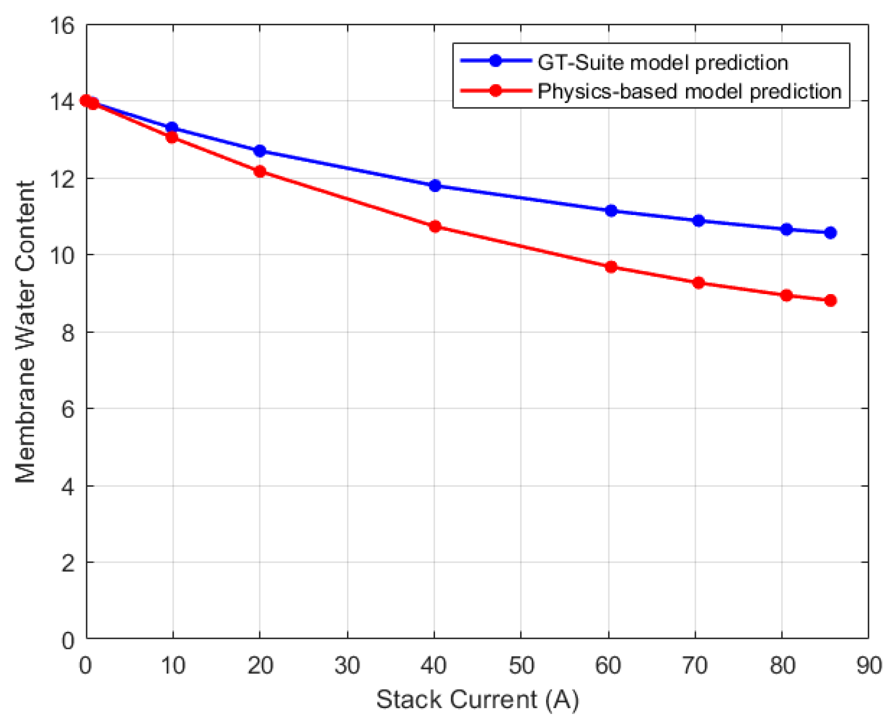
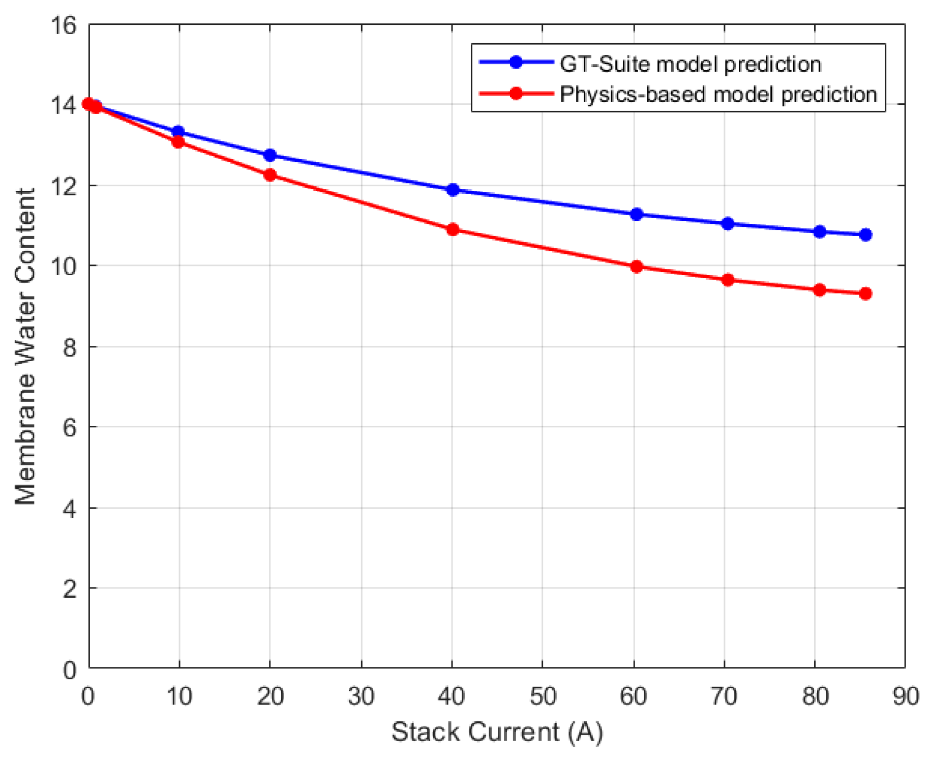
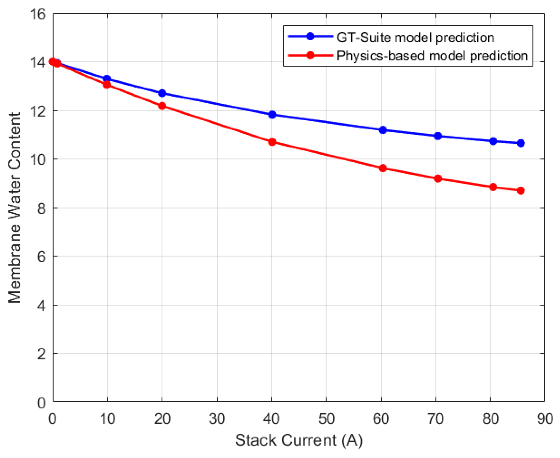
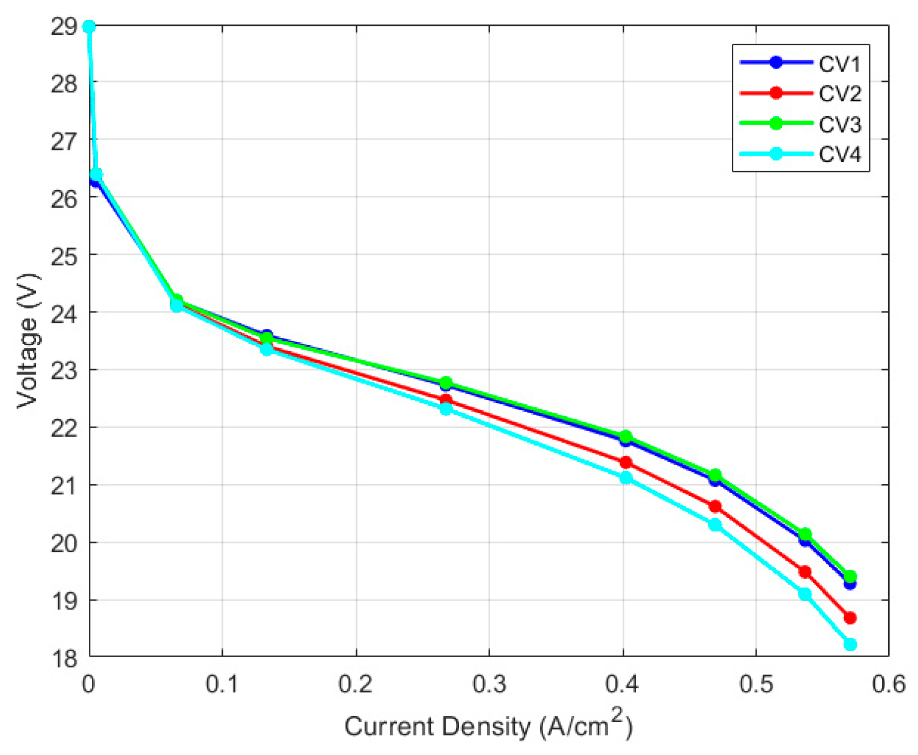
5.2. Discretized Model

While the lumped model captures the overall stack behavior, variations are present internally. The steady state experimental results of the temperature recorded by the four thermocouples are illustrated in Figure 12. As depicted in the figure, for low current regions (0 A–20 A), the temperature recorded by the thermocouples is comparable with a variation within 2 K. As the current increases, the temperature variation becomes more pronounced due to higher electrochemical reaction kinetics. Particularly at 85 A current, there is a maximum temperature variation of 10 K recorded. Notably, the left thermocouple (which is farthest from the direction of airflow) recorded the highest temperature for the medium to high current regions. This may be due to reduced cooling efficiency as a result of the location of the thermocouple. Interestingly, the mid-left thermocouple (just before the left thermocouple) recorded the lowest temperature at the higher current region. This suggests that the airflow may be directed in such a manner that it promotes effective cooling in this region.

The discretized model was validated using the experimental thermocouple measurements. For the discretized model, the temperature in CV1 corresponds to the right thermocouple reading, in CV2 it is the mid-right, in CV3 it is the mid-left, and in CV4 it is the left thermocouple. Figure 13, Figure 14, Figure 15 and Figure 16 display the thermocouple calibration results for each of the four thermocouples. The maximum relative error for each case is shown in

Table 3. Maximum relative error for discretized thermal model.

Thermocouple/CV	Max. Relative Error
	Physics-Based	GT-Suite
Right/CV1	0.92%	0.95%
Mid-right/CV2	1.08%	0.68%
Mid-left/CV3	0.89%	1.00%
Left/CV4	1.06%	0.75%

.

The membrane water content dynamics for each CV are shown in Figure 17. It is evident that the membrane water content varies along the stack. These variations are most noticeable in the medium to high current regions (40 A to 85 A) where there is increased water activity. Notably, the trends of the temperature variation results and the variation in membrane water content were the same. The CV with the highest temperature also had the highest water content. To gain a better understanding of the membrane water activity, the relative humidity dynamics occurring along the cathode and anode channels must be highlighted. The relative humidity dynamics in the cathode and anode channels are shown in Figure 18 and Figure 19, respectively. As can be seen, the cathode channel remained constant at 100% relative humidity for all CVs at all current cases. Conversely, the anode relative humidity varied along each CV. Hence, it is evident that the observed variation in membrane water content stemmed solely from variations in relative humidity in the anode channel. This explains why some researchers opt to model the membrane water content as a function of simply the anode water content since it is a limiting factor in determining the membrane water content.

To validate the discretized water management model, the model’s steady state predictions were compared to the simulation results from the discretized GT-Suite model. Firstly, the GT-Suite model was calibrated and validated using the thermocouple readings and the calibration results are illustrated in Figure 20, Figure 21, Figure 22 and Figure 23. The maximum relative error for each case is shown in Table 3. Following the validation of the GT-Suite model’s temperature variations prediction, its membrane water content predictions were used to validate the membrane water content variation in the physics-based model.

The steady state variation in membrane water content in the GT-Suite model is shown in Figure 24. As can be seen, the trends of the physics-based and GT-Suite models are comparable. The variations in membrane water content are much more evident in the medium to high current regions. The highest water content was recorded in the CV with the highest temperature. In the GT-Suite model, however, CV3 has a higher membrane water content than CV1 despite having the lowest temperature. Nonetheless, the difference in membrane water content between CV1 and CV3 for both the physics-based and GT-Suite models is only about 3%. A comparison of the steady state result of the physics-based model to the GT-Suite simulation results for each CV is shown in Figure 25, Figure 26, Figure 27 and Figure 28. For each CV, the trend of membrane water content prediction is the same.

Table 4. RMSE results for membrane water content comparison.

Control Volume (CV)	RMSE
CV1	1.17
CV2	1.00
CV3	1.27
CV4	0.95

shows the RMSE values between the models’ predictions. The physics-based model’s ability to predict the distribution of membrane water content in the stack is demonstrated by the RMSE, which was within 1.5 membrane water content for all cases.

As shown in Figure 29, temperature variation and its ensuing variation in membrane water content resulted in variation in voltage output along the stack. As can be observed, at low current density, the voltage output for each CV is identical, with an open circuit voltage of 29 V recorded by all four control volumes, but as the current density increases, the voltage output varies more noticeably. Particularly, CV4 recorded the lowest voltage output, while CV3 and CV1 recorded the highest voltage, with CV3 slightly exceeding CV1 in voltage. As determined from the thermal and water management physics-based models, CV3 had the lowest stack temperature and water content followed by CV1 while CV4 recorded the highest stack temperature and the highest water content. One possible explanation for CV3 and CV1’s enhanced performance could be due to the improved cooling system in these regions which resulted in the lower stack temperatures. Better cooling implies a higher air flow rate, which increases oxygen availability and, in turn, increases performance. It is, however, well documented that lower membrane water content leads to higher ohmic overvoltage in a PEM fuel cell stack. As a result, the reason for this performance gain is that the increased ohmic resistance is less than the enhanced performance brought about by oxygen availability.

6. Conclusions and Future Work

A reduced-order control-oriented physics-based model for predicting variation in membrane water content of an open-cathode PEM fuel cell was developed in this study. The water management model was validated by comparing its prediction to GT-Suite simulation results, and RMSE was found to be within 1.5 membrane water content for all cases. The results indicate that the water content of the PEM fuel cell membrane varies along the fuel cell stack. Variations abound, particularly in medium to high current density regions where there is significant water activity. The variations in the membrane water content coupled with the temperature variations lead to variations in the voltage output along the stack. Controlling these variations is, therefore, critical, especially during transients. The developed model thereby presents a computationally inexpensive means for the prediction and subsequent control of membrane water content variations. Compared to the lumped physics-based model which took ~12 s to simulate about 40 min of experimental data, the computational time for the 4-CV discretized model was ~80 s. Despite the increased computational time, it is still relatively low for control. In contrast, the lumped GT-Suite model took ~240 s to compute, which is almost 20 times slower than the lumped physics-based model. The computational time for the discretized GT-Suite model was ~600 s, which is about 7.5 times slower than the discretized physics-based model. The physics-based model is, however, limited to only vapor flow in the channels and cannot predict liquid water formation, which is important to prevent water flooding. Better prediction accuracy can be attained by incorporating a two-phase flow into the model to account for liquid water transport.

Future research will include experimentally validating the water management model to improve the model’s accuracy and reliability by aligning its predictions with real-world observations. In addition, the model will be improved to include liquid water effects to predict flooding conditions, particularly in the cathode channel.

References

1. Tellez-Cruz, M.M.; Escorihuela, J.; Solorza-Feria, O.; Compañ, V. Proton exchange membrane fuel cells (Pemfcs): Advances and challenges. Polymers 2021, 13, 3064. [Google Scholar] [CrossRef]
2. Zeng, T.; Zhang, C.; Huang, Z.; Li, M.; Chan, S.H.; Li, Q.; Wu, X. Experimental investigation on the mechanism of variable fan speed control in Open cathode PEM fuel cell. Int. J. Hydrogen Energy 2019, 44, 24017–24027. [Google Scholar] [CrossRef]
3. Morner, S.O.; Klein, S.A. Experimental evaluation of the dynamic behavior of an air-breathing fuel cell stack. J. Sol. Energy Eng. Trans. ASME 2001, 123, 225–253. [Google Scholar] [CrossRef]
4. Jeon, D.; Nam, K.; Man, S.; Hyun, J. The effect of relative humidity of the cathode on the performance and the uniformity of PEM fuel cells. Int. J. Hydrogen Energy 2011, 36, 12499–12511. [Google Scholar] [CrossRef]
5. Chen, Z.; Ingham, D.; Ismail, M.; Ma, L.; Hughes, K.J.; Pourkashanian, M. Effects of hydrogen relative humidity on the performance of an air-breathing PEM fuel cell: A numerical study. Int. J. Numer. Methods Heat Fluid Flow 2020, 30, 2077–2097. [Google Scholar] [CrossRef]
6. Ozen, D.; Timurkutluk, B.; Altinisik, K. Effects of operation temperature and reactant gas humidity levels on performance of PEM fuel cells. Renew. Sustain. Energy Rev. 2016, 59, 1298–1306. [Google Scholar] [CrossRef]
7. Watanabe, M.; Igarashi, H.; Uchida, H.; Hirasawa, J. Experimental analysis of water behavior in Nafion electrolyte under fuel cell operation. J. Electroanal. Chem. 1995, 399, 239–241. [Google Scholar] [CrossRef]
8. Zhang, Z.; Martin, J.; Wu, J.; Wang, H.; Promislow, K.; Balcom, B.J. Magnetic Resonance Imaging of Water Content across the Nafion Membrane in an Operational PEM Fuel Cell. J. Magn. Reson. 2005, 193, 259–266. [Google Scholar] [CrossRef] [PubMed]
9. Zhang, G.; Jiao, K. Three-dimensional multi-phase simulation of PEMFC at high current density utilizing Eulerian-Eulerian model and two-fluid model. Energy Convers. Manag. 2018, 176, 409–421. [Google Scholar] [CrossRef]
10. Dutta, S.; Shimpalee, S.; Van Zee, J.W. Numerical prediction of mass-exchange between cathode and anode channels in a PEM fuel cell. Int. J. Heat Mass Transf. 2001, 44, 2029–2042. [Google Scholar] [CrossRef]
11. Sagar, A.; Chugh, S.; Sonkar, K.; Sharma, A.; Kjeang, E. A computational analysis on the operational behaviour of open-cathode polymer electrolyte membrane fuel cells. Int. J. Hydrogen Energy 2020, 45, 34125–34138. [Google Scholar] [CrossRef]
12. Pukrushpan, J.T.; Peng, H.; Stefanopoulou, A.G. Control-oriented modeling and analysis for automotive fuel cell systems. J. Dyn. Syst. Meas. Control Trans. ASME 2004, 126, 14–25. [Google Scholar] [CrossRef]
13. Meyer, R.T.; Yao, B. Modeling and Simulation of a Modern Pem Fuel Cell System. In Proceedings of the ASME 2006 4th International Conference on Fuel Cell Science, Engineering and Technology, Irvine, CA, USA, 19–21 June 2006; pp. 133–150. [Google Scholar]
14. Chen, X.; Xu, J.; Fang, Y.; Li, W.; Ding, Y.; Wan, Z.; Wang, X.; Tu, Z. Temperature and humidity management of PEM fuel cell power system using multi-input and multi-output fuzzy method. Appl. Therm. Eng. 2022, 203, 117865. [Google Scholar] [CrossRef]
15. Chen, X.; Xu, J.; Liu, Q.; Chen, Y.; Wang, X.; Li, W.; Ding, Y.; Wan, Z. Active disturbance rejection control strategy applied to cathode humidity control in PEMFC system. Energy Convers. Manag. 2020, 224, 113389. [Google Scholar] [CrossRef]
16. Chen, F.; Zhang, L.; Jiao, J. Modelling of humidity dynamics for open-cathode proton exchange membrane fuel cell. World Electr. Veh. J. 2021, 12, 106. [Google Scholar] [CrossRef]
17. Headley, A.; Yu, V.; Borduin, R.; Chen, D.; Li, W. Development and Experimental Validation of a Physics-Based PEM Fuel Cell Model for Cathode Humidity Control Design. IEEE/ASME Trans. Mechatron. 2016, 21, 1775–1782. [Google Scholar] [CrossRef]
18. Nguyen, T.V.; White, R.E. A Water and Heat Management Model for Proton-Exchange-Membrane Fuel Cells. J. Electrochem. Soc. 1993, 140, 2178–2186. [Google Scholar] [CrossRef]
19. O’hayre, R.; Cha, S.-W.; Colella, W.; Prinz, F.B. Fuel Cell Fundamentals; John Wiley & Sons: Hoboken, NJ, USA, 2016. [Google Scholar]
20. Wang, Y.; Yu, D.; Chen, S.; Kim, Y. Robust DC/DC converter control for polymer electrolyte membrane fuel cell application. J. Power Sources 2014, 261, 292–305. [Google Scholar] [CrossRef]
21. Huo, D.; Hall, C.M. Data-driven prediction of temperature variations in an open cathode proton exchange membrane fuel cell stack using Koopman operator. Energy AI 2023, 14, 100289. [Google Scholar] [CrossRef]
22. Ishaku, J.; Lotfi, N.; Zomorodi, H.; Landers, R.G. Control-oriented modeling for open-cathode fuel cell systems. In Proceedings of the American Control Conference, Portland, OR, USA, 4–6 June 2014; pp. 268–273. [Google Scholar]
23. Karnik, A.Y.; Stefanopoulou, A.G.; Sun, J. Water equilibria and management using a two-volume model of a polymer electrolyte fuel cell. J. Power Sources 2007, 164, 590–605. [Google Scholar] [CrossRef]
24. Pukrushpan, J.T.; Stefanopoulou, A.G.; Peng, H. Modeling and control for PEM fuel cell stack system. Proc. Am. Control Conf. 2002, 4, 3117–3122. [Google Scholar]
25. Springer, T.E.; Zawodzinski, T.A.; Gottesfeld, S. Polymer electrolyte fuel cell model. J. Electrochem. Soc. 1991, 138, 2334–2342. [Google Scholar] [CrossRef]
26. Karthik, M.; Vijayachitra, S. An integrated exploration of thermal and water management dynamics on the performance of a stand-alone 5-kW Ballard fuel-cell system for its scale-up design. Proc. Inst. Mech. Eng. Part A J. Power Energy 2014, 228, 836–852. [Google Scholar] [CrossRef]
27. Zhang, Y.; Zhou, B. Modeling and control of a portable proton exchange membrane fuel cell-battery power system. J. Power Sources 2011, 196, 8413–8423. [Google Scholar] [CrossRef]
28. Falcão, D.S.; Pinho, C.; Pinto, A.M.F.R. Water management in PEMFC: 1-D model simulations. Cienc. e Tecnol. Dos Mater. 2016, 28, 81–87. [Google Scholar] [CrossRef]
Figure 1. Experimental setup.
Energies 17 00831 g001
Figure 2. Thermocouple layout for fuel cell stack.
Energies 17 00831 g002
Figure 3. Block diagram of physics-based model.
Energies 17 00831 g003
Figure 4. Block diagram of water management model.
Energies 17 00831 g004
Figure 5. Calibration results for stack voltage physics-based model.
Energies 17 00831 g005
Figure 6. Calibration results for lumped thermal physics-based model.
Energies 17 00831 g006
Figure 7. Calibration results for GT-Suite stack voltage model.
Energies 17 00831 g007
Figure 8. Calibration results for GT-Suite thermal model.
Energies 17 00831 g008
Figure 9. Comparison results for membrane water content.
Energies 17 00831 g009
Figure 10. Membrane water content dynamics for lumped physics-based model.
Energies 17 00831 g010
Figure 11. Relative humidity dynamics in the anode and cathode channels for lumped physics-based model.
Energies 17 00831 g011
Figure 12. Steady state temperature thermocouple data.
Energies 17 00831 g012
Figure 13. Right (CV1) thermocouple calibration results.
Energies 17 00831 g013
Figure 14. Mid-Right (CV2) thermocouple calibration results.
Energies 17 00831 g014
Figure 15. Mid-Left (CV3) thermocouple calibration results.
Energies 17 00831 g015
Figure 16. Left (CV4) thermocouple calibration results.
Energies 17 00831 g016
Figure 17. Membrane water content dynamics for discretized physics-based model.
Energies 17 00831 g017
Figure 18. Constant cathode relative humidity dynamics for all CVs of discretized physics-based model.
Energies 17 00831 g018
Figure 19. Anode relative humidity dynamics for discretized physics-based model.
Energies 17 00831 g019
Figure 20. Right (CV1) thermocouple GT-Suite calibration results.
Energies 17 00831 g020
Figure 21. Mid-Right (CV2) thermocouple GT-Suite calibration results.
Energies 17 00831 g021
Figure 22. Mid-Left (CV3) thermocouple GT-Suite calibration results.
Energies 17 00831 g022
Figure 23. Left thermocouple (CV4) GT-Suite calibration results.
Energies 17 00831 g023
Figure 24. Steady state membrane water content variation in GT-Suite model.
Energies 17 00831 g024
Figure 25. Steady state comparison of membrane water content for CV1.
Energies 17 00831 g025
Figure 26. Steady state comparison of membrane water content for CV2.
Energies 17 00831 g026
Figure 27. Steady state comparison of membrane water content for CV3.
Energies 17 00831 g027
Figure 28. Steady state comparison of membrane water content for CV4.
Energies 17 00831 g028
Figure 29. Voltage variation along stack for physics-based model.
Energies 17 00831 g029