Abstract
External disturbances, uncertainties, and nonlinear behavior are problems that are commonly encountered by control system designers. In order to save on energy and materials, mechanical structures have become lighter and more flexible, which only exacerbates the control problem. To resolve this issue, robust and adaptive control strategies have been proposed and have recently gained a lot of interest in modern scientific literature. This article proposes a combination of both approaches: a sliding mode—radial basis function neural network controller applied to an electrical drive with a sophisticated mechanical structure. The proposed sliding surface provides robustness against parameter uncertainties, while the neural network adjusts itself to the current state of the drive and mitigates the oscillations resulting from the elastic connection with the load machine. This article proves the stability of the proposed control algorithm in the sense of Lyapunov, provides an in-depth numerical analysis, and compares those results with the experimental tests. The algorithm was implemented in a 1103 dSPACE fast-prototyping card and was used to control a 0.5 kW DC motor connected to the load machine by a long (thin) steel shaft.
1. Introduction
Nowadays, constant growth of basic requirements in the field of modern industry can be observed. Almost every aspect of novel solutions needs to be more efficient, versatile, easy to apply, and economical, both during development and maintenance. One of the basic demands of modern industry is to make applied solutions more cost-effective while increasing the execution capabilities of the implemented algorithm. The described trend is particularly visible in the field of electric drives. Currently, the observed transformation of global transportation (e.g., hybrid and modern electric trains, electric cars) leads to a gradual increase in energy consumption, both globally and locally in individual households [1]. Conventional control systems are proven to be efficient enough to handle typical applications of electric drives, e.g., cooling fans, air conditioners, etc. However, consistent extension of possible electric drive applications, such as wind turbines [2,3], robotic manipulators [4,5,6,7], and exoskeletons [8,9], often implicates the necessity of handling a sophisticated and complex mechanical structure. One of the possible reasons for potential problems is related to lighter mechanical construction, which gives the structure more flexibility [10]. From the point of view of the control structure, it may cause some stability issues [11]. Lighter construction changes the mechanical time constants of the system, which may provoke more oscillations and reliability problems [12]. Moreover, due to a huge variety of possible applications of electric drive systems, a possible change in the external environment of the drive needs to be taken into consideration as well [13]. A massive payload carried by the robot driven by electric motors combined with, e.g., a strong wind, may cause a significant reduction in accuracy or a different path trajectory. In terms of space robots, a common problem is related to a change of static and dynamic friction, which can also create additional uncertainty and make correct identification of the plant unfeasible [14]. Furthermore, limited motor torque and a variety of payloads that can be carried by the electric drive-powered system is undeniably a huge concern, which forces the need to make modern control systems even more insensitive to any kind of disturbances [15]. Additionally, with all the instantiated issues, problems typical for electric motor control, such as actuator saturation and faults need to be taken into account [16,17]. The control signal established by the controller should remain within certain limits that do not exceed the actuator’s movement capabilities. Otherwise, discrepancies may occur in the control structure and the device may stop responding accordingly to the given control input. In order to ensure sufficient dynamics and fulfill all initial requirements of the drive, robust control systems are commonly used.
Robust control structures are a common approach in the field of controlling a plant with variable or floating parameters. Its main idea is focused on tacking the plant parameters uncertainty in a specific way, allowing the closed-loop control system to have eligible dynamics. The key feature of the robust control system is the constancy of its parameters. In other words, the control system stays insusceptible despite the plant parameters being changed in a specific, limited range, within which the response of the system is approved by the user. proportional-integral-derivative (PID) [18], H∞ [19], sliding mode [20], and fuzzy logic controllers [21,22,23] are typical robust control solutions used in modern industry.
Fuzzy logic is considered to be one of the staple components in the list of modern robust controllers. Its main idea is to show and interpret an input signal in the form of ambiguous, linguistic variables. This approach allows the user to simplify the whole design process of non-obvious, unusual, and non-linear systems, which would be difficult to describe with mathematical equations [24]. By doing so, fuzzy logic solves the problem of needing to define phenomena in order to create a proper control system. On the other hand, defining the rule base and assigning an appropriate set of initial weight parameters of a fuzzy logic controller requires a lot of human experience or forces the necessity of using advanced optimization algorithms (presently meta-heuristic algorithms are commonly applied in the design of control systems and electric machines) [25,26]. A typical fuzzy logic controller consists of three main parts. The first one is responsible for converting the input data into linguistic variables. Then, the inference process is initiated, which leads to determining the final decision. The last stage of data processing inside of a fuzzy logic controller is changing the final linguistic value into a numerical value [27]. The described solution is capable of working on not fully identified plants and cooperating with the rest of the control system, e.g., the PI current controller. They are used in applications with ambiguous or variable mechanical parameters, e.g., cruise control in cars, where the mechanical time constant of the plant is changed alongside gear changes.
One of the most popular approaches to robust control is sliding mode control. It is based on the mathematical model of the plant [28,29,30]. The internal structure of the controller stays unchanged and is insusceptible to plant parameter change in a specified range. The main idea of the sliding mode control structure is to switch the control signal between positive and negative values in a way that makes the system follow the reference trajectory, described by a switching surface. The desired dynamics of the system can be described in the design process of the controller by defining a proper equation of the switching surface [31,32]. Because of the fact that the control system switches the steering signal every time it crosses the switching line, the control law is realized by a signum function. The goal of the mentioned control structure is to bring the phase plane trajectory to zero. Sliding mode control features excellent dynamics and low vulnerability to external disturbances and parameter changes. Because of the fact that sliding mode control does not contain the integrator block, it is possible for a steady-state error to occur [33]. Moreover, in the case of using the sliding mode control, the appearance of chattering is inseparable, which is one of the biggest inconveniences of the described structure.
However, a hypothetical change of plant parameters may involve a bigger difference than assumed, which may not be corrigible by the control system. Robust controllers are considered a good solution to compensate for inaccuracy committed during the design process of the controller. That is the reason why adaptive control systems have been introduced. Adaptive systems are designed specifically to deal with possible plant electromagnetic or mechanical time-constant change. The main feature of adaptive systems is the fact that both the parameters and structure of the controller can be changed on the fly.
The first type of adjustable control system is described as gain scheduling. The structure of the controller in general is constant. The whole system is equipped with a decision making unit with implemented information about possible signal disturbances which may occur unexpectedly. When this happens, the parameters of the controller are changed according to the information contained in a look-up table. The whole process is based on what is called a “process variable”, which stimulates the decision making unit to change specific parameters in a particular time window. However, the lack of feedback from the plant is a big inconvenience of the described structure, which makes it usable only in a predefined range of parameters.
The Model Reference Adaptive System (MRAS) is considered to be one of the most common solutions of all adaptive approaches [34]. Its main idea is based on calculating the adaptation error value. That signal is described as the difference between the actual plant output and its reference model [35,36]. The moment any error appears, the algorithm forces the instant change of the controller parameters. The described solution deals perfectly with inconsistent plant parameters. A significant advantage of this system is the possibility of creating the desired dynamics of the system by defining a proper transfer function of the reference model. However, despite its excellent response and adaptation abilities, MRAS is not efficient when it comes to constant value regulation, which may be problematic in many areas. It works best when the reference signal changes periodically.
Today, in order to satisfy the initial demand of the market and applications, sophisticated machines and appliances require basic robustness combined with adaption capabilities. That forces the industry to reach novel control systems based on neural models. Neural networks are becoming a common tool used in today’s control theory. Apparently, neural networks are a widespread solution used in the field of electric drives as well [37,38,39]. Considering the fact that a novel electric drive system demands a quick response for each disturbance or possible change of the parameters, it is crucial to match the used model to the current application. Wide, deep-learning-based models may not be the best solution in terms of dynamic speed control with adaptation capabilities [40]. The offline training method excludes these networks from use in control systems due to their lack of adaptive properties. Nonetheless, there are many different solutions that suit the adaptive control idea adequately. The radial basis function neural network (RBFNN) is considered to be one of the answers for the described task. Those networks are widely implemented in many fields of science [41,42,43,44,45,46]. Because of their simplicity, they are often used in non-linear systems, solving mathematical equations, or estimating state variables of particular systems. RBFNN is a simple neural network with a single hidden layer of neurons. Each of them uses an exponential activation function. The low complexity of radial basis function neural networks combined with their adaptation abilities allows developers to use them as a closed-loop speed controller. Furthermore, RBFNN uses a simple training method, which operates by minimizing the cost function based on the input signal error. This allows it to be immediately applied to control systems, as it does not require complex, long-standing offline training. Furthermore, using online training allows the network to adjust its weight coefficients on the fly based on the analyzed input signal.
Multi-mass systems are a stellar example of a plant that incorporates the above-mentioned problems: possible variance in plant parameters, complex and non-linear behavior, as well as the presence of external disturbances [47]. In appliances driven by electric motors, PI controllers are usually implemented to regulate the speed of the machine [48]. However, when the machine has a complex mechanism, this type of control is not adequate [49]. This control structure does not provide enough information about the state of the drive to supply correct control signals. As a result, the response of the system can be characterized by substantial overshoots with no oscillation damping capabilities. One way to tackle this issue is to provide additional feedback to the control structure [50]. Information about other state variables can enable the algorithm to minimize the discrepancy between the speed of the motor and the load machine. A special case of control strategy with feedback from variables other than the output of the system is referred to as state-feedback control with integral action. In this strategy, the basic principle is to make the control signal dependent on more than one variable, controlling not only the output variable but also allowing the movement of the plant to the desired state. Unfortunately, neither of those algorithms can withstand parametric changes in the plant, making their sensitivity the biggest issue. Therefore, some form of adaptation or robustness must be incorporated as an enhancement if those algorithms are to be selected.
Perpetual improvement of novel computational modules provides a huge range of new possibilities. Common access to powerful micro-controllers and modern digital signal processors incites scientists and engineers to develop more complex algorithms, which are specifically designed to solve advanced problems. Moreover, the current development of neural networks defines the modern approach to use a new variety of computational units in the form of FPGA modules. Besides the quality of control, the designers also must take programmable device resource utilization into account. The control algorithm usually is not the only implemented component. In some applications, diagnostic tools [51], estimation algorithms [52], and communication with other devices must be incorporated as well. Additionally, very often project funding limits must be considered, which sometimes makes it impossible to use state-of-the-art arithmetic units. Because of that, memory usage must be managed carefully.
In this article, a resource-friendly control algorithm enhanced by robust and adaptive properties—a sliding mode radial basis function neural network (SM-RBFNN) controller is proposed. Both of the components are not computationally heavy, as the sliding surface only requires the numerical calculation of the error derivative, and the selected topology of the RBFNN consists of just five neurons in the hidden layer. The operation of this strategy will be verified with a two-mass system selected as the controlled plant. Combination of RBFNNs and SMC has already been investigated in the literature [53,54]. However, usually, the RBFNN is used purely as an adaptation tool for the sliding surface gains. The novelty, and the main contribution provided by this paper, is an investigation of the possible use of RBFNN as a substitute for sign function, which means that it is directly responsible for generating the control signal. The motivation for this research emerges from the main drawback of the sign function—the chattering effect caused by its discontinuity. The RBFNN is expected to completely mitigate this problem. Moreover, due to the weights being adapted continuously, the elimination of steady-state error as well as the addition of adaptive properties are achieved.
This paper is organized as follows: In the next chapter, the mathematical description of all the components of the control structure is given. The stability of the system is also proven. Then, preliminary numerical studies are conducted to confirm the theoretical assumptions. Matlab/Simulink (ver. 2020b) environment is incorporated for this task. The influence of all the adjustable parameters of the algorithm is shown. The subsequent section presents the results obtained during the experimental verification. The laboratory workbench is comprised of two DC machines connected through a long, thin, steel shaft. The algorithm is implemented in a 1103 dSPACE fast prototyping device. In the final section, the results are discussed and this study’s most important findings are summarized.
2. The Proposed Sliding Mode Radial Basis Function Neural Network Controller for a Two-Mass System
2.1. Mathematical Model of the Considered Electric Drive Mechanical Structure
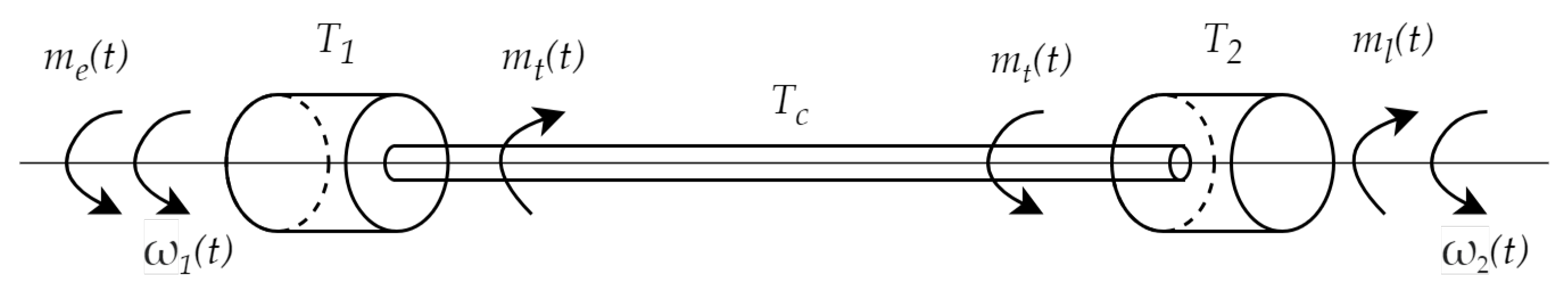
Numerous industrial applications are affected by elasticity in the connection between the driving machine and the effector. Two-mass structures are often selected as test plants for control system design purposes. The name refers to a structure of two masses conjoined by a flexible element. Each of the elements is characterized by its own inertia, which is recalculated into a time constant, which can be used with transfer functions in the Laplace domain or state-space equations. The mathematical description of a two-mass system’s behavior can be given with the following state-space equation [55]:
where —angular speed of the motor, —angular speed of the load machine, —torsional torque, —electromagnetic torque, —load torque (external disturbance), , , —mechanical time constants of the motor, load machine and shaft, respectively. From the effectiveness point of view, the most attention should be paid to how the load machine operates. However, from the control design perspective, information about the current state of the motor is equally as important. Therefore, the output of the system can be described as:
The equations can be visually interpreted by a diagram shown in Figure 1.
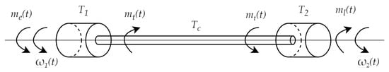
Figure 1.
Schematic interpretation of two-mass system described with Equation (1).
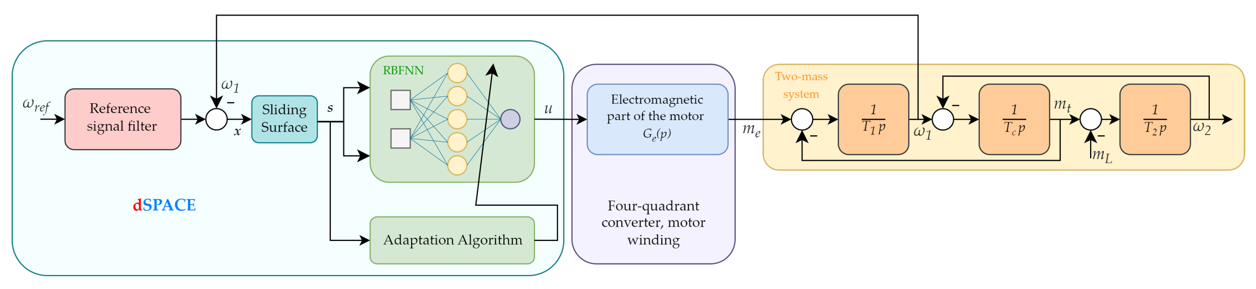
In its nature, the two-mass system’s state variables are dependent on each other. This level of sophistication creates a serious control problem that has become one of the leading research topics in scientific facilities around the globe. In order to conduct the required tests and simulations, the presented mechanical system can be also described in the form of transfer function blocks realized in the Laplace domain. The model of the whole control structure is shown in Figure 2.
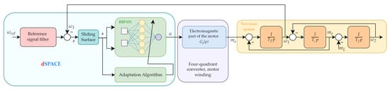
Figure 2.
The block diagram of proposed control system.
The part of the control system responsible for generating electromagnetic torque is described with the following equation:
where: —current control loop time constant, p—Laplace operator.
The detailed structure of the speed controller proposed in the described approach is presented in Section 2.3.
2.2. Principles of Operation of Radial Basis Function Neural Networks
Radial basis function neural networks are a subcategory of feed-forward neural networks. Their name is derived from the type of activation function used in the hidden layer neurons. There are several parameters that need to be selected before an RBFNN is fully established. First, an equation describing the radial basis function must be selected. The most common activation function that can be found in the literature is the Gaussian function. Conventionally, in the RBFNNs, there are always three layers, namely the input, the hidden, and the output layers. However, attempts are made to create multi-layer RBFNNs, which increase the network’s capability to accurately represent the input space [56]. The number of radial neurons then needs to be established. This task can be performed, e.g., through the use of clustering algorithms, such as Growing Neural Gas (GNG) [57] or Expectation Maximization (EM) [58] algorithms. The output of each of these neurons is dependent on two parameters: the Euclidean distance between the input variable and its center vector, and the width of the function. Finally, the values of the weighted connections between the hidden and output layers need to be established. The values can be calculated with gradient-based algorithms (such as gradient descent). For this purpose, a learning coefficient needs to be established and adjusted. Moreover, for online training (i.e., training performed simultaneously with the cooperating process) possible addition of momentum factor and careful selection of the initial weights may need to be considered if the training process begins to oscillate around the minimum of the cost function to facilitate the convergence process.
Activation level h of the i-th hidden layer neuron can be described with the following equation [59]:
where —input of the neural network, —neuron center vector, and —gaussian function width coefficient.
The output of the RBFNN can be then defined as [60]:
where —weight coefficient corresponding to the i-th neuron.
2.3. The Proposed Control Scheme—Sliding Mode-RBFNN Controller Applied to a Two-Mass System
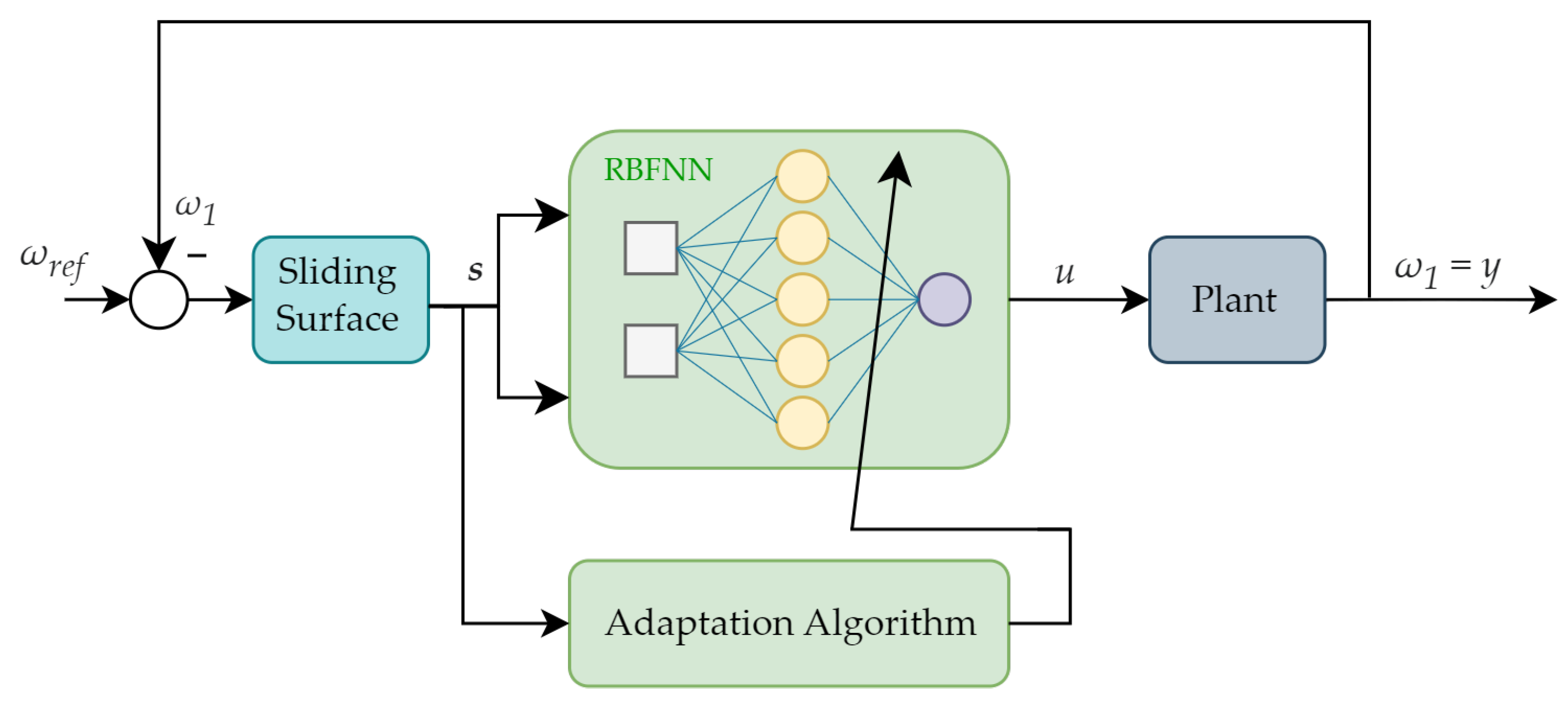
A typical sliding mode control uses a switching surface equation passed through an additional function. Its role is to execute the control law of the system. In the proposed algorithm, a novel approach in the field of electric drives has been proposed. The control law of the sliding surface is executed with the use of an RBFNN. The input signal for the network and the adaptation algorithm is constituted of the switching surface equation values [61]. Despite having typical sliding mode control robustness, the described solution offers additional adaptation capabilities. The description of the overall structure of the control system is based on the scheme shown in Figure 3. The proposed approach assumes a lack of information about the speed of the load machine. This leads to the conclusion that motor speed is the only state variable taken into consideration in the described control system. The speed of the load machine is examined in terms of appropriate work of the speed control loop but is not used in the main control process. Considering what is mentioned above, the further presented analysis omits the second motor speed and treats the speed of the motor as the plant output.
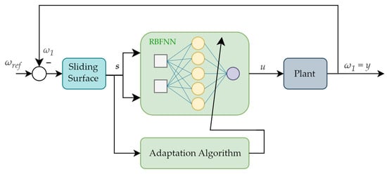
Figure 3.
The overall structure of the control system.
2.3.1. Theoretical Background of the Sliding Surface Design Process
The main goal of the sliding mode control algorithm is to obtain a quick, inertial response of the plant. That being said, the desired dynamics of the system can be obtained by defining an appropriate mathematical formula in the form of a first-order transfer function:
where: —demanded time constant of the plant, which enforces the slope of switching line.
The transfer function included in Equation (6) can be also described as a correlation between the output and the input of the system, which in our case can be substituted as follows:
which after conducting some transformation can lead to the expression:
Thus, considering the above-mentioned mathematical formula and switching to the time domain one can obtain the following formula:
which can be rewritten as:
Assuming that two state variables are defined, we can describe the system with the following state space equation. To simplify the notation time domain has been omitted:
which can be simplified to:
By differentiating (12) one can get:
Having summarized all of above considerations, demanded phase plane straight line equation can be described as follows:
The goal of the sliding mode controller is to minimize the value of the switching surface, which can be presented as:
which can be simplified to the following expression:
With respect to transformations presented above, a sliding surface equation can be written as:
which leads to final switching law equation:
2.3.2. Design Methodology of the Proposed SM-RBFNN Controller
Due to common uncertainties of sliding mode control (e.g., chattering, possible steady-state error), in this study the switching law function (sign) is substituted with an RBFNN. The overall structure of the proposed algorithm is presented in Figure 3.
Input of the RBFNN is defined as:
where s—sliding surface, —sampling period.
The sliding surface can be defined as follows:
where: —error derivative gain, .
Above formula leads to Equation (4) taking the following form:
Considering the overall structure of the control system (shown in Figure 3 and Equation (21)), the sliding surface can be described as follows:
Because of the fact that , Equation (23) can be also written as:
Finally, the control law can be described as the output of the Radial Basis Function Neural Network:
2.4. Adaptation Algorithm of the Proposed Control Structure
The adaptation algorithm refers to the change of weight coefficients of the radial basis function neural network. It is based on a gradient descent method. Its main idea is focused on minimizing the value of the cost function. In the described case, the cost function can be defined as:
The values of the variable parameters are modified according to the information about the derivative of the cost function with respect to the weights:
Applying the chain rule leads to the expression:
thus:
where: —plant derivative.
2.5. Stability Analysis
Stability analysis is one of the most critical aspects of the whole control system design process. In terms of non-linear plants, it is crucial to examine the stability both with global and local approaches. Lyapunov Stability Theory is one of the key findings in the field of stability analysis of non-linear systems. In the proposed survey, the convergence of the adaptation algorithm of the proposed SM-RBFNN controller is investigated as well. The core of the Lyapunov theory in general refers to the time-varying non-linear system stability. For the following system, it is demanded to define a Lyapunov candidate function ensuring the following condition is accomplished [62,63,64]:
Assuming that the value is positive, that leads to the conclusion that the system stays globally stable in the sense of Lyapunov when the following condition is fulfilled:
In the proposed approach the cost function was chosen as a Lyapunov candidate function:
Moreover, a value of weight coefficients in the following time moment can be described as:
Similar dependence can be applied to the value of switching surface in a particular time moment:
By elaborating further on Equations (34) and (35), the following expansions can be obtained [62]:
According to the Lyapunov theory, the system is stable when the following equation is ensured:
Thus, the combination of Equations (35)–(37) provides the following formula:
If the derivative of the Lyapunov function is limited to be negative, this ensures that the Lyapunov function only decreases and proves that the system is stable. Therefore, in order to accomplish that condition, the following condition must be fulfilled:
which can be re-written as:
After conducting a proper transformation of Equation (41), the final stability condition can be described as follows:
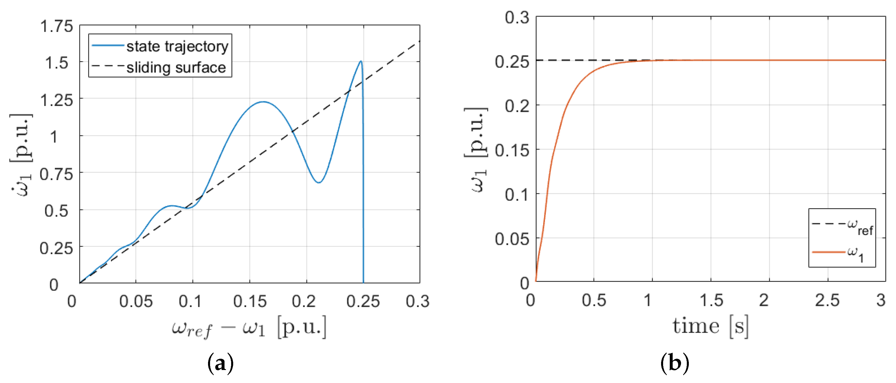
In order to confirm the propriety of the obtained stability condition, the value of the Lyapunov candidate function was numerically calculated. Its transient as a step reference signal response is presented in Figure 4.
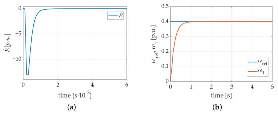
Figure 4.
Transient of proposed Lyapunov function: (a) derivative of the Lyapunov candidate function; (b) corresponding step response of the motor angular velocity.
3. Tests of the SM-RBFNN Controller Applied to the Drive with Elastic Shaft
Tests of the implemented structure are divided into two parts. The first one involves simulations conducted in a Matlab/Simulink environment. This stage refers to modeling a proper mechanical model, conducting initial tests of the structure, and adjusting the parameters of the control system and neural network. The second part contains the laboratory experiment. Its goal is to prove that the proposed solution fulfills all initial requirements.
Simulation Results
The simulation stage of the test was initiated by modeling the control system of the drive in a Matlab/Simulink environment. The simulation model was based on the scheme shown in Figure 2. The reference signal is realized in the form of an adjustable square wave with the following parameters:
- ,
- Hz,
where: —signal amplitude, f—signal frequency.
In order to keep all conducted tests objective, all initial parameters of the neural network were kept at the same level during the first attempts. The implemented vector of the neuron’s centers can be described as follows:
The applied vector of initial weight coefficients can be described as:
Additionally, the rest of the changeable parameters consist of the width of each neuron, momentum, and learning rates. Each of the mentioned parameters takes consecutive values:
- ,
- ,
- ,
where: —width of the Gaussian activation function, —momentum rate, —learning rate.
The additional load was initiated at s. The step assumed for numerical calculations was equal to ms.
At the beginning of the simulation tests stage, the sliding surface trajectory defined with Equation (24) was verified. The obtained results are presented in Figure 5.
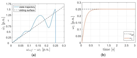
Figure 5.
Sliding surface tracking for the proposed control algorithm: (a) Response of the state trajectory; (b) corresponding step response of the load machine angular velocity.
In the designed control system, an additional reference signal filter was used. Due to the inertia of the electric motor, it is not capable of following a typical square wave with such a steep slope. The purpose of using a reference signal filter was to avoid the situation, where the adaptation algorithm would be stimulated without having a physical chance to compensate for the speed error that occurred. The applied filter can be described with the following transfer function:
where: —angular frequency, —damping coefficient, p—Laplace operator.
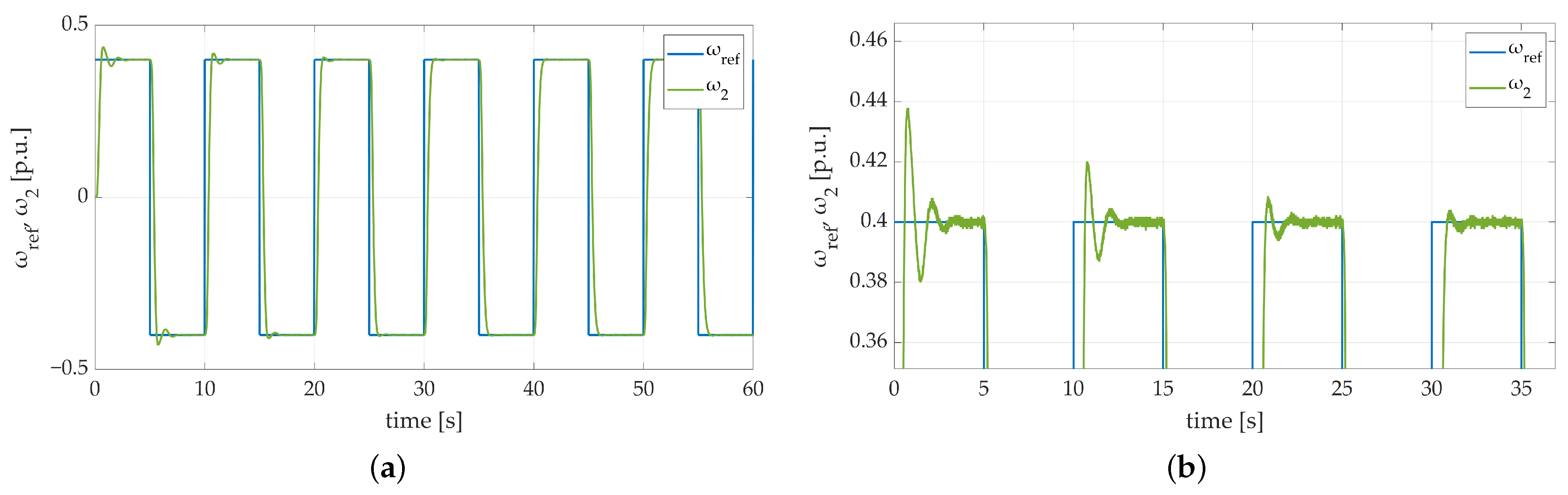
The first attempt of the tests was carried out to verify the correctness of the system behavior with default parameters taken into account. The achieved results are shown in Figure 6.
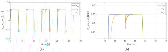
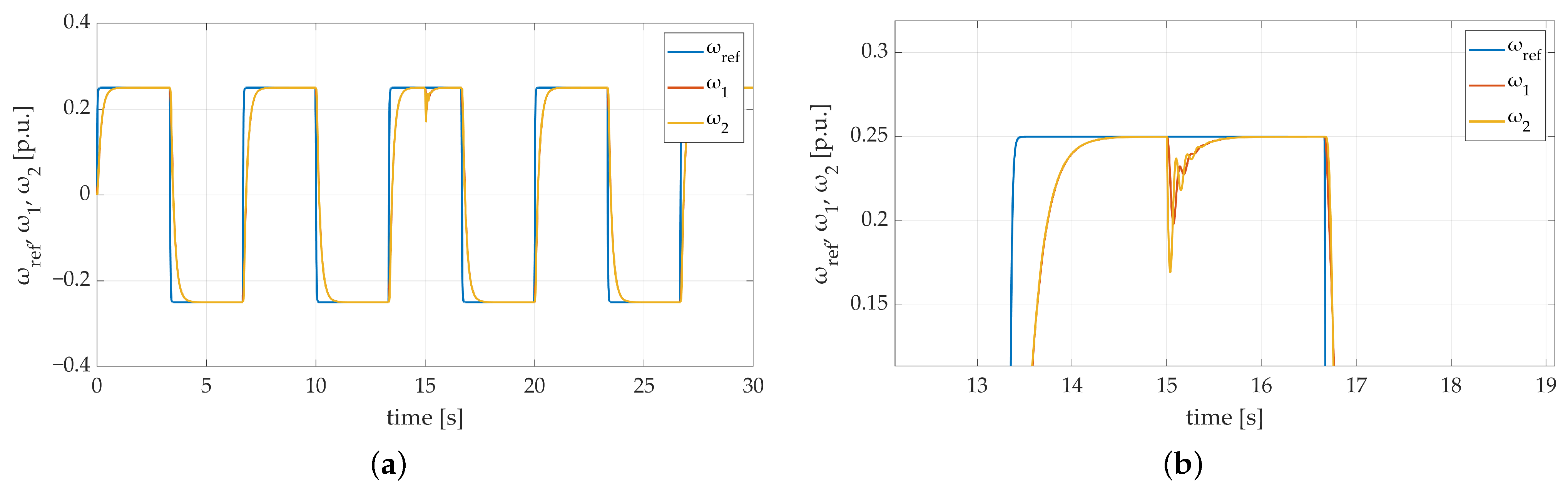
Figure 6.
Speed transients of the two-mass electric drive system with elastic shaft and SM-RBFNN controller: (a) a general overview of the simulation run; (b) a zoom-in showing the moment of attachment an additional load torque.
The general results of the presented attempt are shown in Figure 6a. It can be observed that both motor and load speed follow the reference trajectory. No overshoots are visible after each speed direction change. Furthermore, the steady-state error does not exist as well. The moment of attachment of the additional load torque is presented in Figure 6b. A small difference between particular speed values is visible. Considering the fact that the elastic shaft was used in the system, the mentioned speed difference is negligible. Speed error, which occurred during the additional load torque attachment, is taken down to zero instantly.
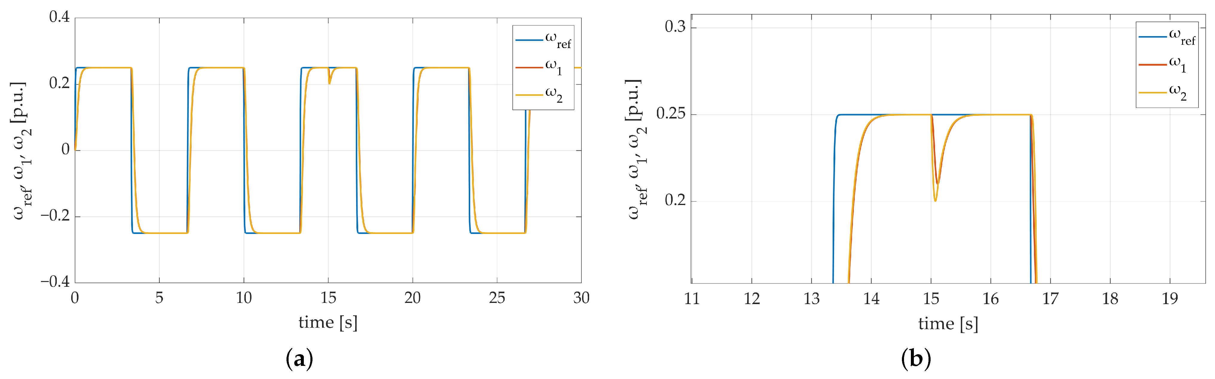
The next stage of simulation tests contained a significant increase in mechanical time constant value . In order to simulate an extreme situation, the mentioned parameter was increased 3 times. The obtained results are shown in Figure 7. The actual values of the motor and load speed directly follow the reference signal. There are no overshoots visible on the obtained transients. The dynamics are at the same level as they were during the first attempt with default parameters. The only noticeable difference can be seen in Figure 7b. After applying additional load torque both speed transients are brought back to the reference level more smoothly.
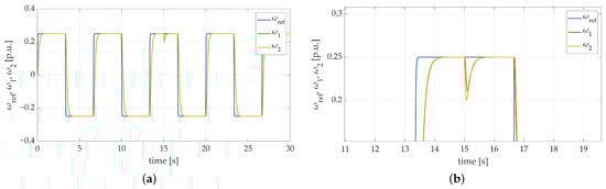
Figure 7.
Speed transients of the two-mass electric drive system with elastic shaft and SM-RBFNN controller with the time constant increased 3 times: (a) a general overview of the simulation run; (b) a zoom-in showing the moment of attachment of additional load torque.
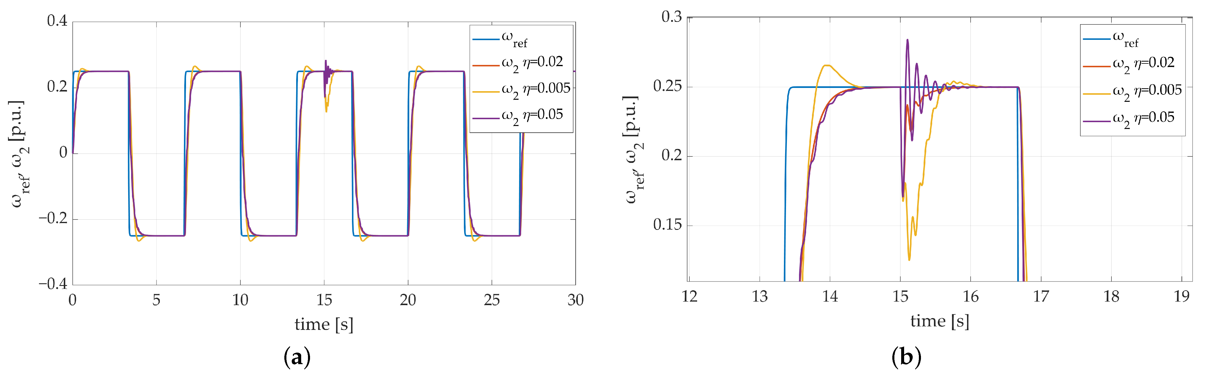
The idea of the third conducted test was to examine the influence of the learning rate change on the whole control system behavior. To do so, a first attempt at the third test included three learning rate values: , , . To emphasize the influence of the changed parameter and to increase the readability of the graph, load speed was taken into consideration only. The obtained results are shown in Figure 8. The difference in system behavior is significant. The influence of the learning rate value is particularly visible during additional load torque attachment. Not only does the higher value of the examined parameter have no positive impact on the system dynamics, but it also causes some unwanted oscillations. On the other hand, too small a value of the learning rate parameter may cause some overshoots to occur. Despite the plant response being different, it is brought to the reference speed trajectory after each return and the whole system remains stable in both cases.
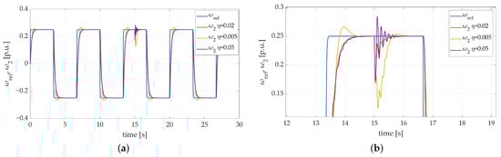
Figure 8.
Transients of the two-mass electric drive system with elastic shaft and SM-RBFNN controller with different learning rate values: (a) a general overview of the simulation run; (b) a zoom-in showing the moment of attachment of additional load torque.
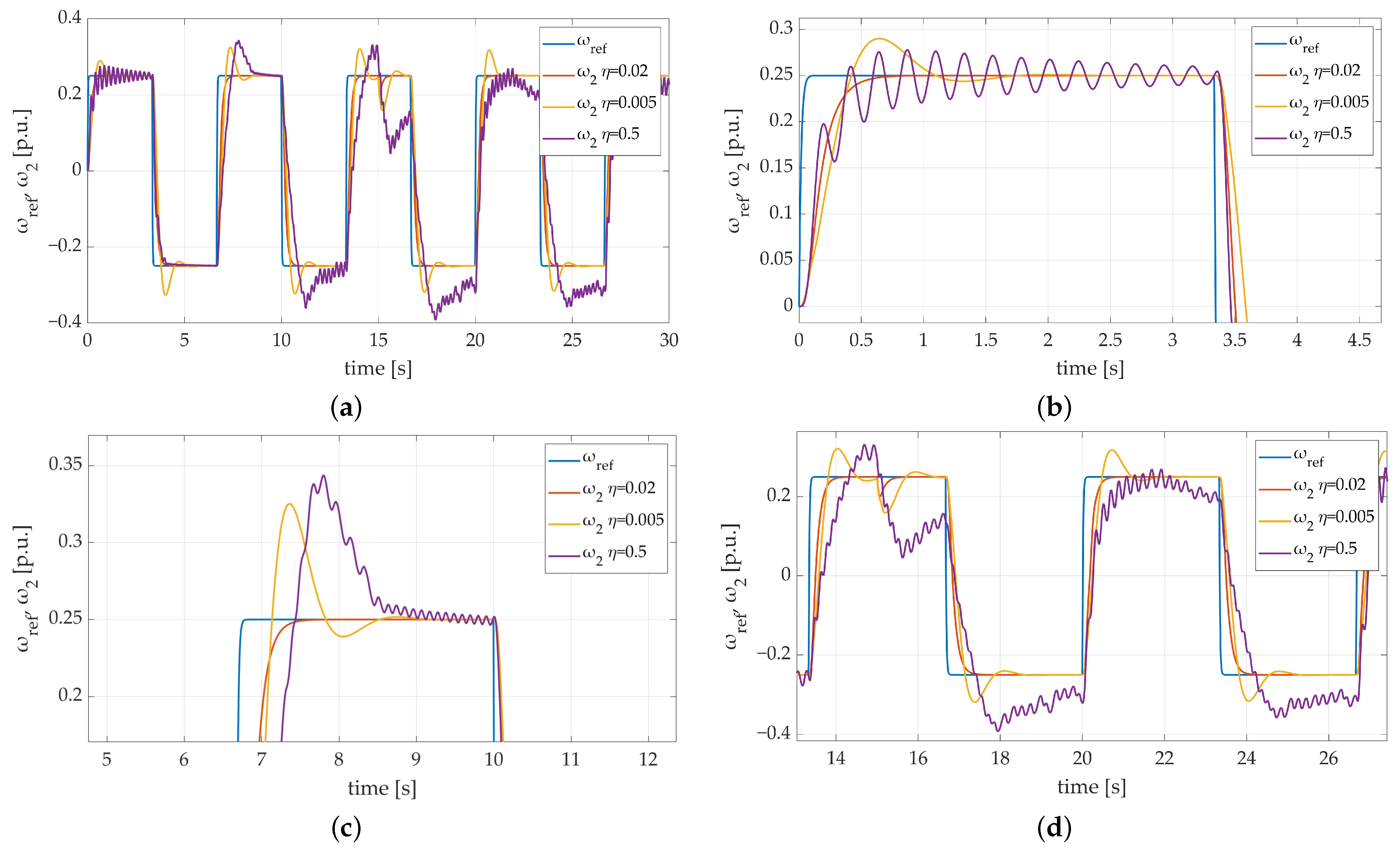
However, values tested in the previous attempt were not extremely different from the default parameter. In order to examine the behavior of the system in extreme conditions, an additional attempt was made. In this case, the value was examined. To make the conditions of the test even more extreme, the value of mechanical time constant was increased three times again. Speed transients presented in Figure 9 prove that it is required to find an optimal value of the learning rate parameter. An unlimited increase in the examined parameter may cause dangerous stability loss. Nonetheless, the difference in the dynamics of the system is visible during the first settling period, when undesired oscillations occur, which proves that the learning coefficient has a visible influence on the system stability. The motor speed behavior observed in Figure 9c,d is unacceptable. Nonetheless, despite the temporarily intolerable behavior of the system, it is undeniably important to emphasize that the control system tries to get the stability back (Figure 9d), which confirms its adaptation capabilities.
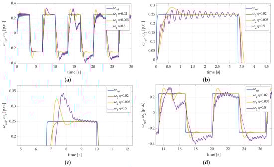
Figure 9.
Speed transients of the two-mass electric drive system with elastic shaft and SM-RBFNN controller with the time constant increased 3 times and different learning rate values: (a) a general overview of the simulation run; (b) a zoom-in showing the first steady-state transition; (c) a zoom-in showing third steady-state transition; (d) a zoom-in showing system stability loss.
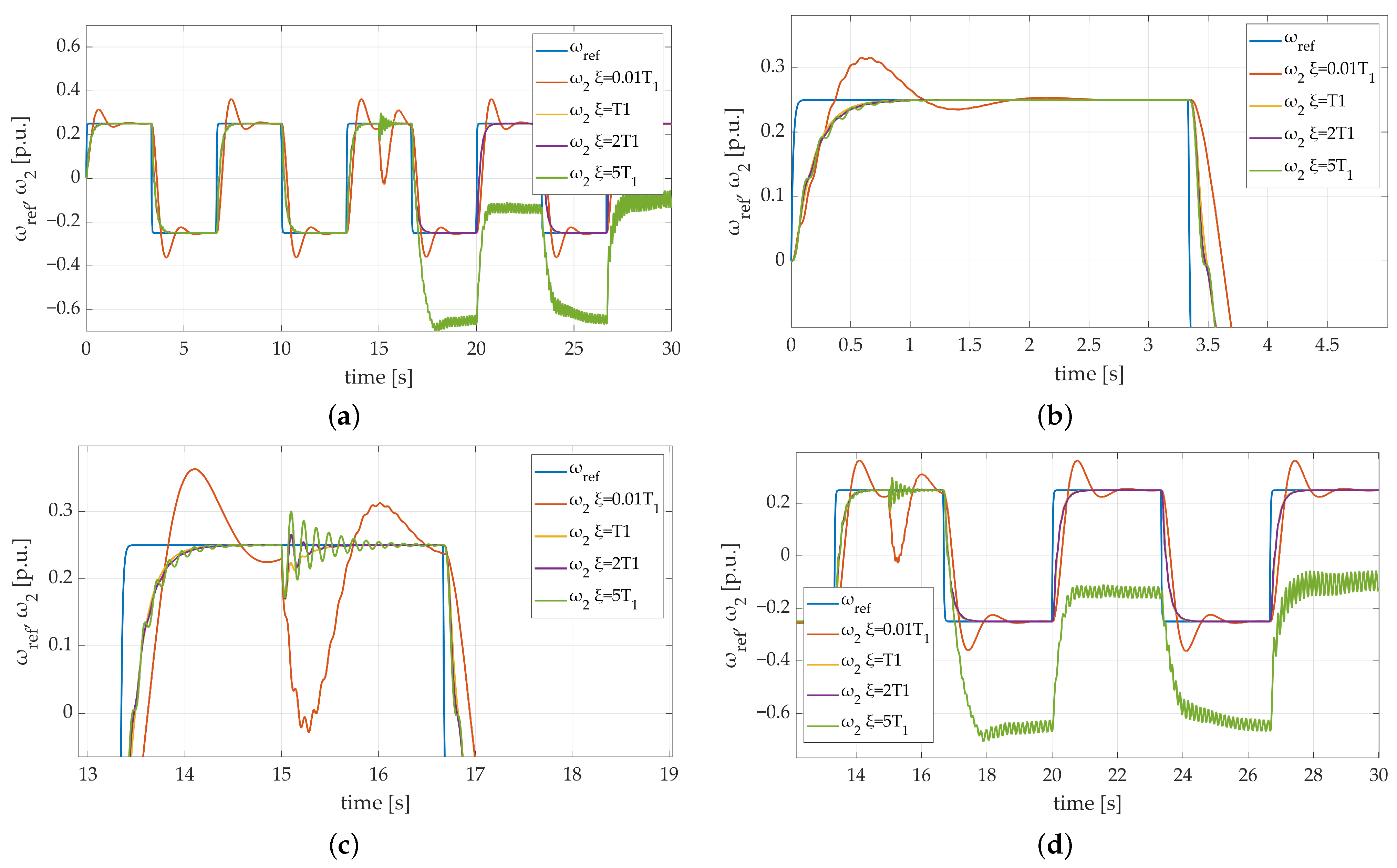
The fourth test was performed to examine the influence of gain value. The mentioned parameter is included in Equation (21). It is responsible for determining the influence of the error derivative contained in the sliding surface formula on the system response. The conducted test included four values of derivative gain: , , , . That test was also carried out with the load machine speed taken into consideration only. Obtained results are presented in Figure 10. Speed transients presented in Figure 10a,b confirm the fact that the error derivative gain has a significant influence on the overall dynamics of the system. Its low value () makes a visible overshoot after each return visible in the plant response. Moreover, Figure 10b proves that increasing the verified parameter influences system dynamics till a specific moment. As it is shown, there is no key difference in the slope steepness between the second, third, and fourth try. Nonetheless, the correct match of gain plays a crucial role in the system behavior. Figure 10c shows that too large a value of the examined coefficient not only makes the plant response fluctuate but also leads it to stability loss, which is considered an extremely dangerous situation. Summarizing the conducted test leads to the conclusion that the default gain value (considered as ) is marked with the best plant response. The steepness of the speed transient slope is high enough to ensure proper dynamics of the plant, no overshoots exist and what is even more essential, no stability loss was noticed. The obtained results demonstrate that in order to keep the satisfying dynamics of the system combined with its stable and predictable response the optimal derivative gain value needs to be found during the designing process.
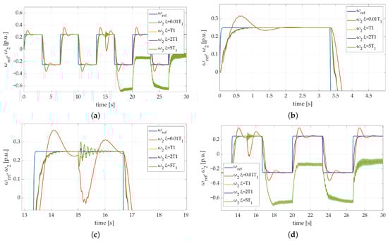
Figure 10.
Speed transients of the two-mass electric drive system with elastic shaft and SM-RBFNN controller with different speed error derivative gain: (a) a general overview of the simulation run; (b) a zoom-in showing the first steady-state transition; (c) a zoom-in showing the moment of additional load torque attachment; (d) a zoom-in showing adaptation progress between particular returns.
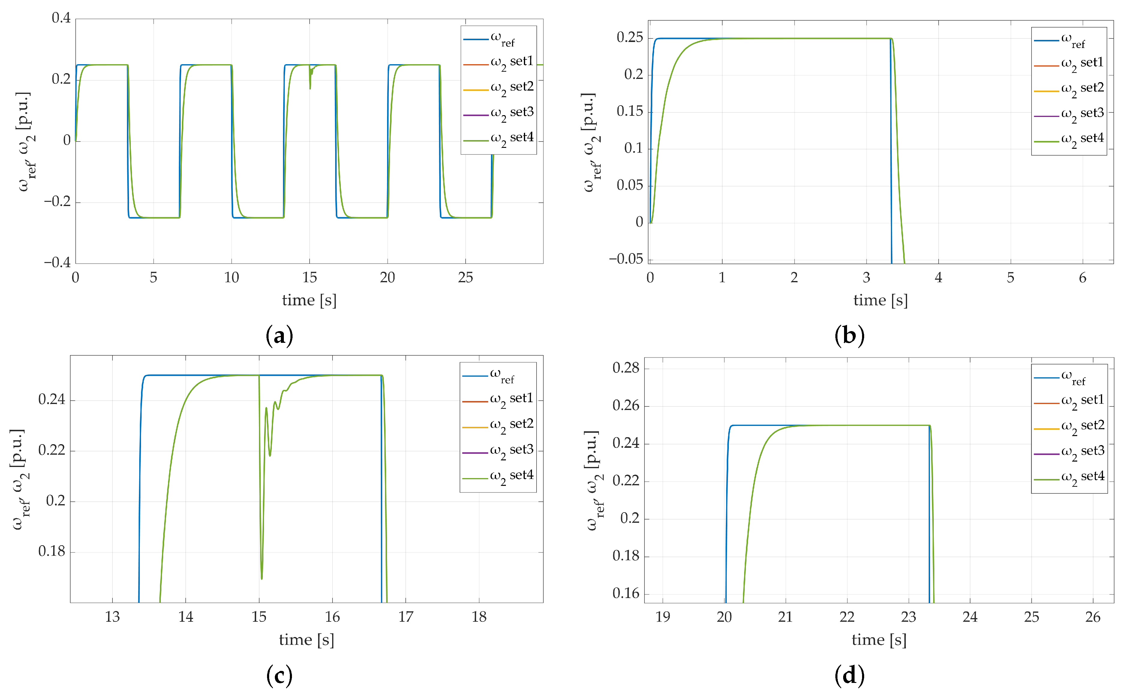
The last stage of the conducted simulations involved verifying the values of the initial weights’ influence on the system behavior. The dynamics of the system response and its robustness on additional load torque attachment were examined during the described attempt. To do so, four sets of initial weight coefficient values were prepared. To keep the stochastic nature of the chosen weight values, the rand function was used. The obtained results are shown in Figure 11. The presented speed transients prove that the difference in weight coefficient values may have a negligibly small impact on the system dynamics. It may be mainly visible right after enabling the drive system during reaching the first steady state or during additional load torque attachment. In the described test, no differences between obtained transients were noticed, which proves that the adaptation algorithm follows updated weight coefficients in a way that allows the control algorithm to follow the reference speed trajectory properly.
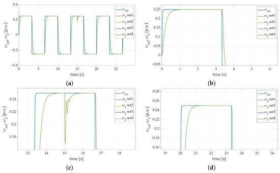
Figure 11.
Speed transients of the two-mass electric drive system with elastic shaft and SM-RBFNN controller with different sets of initial weight coefficient values: (a) a general overview of the simulation run; (b) a zoom-in showing the first steady-state transition; (c) a zoom-in showing the moment of additional load torque attachment; (d) a zoom-in showing convergence of actual and reference speed value for each case.
4. Experimental Results
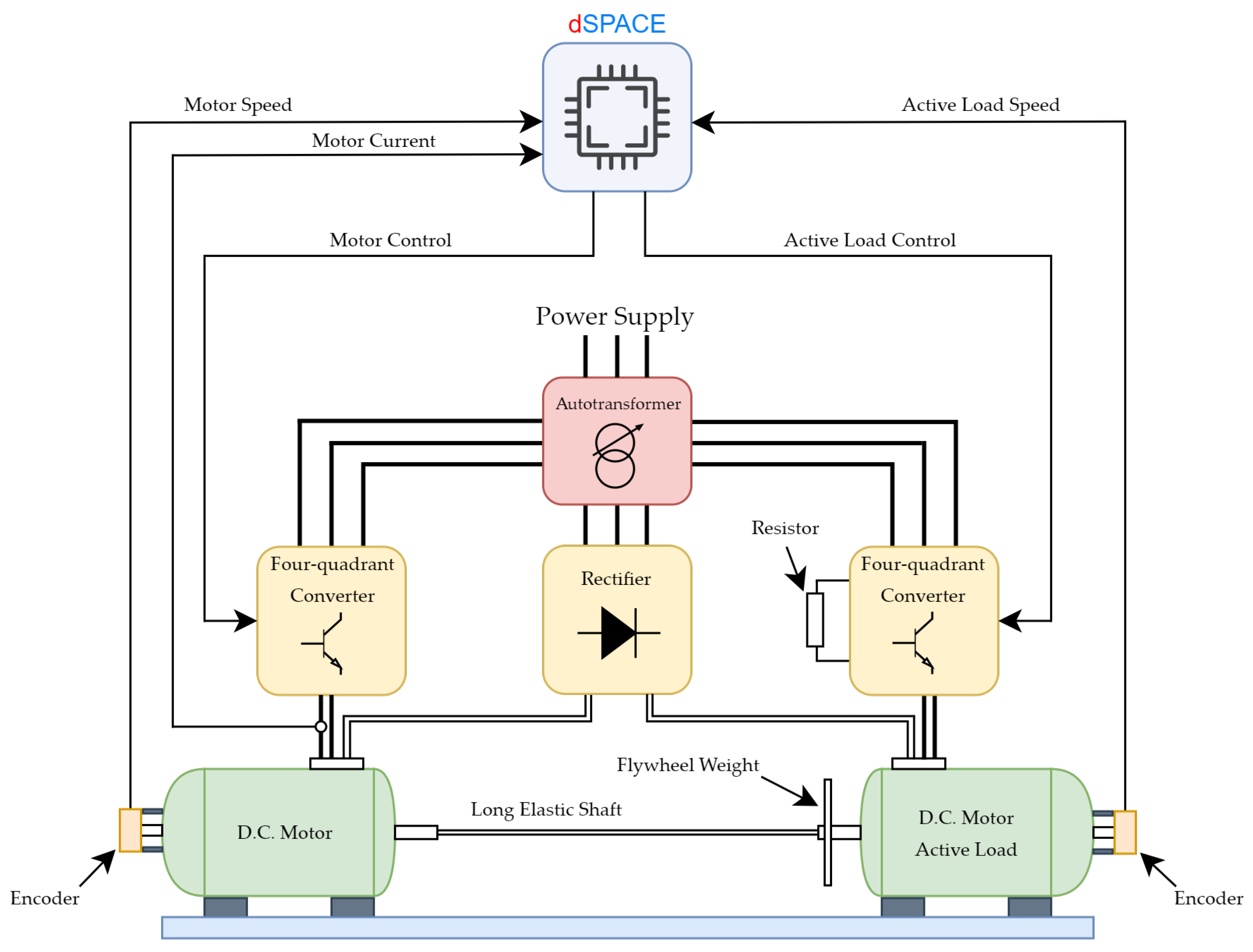
After finishing simulation tests with positive results, the next part involved carrying out experimental tests. The goal of that part was to confirm the propriety of the designed SM-RBFNN controller. To do so, two D.C. motor setups were used. The laboratory experimental setup contained one power supply in the form of an auto-transformer, two four-quadrant D.C.-D.C. converters, allowing the motor to rotate in two directions, and one rectifier. Because of the fact that second motor worked as an electric generator, an additional breaking resistor attached to its converter was required. The motors were coupled using a long, steel, elastic shaft. To simulate the change of the mechanical time constant of the machine, additional flywheel weight was attached. The whole experimental setup was controlled with the use of a 1103 dSPACE card equipped with a digital signal processor. Its role was to perform data acquisition of all speed and current signals, execute the control algorithm, and form proper PWM control signals. The overall structure of the experimental setup is shown in Figure 12.
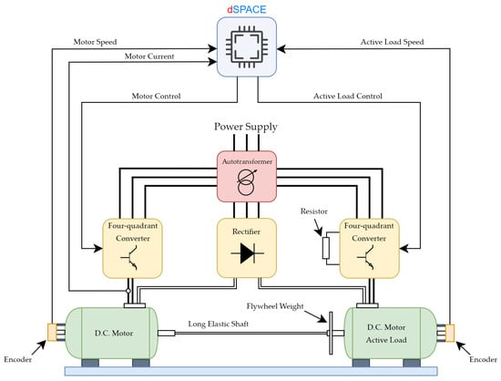
Figure 12.
Schematic diagram of experimental setup.
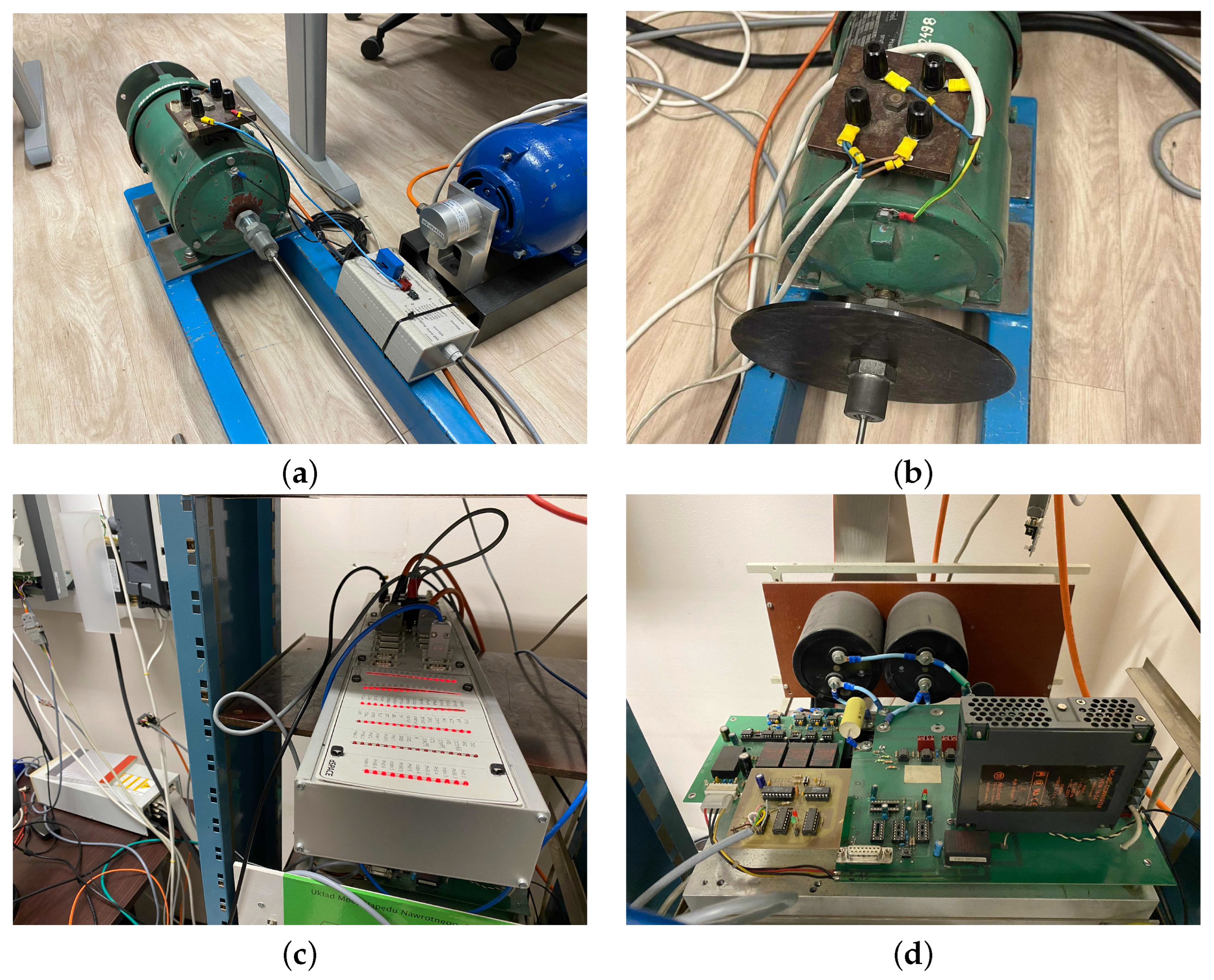
The basic parameters of the used setup are correlated in Table 1. The photos of particular components used in the experimental setup are shown in Figure 13.

Table 1.
Basic parameters of the used experimental setup.

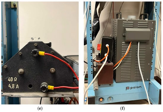
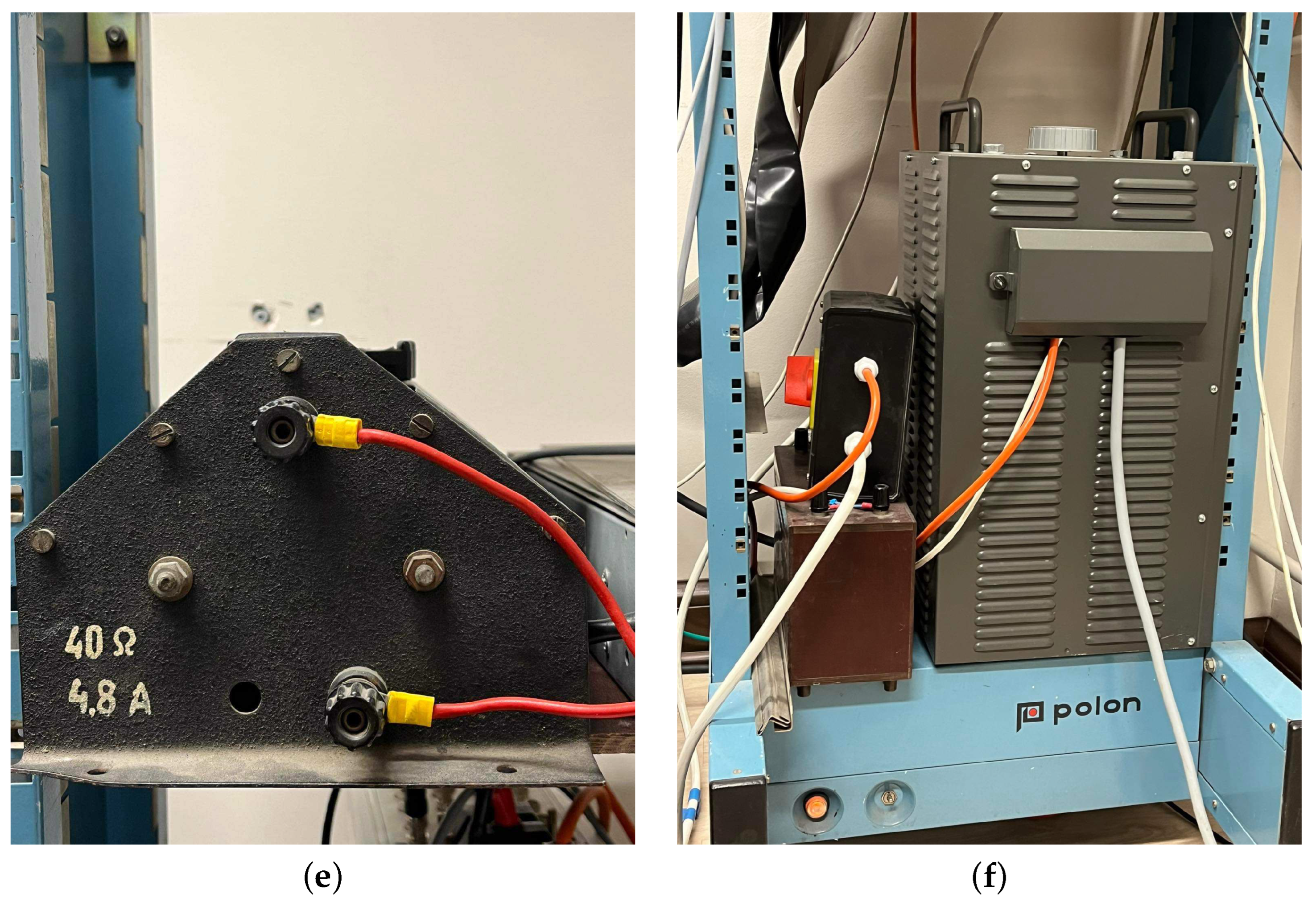
Figure 13.
Particular components of experimental setup: (a) D.C. motor with LEM current sensor; (b) D.C. load machine with flywheel weight attached; (c) 1103 dSPACE card; (d) four-quadrant D.C-D.C. converter; (e) resistor; (f) auto-transformer.
4.1. Verification of the SM-RBFNN Control Algorithm in Various Operating Conditions
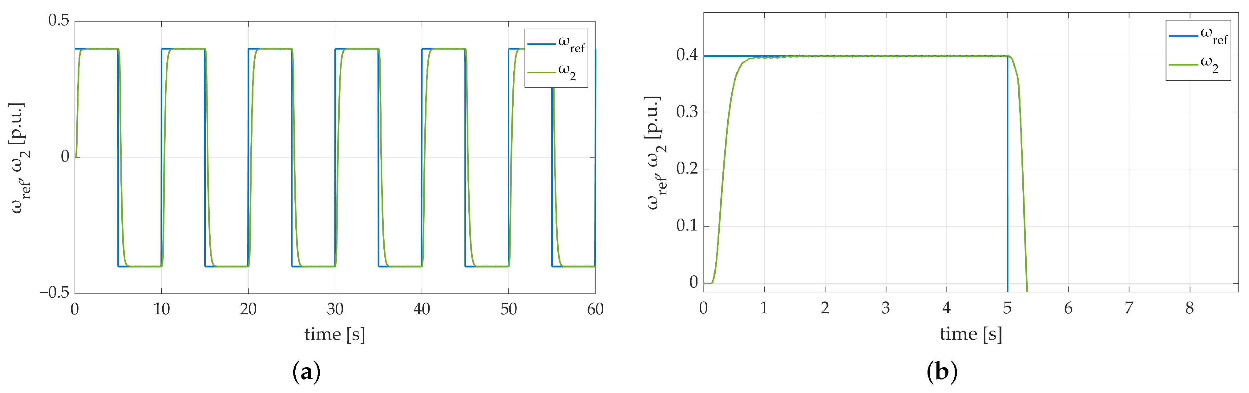
Four particular tests were distinguished in the experimental part. In the beginning, a default try was made to check whether the proposed controller could handle the basic parameters of the two-mass system. No additional torque disturbance and flywheel weight were used in this attempt (Figure 14a,b).
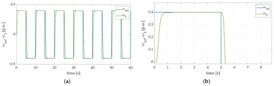
Figure 14.
Speed transients of the two-mass electric drive system with elastic shaft and SM-RBFNN controller obtained during the experiment: (a) neither additional load torque nor flywheel weight used; (b) neither additional load torque nor flywheel weight used-zoom-in showing the initial phase of the test.
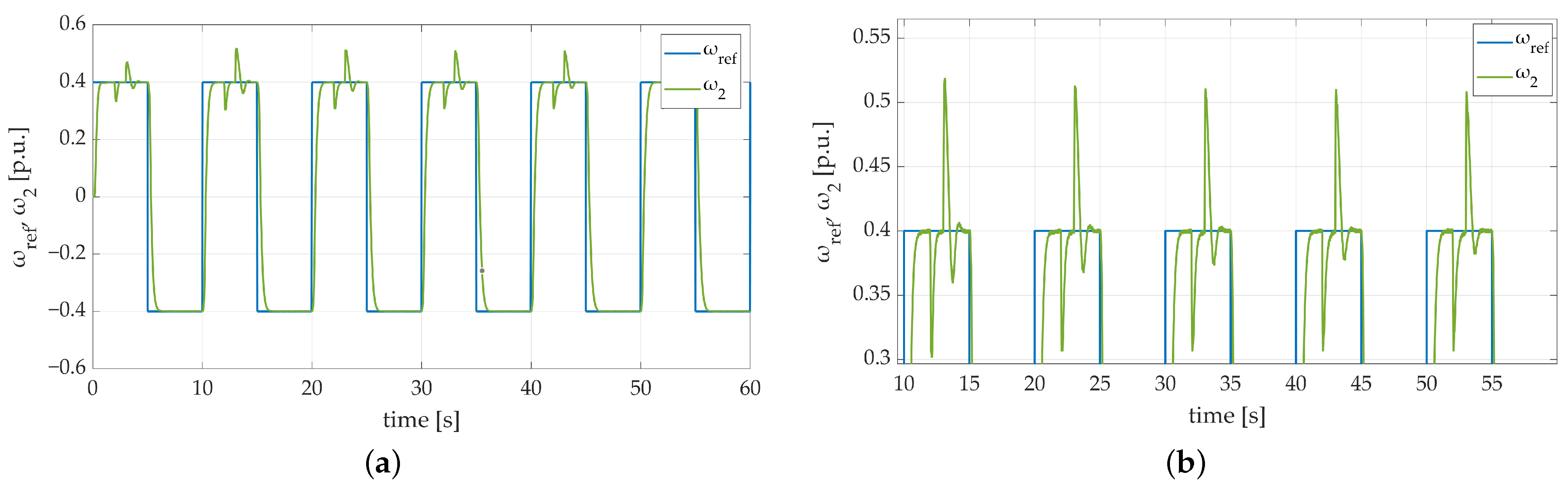
After achieving a positive system response, additional attempts were carried out. The first one included the use of active load torque (Figure 15a,b). Additional load torque was being attached during positive speed value only, then after the period of s it was switched off. Having analyzed the speed transient presented in Figure 15b it can be noticed that the adaptation algorithm works well. After each try when load torque occurs, the level of overshoots are progressively decreased.
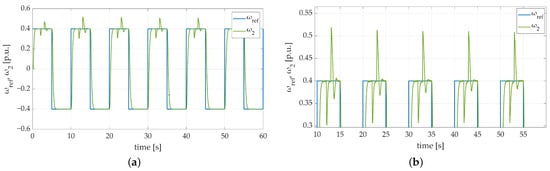
Figure 15.
Speed transients of the two-mass electric drive system with elastic shaft and SM-RBFNN controller obtained during the experiment: (a) active load torque with no fly-wheel weight; (b) active load torque with no fly-wheel weight—zoom-in showing the decreasing value of occurred overshoots.
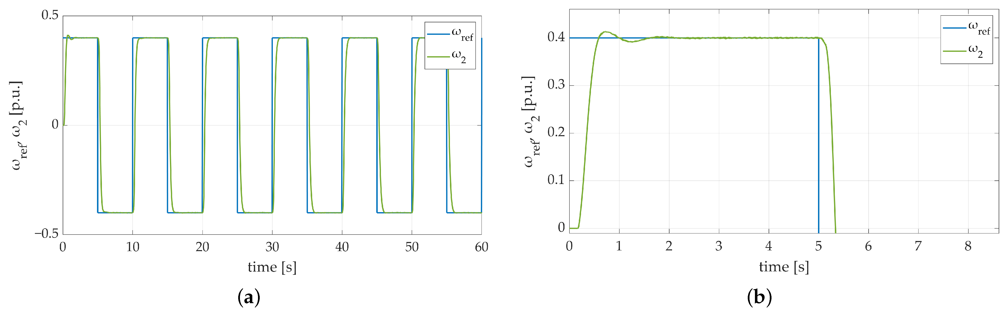
The third attempt included a lack of active torque load. Instead of the mentioned disturbance, a hypothetical mechanical time constant increase in the load machine was simulated. It was realized by putting an additional flywheel weight on the load machine’s part of the shaft. The attachment of the additional weight to the second motor caused its mechanical time constant to increase twice in regard to its default coefficient value. The obtained speed transients (Figure 16a,b) show that despite a small overshoot in the first steady-state transition, the adaptation algorithm works properly and converges the actual speed value to the reference signal.
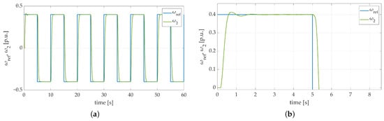
Figure 16.
Speed transients of the two-mass electric drive system with elastic shaft and SM-RBFNN controller obtained during the experiment: (a) single fly-wheel weight with no additional load torque; (b) single fly-wheel weight with no additional load torque—zoom-in showing the initial phase of the test.
Afterwards, the most complex attempt was made. Besides having additional flywheel weight installed on the load machine’s shaft, active load torque was applied as well. The obtained results are presented in Figure 17a,b. Likewise, the quality of the SM-RBFNN controller work is satisfactory. The adaptation algorithm gradually decreases the value of the overshoot occurring after switching off the external load torque every single try. Moreover, the actual speed value converges to the reference signal, which at this point confirms the robustness of the designed control structure.
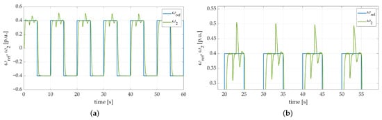
Figure 17.
Speed transients of the two-mass electric drive system with elastic shaft and SM-RBFNN controller obtained during the experiment: (a) both additional load torque and single flywheel weight applied; (b) both additional load torque and single flywheel weight applied—zoom-in showing decreasing values of the overshoots that occurred.
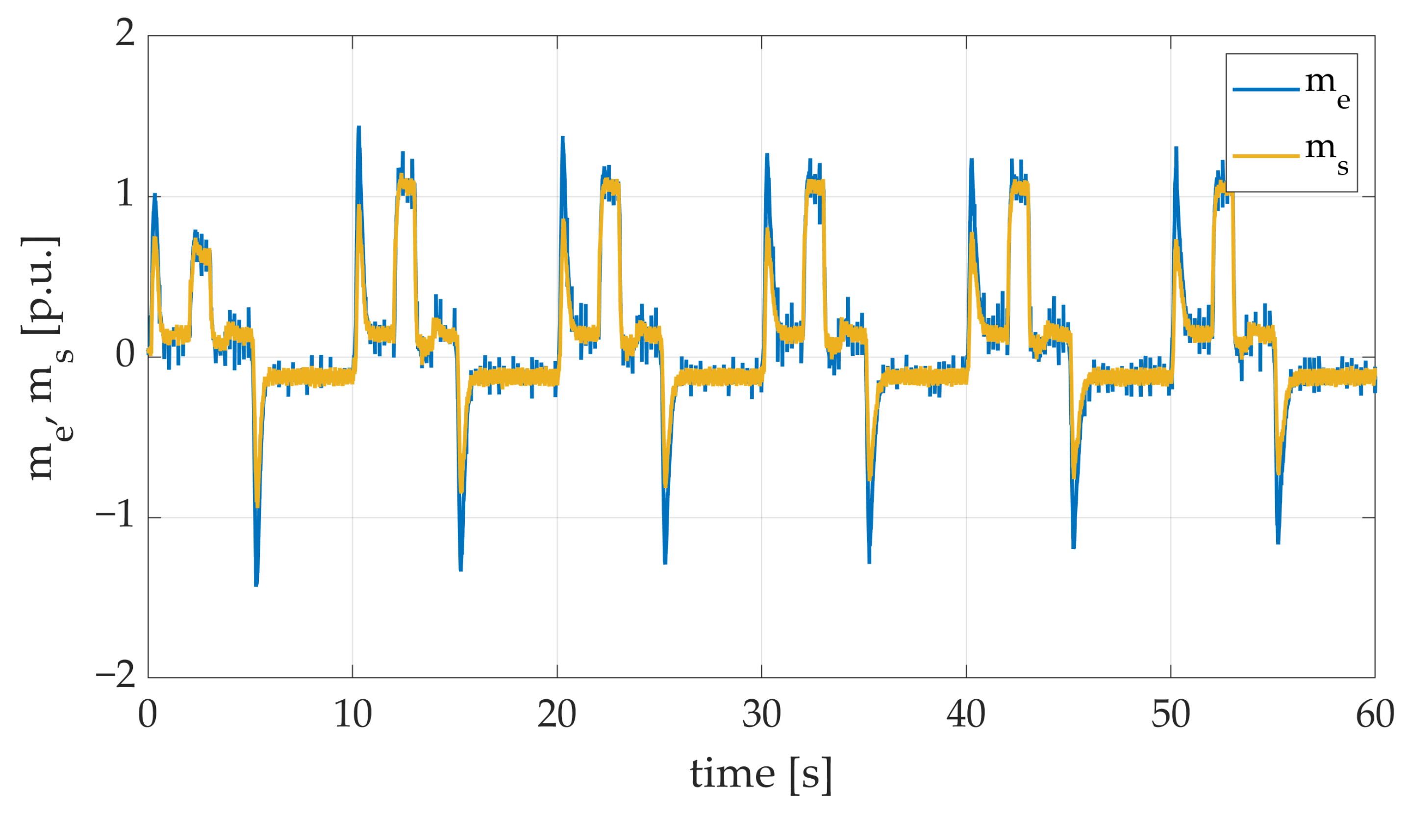
Furthermore, the obtained transients of electromagnetic and torsional torque included in Figure 18 confirm that the behavior of the control system and its reaction to active load torque are accurate. The presented results clearly demonstrate the moment of additional load torque attachment. The analysis of electromagnetic and torsional torque confirms the stability of the system.

Figure 18.
Electromagnetic and torsional torque transients of the two-mass electric drive system with elastic shaft and SM-RBFNN controller obtained during the experiment with both additional load torque and single flywheel weight applied.
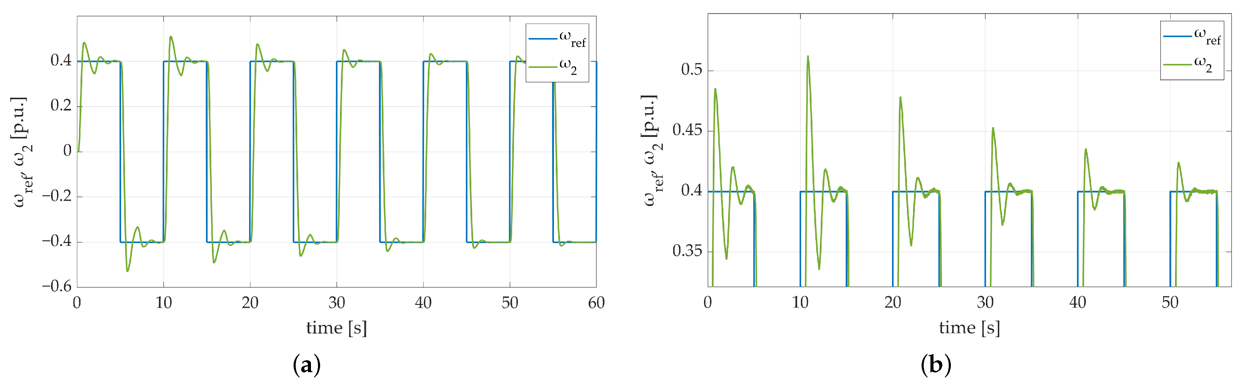
The second stage of the conducted experimental tests was focused on increasing the mechanical time constant of the load machine by changing the type of applied flywheel weight. The mechanical time constant of the additional wheel used in the second test equals . The first try involved a general overview of the system behavior. The results, presented in Figure 19 illustrate that the system response is valid. The speed transient presented in Figure 19b proves the efficiency of the implemented adaptation algorithm. The occurring overshoots are gradually minimized after every single return.
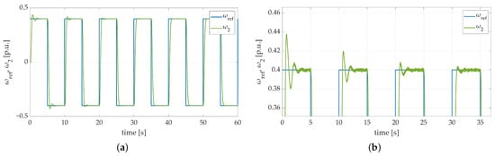
Figure 19.
Speed transients of the two-mass electric drive system with elastic shaft and SM-RBFNN controller obtained during the experiment: (a) double fly-wheel weight with no additional load torque; (b) double fly-wheel weight with no additional load torque—zoom-in showing the initial phase of the test.
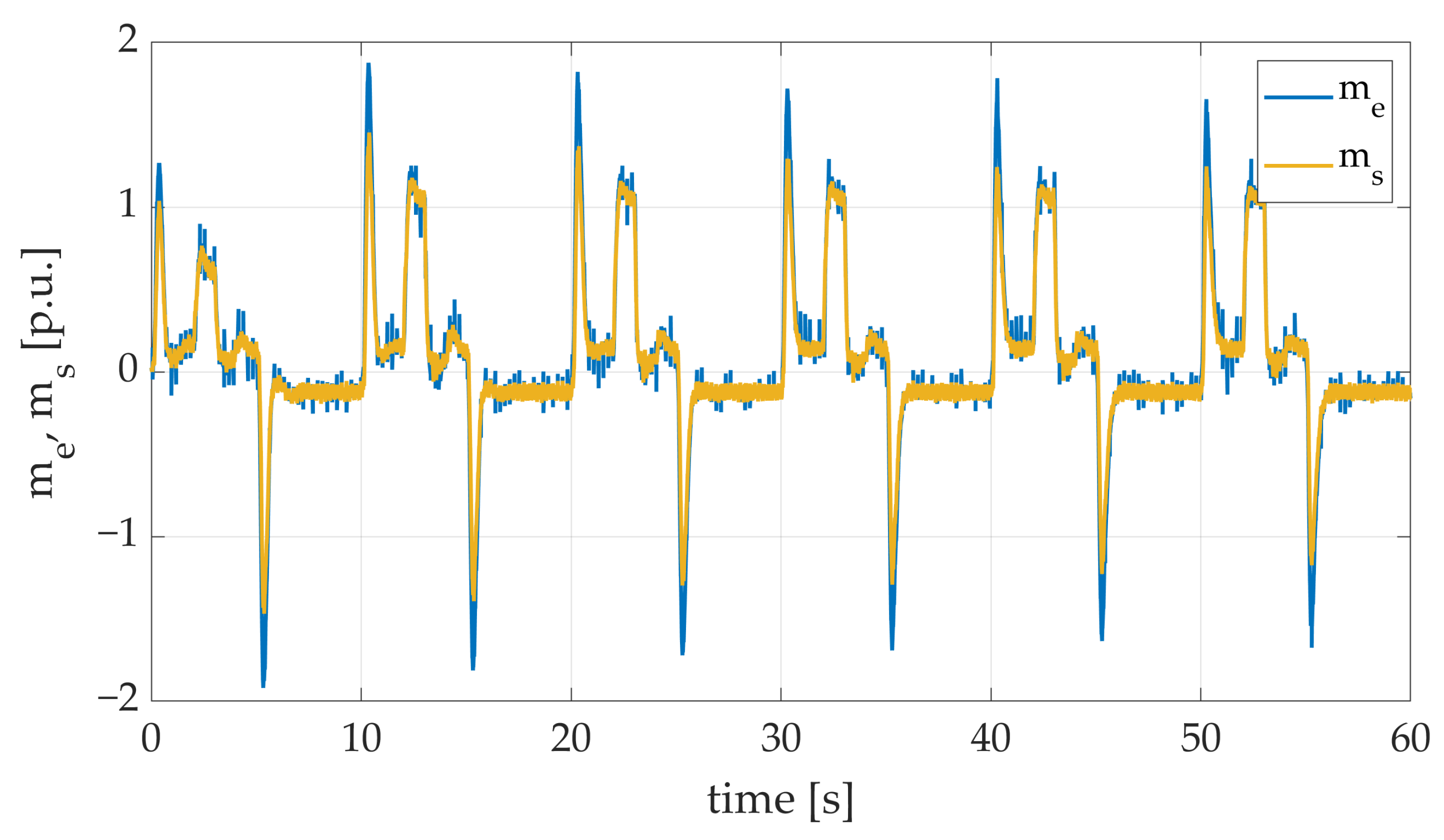
The next attempt included additional active load torque attachment. The parameters of the additional load stayed the same compared to the first stage of the experiment. The obtained results are shown in Figure 20. Due to the increased load machine mechanical time constant, overshoots are characterized by a significantly bigger amplitude. However, the implemented control system with an integrated adaptation algorithm regularly mitigates the mentioned effect. It can be noticed that the proposed structure deals with significant mechanical time constant changes effectively. The electromagnetic torque transient presented in Figure 21 demonstrates a significant increase in absolute value growth due to big mechanical time constant growth. Despite the mentioned parameter change the system remains stable.
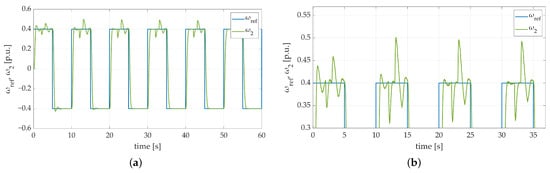
Figure 20.
Speed transients of the two-mass electric drive system with elastic shaft and SM-RBFNN controller obtained during the experiment: (a) both additional load torque and double flywheel-weight applied, (b) both additional load torque and double flywheel-weight applied—zoom-in showing decreasing values of occurred overshoots.
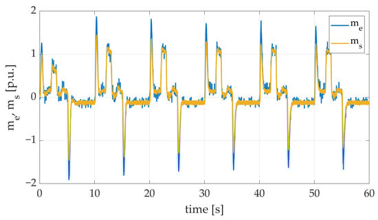
Figure 21.
Electromagnetic and torsional torque transients of the two-mass electric drive system with elastic shaft and SM-RBFNN controller obtained during the experiment with both additional load torque and double flywheel weight applied.
The last part of experimental tests stage covered the examination of the proposed algorithm in terms of extremely changed parameters of the plant. To do so, the third flywheel weight was attached to the load machine. The increase in its mechanical time constant could be described as , which resulted in a five times bigger inertia of the electric generator with regard to its default parameters. In this particular try, it was crucial not to activate additional load torque in order to keep the shaft unbroken. The obtained results are presented in Figure 22. Furthermore, a huge increase in load mechanical time constant caused a significant rise of electromagnetic torque, visible in Figure 23. Despite having observed substantial overshoots after the first returns of the drive, it is undeniably visible that the proposed control algorithm handles the extreme mechanical time constant increase. The conducted test leads to the conclusion that the designed control strategy features high robustness combined with distinguished adaptation capabilities.
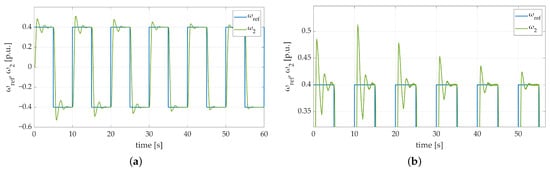
Figure 22.
Speed transients of the two-mass electric drive system with elastic shaft and SM-RBFNN controller obtained during the experiment: (a) 4-times bigger fly-wheel weight with no additional load torque; (b) 4-times bigger fly-wheel weight with no additional load torque—zoom-in showing the initial phase of the test.
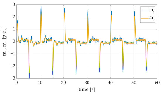
Figure 23.
Electromagnetic and torsional torque transients of the two-mass electric drive system with elastic shaft and SM-RBFNN controller obtained during the experiment with four mechanical machine load time constant values flywheel-weight applied.
4.2. Comparative Study of the Proposed Sliding Mode-Radial Basis Function Neural Network-Based Controller
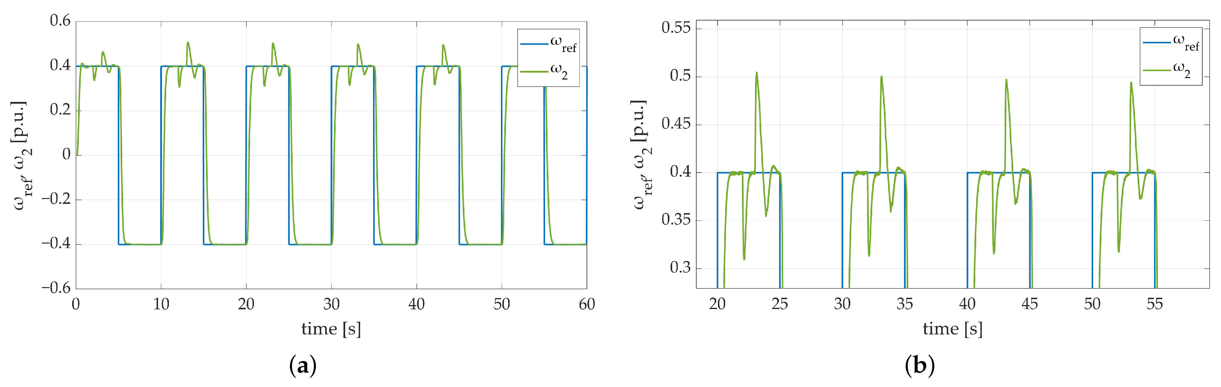
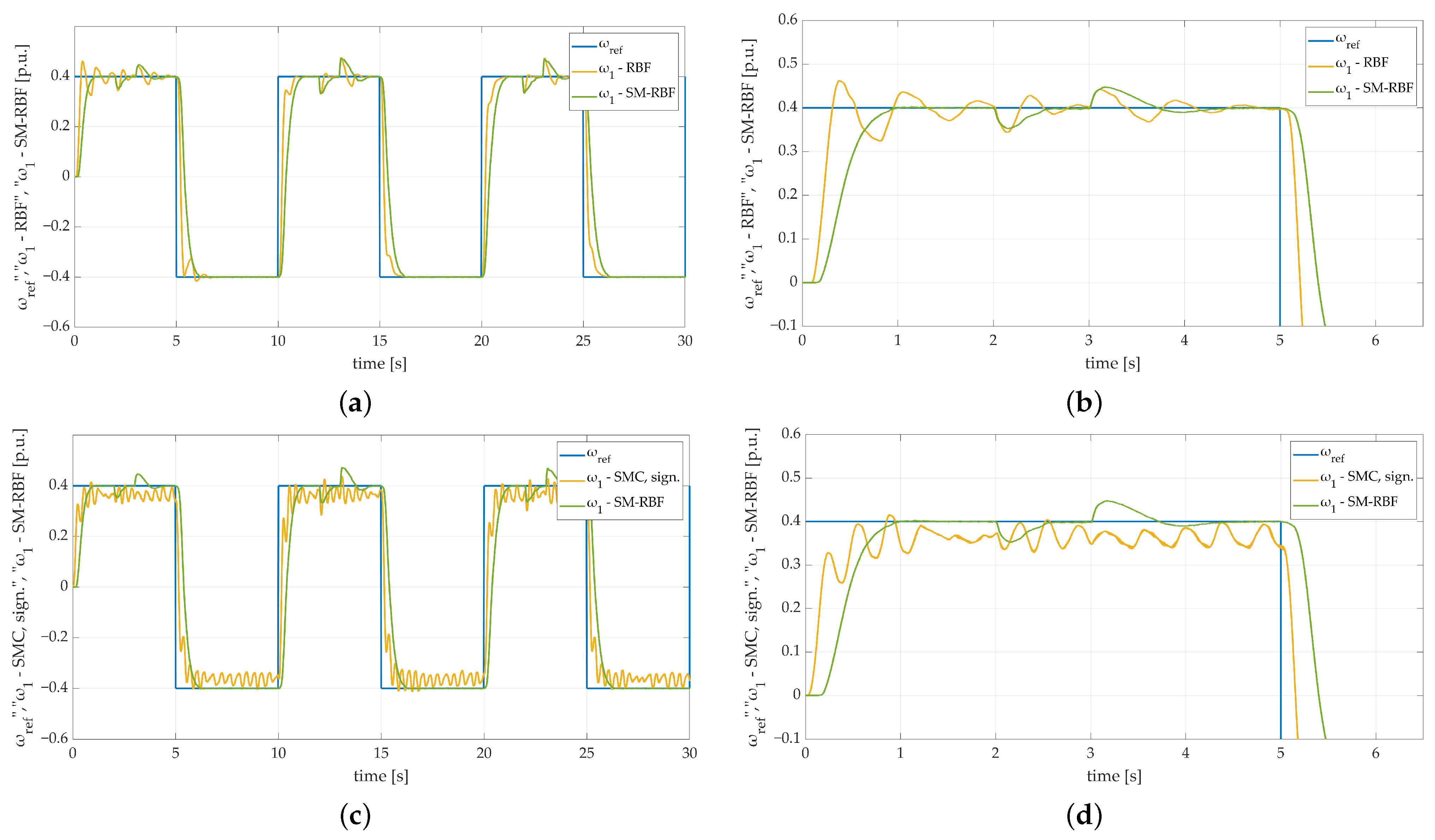
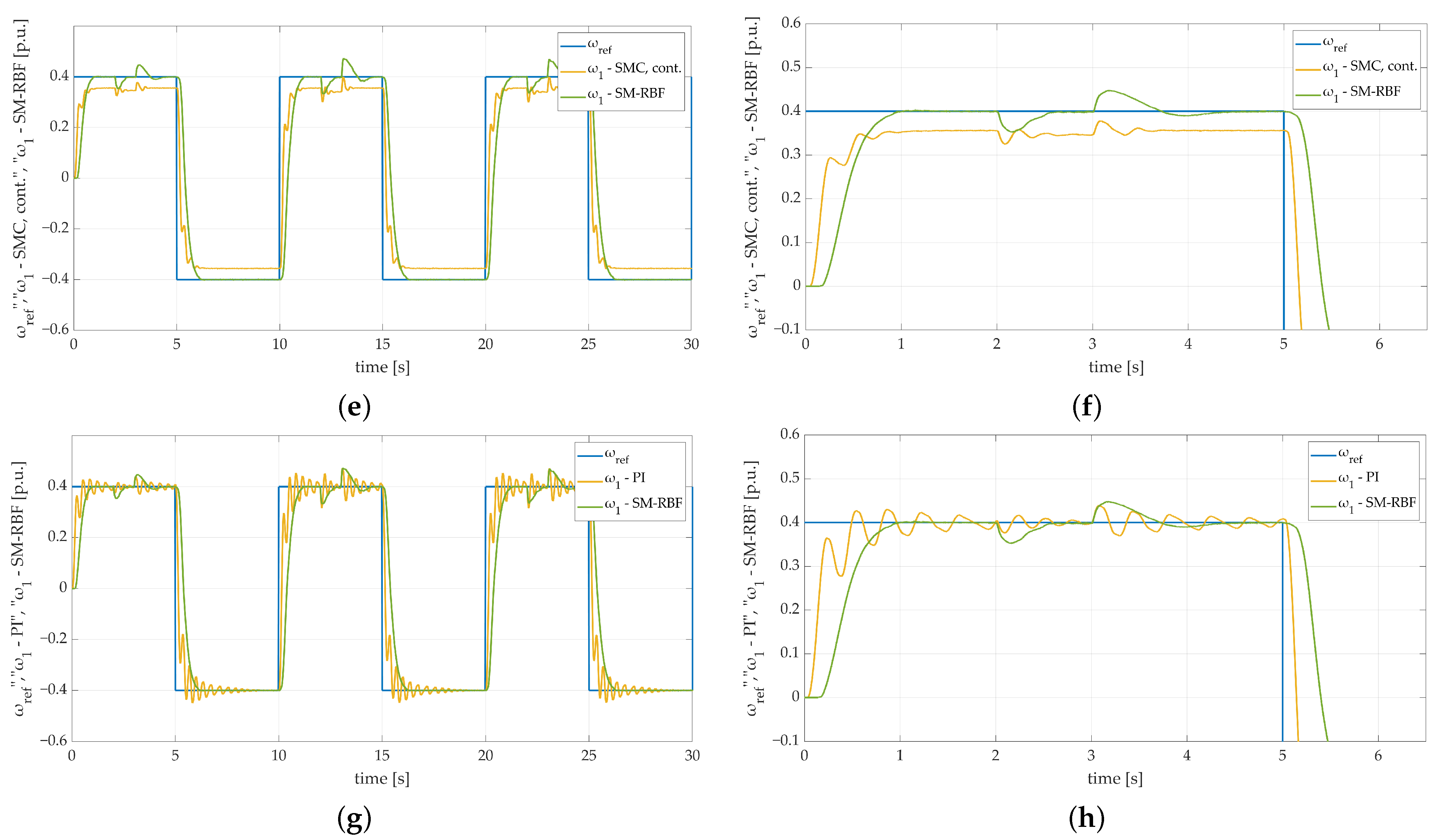
The experiments conducted in Section 4 showed that the validity of the proposed structure has been proven. The examined algorithm features high robustness and efficient adaptation capabilities, which make it a feasible and versatile solution for speed control loops dedicated to complex mechanical systems. However, in order to confirm the fact, that the proposed controller can be considered as a sound and competitive solution for such mechanical systems, additional tests have been conducted. In the comparison, the SM-RBFNN controller is examined alongside controllers already known from the literature: conventional sliding mode controller (deployed using both continuous function (cont.) and signum function (sign.)), RBFNN functioning as a speed controller, and a traditional PI controller. Considering the fact that the main difficulty is related to variable parameters of the plant, the conducted tests include the increased value of load machine mechanical time constant with the use of single flywheel weight (). That being said, it is crucial to mention, that the objectivity of additional tests required controllers tuning processes to be conducted with regard to the nominal time constant. The obtained results are shown in Figure 24. The comparison of the presented transients clearly proves that the proposed SM-RBFNN controller can be considered a reliable solution in terms of speed regulation in complex, mechanical systems with changeable parameters.
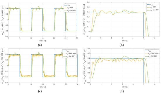
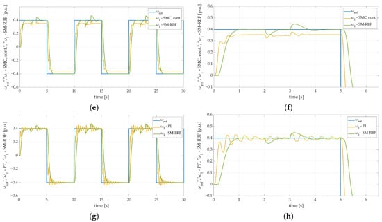
Figure 24.
Speed transients of the two-mass electric drive system with the elastic shaft, different controllers, single fly-wheel weight, and additional torque load obtained during the experiment: (a) RBFNN controller; (b) RBFNN controller—zoom-in showing first steady-state transition, (c) SMC controller with sign. function, (d) SMC controller with sign. function—zoom-in showing first steady-state transition, (e) SMC controller with cont. function, (f) SMC controller with cont. function—zoom-in showing first steady-state transition, (g) PI controller, (h) PI controller—zoom-in showing steady-state transition.
The main purpose of the conducted experiments was to compare the dynamics of the system obtained with the use of the proposed algorithm with conventional, competitive controllers. The speed transients presented in Figure 24a,b present convergence of reference signal with actual load machine speed. However, despite the fact, that conventional RBFNN with error-based input signal handles speed control loop satisfactorily, the difference between the first steady-state settling times is conspicuous. The obtained response is significantly worse compared to the proposed SM-RBFNN controller.
The typical sliding mode controller does not ensure actual speed convergence with its reference trajectory. The obtained results are insufficient, regardless of the control law function. Figure 24c,d clearly show that the obtained speed transient exemplifies typical inconveniences of sliding mode control strategy. Both chattering and steady-state error occurred, which makes the use of conventional SM controller in such mechanical systems unacceptable.
Substituting the signum switching function with a continuous (saturation) one casued the chattering effect to significantly diminish. Nevertheless, the steady-state error is still a major issue in the presented control strategy.
The last stage of additional tests contained a comparison between SM-RBFNN and linear PI controller. Speed transients shown in Figure 24g,h demonstrate that the PI controller does not ensure acceptable results in terms of two-mass systems speed control. The oscillations that occurred are not damped, which can be a serious inconvenience. Not only may it lead to mechanical failure of the system, but it can also be a reason for sudden system stability loss.
Summarizing the conducted comparison, additional speed transients are presented. The obtained results prove that the proposed algorithm eliminates typical sliding mode control inconveniences while ensuring significant dynamics improvement.
5. Conclusions and Results Discussion
In this article, a sliding surface radial basis function neural network speed controller applied to two-mass system speed control is proposed. The main contribution of this paper is that the RBFNN is utilized as a switching function for two tasks: chattering minimization and adaptive action. Experimental studies show the prevalence of the proposed control strategy over other conventional solutions. Lyapunov stability proof is first derived to achieve the criteria that need to be fulfilled in order for the system to be safe and operational. Numerical studies show the expected control system behavior. The sliding surface is followed in a gentle fashion, providing a smooth and non-oscillatory step response. The impact of all the adjustable parameters of the algorithm is examined to verify their relevance and facilitate the tuning process. The tests performed on the experimental bench confirm the findings from the simulations. The following advantages have been achieved through the use of the proposed SM-RBFNN controller:
- The system shows robustness against parametric uncertainty. Even though many non-linear phenomena, such as backlash, friction, and misalignment, were not included in the two-mass system description from Equation (1), the experimental tests show no significant divergence from the numerical studies (compare Figure 6 and Figure 14).
- Convergence of the RBFNN training is proven through the adaptive properties that can be seen in the latter figures in the experimental section of the manuscript. The oscillatory response that results from the increased inertia of the load machine is gradually mitigated as the weights are adjusted to the current state of the drive.
- The control system’s response to the active loading provided by the load machine is also adjusted by the neural network. The undershoots and overshoots resulting from the load torque being activated and deactivated are continuously being minimized. This shows that the learning process adapts the RBFNN to both parametric uncertainties and external disturbances.
- Another advantage that can be observed from the use of the RBFNN is the elimination of chattering that is normally observed with sliding-mode control structures with a signum switching function at the output of the controller.
- Elimination of oscillations and mitigation of overshoot is a great finding considering the fact that the control structure does not receive any additional information about the state of the drive. Only the information about the angular speed of the motor is provided. Neither the motor current, speed of the load nor torsional torque need to be measured/estimated. This feature creates a great opportunity to lower the cost and enhance the reliability of the drive. With the limited amount of needed information, the proposed control algorithm is not computationally heavy and does not rely on the estimation of variables unavailable for measurement. Both of these features enable the possibility to use more affordable programmable devices to determine the switching signals for the power electronics. Also, with fewer measuring devices, drive maintenance becomes much more feasible, and detection of faults is simplified due to a limited number of elements to be monitored.
The values of the parameters of the control structure were adjusted arbitrarily, solely based on the findings from the numerical tests. Therefore, further improvement can be expected if these values are optimized. For this purpose, e.g., a nature-inspired algorithm could be implemented. Nevertheless, the results shown in the manuscript present promising points of development for electric drives with flexible links.
Author Contributions
Conceptualization, M.K.; methodology, M.K., G.K. and R.S.; software, G.K. and R.S.; validation, M.K., G.K., R.S. and J.S.; formal analysis, M.K., G.K., R.S. and J.S.; investigation, M.K., G.K. and R.S.; data curation, G.K. and R.S.; writing—original draft preparation, M.K., G.K., R.S. and J.S.; writing—review and editing, M.K., G.K., R.S. and J.S.; visualization, G.K. and R.S.; supervision, M.K.; project administration, M.K. All authors have read and agreed to the published version of the manuscript.
Funding
This research received no external funding.
Institutional Review Board Statement
Not applicable.
Informed Consent Statement
Not applicable.
Data Availability Statement
Data are contained within the article.
Conflicts of Interest
The authors declare no conflicts of interest.
Abbreviations
The following abbreviations are used in this manuscript:
| MRAS | Model Reference Adaptive System |
| RBFNN | Radial Basis Function Neural Network |
References
- Ferdousee, A. Impact of Electric Vehicle Adoption on Electricity Consumption and Generation: Evidence from California. Int. J. Energy Econ. Policy 2022, 12, 101–110. [Google Scholar] [CrossRef]
- Ta, J.; Song, C.; Han, H.; Li, Y. Effects of Flexibility and Suspension Configuration of Main Shaft on Dynamic Characteristics of Wind Turbine Drivetrain. Chin. J. Mech. Eng. 2019, 32, 36. [Google Scholar] [CrossRef]
- Liu, H.; Zhao, R.Z. Dynamic Error Analsis Based on Flexible Shaft of Wind Turbine Gearbox. IOP Conf. Ser. Mater. Sci. Eng. 2013, 52, 052015. [Google Scholar] [CrossRef]
- Zouari, L.; Abid, H.; Abid, M. Sliding Mode and PI controllers for uncertain flexible joint manipulator. Int. J. Autom. Comput. 2015, 12, 117–124. [Google Scholar] [CrossRef]
- Dong, X.; Shi, K.; Li, W. Residual vibration control of a single-link flexible manipulator with variable stiffness and damping magnetorheological joint. J. Phys. Conf. Ser. 2020, 1678, 012005. [Google Scholar] [CrossRef]
- Alam, W.; Mehmood, A.; Ali, K.; Javaid, U.; Alharbi, S.A.; Iqbal, J. Nonlinear Control of a Flexible Joint Robotic Manipulator with Experimental Validation. Stroj.-Vestn.—J. Mech. Eng. 2018, 64, 47–55. [Google Scholar] [CrossRef]
- Wang, B.; Lou, J. Coupling dynamic modelling and parameter identification of a flexible manipulator system with harmonic drive. Meas. Control 2019, 52, 122–130. [Google Scholar] [CrossRef]
- Zhang, S.; Zhang, X.; Sun, Z. An Improved Super-Twisting Sliding Mode for Flexible Upper-Limb Exoskeleton. Actuators 2023, 12, 32. [Google Scholar] [CrossRef]
- Chen, X. Robot dynamic trajectory tracking control algorithm based on steady-state closed-loop learning. J. Phys. 2020, 1682, 012069. [Google Scholar] [CrossRef]
- Lingzhen, S.; Shuo, Y.; Yunsheng, C. Dynamic Load Rejection Control Method for Flexible Space Manipulator. In Proceedings of the 3rd International Conference on Mechatronics and Information Technology (ICMIT 2018), Chengdu, China, 30–31 October 2018. [Google Scholar] [CrossRef]
- Carabis, D.S.; Wen, J.T.Y. Trajectory Generation for Flexible-Joint Space Manipulators. Front. Robot. AI 2022, 9, 687595. [Google Scholar] [CrossRef]
- Shao, M.; Huang, Y.; Silberschmidt, V.V. Intelligent Manipulator with Flexible Link and Joint: Modeling and Vibration Control. Shock Vib. 2020, 2020, 4671358. [Google Scholar] [CrossRef]
- Ata, A.A.; Johar, H. Dynamic simulation of task constrained of a rigid-flexible manipulator. Int. J. Adv. Robot. Syst. 2004, 1, 6. [Google Scholar] [CrossRef]
- Xiaolei, Z.; Yanbo, W.; Ke, L.; Shanda, W. Research on the motion characteristics of a flexible joint-flexible link space manipulator. In Proceedings of the 8th International Symposium on Vehicle Emission Supervision and Environment Protection (VESEP2022), Wuhan, China, 23–24 June 2022; p. 01061. [Google Scholar] [CrossRef]
- Lee, S.H.; Lee, C.W. Hybrid Control Scheme for Robust Tracking of Two-Link Flexible Manipulator. J. Intell. Robot. Syst. 2002, 34, 431–452. [Google Scholar] [CrossRef]
- Kchaou, M.; Al Ahmadi, S.; Draou, E. Integral Sliding-Mode Fault-Tolerant Control for Fuzzy Singular Systems with Actuator Saturation. Circuits, Syst. Signal Process. 2020, 39, 1307–1334. [Google Scholar] [CrossRef]
- Kchaou, M.; Jerbi, H. Reliable H∞ and Passive Fuzzy Observer-Based Sliding Mode Control for Nonlinear Descriptor Systems Subject to Actuator Failure. Int. J. Fuzzy Syst. 2022, 24, 105–120. [Google Scholar] [CrossRef]
- Jinyong, J.; Zhao, Y.; Zhang, C.; Liu, Y. Vibration Suppression of a Flexible-Joint Robot Based on Parameter Identification and Fuzzy PID Control. Algorithms 2018, 11, 189. [Google Scholar] [CrossRef]
- Zhang, Y.; Pang, A.; Zhu, H.; Feng, H. Structured H∞ Control for Spacecraft with Flexible Appendages. Entropy 2021, 23, 930. [Google Scholar] [CrossRef]
- Kharabian, B.; Mirinejad, H. Hybrid Sliding Mode/H-Infinity Control Approach for Uncertain Flexible Manipulators. IEEE Access 2020, 8, 170452–170460. [Google Scholar] [CrossRef]
- Akbari, M.E.; Badamchizadeh, M.A.; Poor, M.A. Implementation of a Fuzzy TSK Controller for a Flexible Joint Robot. Discret. Dyn. Nat. Soc. 2012, 2012, 279498. [Google Scholar] [CrossRef]
- Verma, V.; Chauhan, S. Adaptive PID-Fuzzy Logic Controller for Brushless DC Motor. In Proceedings of the 2019 3rd International conference on Electronics, Communication and Aerospace Technology (ICECA), Coimbatore, India, 12–14 June 2019; pp. 445–449. [Google Scholar] [CrossRef]
- Alset, U.; Apte, A.; Mehta, H. Implementation of Fuzzy Logic based High Performance Speed Control System for PMDC motor using ATMEGA-328P-PU Micro-controller. In Proceedings of the 2020 IEEE International Conference on Electronics, Computing and Communication Technologies (CONECCT), Bangalore, India, 2–4 July 2020; pp. 1–5. [Google Scholar] [CrossRef]
- Shao, Z.; Tang, X.; Wang, L.; You, Z. A Fuzzy PID Approach for the Vibration Control of the FSPM. Int. J. Adv. Robot. Syst. 2013, 10, 59. [Google Scholar] [CrossRef]
- Reddy, V.; Venkateswararao, B.; Knypiński, Ł.; Devarapalli, R. Sizing of the Switched Reluctance Motor for Electric Vehicles. In Proceedings of the 2023 Progress in Applied Electrical Engineering (PAEE), Koscielisko, Poland, 26–30 June 2023; pp. 1–4. [Google Scholar] [CrossRef]
- Kaminski, M. Neural Network Training Using Particle Swarm Optimization—A Case Study. In Proceedings of the 2019 24th International Conference on Methods and Models in Automation and Robotics (MMAR), Miedzyzdroje, Poland, 26–29 August 2019; pp. 115–120. [Google Scholar] [CrossRef]
- M, S.; P, S.; K, N.G. Fuzzy Logic Controller Based BLDC Motor Control for Propulsion Application. In Proceedings of the 2022 IEEE International Power and Renewable Energy Conference (IPRECON), Kollam, India, 16–18 December 2022; pp. 1–6. [Google Scholar] [CrossRef]
- Samantaray, J.; Chakrabarty, S. Implementing sliding mode control of DC servo motor over a control network. In Proceedings of the 2018 Indian Control Conference (ICC), Kanpur, India, 4–6 January 2018; pp. 358–362. [Google Scholar] [CrossRef]
- El-Sousy, F.F.M.; Amin, M.M.; Mohammed, O.A. Robust Adaptive Neural Network Tracking Control with Optimized Super-Twisting Sliding-Mode Technique for Induction Motor Drive System. IEEE Trans. Ind. Appl. 2022, 58, 4134–4157. [Google Scholar] [CrossRef]
- Liu, Y.C.; Laghrouche, S.; N’Diaye, A.; Cirrincione, M. Hermite neural network-based second-order sliding-mode control of synchronous reluctance motor drive systems. J. Frankl. Inst. 2021, 358, 400–427. [Google Scholar] [CrossRef]
- Zhang, L.; Mahmoud, G.; Li, M.; Chen, Y. Robust Sliding Mode Controller with Suppressor for DC Motor System with Disturbances. In Proceedings of the 2019 Chinese Automation Congress (CAC), Hangzhou, China, 22–24 November 2019; pp. 1676–1681. [Google Scholar] [CrossRef]
- Murali, S.B.; Rao, P.M. Adaptive sliding mode control of BLDC motor using cuckoo search algorithm. In Proceedings of the 2018 2nd International Conference on Inventive Systems and Control (ICISC), Coimbatore, India, 19–20 January 2018; pp. 989–993. [Google Scholar] [CrossRef]
- Hafez, A.T.; Sarhan, A.A.; Givigi, S. Brushless DC Motor Speed Control Based on Advanced Sliding Mode Control (SMC) Techniques. In Proceedings of the 2019 IEEE International Systems Conference (SysCon), Orlando, FL, USA, 8–11 April 2019; pp. 1–6. [Google Scholar] [CrossRef]
- Roshanian, J.; Rahimzadeh, E. A Generalization for Model Reference Adaptive Control and Robust Model Reference Adaptive Control Adaptive Laws for a Class of Nonlinear Uncertain Systems with Application to Control of Wing Rock Phenomenon. Int. J. Eng. Trans. Appl. 2020, 33, 2372–2383. [Google Scholar] [CrossRef]
- Haron, A.R.; Idris, N.R.N. Simulation of MRAS-based Speed Sensorless Estimation of Induction Motor Drives using MATLAB/SIMULINK. In Proceedings of the 2006 IEEE International Power and Energy Conference, Putra Jaya, Malaysia, 28–29 November 2006; pp. 411–415. [Google Scholar] [CrossRef]
- Li, C.; Lan, Z.; Cai, B.; Zheng, Q. Vector Control Strategy of Permanent Magnet Synchronous Linear Motor Based on Sliding Mode Speed Controller and Model Reference Adaptive. In Proceedings of the 2021 13th International Symposium on Linear Drives for Industry Applications (LDIA), Wuhan, China, 1–3 July 2021; pp. 1–5. [Google Scholar] [CrossRef]
- Tarczewski, T.; Niewiara, Ł.; Grzesiak, L.M. Torque ripple minimization for PMSM using voltage matching circuit and neural network based adaptive state feedback control. In Proceedings of the 2014 16th European Conference on Power Electronics and Applications, Lappeenranta, Finland, 26–28 August 2014; pp. 1–10. [Google Scholar] [CrossRef]
- Pajchrowski, T.; Siwek, P.; Wójcik, A. Adaptive Neural Controller for Speed Control of PMSM with Torque Ripples. In Proceedings of the 2022 IEEE 20th International Power Electronics and Motion Control Conference (PEMC), Brasov, Romania, 25–28 September 2022; pp. 564–570. [Google Scholar] [CrossRef]
- Pajchrowski, T.; Zawirski, K. Application of Artificial Neural Network to Robust Speed Control of Servodrive. IEEE Trans. Ind. Electron. 2007, 54, 200–207. [Google Scholar] [CrossRef]
- Sahoo, D.; Pham, Q.; Lu, J.; Hoi, S.C.H. Online Deep Learning: Learning Deep Neural Networks on the Fly. arXiv 2017, arXiv:1711.03705. [Google Scholar] [CrossRef]
- Hoai, H.K.; Chen, S.C. Simulation and Implementation of a Sliding Mode Control for a Brushless DC Motor with RBFNN and Disturbance Observer. In Proceedings of the 2019 International Automatic Control Conference (CACS), Keelung, Taiwan, 13–16 November 2019; pp. 1–6. [Google Scholar] [CrossRef]
- Adnan, R.; Samad, A.M.; Tajjudin, M.; Ruslan, F.A. Modeling of flood water level prediction using improved RBFNN structure. In Proceedings of the 2015 IEEE International Conference on Control System, Computing and Engineering (ICCSCE), Penang, Malaysia, 27–29 November 2015; pp. 552–556. [Google Scholar] [CrossRef]
- Jiang, L.; Wu, C. Application of the Improved RBFNN Based on DPC in Monthly Rainfall Forecasting. In Proceedings of the 2018 IEEE International Conference of Safety Produce Informatization (IICSPI), Chongqing, China, 10–12 December 2018; pp. 853–857. [Google Scholar] [CrossRef]
- Sathish, K.R.; Ananthapadmanabha, T. Power Quality Enhancement in Distribution System Integrated with Renewable Energy Sources Using Hybrid RBFNN-TSA Technique. In Proceedings of the 2021 7th International Conference on Electrical Energy Systems (ICEES), Chennai, India, 11–13 February 2021; pp. 189–194. [Google Scholar] [CrossRef]
- Zhang, Y.; Wang, C.; Hu, L.; Qiu, G. Inverse kinematics problem of industrial robot based on PSO-RBFNN. In Proceedings of the 2020 IEEE 4th Information Technology, Networking, Electronic and Automation Control Conference (ITNEC), Chongqing, China, 12–14 June 2020; Volume 1, pp. 346–350. [Google Scholar] [CrossRef]
- Minghe, L.; Meng, W.; Yanyan, S. Adaptive Prediction PID Control Based on RBFNN. In Proceedings of the 2007 8th International Conference on Electronic Measurement and Instruments, Xi’an, China, 16–18 August 2007; pp. 3-619–3-624. [Google Scholar] [CrossRef]
- Khairudin, M.; Mohamed, Z.; Husain, A.R. Dynamic Model and Robust Control of Flexible Link Robot Manipulator. Telkomnika Telecommun. Comput. Electron. Control 2011, 9, 279. [Google Scholar] [CrossRef]
- Minh Nguyet, N.T.; Ba, D.X. A neural flexible PID controller for task-space control of robotic manipulators. Front. Robot. AI 2023, 9, 975850. [Google Scholar] [CrossRef]
- Dallali, H.; Medrano-Cerda, G.; Brown, M. A comparison of multivariable & decentralized control strategies for robust humanoid walking. In Proceedings of the UKACC International Conference on Control 2010, Coventry, UK, 7–10 September 2010; pp. 235–240. [Google Scholar] [CrossRef]
- Wróbel, K.; Śleszycki, K.; Kahsay, A.H.; Szabat, K.; Katsura, S. Robust Speed Control of Uncertain Two-Mass System. Energies 2023, 16, 6231. [Google Scholar] [CrossRef]
- Kaminski, M.; Tarczewski, T. Neural Network Applications in Electrical Drives—Trends in Control, Estimation, Diagnostics, and Construction. Energies 2023, 16, 4441. [Google Scholar] [CrossRef]
- Jerbi, H.; Al-Darraji, I.; Tsaramirsis, G.; Kchaou, M.; Abbassi, R.; Alshammari, O. Fuzzy Luenberger Observer Design for Nonlinear Flexible Joint Robot Manipulator. Electronics 2022, 11, 1569. [Google Scholar] [CrossRef]
- Tang, J.; Zhang, M.; Cui, X.; Sun, J.; Zhou, X. Neural Network Sliding Model Control of Radial Translation for Magnetically Suspended Rotor (MSR) in Control Moment Gyro. Actuators 2023, 12, 217. [Google Scholar] [CrossRef]
- Alqaisi, W.K.; Brahmi, B.; Ghommam, J.; Saad, M.; Nerguizian, V. Adaptive Sliding mode Control Based on RBF Neural Network Approximation for Quadrotor. In Proceedings of the 2019 IEEE International Symposium on Robotic and Sensors Environments (ROSE), Ottawa, ON, Canada, 17–18 June 2019; pp. 1–7. [Google Scholar] [CrossRef]
- Derugo, P.; Szabat, K. Damping of torsional vibrations of two-mass system using adaptive low computational cost fuzzy PID controller. In Proceedings of the 2015 IEEE 11th International Conference on Power Electronics and Drive Systems, Sydney, NSW, Australia, 9–12 June 2015; pp. 1162–1165. [Google Scholar] [CrossRef]
- Zhao, Y.; Pei, J.; Chen, H. Multi-layer radial basis function neural network based on multi-scale kernel learning. Appl. Soft Comput. 2019, 82, 105541. [Google Scholar] [CrossRef]
- Vojáček, L.; Dráždilová, P.; Dvorský, J. Combination of Self Organizing Maps and Growing Neural Gas. In Proceedings of the 13th IFIP TC 8 International Conference, CISIM 2014, Ho Chi Minh City, Vietnam, 5–7 November 2014; pp. 100–111. [Google Scholar] [CrossRef]
- Rekavandi, A.M.; Seghouane, A.K.; Boussaid, F.; Bennamoun, M. Extended Expectation Maximization for Under-Fitted Models. In Proceedings of the ICASSP 2023—2023 IEEE International Conference on Acoustics, Speech and Signal Processing (ICASSP), Rhodes Island, Greece, 4–10 June 2023; pp. 1–5. [Google Scholar] [CrossRef]
- Fan, B.; Zhang, Y.; Chen, Y.; Meng, L. Intelligent vehicle lateral control based on radial basis function neural network sliding mode controller. CAAI Trans. Intell. Technol. 2022, 7, 455–468. [Google Scholar] [CrossRef]
- Banazadeh, A.; Samadzadeh, A. Adaptive Radial Basis Function Neural Network Controller for Autonomous Multirotors. Int. J. Model. Optim. 2021, 11, 112–118. [Google Scholar] [CrossRef]
- Huang, S.J.; Huang, K.S.; Chiou, K.C. Development and application of a novel radial basis function sliding mode controller. Mechatronics 2003, 13, 313–329. [Google Scholar] [CrossRef]
- Norris, G.; Ducard, G.J.J.; Onder, C. Neural Networks for Control: A Tutorial and Survey of Stability-Analysis Methods, Properties, and Discussions. In Proceedings of the 2021 International Conference on Electrical, Computer, Communications and Mechatronics Engineering (ICECCME), Mauritius, Mauritius, 7–8 October 2021; pp. 1–6. [Google Scholar] [CrossRef]
- Dróżdż, P.; Szabat, K. Filtered integral sliding mode control in two-mass drive system. Power Electron. Drives 2017, 2, 121–134. [Google Scholar] [CrossRef]
- Chaoui, H.; Sicard, P. Adaptive Lyapunov-based neural network sensorless control of permanent magnet synchronous machines. Neural Comput. Appl. 2011, 20, 717–727. [Google Scholar] [CrossRef]


Disclaimer/Publisher’s Note: The statements, opinions and data contained in all publications are solely those of the individual author(s) and contributor(s) and not of MDPI and/or the editor(s). MDPI and/or the editor(s) disclaim responsibility for any injury to people or property resulting from any ideas, methods, instructions or products referred to in the content. |
© 2024 by the authors. Licensee MDPI, Basel, Switzerland. This article is an open access article distributed under the terms and conditions of the Creative Commons Attribution (CC BY) license (https://creativecommons.org/licenses/by/4.0/).