Simulation Approaches and Validation Issues for Open-Cathode Fuel Cell Systems in Manned and Unmanned Aerial Vehicles

Abstract

Hydrogen is a promising energy carrier in all fields of transportation, including unmanned aerial vehicles (UAVs) and manned vehicles for urban air mobility (UAM). In these applications, one of the biggest challenges is to overcome the limitations of lithium battery technologies, while keeping the advantage of clean energy, at least in terms of direct emissions. For these reasons, there is an ever-increasing interest in the development, simulation, and testing of propulsion systems adopting air-cooled proton exchange membrane fuel cells (PEMFCs). Fuel cells for aerospace must be designed for power-to-weight maximization. For this reason, auxiliary systems are simplified, and the adoption of air-cooling and passive cooling techniques is favored. However, the performance and dynamic behavior of PEMFCs are affected by the operating conditions, which, in applications like UAVs and UAM, are continuously changing due to the variation of speed and altitude during the flight. This investigation analyzes semi-empirical and control-oriented models of fuel cell systems proposed in the scientific literature. The review addresses the whole fuel cell system, inclusive of the balance of the plant, and introduces the transition from dynamic models to digital twins.

1. Introduction

The hydrogen economy is one of today’s most promising paths to obtaining cleaner energy and propulsion systems. Fuel cells were first introduced in aircraft as auxiliary power units; however, in recent years, there has been an increasing interest in using fuel cells, batteries, and, sometimes, supercapacitors for the electric propulsion of small aerial vehicles [1]. Compared with internal combustion engines fueled with hydrogen, fuel cells guarantee higher conversion efficiency and no direct emission. Thanks to the superior energy density of hydrogen and the high specific power of fuel cells, propulsion systems with fuel cells can guarantee lower takeoff weights and longer ranges than aerial vehicles powered by batteries alone [2]. Another advantage of fuel cells for aerospace applications is the possibility to use by-products (water, heat, and oxygen-depleted air) to save resources and reduce take-off mass [3].

Three types of fuel cells can be considered for this application: proton exchange membrane fuel cells (PEMFC), direct methanol fuel cells (DMFC), and solid oxide fuel cells (SOFC) [4]. Among them, PEMFCs are characterized by the highest power density (an important feature in aerospace applications), good start–stop capabilities and the possibility to operate at low temperatures. On the other hand, this kind of fuel cell presents a higher cost because of the use of expensive catalysts, materials, manufacturing technologies, and ancillaries. Furthermore, they show very poor tolerance to CO and thus require a very high purity of hydrogen unless high-temperature solutions are adopted. Since PEMFCs are the most used fuel cell in urban air mobility (UAM) and unmanned aerial vehicles (UAVs), this review concentrates on this kind of technology.

The cell of PEMFC consists of a membrane electrolyte assembly (MEA) included between the gas diffusion layers and the cathode and the anode flow channels. Bipolar plates, sealing gaskets, and current collectors complete the cell (see Figure 1). The cell converts the chemical energy of hydrogen into electricity with the following overall reaction:

$$H_2+1/2O_2\to H_{2}O+286 \mathrm{k}\mathrm{J}/\mathrm{m}\mathrm{o}\mathrm{l}$$

(1)

During normal operation, the average voltage of a single cell ranges between 0.6 and 0.7 V. To achieve the required voltage, a certain number of cells are connected in series forming a stack [5]. The nominal electric power of the stack depends on the active area of the MEA and the number of cells connected in series.

To optimize the electrochemical conversion without sacrificing the thermodynamic efficiency, the temperature of the stack is usually kept between 60 °C and 80 °C. To increase the tolerance to CO and reduce the need for a catalyst, high-temperature PEMFCs can be adopted [6].

To make the conversion of hydrogen energy possible, it is necessary to provide the reactants, keep the working temperature within optimal values by an appropriate cooling system, and control the voltage with an electric power control system. The correct humidification of the membrane is also a critical aspect and may require a separate water management circuit [7]. All of these sub-systems form the so-called balance of plant (BOP) [5] and absorb parasitic electric power from the stack during normal operation and from a battery at the start-up.

For a power request below 6 kW, it is possible to adopt a simple configuration where the same flow of air is used both to deliver oxygen to the cathode and as a cooling medium. This kind of PEMFC is called open-cathode (OCPEMFC). For applications like cell phones and emergency chargers that require very low power, the PEMFC can be free-breathing; that said, generally, the air is forced through the OCPEMFC using a fan [8]. A review of heat and water management systems in an OCPEMFC is performed in [9] either at single-cell or stack level.

In the aerospace field, there is an effort to extend the range of applications of air-cooled fuel cells [10,11] by accurately selecting the location of the fuel cell in the fuselage [12,13] and by adopting advanced cooling techniques [14,15,16]. Edge cooling can increase the stack power by more than 15% [9]. In [17], heat spreaders and/or heat pipes have been proposed for a medium-scale (<10 kW) fuel cell. Such solutions increase the volume of the stack and require a higher flow of air than conventional air-cooling solutions but can be effective for UAVs [18]. A high-temperature air-cooled PEMFC is used in the Zeroavia project [11]. Another option is the modular construction of fuel cell systems [19] by connecting more lightweight air-cooled devices in series or parallel. This solution can be more suitable than larger, heavier, and more complicated single-stack water-cooled systems [20]. On the other hand, several technological issues must be considered in the association of elementary stacks: the partition of power between the several modules, the power electronic interface, and the auxiliary devices [21]. A power electronic interface is used in [21] to adapt the fuel cell voltage to that of the load by considering that each stack can have a different polarization curve.

For stacks with a nominal power greater than 10 kW, the heat released by the electrochemical reaction cannot be rejected without adopting a liquid cooling circuit and the flow of reactants needs to be increased to support the electrochemical reaction. To solve these issues, a closed-cathode configuration (CCPEMFC) where the air is compressed to the desired level is adopted [8]. Automotive fuel cell stacks in the range of 50–90 kW are liquid-cooled using deionized water or a mixture of water and glycol. Liquid-cooled PEMFCs are used in the ENFICA-FC [22] project as well as in Sigma-4 ultralight aircraft [23]. CCPEMFCs are characterized by a complex balance of plants that require a higher parasitic power, in particular for the compressor. On the other hand, their performance is less influenced by ambient conditions because it is possible to better regulate heat dissipation and membrane hydration [9]. A critical issue in this type of fuel cell is the control of the oxygen excess ratio (OER). Fuel cells operated with stoichiometric air are subject to oxygen starvation that in turn causes flooding of the stack and damage to the membrane. However, adopting high values of OER increases the parasitic power of the compressor and causes a reduction in the net power of the fuel cell. To avoid such problems and improve the performance of the stack, an OER of about 2 is generally adopted.

A review of semi-empirical models for CCPEMFCs has already been proposed by the author in a previous review paper [24]. The present investigation focuses on open-cathode fuel cell systems with forced air-cooling that will be simply referred to as OCPEMFCs.

The main control action in an OCPEMFC is the regulation of the fan flow rate to achieve the desired temperature according to the load. The hydrogen can be supplied in three possible ways: flow-through, dead-end anode, and recirculation [25]. The first one is used in laboratory tests and is based on the feeding of hydrogen in excess to remove the water diffused from the cathode to the anode. The hydrogen in excess is wasted and H₂ emissions are produced. In recirculation mode, the residual hydrogen is recirculated back to the supply line by a pump or an ejector after passing through a separator to isolate the fuel from the impurities. The complexity and the high parasitic load of this solution mean that it is rarely used in aerospace applications [26,27,28]. In dead-end mode, the anode is sealed off and a solenoid valve is placed at the outlet to seal the anode. During the dead-end operation, the accumulation of impurities in the anode like inert gases and liquid water decreases the voltage of the cell. To remove such impurities and repristinate the voltage, the purge valve is opened with a frequency of activation that needs to be accurately chosen to improve fuel utilization [29]. The stack performance oscillates violently and periodically in the purging process, causing spikes in the voltage signal and hydrogen consumption [30]. A pulse width of 0.2 s is used in [31], which refers to a fixed-wing UAV. The same work also points out how the low hydrogen utilization at part load due to the purge action affects the overall efficiency of the powertrain, in particular during taxi operation while the efficiency in cruise conditions is in the range of 33–36%. In [32], the purge duration is optimized with an experimental approach applied to a single-cell PEM fuel cell. To this scope, the fuel cell power and hydrogen supplier rate were sampled with a frequency of 50 Hz.

As pointed out in [33], rapid variations in load and elevation during the flight have a great impact on the performances of aeronautics PEMFCs. A rise in flight altitude determines a reduction in air temperature, density, etc., that affects the behavior of the fan. A sudden increase in the load accelerates the electro-chemical reaction and increases hydrogen consumption without a simultaneous increase in the air flow rate due to the time lag of the BOP. This causes rapid growth of the stack temperature, which can damage the membrane [34]. To account for these effects, it is necessary to address the dynamic response of the fuel cell with appropriate models.

The effect of altitude on the behavior of the fuel cell is addressed in the scientific literature related to liquid-cooled fuel cells for road transportation. In the case of aerospace applications, only a few papers addressed this issue because of the difficulty of simulating and verifying PEMFC systems under a variable flight elevation. With a specific application to unmanned air vehicles (UAVs), the results of Atkinson et al. [35] indicated that OCPEMFC can be operated over wide ranges of temperature, relative humidity airspeed, and elevation. However, a significant reduction in the maximum power of the fuel cell is observed during the flight due to increasing ambient humidity (up to 24%), flight speed (up to 28%), and elevation (up to 20%). In aerial applications, the very dry and cold ambient air, together with the presence of dust, can harm the membrane of the fuel cell. In [18], a dome with regulated ventilation is proposed to solve this problem as well as to allow the retrieval of the water vapor generated by the fuel cell.

The scientific literature on the control of fuel cell systems is mainly focused on the regulation of heat transfer, mass flows and pressure levels, while the mismatch between the load and the fuel cell voltages is neglected. However, changes in the cathode pressure result in fluctuations in DC bus voltage [33] that in turn influence the speed regulation of the fan that supplies the air.

Fuel cell models can be classified on the basis of the level of analysis, complexity of the model, and way of encompassing dynamic effects.

Regarding the level of analysis, models for single cells and stacks concentrate on the voltage–current characteristic while system-level models of OCPEMFCs address the control of temperature with the fan and the management of the purge valve.

In relation to the underlying physics and computational effort, models are classified into black box, grey box, and white box [36]. In a black box model, input and output experimental data are correlated without any knowledge of the physical processes taking place in the system. Examples of black box models, also called data-driven models, include fuzzy logic and artificial neural networks. A black-box model is used for the control of temperature in [37]. Data-driven models have high accuracy in predicting the performance of a specific fuel cell system under a certain range of variation and require very low computational effort. This makes them suitable for online identification of operational parameters [36]. However, they have no generality. White box models, also called “mechanism models” [38,39,40], consist of algebraic and/or differential equations that implement the laws of electrochemistry, thermodynamics, and fluid mechanics. They are useful to study the effect of geometrical or operational parameters on the performance of a fuel cell. Grey box models are based on a combination of physical relationships and experimental data and offer a compromise between complexity and simplicity. Therefore, they are considered the best solution for energy management and control of fuel cells [36].

The behavior of a fuel cell system under variable load operation can be addressed either with a quasi-static or a dynamic model [41]. In the first case, the load and the boundary conditions are assumed to vary very slowly compared with the dynamic processes that take place in the system so that the fuel cell can be assumed to be always in equilibrium. Therefore, a quasi-static simulation is a sequence of static operating conditions performed over the mission duration. The goal of quasi-static models is to calculate the current and voltage of the PEMFC under very slow modifications of the load [26]. For this scope, equivalent electric circuit models with resistors and capacitor are often used. The preferred simulation environment is MATLAB Simulink [42], although other numerical tools are sometimes adopted [43]. Dynamic models are applied in the testing of the fuel cell control system and for assessing the response of the fuel cell to fast load changes [44].

In hybrid electric power systems with fuel cells, quasi-static models of the fuel cell system are generally used. However, the dynamic response of a PEMFC cannot be neglected when developing energy management strategies [36], and when the fuel cell system is subject to fast variations in load and altitude, as is the case for small drones [45,46]. A profile of the electric power request acquired on a quadcopter is reported in Figure 2.

The effect of the fan parasitic power on the fuel cell net efficiency and power is often neglected, and only a few experimental investigations address this aspect (Ou et al. [47], Lee et al. [48]).

In the scientific literature, there is an increasing interest in digital twins, i.e., simulation models that integrate physical models with sensor updates, historical data, and control information [49] with a bilateral mutuality between the virtual representation and the physical system [50]. In particular, the physical product modifies its real-time behavior according to the feedback generated by the digital twin. On the other hand, thanks to sensor updates and historical data, the model can precisely reflect the real-world condition of the physical body. In transportation systems, there are many uses of digital twins including increased safety, autonomous steering, smooth drive, and increased energy savings [50]. Nowadays, most of the works in the literature deal with digital twins for intelligent transport systems [51,52]. The concept of digital twins was formally defined in 2012 by NASA, which envisioned the possibilities it could entail in the aerospace industry [53]. However, the application of digital twins to fuel cell systems adopted in aerial vehicles is currently lacking, to the author’s knowledge.

This study proposes a critical review of semi-empirical models for OCPEMFCs at the system level and analyses their fitting procedures. The investigation also addresses the effect of flight altitude to identify a correct simulation practice for OCPEMFCs used in drones and manned aerial vehicles. A previous review by the author [24] dealt with closed-cathode configurations adopted in light aviation The two configurations are characterized using quite different BOPs. These systems are subject to different transient effects and introduce the necessity for different control actions. Therefore, while the modeling of the fuel cell stack is the same for the two kinds of fuel cells, they need different quasi-static and dynamic models for the BOP.

The main novelty of this review paper compared with similar investigations in the scientific literature can be summarized as follows:

-

The review considers quasi-static and dynamic models of the whole fuel cell system and not only the stack;

-

The investigation addresses the complex phenomena taking place in an OCPEMFC and the recent approaches to control strategies;

-

The operation at variable altitudes and fast loads typical of UAV operation is specifically considered;

-

The review includes the recent hot topic of digital twins where semi-empirical models are an option together with data-driven approaches.

The paper is organized as follows. Section 2 describes the structure of an open-cathode PEM fuel cell together with the performance indexes, the dynamic processes, and their control methods. The effect of altitude and the management of cold start are also addressed in this section. Section 3 presents a review of the models for the stacks that can be applied to both CCPEMFCs and OCPEMFCs. Quasi-static and dynamic models for the hydrogen circuit and the cooling system are analyzed in Section 4, together with numerical approaches used to account for the effect of altitude on the performance of the fuel cell system. In Section 5, the best simulation approach for a OCPEMFC system to be used in UAVs and UAM is proposed and critical issues in the specification of the fuel cell system and the identification of the model parameters are underlined, showing the necessity of a transition from dynamic models to digital twins. Section 6 summarizes and concludes the review.

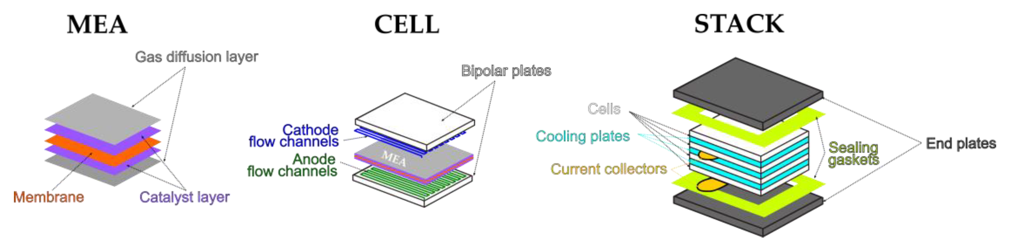
2. Open-Cathode PEM Fuel Cells

A water management system is generally needed in a fuel cell to achieve a fully hydrated membrane while avoiding flooding. The control of hydration is traditionally performed with an external humidification system but can also be achieved by means of self-humidifying methods where the water generated from the reaction, Equation (1), is used to keep the desired level of hydration in the membrane. This solution is preferred in the aviation field because it reduces cost, weight, and complexity [54].

The typical configuration of a self-humidified OCPEMFC for UAV is shown in Figure 3 inclusive of the stack and the BOP. The BOP includes the hydrogen circuit, air path, electric circuit, and controller.

The hydrogen is supplied from a tank that can be of three types: pressurized vessels, cryogenic tanks, or metal-hydride storage systems [41].

The flow rate and the pressure of hydrogen are controlled using a regulation valve. The cathode is dead-end with a purge valve opened with a certain frequency to eliminate water and impurities. As explained in the introduction, the opening of the purge valve determines an outflow of hydrogen.

An inflow of air is guaranteed by the usage of one or more fans and is necessary both for providing the oxidant and as a cooling medium. The motor receives power from the stack or a battery (in particular during the start-up process). The temperature of the stack is regulated by controlling the speed of the fan motors and, therefore, the mass flow rate of the fan.

Since the voltage of the stack decreases with increasing current (i.e., load), a DC/DC converter is used to obtain the desired voltage of the electric load.

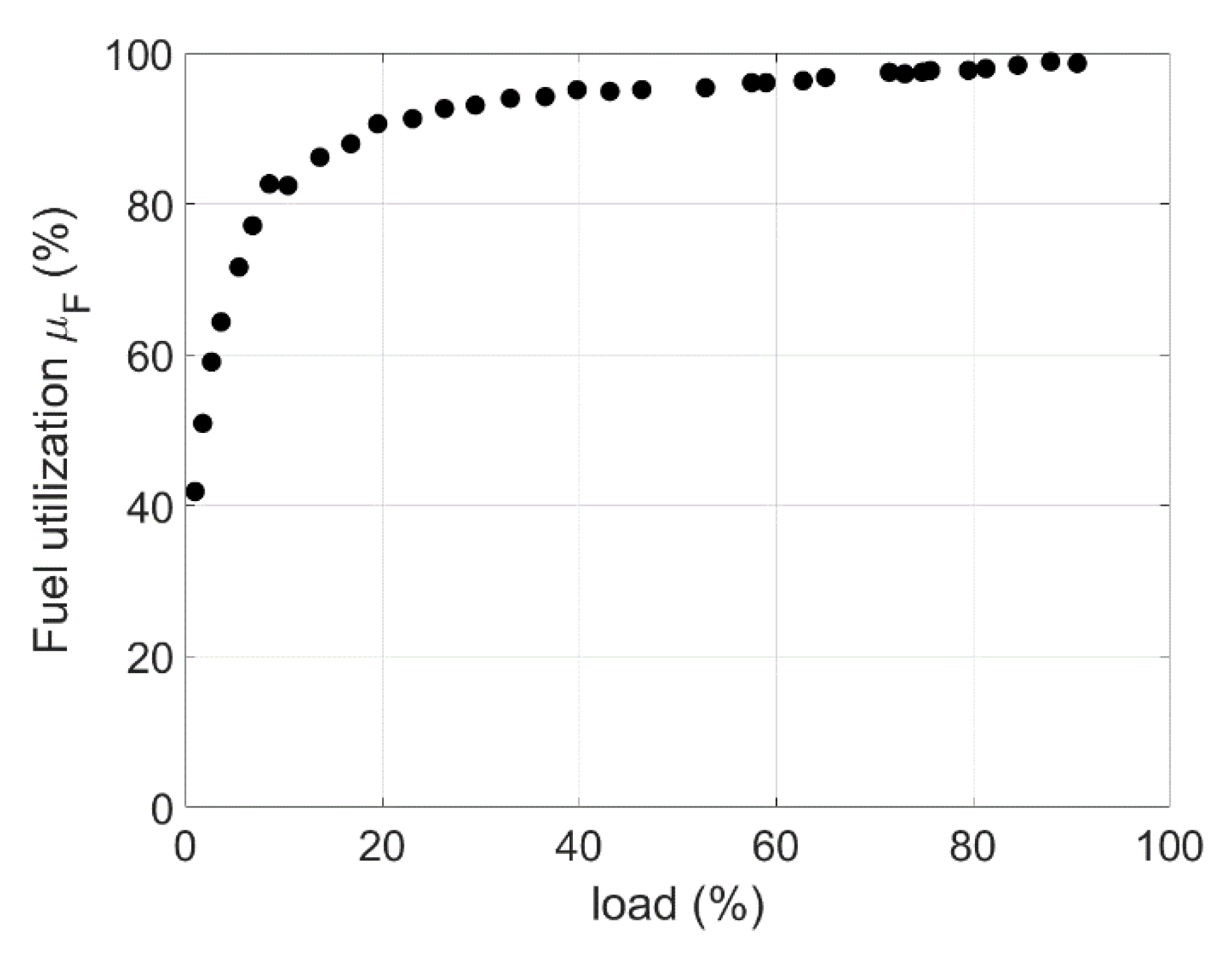
2.1. Performance and Efficiency Indexes

The gross electric power of a stack is given by:

$$P_{el}=V_{st}{I}_{st}$$

(2)

where $V_{st}$ and $I_{st}$ are the voltage and the current of the stack, consisting of $N$ elementary cells in series. Note that $V_{st}$ is a nonlinear function of $I_{st}$ because of a series of phenomena explained later in the paper. Therefore, the net electric power is also a nonlinear function of $I_{st}$. In fact, the main goal of a fuel cell stack model is to predict the dependence of $V_{st}$ and $I_{st}$, the so-called “polarization curve” or “voltage–current curve” that is also affected by operating variables like temperature, pressure, and water content [55].

When the OCPEMFC is analyzed at a system level, it is necessary to encompass the parasitic power of the BOP [56]. The net power of a fuel cell system is given by:

$$P_{net}=V_{st}{I}_{st}{\eta }_{DC-DC}-P_{aux}$$

(3)

where $P_{aux}$ and ${\eta }_{DC-DC}$ are the parasitic power of the auxiliaries and the efficiency of the DC/DC converter, respectively. In an OCPEMFC, the main contribution to $P_{aux}$ is represented by the power of the fan. In [57], for a Horizon H-500 fuel cell, the power consumption of the auxiliary component was found to be dependent on the stack temperature and ranging from 36.5 W at 296.15 K to 52 W at 338.15 K. The auxiliary power consumption of a 100 W OCPEMFC was determined experimentally in [17] and was found to be strongly dependent on the fan voltage control law because of the strong effect of temperature. With appropriate fan speed control, the efficiency was found to increase from 28% to 36%. In [58], a parasitic power of up to 5 W is measured for an H-12 horizon fuel cell with a rated power of 12 W.

The efficiency of the stack can be expressed as:

$${\eta }_{stack}={\mu }_F\frac{V_{st}}{N·E_0}$$

(4)

where ${\mu }_F$ is the fuel utilization rate [55] assumed equal to 0.95 in [59] and 0.9 in [60], while $E_0$ is the electric counterpart of the heating value of hydrogen. It is equal to 1.462 V if the higher heating value (HHV) of hydrogen is considered [60] and 1.254 V for the lower heating value [55]. In a dead-end anode, the fuel utilization rate is affected by the purging process. Purging must not be performed too often to minimize hydrogen loss and membrane drying. In [61], the purging is said to take place when the voltage across the last cell in the stack is less than 0.8 V so that the purge frequency is increased with the load. The purging process causes spikes in the stack voltage [30,62] and in the consumption of hydrogen [20]. In [63], the purging action was found to increase the total fuel consumption by 32% over a driving cycle of 250 s. The purging frequency tends to increase with the nominal power of the stack. The purging valve is activated every 30 s in the H-100 fuel cell stack [30] and 10 s in [64,65] for the H-1000 Horizon fuel cell. Optimization of the purging frequency is performed in [66,67].

The purging process determines a reduction in fuel utilization, particularly at low loads. To quantify this effect, the flow rate of hydrogen without purging was estimated by Verstraete et al. [62] by taking a moving average of the measured data. The fuel utilization curve of Figure 4 was obtained.

The voltage of the fuel cell, $V_{cell}$, is significantly inferior to $E_0$ because of activation, ohmic, and concentration [5] losses that will be described in Section 3.

The net efficiency of a fuel cell system can be expressed as [1]:

$${\eta }_{net}=\frac{P_{net}}{{\dot{m}}_{H_2}HHV}$$

(5)

where ${\dot{m}}_{H_2}$ is the hydrogen mass flow rate and $HHV$ is the higher heating value of $H_2$.

The net system efficiency was found to range between 32% and 49% in the power range of the H-500XP stack [57]. Typical curves of cell voltage, net efficiency, and net power vs. current are reported in Figure 5. Note that the net efficiency, unlike the gross efficiency (which follows the same trend as the cell voltage), tends to zero at low loads and is lower than the gross efficiency because it is affected by the duty cycle of the fan and by the loss of hydrogen caused by the purging action [17]. This evidences the importance of accounting for the parasitic power of the fan and the other components of the BOP.

Note that the maximum efficiency (red star in Figure 5) is obtained at low loads and high voltages while the maximum power (blue star in Figure 5) is obtained at medium-high currents and low voltages. According to the field of application, FC system designers can select the voltage that maximizes power, efficiency, or fuel utilization [68].

The performance of an OCPEMFC system can be measured also in terms of stack cooling effectiveness $\epsilon$ [69]:

$$\epsilon ={\dot{m}}_{air}{c}_{p,air}(T_{st}-T_{amb})/{\dot{\mathrm{Q}}}_{gen}$$

(6)

where $T_{st}$ and $T_{amb}$ are the temperatures of the stack and the ambient, respectively. The numerator of Equation (6) is the heat removal rate of the cooling system while ${\dot{\mathrm{Q}}}_{gen}$ is the thermal power generated by the stack.

A cooling device can be also characterized in terms of the ratio between heat removal rate and parasitic power. A well-designed cooling system can achieve an effectiveness ratio between 20% and 40%.

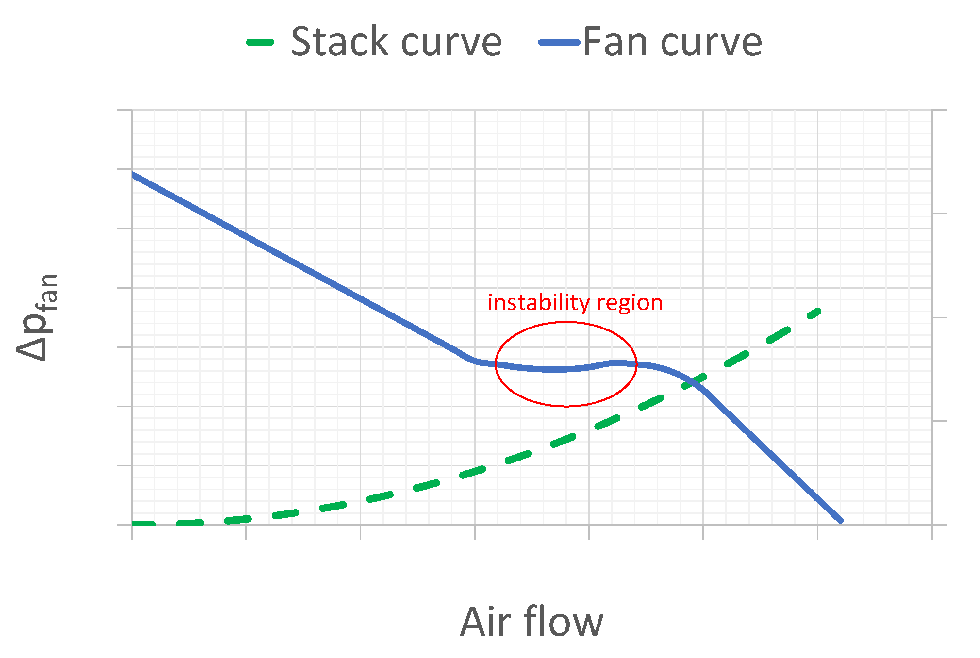
2.2. Fan Working Point and Speed Control

In OCPEMFCs, the role of the fan is to direct the airflow rate toward the air channels of the cathode and to overcome the major and minor head losses [70,71] of the stack.

The pressure of the air supplied to the cathode is the sum of the ambient pressure and the rise in pressure generated by the fan. The performance of a fan is expressed by its performance or characteristic curve that reports the pressure head vs. the air flow ratio. The pressure head in this application is given by:

$$∆p_{fan}=p_c-p_{amb}$$

(7)

where $p_c$ is the cathode pressure.

An example of the performance curve of the fan is reported in Figure 6 together with a hypothetical stack resistance curve. The fan curve refers to the Delta FFB-0912-EHE model used in the Horizon H-1000 stack [64]. The actual air mass flow rate is obtained by intersecting the fan curve with the stack resistance curve [8], which is a quadratic function of the air flow rate. In general, the pressure head decreases when the air mass flow increases. However, most fans have a region of the performance curve where the pressure head increases with ${\dot{m}}_{air}$ like the stack resistance curve (the instability region of Figure 6). This region is to be avoided because the fan presents unstable behavior (stall). If the fan attempts to generate more airflow, the system pressure increases, reducing the generated airflow. As airflow decreases, the system pressure also decreases, and the fan responds by generating more airflow. This induces larger changes in flow rates, which in turn can lead to cyclic behavior of the air flow rate.

The fan must be selected so that its operating point falls in the stable part of the characteristic to guarantee a stable operation and avoid poor fan efficiency and wear on the fan components [72].

Centrifugal or axial fans can be adopted according to the desired air velocity, and two or more fans can be connected or in series to change the operating point. A comparison of centrifugal and axial fans with the different rated speeds is performed in [72]. However, the working point is affected slightly by the cell voltage and strongly by the fan speed.

A variable rotation speed allows the cooling air flow rate to be adjusted to regulate the stack temperature, reducing the noise of the fan and saving energy when full speed is not required. There are two main ways to control the speed of the fan: variable DC voltage supply and PWM (pulse-width modulation). In the first case, a series resistor is used to cause a voltage drop in the supply wire. The lower bound of voltage is limited by the need to avoid a stall in the fan. In the second and most common case, the speed of the fan is determined by the width of the PWM duty cycle while the input voltage is constant. A duty cycle of 40% keeps the electric motor on for 40% of the total time of the PWM signal, and the other 60% of the time, it will remain off. PWM is preferred because it does not generate additional heat, reduces noise thanks to the high-frequency driving signal, and increases the operational speed bandwidth [73]. With this technique, the speed variation of cooling fans is within 30–100% of the rated speed and the minimum speed achieved with PWM controllers is much lower than with DC fans. The duty cycle D is expressed as the ratio between the duration of pulse width and the period of the signal cycle. The fan speed response is almost linear with the PWM duty cycle in the operational bandwidth (D > 30%) [73].

2.3. Testing Procedure and Facilities

The characterization of a fuel cell system can address different aspects [1,5]:

• Overall performance (I–V curve, net power curve);
• Relative effect of the three main loss mechanisms;
• Mass transport proprieties;
• Parasitic losses;
• Structure of catalyst, electrodes and flows;
• Heat balance;
• Lifetime issues;

According to [1], the most useful methods for electrochemical characterizations of the stack are current–voltage measurements, current interrupt tests, electrochemical impedance spectroscopy, and cyclic voltammetry.

Current–voltage measurements are usually performed with galvanostatic techniques where the current is controlled by the user and the resulting voltage is recorded. In the first case, the current is gradually scanned in time from zero to the maximum value, and the voltage is measured after a long relaxation time. As pointed out in [1], it is important to ensure that steady-state conditions are reached. Moreover, test conditions must be carefully controlled and documented. To address the first point, it is necessary to conduct a series of measurements at different speeds. For the second point, a warm-up must be performed by operating the cell at a fixed current load for 30–60 min before testing and recording the fuel cell temperatures of the gases and of the stack during the measurements. The pressure at the inlets and outlets and the flows of reactants and products must be also recorded.

In the current interrupt measurement, a current is abruptly imposed or withdrawn, and the time signal of voltage is measured until it approaches the steady stage value. This method is used in [63] to tune a dynamic model of the fuel cell stack.

In electrochemical impedance spectroscopy, a sinusoidal perturbation is applied to the system and the amplitude and phase shifts of the resulting signal are measured. By repeating the test over a wide range of frequencies, an impedance spectrum is obtained. The difference between the low-frequency intercept and the high-frequency intercept of the real axis of an impedance spectrum represents the resistance of the electrode processes while the high-frequency intercept is the ohmic resistance [35].

Regarding the relative effect of losses in a stack, O’Hayre et al. [4] explain how it is possible to separate the individual contributions of activation, ohmic, and concentration losses from a current–voltage curve. As for the relative effect of the three loss mechanisms, from the results reported in [68,74], the most relevant contribution is that associated with activation losses.

The test bench of whole OCPEMFC systems usually consists of data acquisition systems, controllers for the fan voltage and the purging time, thermocouples for temperature measurement, and a flow-rate measurement for hydrogen flow rate [14,37]. A programmable electronic load is used to reproduce a variable current load. Generally, tests are performed in rooms where the temperature and humidity are not controlled, and their values are sometimes not even recorded. However, the details of pressure, temperature, humidity, and relaxation times are rarely reported in the scientific literature.

Altitude chambers have been proposed to reproduce the operation of a fuel cell system at high (<11,000 m) and very high altitudes (>11,000 m). Often, these chambers allow the control of pressure while humidity and temperature can be monitored. An environmental test chamber was included in a wind tunnel by Atkinson et al. [35] to study the effect of altitude on a single cell. The test system adopted in [35] includes a frequency response analyzer for the analysis of the impedance spectrum. Saadi et al. [26] used electrochemical impendence spectroscopy (EIS) to investigate the phenomena of diffusion and charge transfer. Wind tunnels are employed in [18] to study edge cooling in a UAV and in [75] to measure the convective heat transfer coefficient of a PEM. In [30], the stack is tested in an environmental chamber that allows the control of humidity, temperature, and oxygen concentration.

2.4. Transient Phenomena in an OCPEMFC

In applications characterized by rapid variation of loads like UAVs, the analysis of the dynamic behavior of PEMFCs is of the utmost importance [55,76]. One of the limitations of fuel cells compared with batteries and supercapacitors is the slower response to variable load profiles like that reported in Figure 2. A transient of 20–30 s from no load to rated power was measured in [60] for a fuel cell. In [61], the dynamic responses to step-down (20 A–0 A) and step-up (0 A–20 A) transient loads of a 1.2 kW Ballard fuel cell and a lithium battery were found to be 1.2 s and 0.6 s, respectively. This explains the need for the fuel cell to be coupled with a battery or a supercapacitor to improve the response to fast load changes [77]. Analyzing the transient behavior of a PEMFC is also significant in the case of start-up and shut-down operations to achieve a rapid increase in the stack temperature and to avoid the degradation of the fuel cell, respectively [78].

Different interconnected dynamics processes take place in an OCPEMFC, each requiring a suitable control action to optimize the behavior of the whole system [55,78].

The control of the temperature is the most critical issue in an OCPEMFC and is achieved by acting on the speed of the fan. On the one hand, an increase in temperature accelerates the electrochemical reaction and improves the efficiency. On the other hand, a too-high temperature can damage the membrane and increase the internal resistance [79]. Moreover, high temperatures cause dehydration in the catalyst layer and reduce the cell voltage [30]. As a consequence, both performance and efficiency are degraded. The optimal temperature of the stack according to Abul-Hawa et al. [55] should be 80 °C while a range of 65–85 °C is considered in [79]. In other investigations, the reference value for temperature is varied with the load [80]. Under cold-start operation, heaters are used for a fast warm-up of the stack [37].

To avoid an excessive difference in pressure across the membrane that can damage the membrane and increase reactant crossover, it is necessary to regulate the feeding pressure of hydrogen, especially at high-altitude, where the cathode pressure is lower [55].

The humidity of the cathode air must be high to minimize the internal resistance of the fuel cell but not too high to avoid flooding. Sudden variations in the water content cause hysteresis in the dynamic polarization curve [62]. In particular, a lower voltage at a given current is obtained in the case of load reduction. The faster the load variation, the higher the degree of hysteresis. The water content in the membrane is controlled with an external circuit humidification circuit. In self-humidifying fuel cells [81], additives are adopted into the catalyst layer or in the membrane to retain the water generated by reaction (1).

During transients, it is also important to avoid starvation of reactants to preserve the performances [79,82]. Using more fuel than needed for a specified power (i.e., adopting low values of ${\mu }_F$) is a possibility, but this determines a waste of hydrogen, which is a precious energy carrier. In [79], the optimization of stack orientation is also suggested as a way to solve the problem of oxygen starvation.

At a cell level, a further dynamic phenomenon has to be considered: the double-layer capacitor effect, which happens during the regular operation of the cell and is caused by the accumulation of charge at the anode–electrolyte and electrolyte–cathode layers. However, the double-layer capacitor effect has a much smaller time constant compared with the other dynamic phenomena, as shown in

Table 1. Time constants of the transient phenomena in open-cathode fuel cells.

Phenomenon	Scale of Time Constants	Source
Stack temperature	$100 \mathrm{s}$	[55]
Membrane hydration	$10 \mathrm{s}$	[83]
Fan speed	$1 \mathrm{s}$	[30]
Gas transport	$\text{0.01–0.1} \mathrm{s}$	[55]
Double layer discharge	$0.1 \mathsf{\mu }\mathrm{s}$	[83]

.

The orders of magnitude of the time constants for membrane hydration and electrochemical double-layer were estimated numerically in [83] and confirmed experimentally in [62].

2.5. Control Methods

A detailed review of control methods applied to OCPEMFCs is beyond the goal of this investigation. Nevertheless, it is significant to describe the control approaches for two reasons. On the one hand, the dynamic behavior of the fuel cell is strictly related to the control actions performed on the system. On the other hand, the number of recent papers on advanced control techniques underlines the importance of making available accurate and comprehensive control-oriented models.

In an open-cathode configuration, the main control action is related to temperature and is achieved by regulating a single component, i.e., the fan [47]. This makes the air stoichiometry rate calculation more critical than in a closed-cathode fuel cell [84]. On the other hand, Ou et al. [47] pointed out that if the focus of the control is only on the temperature, oxygen starvation can happen, in particular when a low air flow is required for cooling, for example, when the fuel cell has not yet reached the optimal temperature after the start from ambient conditions. To solve this problem, Ou et al. proposed a double calculation of the excess air to avoid overheating and protect the cell from air starvation.

In [30], two dynamic states are considered: the stack temperature and the liquid water saturation. The load current and the cathode inlet air temperature are the measurable external perturbations. The control variable is the inlet air velocity through the PWM control of the fan. The output of the system is the voltage. In this investigation, a local PI controller is used to regulate the voltage of the cooling fan, and an extremum-seeking algorithm is applied to obtain the optimal temperature set point for the PI controller. However, the experimental validation revealed that this controller was not able to stabilize the voltage because of the slow system dynamics of the drying of the catalyst layer. For this reason, other controllers were proposed in a subsequent study by Strahl et al. [85]. A review of the control method for temperature can be found in [14], where three control parameters are considered: the duty cycle of the fan, the cycle time, and the difference between the average output power of the current cycle and the previous cycle.

In [47], the control objective is to maximize the net power output and prevent overheating. For this scope, the relationship between net power and the duty cycle is mapped for different load currents, and the optimal value of the fan duty ratio is obtained. Then, the same process is used to identify the minimum duty ratio that allows the fuel cell to operate in safe temperature conditions. They found that the oxygen excess ratio of power optimization requires more air flow mass than the cooling system at high loads, and at lower currents, temperature protection is more critical. The oxygen excess ratio was selected as the maximum between the value that minimizes the net power and the minimum value required to avoid overheating. The values of the optimal oxygen excess ratios were fitted using a third-degree polynomial function and used as a reference for the fan control performed with a conventional PI controller.

The classical PI or PID controller with feedback is often used for the control of OCPEMFC, but sliding mode control has recently been proposed ([82,86]) to ensure the desired value of the oxygen excess ratio. A PID controller is a simple, economical, and easy-to-implement solution for single-input–single-output systems and is therefore applied in a variety of applications including the control of a fuel cell system [87]. The method is based on the difference (error) between a measured process variable and its setpoint and applies a correction based on the proportional, integral, and derivative terms. This control method requires tuning to find the best values of the constants used in the three terms. The tuning of the PID is addressed in detail in [65], where the author identified the best setting in terms of a trade-off between fast response and reactants consumption. In the work of Strahl et al. [30] on an H-100 stack, the proportional gain of the PID is 0.8, and the integrator time constant is 20.

A review of control methods used in fuel cell systems to avoid starvation can be found in [79]. They underlined the drawbacks of classical proportional integral and derivative controllers, i.e., the inaccuracy and slow response time that can be solved by more advanced controllers like the sliding mode, adaptive, neural network, fuzzy logic [88], and model-predictive controllers. In the last case, the availability of a fast but accurate dynamic model of the fuel cell system is critical. In [89], a model predictive control (MPC) and a PID controller were designed to control the voltage at the desired value by regulating both hydrogen and air flow rates. The two controllers were compared under different operating conditions and the MPC was found to be superior in fulfilling the stabilization of the voltage. Similarly, a comparison between MPC and traditional PID is reported in [90]. Li et al. [91] developed an active disturbance rejection controller (ADRC) with a switching law for temperature regulation.

In [74], fuzzy logic is used for the control of the temperature using the temperature error, its derivative, and current as inputs and the duty cycle of the fan as an output. A constant temperature of 35 °C was set as a reference. In [88], both temperature and humidity are controlled by employing a fuzzy-based logic that controls the PWM signal of the fan and the behavior of the external humidifier. The goal of the investigation presented in [92] was the simultaneous control of current and temperature to supply the requested power with the highest possible efficiency, i.e., with the lowest consumption of hydrogen. A fuzzy logic controller (FLC) is used to reach the reference temperature (that depends on the current) while a PI controller is used to control the current. As discussed in [92], PID controllers cause large temperature overshoots because they work well for a limited operating range. Moreover, their tuning is dependent on the accuracy of the model. On the other hand, FLCs are more flexible in terms of range of operation and also work well with not very accurate models.

In most of the papers cited above, the reference temperature is assumed to be constant (see, for example, [88]) while in [80], the optimal reference temperature is expressed as a function of the current. The results reported in [30] show that, for each current, there is an optimal stack temperature and, therefore, a different PWM value. Moreover, the optimal values of the temperature in that investigation were found to be higher than the default values considered in the standard controller. This also allows a reduction in the parasitic power of the fan thanks to the lower PWM. In [14], a temperature reference-seeking algorithm is employed to determine the optimal operating temperature in variable environmental conditions. The author of this review believes this approach to be particularly suitable for aerospace applications, but a further step is required. One of the scenarios investigated in [14] is a typical mission of a UAV. However, the effect of different values of ambient pressure and temperature due to flight altitude is not considered. Their strategy allowed an increase of up to 2.78% of the net power compared with the constant duty cycle control.

To optimize the behavior of the fuel cell system, it is also possible to control the operating point of the fuel cell to ensure maximum power or maximum efficiency through the power management unit that has the role of matching the operating point of the fuel cell with the load demand, i.e., to ensure that the power generated by the stack is equal to the power requested by the load [55]. Power management is needed because the voltage produced by the stack decreases when the current increases. The unstable direct current generated from the stack has to be strictly controlled to ensure the rapid delivery of the load required during fast transients [79]. A DC/DC power converter needs to be introduced between the fuel cell and the load to convert and stabilize the bus voltage [1]. An excessive change in DC/DC input current generates an insufficient supply of air. Therefore, the topology and control of the DC/DC converters must be designed and optimized in combination with the PEMFC system to improve output performances. To solve this problem, Zhao et al. [33] propose a PEMFC dynamic model that considers the disturbances of the internal load, the centrifugal compressor with its driving motors, and the external UAV power load under variable elevations and operating conditions.

Another possibility to control voltage is through hybridization. As already stated, the response of a fuel cell system to changes in demand is not comparable to that of its competitor (i.e., internal combustion engines and batteries) because its response to transient changes in load depends on the management of heat and water content, regulation of pressure and flow rate of the reactants [55]. For this reason, a secondary energy storage device (battery or capacitor) is needed to support the fuel cell during transients. Verstraete et al. [62] found that the controller developed by Horizon Energy Systems for their self-humidified stacks short circuits the stack output power every 10 s to increase the efficiency. A supercapacitor and/or a battery is needed to ensure continuous power during the short-circuiting process. In [77], a controller is developed for a fuel cell/supercapacitor system to keep the fuel cell power between the desired bounds and to limit the variation slope of the fuel cell to avoid starvation. Hybrid systems with batteries or supercapacitors can be passive or active [46]. In a passive system, no DC/DC converter is used; therefore, the voltage of the two systems (the fuel cell and the secondary storage system) must be similar. This reduces the weight and complexity but does not allow operation flexibility. A review of hybrid electric configurations with fuel cells for UAV applications can be found in [93].

2.6. Effect of Altitude and Cold Start

The variation in ambient temperature, pressure, and relative humidity with elevation can degrade the fuel cell performances and make the thermal management of the fuel cell system [94] more difficult. In fact, the request of air velocity and volumetric flow rate for the cooling of the fuel cell [75] increases with altitude because of the lower density. Since the increase in air velocity is smaller than the density variation, the Reynolds number of the flow also decreases.

The impact of vibration, cathode air starvation, low pressure, and cold start on PEMSs utilized in high-altitude environments is addressed in [95]. As the altitude rises, the drop in temperature and pressure and cathode air starvation cause a decline in the cell performance due to damage to the membrane electrode assembly. The effect of low pressure can be overcome by increasing the cathode air flow rate, but it is necessary to monitor the membrane humidity. A critical value of the air stoichiometric ratio must not be reached to prevent the membrane from drying.

Altitude affects the behavior of both closed-cathode and open-cathode fuel cells [67]. The effect of altitude on voltage and power in OCPEMFCs was experimentally evaluated for a single-cell system [35]. The fuel cell was tested in a depressurized chamber to simulate the pressure up to 3239 m and a decrease of 17% was found in the cell power. This reduction is suggested to be due to higher activation losses due to the operation at lower oxygen partial pressure. Moreover, the ohmic resistance increases because of the low cell temperature and relative humidity. On the other hand, the cell can dissipate waste heat more effectively at high altitudes thanks to the lower ambient temperature. Therefore, the maximum current density of the cell increases. However, as pointed out in [35], it is not possible to associate such variation only to altitude because the fuel cell is highly sensitive to ambient relative humidity and temperature.

The authors of [35] also pointed out how the availability of cool air at high temperatures could enable the removal of many traditional BOP components. The implementation of the open-cathode flexible fuel cell to cover the airframe is suggested for UAVs while hollow structures like the wings of fuselage can be used for hydrogen storage. On the other hand, this solution does not allow control of the fuel cell stack and, therefore, can cause the degradation of the cell performance when the temperature. They found that the forced airflow has little influence on OCPEMFC performance at low and intermediate cell voltage (<0.65 V).

When the stack works at an ambient temperature under 0 °C, the water produced by the reaction can solidify and the increase in water volume can destroy the MEA. To avoid such a problem, it is necessary to ensure that the heating rate is more rapid than the freezing rate of water by employing shutdown purging, external heating, etc. [69,95].

3. General Models for Fuel Cell Stack

As pointed out in [55], the stack is described by three sets of variables: geometrical, operational, and performance. The effect of technological and geometrical parameters on the behavior of the stack can be addressed using white models like computational fluid dynamic (CFD) methods. As explained in the introduction, this class of models is not included in this review because it cannot be applied to a system-level simulation. On the other hand, operational variables like the pressure, control of reactants, stack temperature, and water content can be addressed with grey or semi-empirical approaches.

The main goal of these models is to approximate the “voltage–current” or “polarization curve” of the fuel cell that presents the typical trend shown in Figure 7 with the red line. It is important to notice that, from an electrochemical point of view, the polarization curve can be reported in terms of cell voltage vs. current density or stack voltage vs. current. The first approach is employed when the focus is on the single cell [1]. At the stack level, instead, it is the indifferent to represent the polarization curve in terms of current ($I_{st}$) or current density ($i=\frac{I_{st}}{S_{act}}$).

All models proposed in the scientific literature treat hydrogen and air as ideal gases, a hypothesis justified by the low working temperature of PEM fuel cells.

The semi-empiric models adopted to analyze the behavior of the stack in OCPEMFCs and CCPEMFCs are the same because the two systems differ only for the BOP. A detailed analysis of static and dynamic models for the stack of CCPEMFCs can be found in [24]. Here, a summary is reported.

Theoretically, a single cell can generate an open-circuit reversible voltage $E_0$ given by [5,96]:

$$E_0=1.229-8.46\times {10}^{-4}\left(T_{st}-298.15\right)$$

(8)

where $T_{st}$ is the stack temperature.

The first term, 1.229 V, is obtained from the Gibbs free energy change at 298 K and 1 atm of Equation (1) and represents the highest voltage obtainable from a hydrogen–oxygen fuel cell. Under non-standard conditions, the open-circuit voltage, called Nernst voltage, $E_{Nernst}$, can be calculated as follows:

$$E_{Nernst}=E_0+\frac{R{T}_{st}}{2F}\left[\ln \left(p_{H_2}\right)+\frac{1}{2}\ln \left(p_{O_2}\right)\right]$$

(9)

where $R$ and $F$ are the ideal gas constant and the Faraday constant, respectively, and $p_{H_2}$ and $p_{O_2}$ are the partial pressures of the reactants. The partial pressure of the water does not contribute at temperatures below 100 °C, being in a liquid state. The partial pressure of hydrogen depends on the hydrogen feeding pressure. In an OCPEMFC, the partial pressure of oxygen depends on the molar fraction of oxygen in the atmospheric air. In the case of dry air at sea level, it is about 0.21 atm [5]. According to the International Standard Atmosphere model (ISA), temperature $T_{amb}$ and pressure $p_{amb}$ at an altitude from sea level up to 11,000 m can be calculated as:

$$T_{amb}\left(h_L\right)=T_0-6.5 h_L$$

(10)

$$p_{amb}\left(h_L\right)=p_0{\left(1-6.5\frac{h_L}{T_0}\right)}^{5.2561}$$

(11)

where $T_0=288.15 \mathrm{K}$ and $p_0=1.013 \mathrm{b}\mathrm{a}\mathrm{r}$ and $h_L$ is the altitude in meters.

The humidity of the air in parts per million by volume (ppmv) can be estimated from 0 to 15 km with the following empirical correlation [96]:

$$H_{2}O\left(ppmv\right)=\frac{\mathrm{16,176}}{1+\exp \left(\frac{h_L}{2299}\right)}+20.51\frac{h_L}{1000}-320$$

(12)

The Nernst voltage is the reversible open circuit of the electrochemical cell associated to the change in Gibbs energy in the reaction (Equation (1)) [5]. Once the fuel cell is subject to an external load, a current is generated and voltage drops because of the irreversibility associate to activation, crossover, ohmic, and mass concentration processes [15] as shown in Figure 7. These losses occur at all currents, but the activation process is more relevant at low currents while the concentration voltage drop is significant only when the current approaches its maximum value.

Neglecting the only dynamic process in the cell, i.e., the double layer charging effect, the cell is modeled with the equivalent circuit of Figure 8 and the voltage of the stack can be calculated as:

$$V_{st}=N\left(E_{Nernst}-∆V_{ohm}-∆V_{act}-∆V_{conc}\right)$$

(13)

The voltage drop ∆V caused by irreversibility is expressed as the sum of ohmic ($∆V_{ohm}$), activation ($∆V_{act}$), and concentration ($∆V_{conc}$) voltage drop.

3.1. Activation Losses

The activation losses are calculated using the Tafel equation or, more recently, with Amphett’s model [97].

The Tafel equation, in the more general form, is:

$$∆V_{act}=\frac{R{T}_{st}}{2\alpha F}ln\left(\frac{I_{st}+I_n}{S_{act}{ I}_0}\right)$$

(14)

This equation is valid only for $I_{st}>I_0$, where ${ I}_0$ is the exchange current, the minimum current at which the voltage drop is observable [5]. The transfer coefficient $\alpha$ measures the part of electrical energy that is utilized in varying the rate of the electrochemical reaction. $I_n$, sometimes neglected, takes into account fuel crossover and internal currents, i.e., fuels and electrons that move through the electrolyte. The values of the parameters in this equation are assumed equal to $\alpha =0.2571$, $I_n/S_{act}=0.00037707 A/\mathrm{c}{\mathrm{m}}^2$ and $I_0=0.0047758 A/\mathrm{c}{\mathrm{m}}^2$ in [8] for a OCPEMFC with a nominal power of 500 W. However, the transfer coefficient $\alpha$ is affected by temperature [96] and oxygen partial pressure [30]. For more details, please refer to [24].

The exchange current increases exponentially with temperature:

$$\frac{{ I}_0}{S_{act}}=1.256-8\exp [0.10988(T_{st}-323.15)]$$

(15)

In Amphett’s model, the activation losses are accounted for with the following equation:

$$∆V_{act}={\xi }_1+{\xi }_2{T}_{st}+{\xi }_3{T}_{st}\ln \left(c_{O_2}\right)+{\xi }_4{T}_{st}\ln \left(I_{st}\right)$$

(16)

where ${\xi }_i$ with i = 1, 4 are parameters that originally had a physical interpretation but are usually regarded as parameters to be tuned. The values proposed in the scientific literature for these parameters are summarized in

Table 2. Values of the empirical parameters of Equation (16) found in the scientific literature.

Stack Name	${\mathit{\xi }}_1$	${\mathit{\xi }}_2$	${\mathit{\xi }}_3$	${\mathit{\xi }}_4$	Ref.
Horizon 2000 W	$-0.9477$	$0.0033$	$7.5\times {10}^{-5}$	$-1.915\times {10}^{-4}$	[69,88]
Horizon 1000 W	−0.944	3.54 × 10−3	$8\times {10}^{-5}$	$-1.96\times {10}^{-4}$	[65]
Horizon 500 W	$-1.0$	$0.0034$	$7.8\times {10}^{-5}$	$-1.85\times {10}^{-4}$	[57]
500 W	$-1.29$	$0.0032$	$2.6\times {10}^{-5}$	$-1.5\times {10}^{-4}$	[92]
Ballard Mark V FC 5 kW	$-0.948$	From Equation (17)	$7.6\times {10}^{-5}$	$-1.93\times {10}^{-4}$	[87]
Ballard Mark V FC 5 kW	$-0.948$	0.00312	$7.6\times {10}^{-5}$	$-1.93\times {10}^{-4}$	[98]
Ballard Mark IV FC	$-0.9514$	0.00312	$7.4\times {10}^{-5}$	$-1.87\times {10}^{-4}$	[99]
Ballard Mark V FC	$-0.944$	0.00354	$7.8\times {10}^{-5}$	$-1.96\times {10}^{-4}$	[99]
NedStack PS6 (500 W)	−1.023071	3.4760 × 10−3	7.7883 × 10−5	$-0.954\times {10}^{-4}$	[91]
NedStack PS6 (500 W)	−1.1997	3.4172 × 10−3 3.5505 × 10−3	3.66 × 10−5 4.614 × 10−5	$-0.954\times {10}^{-4}$	[100]
Not declared	−0.944	3.54 × 10−3	$7.8\times {10}^{-5}$	$-1.96\times {10}^{-4}$	[55]
Unspecified 300 W stack	$-0.948$	From Equation (17)	$7.6\times {10}^{-5}$	$-1.93\times {10}^{-4}$	[94]

.

As shown by Qinshan [68], small variations in the parameters generate large variations in the polarization curve.

In [87,94], the second coefficient is computed as proposed by the authors of [99] in an attempt to generalize the model:

$${\xi }_2=0.00286+0.002\ln \left(S_{act}\right)+4.3·{10}^{-5}+\ln c_{H2}$$

(17)

where $c_{H2}$ is the hydrogen concentration, which depends on stack temperature and hydrogen pressure, $P_{H_2}$:

$$c_{H_2}=9{.17·{10}^{-7}P}_{H_2}\exp \left(-\frac{77}{T_{st}}\right)$$

(18)

An increase from $p_1$ to $p_2$ in the pressure determines a gain in the cell voltage that can be estimated as [5]:

$$∆V_{gain}=c·\ln \left(\frac{p_2}{p_1}\right)$$

(19)

where $c$ is a function of exchange current density and is influenced by pressure, humidity, and fuel cell design [5].

3.2. Ohmic Losses

Ohmic losses are modeled with the equivalent resistance $R_{ohm}$:

$$∆V_{ohm}=R_{ohm}{I}_{st}$$

(20)

The ohmic resistance incorporates the resistance encountered by the ions in the passage through the membrane, $R_{mem}$, and the contact resistance, $R_c$, between cells [80]. $R_{mem}$ depends on the membrane thickness $t_m$, the water content of the membrane ${ \lambda }_m$, the stack temperature ${ T}_{st}$, and the current density [69,90,94]:

$$R_{mem}=\frac{181.6t_m·\left[1-0.03\frac{{ I}_{St}}{S_{act}}+0.062{\left(\frac{{ T}_{st}}{303}\right)}^2{\left(\frac{{ I}_{St}}{S_{act}}\right)}^{2.5} \right]}{\left[{\lambda }_m-0.634-3\frac{{ I}_{St}}{S_{act}}\right]·S_{act}·\exp \left(4.18\frac{T_{st}-303}{T_s}\right)}$$

(21)

Recently, an empirical model has been proposed by Kandidayeni [36] to address the dependence of ohmic resistance on stack temperature and current density:

$$R_{ohm}={\zeta }_1+{\zeta }_2{T}_{st}+{\zeta }_3\frac{I_{st}}{S_{act}}$$

(22)

where ${\zeta }_1,{\zeta }_2$ and ${\zeta }_3$ are empirical parameters.

The internal resistance is also affected by stack pressure [5], but this effect is not addressed in the scientific literature, to the author’s knowledge.

3.3. Concentration Losses

Concentration losses are relevant only in the high-current region [5]. Since the fuel cell is normally operated between the max efficiency load and the maximum power, they are often neglected.

The loss of voltage caused by mass transport is generally modeled with the exponential equation reported in Equation (23); see, for example, [87].

$$∆V_{conc}=\mathrm{B\; ln}\left(1-\frac{I_{st}}{I_{max}}\right)$$

(23)

where B is assumed equal to $\frac{R{T}_{st}}{2F}$ in [42,80,92] but can be expressed as function of current, temperature, and/or other parameters [24].

An empirical exponential model is used as an alternative to Equation (23):

$$∆V_{conc}=m·\exp \left(N{I}_{st}\right)+b·\ln \left(\frac{P_{O_2}}{a}\right)$$

(24)

where $m$, $b$, and $a$ are empirical coefficients.

3.4. Simplified Parametric Models

The equations reported in the previous sub-sections need detailed information about the stacks. In the absence of such information, fully parametric models were proposed in the scientific literature. The most common is the equation proposed by Larminie and Dicks [5] to account for all losses:

$$V=E_0-A ·ln\left(i\right)-R_i·i-m·exp\left(ni\right)$$

(25)

The values of the tuning parameters $E_0$, $A$, $R_i$, $m$, and $n$ for two different stacks are reported in

Table 3. Fitting of the simplified parametric model.

Stack	${\mathit{E}}_0$	$\mathit{A} \left(\mathit{V}\mathit{l}\mathit{n}{\mathit{A}}^{-1}\right)$	${\mathit{R}}_{\mathit{i}} \left(\mathsf{\Omega }\right)$	$\mathit{m} \left(\mathit{V}\right)$	$\mathit{n}\left({\mathit{A}}^{-1}\right)$	Ref.
Horizon H-1000	$59.99$	$0.07559$	$0.24493$	$0.2$	$0.003$	[63]
Aerostack 300 W	$30.48$	$0.4947$	$0.5002$	$1.972\times {10}^{-4}$	$0.5002$	[62]

to underline their large variability. In the first case, ref. [63], the fitting of the model is performed by using a least squares system identification technique while an online identification approach is used in [62] for the 300 W Aerostack fuel cell.

To increase the generality of the model by accounting for the effect of feeding pressure, an additional term can be added to Equation (25) [101]:

$$V=E_0-A ·ln\left(i\right)-R_i·i-m·exp\left(ni\right)-C·ln\left(\frac{P}{P_{O_2}}\right)$$

(26)

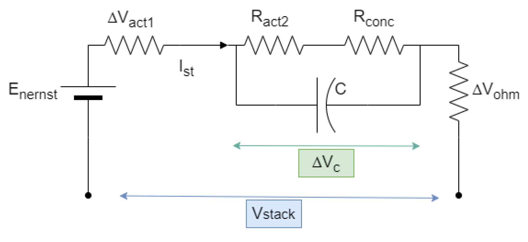
3.5. Double-Layer Capacitor Effect

Under dynamic operation, the generation of two layers charged with opposite polarity in the boundary between the electrodes and the membrane makes the cell act as a capacitor [62] and determines a hysteresis in the voltage–current curve.

This phenomenon is modeled by adding a capacitor in the equivalent electric circuit in Figure 8 in parallel with the activation, the ohmic, and/or the concentration losses. The scheme proposed by [5] and adopted by several studies in the scientific literature is shown in Figure 9. Alternatively, this effect can be addressed by using a time constant.

More details about the modeling of this dynamic process can be found in the previous review paper [24]. Since the time scale of the double-layer effect is much smaller than the other dynamic processes that take place in fuel cells, it can be neglected when analyzing the whole fuel cell system. Therefore, the models described in Section 3 can be used as quasi-static approaches for the dynamic modeling of the whole fuel cell system.

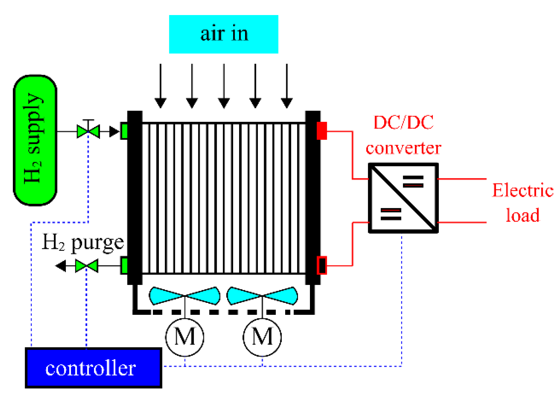
4. Modeling the BOP of an Open-Cathode Fuel Cell

The stack temperature is affected by the load (current) and the current/voltage operating point of the cell is in turn affected by the cell temperature. The coupling between the voltage model and the thermal model is well put into evidence in the scientific literature (see, for example, [36]), but the purging process is also important to have an accurate prediction of the net power and overall efficiency of the system.

For the modeling of an OCPEMFC inclusive of its BOP, the rate of change in reactants is usually addressed with a quasi-static approach while the cooling system, inclusive of the fan speed and stack temperature dynamics, is analyzed by solving dynamic equations.

4.1. Flows of Reactants and Products

Under constant operation conditions, the stoichiometric flow rates of hydrogen ${\dot{m}}_{H_2, react}$, oxygen ${\dot{m}}_{O_2,react}$, and water ${\dot{m}}_{H_{2}O,gen}$ can be expressed as a function of to the stack current [5,55] using the basic reaction of Equation (1):

$${\dot{m}}_{H_2, react}=\frac{M_{H_2}}{2F}·I_{st}$$

(27)

$${\dot{m}}_{O_2,react}=\frac{M_{O_2}}{4F}·I_{st}$$

(28)

where $M_{H_2}$ and $M_{O_2}$ are the molar mass of hydrogen and oxygen, respectively. Oxygen in an OCPEMFC can be obtained only from ambient air, so it is better to express the requirement of oxygen in terms of stochiometric air. To avoid starvation, the air mass flow rate must exceed the stoichiometric value by a factor $\lambda$ named excess ratio. Therefore, the mass flow rate of air is:

$${\dot{m}}_{air}=\lambda \frac{M_{air}}{M_{O_2}2F}·I_{st}$$

(29)

While the accurate control of the excess ratio is a critical issue in a CCPEMFC (see [24]), in an open-cathode configuration, the flow rate required by the cooling process is much higher than the stoichiometric air. Consequently, the oxygen molar fraction and partial pressure can be considered almost constant [57], even during fast dynamical loads.

The water generated from the reaction is given by:

$${\dot{m}}_{H_{2}O,gen}=\frac{M_{H_{2}O}N{I}_{st}}{2F}$$

(30)

Under unsteady-state conditions, the partial pressure of hydrogen, ${p_H}_2$, can be obtained by the following mass balance:

$$\frac{d}{dt}{m}_{H_2}=\frac{V_a}{RT}\frac{d{p_H}_2}{dt}={\dot{m}}_{H_2,in}-{\dot{m}}_{H_2,react}-{\dot{m}}_{H_2,out}$$

(31)

where $V_a$ is the anode volume, ${\dot{m}}_{H_2,in}$ is the flow rate of hydrogen from the regulation valve and ${\dot{m}}_{H_2,out}$ is the flow rate escaping the dead-end anode during the purging process. The mass flow rate ${\dot{m}}_{H_2,in}$ can be calculated as [82]:

$${\dot{m}}_{H_2,in}=\left(1-\frac{p_{v,a}}{p_a}\right)k_v{I}_{st}$$

(32)

where $p_a$ is the anode pressure, $p_{v,a}$ is the partial pressure of water vapor, and $k_v$ is the valve constant.

For a 100 W open-cathode fuel cell, the peaks of hydrogen flow rate due to the purging process are 10 L/min, about eight times higher than the nominal flow rate at 20 W [17].

In [91,94], the outflow of hydrogen is expressed as:

$${\dot{m}}_{H_2,out}=k_a\left(P_{H_2}-P_{amb}\right)M_{H_2}$$

(33)

In [31], the volume flow rate of hydrogen through the purging valve, $\dot{V_{H_2,out}}$, is calculated as:

$$\dot{V_{H_{2}out}}=\frac{5140}{3600}{k}_V\sqrt{\frac{{(p}_a-p_{amb}) p_{amb} }{\rho T_{st} }}$$

(34)

where $p_a$ is the anode pressure and $k_V$ is the constant of the purge valve. The gas density, $\rho ,$ is obtained from the molar fraction of hydrogen, nitrogen, and water vapor. The nitrogen molar fraction was found to reach 0.14 when the cell voltage drop was 0.1 V. When the valve is open, the gaseous mixture is purged together with liquid vapor. Therefore, the fraction of water can be obtained from the saturated water vapor.

The pressure drop of hydrogen can be expressed as:

$$\mathsf{\Delta }{p}_{H_2}=k_f{\dot{V}}_{H_2}^2$$

(35)

A value $k_f=2.22·{10}^{-3} \mathrm{a}\mathrm{t}\mathrm{m}\mathrm{m}{\mathrm{i}\mathrm{n}}^2/\mathrm{n}{\mathrm{l}}^2$ is used in [57].

In [8], an empirical model for the purging process is proposed:

$$p_{H2}\left(t\right)=p_{tank}u\left(t\right)-∆p_{purge}u\left(t-t_1\right)+∆p_{purge}\left[1-\exp \left(-\frac{t-t_2}{{\tau }_p}\right)\right]$$

(36)

where $p_{tank}$ is the hydrogen tank pressure, $∆p_{purge}$ is the pressure drop during the purge, $u$ is the unit step function, $t_1$ and $t_2$ are the beginning and the end of purging, respectively, and ${\tau }_p$ is the time constant (the time it takes for the hydrogen pressure to reach 63% of the tank pressure).

The flow rate of hydrogen inside the fuel cell not only depends on the purging pulse but also on the hydrogen pressure dynamics:

$${\dot{m}}_{H_2}\left(t\right)={\dot{m}}_{H_2,nom}·u\left(t\right)+\left({\dot{m}}_{H_{2,max}}-{\dot{m}}_{H_2}\right)·u\left(t-t_1\right)-\left({\dot{m}}_{H_{2,max}}-{\dot{m}}_{H_{2,nom}}\right)·\left(1-\exp \left(-\frac{t-t_3}{{\tau }_{\dot{m}}}\right)\right)$$

(37)

where ${\dot{m}}_{H_{2,max}}$ and ${\dot{m}}_{H_{2,nom}}$ are the maximum allowed flow rate and the nominal flow rate, respectively, $t_3=t_2+t_r$ is the time instant at which the mass flow rate starts to decay with $t_r=k_1{t}_p$ and ${\tau }_{\dot{m}}$ is the time constant of the mass flow rate dynamics. According to [8], ${\tau }_{\dot{m}}={\tau }_p$. This model contains five empirical parameters that depend on the size, power rating and auxiliary components of the fuel cell stack: $∆p_{purge}$, ${\tau }_p$, ${\tau }_{\dot{m}}$, ${\dot{m}}_{H_{2,max}}$ and $k_1$. The values suggested by Ishaku et al. [8] are: $∆p_{purge}$ = 19.7 kPa, ${\tau }_{\dot{m}}={\tau }_p$ = 0.22 s. ${\dot{m}}_{H_{2,max}}$ = 0.1483 g/s and $k_1=1.6$.

The nominal flow rate is given by [8]:

$${\dot{m}}_{H_2,nom}=N\left({\dot{m}}_{H_2,OCV}+M_{H_2}·\frac{I_{st}}{2F}\right)$$

(38)

where ${\dot{m}}_{H_2,OCV}$ is the mass flow rate required to generate the open circuit voltage, while the second term converts current into hydrogen mass flow rate. The author of this investigation could not find an explanation of the first term of Equation (38) in the book [1] used as a reference for this formula in [8].

In [43,44], a delay in the Nernst equation is used to simulate the dynamics of reactant flows:

$$E_{Nernst}=E_0+\frac{R{T}_{st}}{2F}\left[\ln \left(p_{H_2}\right)+\frac{1}{2}\ln \left(p_{O_2}\right)\right]-k_E\left(T-298.15\right)-{\lambda }_e{I}_{st}\left(s\right)\frac{{\tau }_{e}s}{{\tau }_{e}s+1}$$

(39)

In this equation, $k_E$ is an empirical variable, ${\lambda }_e$ is a constant, and ${\tau }_e$ is the time lag due to transient effects in the mass flow of reactants. In [43], the values suggested for the SR-12 FC and 1.2 kW Nexa PEMFC were ${\tau }_e$ 80 s, ${\lambda }_e=3.33 \mathrm{m}\mathsf{\Omega }$ and ${\tau }_e$ = 115.3 s, ${\lambda }_e=4.48 \mathrm{m}\mathsf{\Omega }$, respectively.

The importance of taking into account the dynamics of humidity in analyzing the behavior of the stack is pointed out in [44]. The dynamic of water concentration in a self-humidified stack depends on the liquid water saturation $s_{st}$, which is the ratio of the liquid volume to the volume of void space in the porous structure [30].

$$K_s\frac{d{s}_{st}}{dt}={\dot{m}}_{H_2,react}-{\dot{m}}_{H_2,evap}-{\dot{m}}_{H_2,diff}$$

(40)

where ${\dot{m}}_{H_2,evap}$ and ${\dot{m}}_{H_2,diff}$ are the loss of water caused by evaporation and diffusion, respectively. The evaporation rate is given by:

$${\dot{m}}_{H_2,evap}=\frac{K_{evap}{M}_{H_{2}O}}{R{·T}_{stack{D}_{pore}}}\left(p_{sat}-p_v\right) if p_v<p_{sat}$$

(41)

In this equation, $p_v$ is the vapor pressure and $p_{sat}$ the saturated vapor pressure.

$$p_{sat}=p_0\exp \left(-\frac{E_a}{K_B{T}_{stact}}\right)$$

(42)

where $p_0$ and $E_a$ are the pre-exponential factor and the activation energy of evaporation, respectively. Vapor pressure does not usually exceed the saturated vapor pressure. Therefore, there is no condensation in the stack. Moreover, the variations in the local vapor pressure as a consequence of the water evaporation and diffusion are negligible [30].

Regarding ${\dot{m}}_{H_2,diff}$, Strahl et al. [30] used capillary theory and Darcy’s law to obtain an empirical model for water diffusion.

4.2. Cooling System

In equilibrium conditions, the heat generated by the reactions, ${\dot{\mathrm{Q}}}_{gen}$, is equal to the heat that the fuel cell wastes into the environment and the temperature of the stack is constant:

$${\dot{Q}}_{gen}={\dot{Q}}_{nat}+{\dot{Q}}_{rad}+{\dot{Q}}_{fan}+{\dot{Q}}_{sens+lat}$$

(43)

The heat produces from the exothermic chemical reaction (1) can be computed as ${\dot{\mathrm{Q}}}_{gen}=\left(E_{nernst}·\mathit{N}-V_{st}\right)·I_{st}$ [30,80], ${\dot{\mathrm{Q}}}_{gen}=\left(1.25·\mathit{N}-V_{st}\right)I_{st}$ [55] or ${\dot{\mathrm{Q}}}_{gen}={\dot{\mathrm{Q}}}_{reac}-P_{el}$, where ${\dot{\mathrm{Q}}}_{reac}=\frac{N{I}_{st}}{2F}∆H$ is the total energy released from the electrochemical reaction and $P_{el}$ is obtained from Equation (2).

More specifically, the reaction heat flux is given by [74]:

$${\dot{\mathrm{Q}}}_{reac}={\dot{m}}_{H_2,reac}\left(H_{f,H_2}^0+\mathsf{\Delta }{H}_{H_2}\right)+{\dot{m}}_{O_2,reac}\left(H_{f,O_2}^0+\mathsf{\Delta }{H}_{O_2}\right)-{\dot{m}}_{H_{2}O,gen}\left(H_{f,H_{2}O}^0+\mathsf{\Delta }{H}_{H_{2}O}\right)$$

(44)

where $H_f^0$ is the standard enthalpy of formation. Assuming the hypothesis of perfect gas [90] for hydrogen and oxygen:

$${\dot{\mathrm{Q}}}_{reac}={\dot{m}}_{H_2,reac}[H_{f,H_2}^0+c_{H_2}\left({\mathrm{T}}_{\mathrm{a}\mathrm{m}\mathrm{b}}-T_0\right)]+{\dot{m}}_{O_2,reac}[H_{f,O_2}^0+c_{O_2}\left({\mathrm{T}}_{\mathrm{a}\mathrm{m}\mathrm{b}}-T_0\right)]-{\dot{m}}_{H_{2}O,gen}\left[H_{f,H_{2}O}^0+c_{H_{2}O}\left({\mathrm{T}}_{\mathrm{a}\mathrm{m}\mathrm{b}}-T_0\right)\right]$$

(45)

${\dot{\mathrm{Q}}}_{nat}$ is the heat flux dissipated by the fuel cell surface by means of natural convection with the external environment ${\dot{\mathrm{Q}}}_{nat}=h_{nat}·S_{nat}·\left(T_{st}-T_{amb}\right)$. his contribution is sometimes neglected, as in [69].

The radiant flow rate ${\dot{\mathrm{Q}}}_{rad}$ can be expressed as [90]:

$${\dot{\mathrm{Q}}}_{rad}=c_1{T}_{st}^2-c_2{T}_{ca,in}^2$$

(46)

where $c_1$ and $c_2$ are empirical parameters. In [74], the following values are proposed: $c_1=$ $2.179\times {10}^{-3}$, $c_2=2.436\times {10}^{-3}$. $T_{ca,in}$ is the temperature of the air entering the cathode (usually assumed to be equal to $T_{amb}$ for an open cathode fuel cell).

The heat flux by radiation and natural convection is an order of magnitude smaller than forced convection [70] and can be approximated as 10% of the total wasted heat [30] or neglected.

The forced convection in the cathode side generated by the fan can be calculated as [80]:

$${\dot{\mathrm{Q}}}_{fan}={\dot{m}}_{air}{c}_{p,air}(T_{st}-T_{amb})={\rho }_{air}\left(T_{st}\right) {\dot{V}}_{air}{c}_{p,air}(T_{st}-T_{amb})$$

(47)

where ${\dot{V}}_{air}$ is the volumetric air flow rate that can be correlated to the fan duty ratio $D_{fan}$ [88,92]:

$${\dot{\mathrm{Q}}}_{fan}={\alpha }_F{D}_{fan}{S}_{inlet}{\rho }_{air}{c}_{p,air}(T_{st}-T_{amb})$$

(48)

where ${\alpha }_f$ is an empirical coefficient and $S_{inlet}$ is the cross-sectional inlet area exposed to the forced convection.

Alternatively, it is possible to express the forced convection heat as [43]:

$${\dot{\mathrm{Q}}}_{fan}=h_{forc}{S}_{forc}(T_{st}-T_{amb})$$

(49)

where $h_{forc}$ can be estimated as a function of the fan mass flow rate ${\dot{m}}_{air}$ [8]:

$$h_{forc}={\alpha }_1{\dot{m}}_{air}^2+{\alpha }_2{\dot{m}}_{air}+{\alpha }_3$$

(50)

or of the fan duty ratio [89]:

$$h_{forc}={\alpha }_1{D}_{fan}^2+{\alpha }_2{D}_{fan}+{\alpha }_3$$

(51)

where ${\alpha }_i, with i=1:3$ are empirical parameters.

A detailed analysis of the thermal resistance in an MEA with a metallic bipolar plate is reported in [94].

${\dot{\mathrm{Q}}}_{sens+lat}$ is the sensible and latent-heat-associated water warming and phase change. The latent heat ${\dot{\mathrm{Q}}}_{l/g}$, is given by [80]:

$${\dot{\mathrm{Q}}}_{l/g}={\rho }_{H20}\frac{NR}{4P_{a}F}{T}_{st}{L}_{H20}{I}_{st}{k}_w$$

(52)

where ${\rho }_{H20}$ is the water density, $L_{H20}$ is the latent heat of evaporation, and $k_w$ is an empirical coefficient representing the rate of water produced in liquid form that evaporates. However, this contribution is often neglected.

As proposed in [42], the sensible and latent heat ${\dot{\mathrm{Q}}}_{sens+lat}$ can be expressed by the following equation:

$${\dot{\mathrm{Q}}}_{sens+lat}=\left({\dot{m}}_{H_2,in}{T}_{st}-{\dot{m}}_{H_2,out}{T}_{amb}\right)c_{p,H_2}+\left({\dot{m}}_{O_2,out}{T}_{st}-{\dot{m}}_{O_2,in}{T}_{amb}\right)c_{p,O_2}+{\dot{m}}_{H_{2}O,gen}\left(T_{st}-T_{amb}\right)c_{p,H_{2}O,l}+{\dot{m}}_{H_{2}O,gen}{L}_{H20}$$

(53)

In Mahjoubi et al. [80], the volumetric air flow rate $Q_{air}$ is related to the fan voltage by:

$$Q_{air}=\frac{{\dot{m}}_{air}}{{\rho }_{air}}=600\sqrt{V_{fan}-2.0}$$

(54)

In [74], the mass airflow ${\dot{m}}_{air}$ is assumed to be linearly dependent on the control signal of the fan speed:

$${\dot{m}}_{air}={\beta }_1{D}_{fan}-{\beta }_2$$

(55)

${\beta }_1$ and ${\beta }_2$ are obtained by fitting experimental data (${\beta }_1=0.01912$, ${\beta }_2=0.1604$).

A similar approach is used in [8], where a linear correlation between the PRM command to the fans and their rotational speed is assumed:

$$\omega \left(t\right)=159.1D_{fan}-1211$$

(56)

In [47], a correlation between fan voltage and oxygen flow rate is obtained by fitting experimental data:

$${\dot{m}}_{O_2,c,in}=5.44\times {10}^{-7}{V}_{fan}^3-3.61\times {10}^{-6}{V}_{fan}^2+1.12\times {10}^{-5}{V}_{fan}-6.52\times {10}^{-6}$$

(57)

where $V_{fan}$ is the voltage measured by a speed sensor as a result of the PWM control of the fan.

The correlation between inlet air velocity and the PWM duty cycle is obtained experimentally in [30] and fitted with a third-degree polynomial.

In [82], the flow rate of oxygen generated by the fan is calculated as:

$${\dot{m}}_{O_2}={\lambda }_{O_2}{y}_{O_2,ca}\left(1-\frac{p_{sat}{\psi }_c}{k_p{I}_{st}}\right)k_f{I}_{st}$$

(58)

where $y_{O_2,ca}$ is the molar fraction of the incoming air, $p_{sat}$ is the saturation pressure of the water at the cathode, and ${\psi }_c$ is the relative humidity. The inlet inside pressure is assumed to be proportional to the input current through the factor $k_p$. The fan conditions are represented by constant $k_f$, which can be obtained by the characteristic fan curves.

In the Nexa PEMFC [44], the control of the duty cycle of the fan includes three operating zones. While the temperature of the cell is below 50.34 °C, the fan is operated at the constant duty cycle of 35%. For higher values, the duty cycle is calculated with a lookup table; when the temperature is higher than 67.7 °C, the duty cycle is increased to make the temperature fall to 65 °C.

Using the fluid dynamic similitude theory, it is possible to estimate the power absorbed by the fan according to the airflow rate. According to this theory, which applies to any dynamic fluid machine, the following relations (also called laws of similarity) can be written between the flow rate, fan pressure head, and efficiency [102]:

$$\frac{∆p_{fan,1}}{∆p_{fan,2}}={\left(\frac{{\omega }_1}{{\omega }_2}\right)}^2$$

(59)

$$\frac{{{\dot{m}}_{air}}_1}{{{\dot{m}}_{air}}_2}=\frac{{\omega }_1}{{\omega }_2}$$

(60)

$$\frac{{\omega }_1}{{\omega }_2}=\frac{{\rho }_2}{{\rho }_1}$$

(61)

$${\eta }_{fan}({{\dot{m}}_{air}}_1,∆p_{fan,1})\cong {\eta }_{fan}({{\dot{m}}_{air}}_2,∆p_{fan,2})$$

(62)

where ${\omega }_1$ and ${\omega }_2$ are two different values of fan speed and $∆p_i$ and ${{\dot{m}}_{air}}_i$, with i = 1, 2 being the corresponding pressure head and mass flow rate. ${\eta }_{fan}$ is the fan efficiency.

These laws are used in [29] but applied to the pump of the liquid cooling system. In [8], Equation (60) is considered to evaluate the fan operating point at any rotational speed.

Increasing the fan speed improves the reactant supply and decreases the temperature but may also lead to a dry membrane, depending on the ambient temperature. It is difficult to assess the combination of these three effects by using an analytic model. According to [36], the additional power can be accounted for by correcting the relationship between hydrogen flow rate and current as:

$$f_{H_2}=a{I}_{st}+b{D}_{fan}+c$$

(63)

where $a$, $b$, and $c$ are empirical parameters. Using this correlation, Kandidayeni et al. [36] account not only for fan power absorption but also for the effect of stack temperature on fuel consumption. In fact, it was possible to find the optimum value of hydrogen consumption for each specific power level.

The power absorbed by a fan can be calculated with two different formulas according to the model used for the air. If the air flowing in the fan is treated as a perfect gas [58]:

$$P_{fan}=\frac{1}{{\eta }_{elec}{\eta }_{fan}}\left[{\dot{m}}_{air}{c}_{p,air}{T}_{amb}\left({\frac{p_c}{p_{amb}} }^{\frac{k-1}{k}}-1\right)\right]$$

(64)

where ${\eta }_{elec}$ is the efficiency of the electric motor moving the fan. The fan efficiency is a function of the mass flow rate. However, the fan efficiency can be considered constant if the fan is regulated with a PWM using Equation (62).

However, the limited increase in pressure in a fan allows the air to be treated as an incompressible fluid. Therefore, the electric power absorption can be calculated as:

$$P_{fan}=\frac{1}{{\eta }_{elec}{\eta }_{fan}}{\dot{m}}_{air}∆p_{fan}/{\rho }_{amb}$$

(65)

A linear correlation is assumed between power and flow rate in the air blower [1]. This corresponds to considering $∆p_{fan}$ independent of flow rate. This assumption is not valid, especially in the stability regions of the performance curve (see Figure 6).

Under dynamic operations, Equation (43) becomes:

$$\frac{d{T}_{st}}{dt}=\frac{1}{m_{FC}{C}_{FC}}({\dot{\mathrm{Q}}}_{gen}-{\dot{\mathrm{Q}}}_{nat}-{\dot{\mathrm{Q}}}_{rad}-{\dot{\mathrm{Q}}}_{fan}-{\dot{\mathrm{Q}}}_{sens+lat})$$

(66)

where $m_{FC}$ is the mass of the stack and $C_{FC}$ its thermal capacity.

In [44], the equivalent circuit of Figure 10 is instead proposed for the thermal dynamics using the analogies between thermal and electrical variables; the heat flow can be represented by a current flow.

The voltage source and the resistor are current-dependent while the capacitor has a constant capacity. The proposed circuit determines the following differential equation:

$$\frac{d{v}_t\left(t\right)}{dt}+\frac{v_t\left(t\right)}{\tau \left(I_{st}\right)}=\frac{E_t\left(I_{st}\right)}{\tau \left(I_{st}\right)}$$

(67)

where $\tau \left(I_{st}\right)=R_t\left(I_{st}\right){·C}_t$ is the time constant of the circuit. The equivalent circuit proposed by [44] was further improved to account for the control of the fan by adding a nonlinear temperature-dependent current source $I_{fan}$ that is defined as a piecewise function:

$$I_{fan}\left(T_{st}\right)=\left\{\begin{array}{c}{E}_1-{\tau }_1\frac{d{T}_{st}}{dt} if T_{st}\le T_1\\ \left(E_1+E_2\right)-\left({\tau }_1+{\tau }_2\right)·\frac{d{T}_{st}}{dt} if { T}_1<T_{st}<T_2\\ I_{st}-\frac{T_{st}}{R_t} if T_{st}\ge T_2\end{array}\right.$$

(68)

This leads to four other parameters being tuned: $E_1$, $E_2$, ${\tau }_1$ and ${\tau }_2$, while $T_1$ and $T_2$ are dependent on the control strategy adopted for the duty cycle of the fan.

In [36], a data drive approach based on a two-variable transfer function is used to model the dynamic of temperature in a fuel cell system to avoid the reduced accuracy of a physical-based model caused by neglected phenomena simplifications and external disturbances. Even under the same ambient and operating conditions, the thermal behavior of a system can differ, for example, because of a different level of humidity or non-uniform conditions of temperature.

The dynamic of the fan speed is usually neglected in the control of the temperature by acting on the fan but could be modeled with an approach similar to that used for the compressor speed dynamics in CCPEMFC (see [23]). In [30], the time constant of the voltage response after a step in the pulse width modulator (PWM) duty cycle was found between 2 and 3 min.

4.3. Comprehensive Dynamic Models

The stack analyzed in [30] (Horizon H-100) required up to 30 min to reach steady-state conditions due to the several transient phenomena that take place in an open-cathode fuel cell. To account for all the dynamic effects, a second-order model was developed by Strahl et al. [30,85]:

$${\dot{T}}_{st}=K_1{I}_{st}{V}_{st}+K_1{I}_{st}^2+(K_2{T}_{amb}-K_2{T}_{st})u$$

(69)

$${\dot{s}}_{st}=K_3{T}_{st}-K_4{f}_p\left(T_{st}\right)s_{st}-f_d\left(s_{st}\right)$$

(70)

$$V_{st}=K_5{T}_{st}{f}_a(T_{st}, s_{st},I_{st})$$

(71)

where $u$ is the cathode inlet air velocity depending on the PWM signal.

Note that these equations are highly nonlinear because of the complex expression of $f_a$, $f_d$ and $f_p$, and $K_1-K_5$ are functions of the dynamic states as well.

In [90], a linearized model is used for voltage and temperature dynamics:

$${\dot{V}}_{st}=z_1{V}_{st}+z_2{T}_{st}+z_3$$

(72)

$${\dot{T}}_{st}=z_4{V}_{st}+z_5{T }_{st}+z_6{T}_{st}^2-\left(T_{st}-299\right)u^{\prime }+z_7$$

(73)

$$u^{\prime }=z_8{u}^2+z_g+z_{10}$$

(74)

where $u$ is the duty cycle of the fan. Similarly, the dynamic of hydrogen mass flow is written in [82] as:

$${\dot{m}}_{H_2}=\left(1-\frac{P_v}{Pa}\right)K_v{I}_{st}-\frac{M_{H2}{I}_{st}}{2F}-k_{a,out} m_{H_2}$$

(75)

Note that the first two terms at the left side of this equation are a rewriting of Equations (31)–(33).

The dynamics of oxygen rate can be written as:

$${\dot{m}}_{O_2}={\lambda }_{O_2}{y}_{O_2,ca}\left(1-\frac{p_{sat}{\psi }_c}{k_p{I}_{st}}\right)k_f{I}_{st}-\frac{M_{O_2}{I}_{st}}{2F}-k_{c,out} m_{O_2}$$

(76)

$k_f$ is representative of the fan conditions where the speed increases with load current.

Note that overall dynamic models, similarly to the stack empirical models, include a large number of parameters to be estimated.

In [103], the influence of the delays in the flow of hydrogen and oxygen on cell voltage during transients is accounted for by calculating the Nernst potential in the following way:

$$E_{Nernst}=E_0+\frac{R{T}_{st}}{2F}\left[\ln \left(p_{H_2}\right)+\frac{1}{2}\ln \left(p_{O_2}\right)\right]-E_d$$

(77)

where $E_d$ is equal to:

$$E_d={\lambda }_{din}(1-I_{st}\left(t\right)\ast \exp (-t/{\tau }_e)$$

(78)

In this equation, ${\tau }_e$ is the overall flow delay, ${\lambda }_{din}$ is a constant factor, and “$\ast$” is the convolution operator.

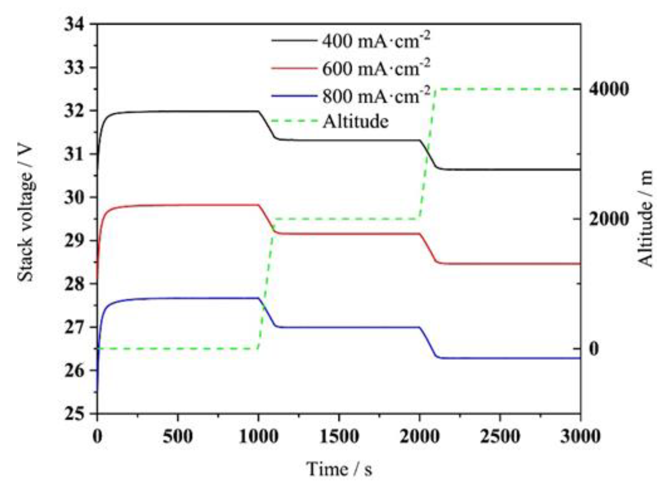
4.4. Effect of Altitude

According to [35], the effect of ambient density can be estimated by correcting the current density with the ratio of the reference pressure at sea level to the pressure at the given altitude. However, this correction is not sufficient to account for the measured increase in the maximum current density. This suggests that the concentration losses should also be corrected to account for the differences in temperature, pressure, and relative humidity.

A numerical study of the effect of altitude on PEM fuel cells at the level of a single cell is reported in [96]. For the PEMFC system, the authors considered horizontal flight at different altitudes with constant temperatures of the stack. Then, they considered a horizontal flight at 2500 m and studied the effect of humidity.

In this study, a static approach was considered for the polarization losses using the equations reported in Section 3 combined with the kinetic theory of gases and ionic conductivity analysis. Gonzalez-Espasadin et al. [96] analyzed the loss of voltage of the fuel cell, which was explained by the effect of low pressure at the cathode on the activation losses and the ideal potential. Moreover, the change in temperature affects the relative humidity. In particular, a decrease in the temperature of the cell determines a reduction in the relative humidity of the cathode, which produces better hydration of the membrane [96]. If the temperature increases and humidity decreases, the proton conductivity is reduced, causing an increase in the ohmic losses and, therefore, worsening of the cell performance. Using the numerical polarization curves of a single-cell PEM with a working temperature of 80 °C [96], it is possible to estimate a reduction in the cell power by 20% at 3000 m and 30% at 8000 m. The loss of power appears less relevant when the fuel cell works at a lower temperature (50 °C). However, these results are obtained on a single cell with a model that could be unsuitable to model the behavior of the whole fuel cell system, as pointed out by the authors of [96].

The positive effect of relative humidity on the fuel cell performances is also analyzed in [96]. The positive effect of increasing humidity is less significant when RH is greater than 60%, suggesting that the cell has reached maximum hydration.

Barelli et al. [66] implemented, in AspenPlus, a semi-empirical model of a fuel cell based on an experimentally fitted reference polarization curve obtained at standard conditions. The effects of pressure, RH, temperature, and humidity are expressed in terms of deviation from the reference polarization curve.

After validating their single-cell model with experimental data at sea level, the authors of [94] numerically analyzed the effect of increasing altitude to 2000 m and 4000 m on the performances of an OCPEMFC (see Figure 11).

To obtain such curves, the authors of [94] included the effect of temperature and pressure in the polarization curves using Equation (9) for the Nernst potential, Equation (21) for the internal resistance, Equation (16) for the activation losses and Equation (23) with K = 1 for the concentration voltage drop. The dynamics of the double-layer charging, flow rates, and stack temperature were included in the model. They obtained a reduction of about 8% in the maximum electric power with an altitude increase from sea level to 4000 m as a consequence of the reduced partial pressure of oxygen. They also underlined the dynamic response of the stack voltage to changes in altitude and found out the system stabilizes after 100 s and that the cell voltage distribution is slightly less homogeneous in case of a sudden increase in altitude. In [94], the effect of the air stoichiometric ratio is also analyzed, and it was pointed out that the minimal air stoichiometric ratio must be reduced at higher altitudes to keep the stack temperature constant. Increasing the altitude determines an increase in temperature difference between the stack and the surrounding air; see Equation (17). However deep in the analysis of the altitude effect this work is, it lacks experimental validation because the model is validated only at sea level under a single operating condition.

As shown by this analysis of the state of the art, the effect of altitude on the performance of an OCPEMFC is still not fully addressed in the scientific literature.

The dependence of stack voltage on temperature, pressure, and water content is expressed in [58] as:

$$V_{cell}=E_{Nernst}\left(p_{amb}, T_{stack}\right)-\mathsf{\Delta }{V}_{act}\left(p_{amb}, T_{stack}\right)-\mathsf{\Delta }{V}_{Ohm}\left(T_{stack}, {\lambda }_m\right)-\mathsf{\Delta }{V}_{conc}(p_{amb}, T_{stack})$$

(79)

Other dependences from ambient conditions can be added from the equations reported in Section 4. The internal resistance is affected not only by temperature and humidity but also by ambient pressure [104]. The temperature of the $T_{stack}$ in equilibrium conditions is established by controlling the fan speed, but it is influenced by ambient temperature during transients. Moreover, the effect of altitude is not only on the polarization curve of the stack but also on its balance of plan components like the fan and the fuel system [61]. The authors of [61] developed an altitude test method making use of an opened system altitude chamber. The testbench was used to obtain trends in temperature, cooling fan speed, airflow, and fuel flow at different loads and altitudes (up to 1500 m). However, only the pressure was controllable in this system. The fuel cell was not meant for propulsion but to replace the traditional aircraft battery or the conventional auxiliary power unit. The fuel cell considered in the text was a 1.2 kW Ballard Nexa unit. The authors found that as ambient temperature increases or ambient pressure decreases, the cooling fan needs to operate at a higher speed to maintain the same amount of heat transfer for a given load because of the lower density of the air. The increased speed of the fan determines larger parasitic loads and reduces the net power of the fuel cell system. The PWM duty cycle of the fan was found to increase from 54% of the maximum speed at 400 m to 72% at 1500 m to maintain the stack temperature at 65 °C. This is in accordance with the fan laws (Equation (61)).

5. Identification of the Best Simulation Approach

The effects of altitude on the whole fuel cell system are summarized in

Table 4. Summary of the effects of ambient conditions and how to model them.

Component	Parameter	Ambient Temperature	Ambient Pressure	Relative Humidity
Stack	Nernst voltage	$\mathrm{Sec}\mathrm{ondary} \mathrm{through} T_{stack}$ during transients, Equation (9)	Primary. Equation (9)	$\mathrm{Sec}\mathrm{ondary}, \mathrm{through} p_{O_2}$
	Activation losses	$\mathrm{Sec}\mathrm{ondary} \mathrm{through} T_{stack}$ during transients, Equation (16) $\mathrm{Sec}\mathrm{ondary} \mathrm{through} I_0,$ Equation (15)	Primary through Equation (19) or secondary through Equation (26)
	Ohmic losses	$\mathrm{Sec}\mathrm{ondary} \mathrm{through} T_{stack}$ during transients Equation (21)	Secondary, not modeled	$\mathrm{Indirect} \mathrm{through} {\lambda }_m$ Equation (21)
	Concentration losses	$\mathrm{Sec}\mathrm{ondary} \mathrm{through} T_{stack}$ during transients, Equation (23)	$\mathrm{Sec}\mathrm{ondary}, \mathrm{through} p_{O_2}$ Equation (24)
Cooling system	Air flow rate and PWM duty cycle	Primary from thermal balance under static, Equation (43), or dynamic conditions, Equation (66),	Primary through air density, Equation (47)	(47)
	Fan power	Primary through air density, Equation (64) or (65)	Primary through air density, Equation (64) or (65)	Secondary through air density, e Equation (64) or (65)
Purging system	Hydrogen utilization	Negligible	Primary through Equation (33) or (34)	Negligible

together with the equation that can be used to predict such effect. They are classified into primary and secondary according to their relative importance. From this point of view, the simulation approach used by Gong et al. [94] is the more complete.

By implementing these equations, it should be possible to assess the behavior of the whole fuel cell system under variable operating conditions in terms of flight altitude. However, these models include many parameters to be tuned.

The identification of the model parameters is usually performed by considering one single polarization curve, but this is not correct because the polarization curve is strongly affected by operating conditions (pressure, temperature, and humidity). Nevertheless, this approach is often found in the scientific literature. In [105], three different values of pressure and temperature are used for the parameter identification of the voltage–current curve, but the identification is repeated for each condition, so the model has no predictive value. Their model is based on empirical correlations that do not consider the operating pressure. In [36], frequency identification is applied by using data from electrochemical impedance spectroscopy.

These procedures can be affected by uncertainties in the specification of the fuel cell systems and/or in the operating conditions.

5.1. Uncertainties in the Specification of Fuel Cell Stacks

To apply the models summarized in Table 4, some geometrical parameters are needed. However, the values reported in the scientific literature are sometimes inconsistent. To underline the uncertainties in the specification of the same stack, let us consider some commercial fuel cells. In the first studies of dynamic models for fuel cells [43], the most studied PEM fuel cells were the Ballard-Mark-V and VI [26,44,48], while in more recent years, the focus has moved on the Horizon technology [57,64,65,80,88].

The number of cells in the stack is easy to retrieve because it is reported in the manual. Nevertheless, the number of cells of the H-2000 stack is reported to be 72 in Barreras et al., 2012 [6] while the value declared in the manual (and used in all other studies on this stack) is 48.

One of the pieces of information that is always necessary for applying semi-empirical models is the active area that allows passing from the current stack in A to the specific current in A/cm² as necessary to apply the voltage model. However, the active area of the Horizon H-2000 stacks is assumed to be equal to 100 cm² in Mahjoubi et al., 2019 [80] and 333 cm² in Ou et al., 2017 [88], while for the Nexa FC [44], the active area ranges from 100 cm² [94] to 122 cm². For this reason, it is considered a parameter to be estimated in [44].

More consistent is the value of membrane thickness that, for the stacks of the Horizon H series, ranges from 0.025 cm for the H-1000 [64] to 0.0238 cm for the H-2000 [88]. According to [44], most manufacturers of PEMFC use membranes of Nafion type that have a thickness between 51 and 254 μm.

The specific heat of the Horizon H-2000 stack is reported to be equal to 300 J/kgK in Mahjoubi et al., 2019 [80] and 1226 J/kgK in Ou et al., 2017 [88]. The second value seems to be more acceptable since this parameter should be independent of the stack size and values between 1240 and 1260 J/kgK are proposed for the H-500 and the H-1000 in other investigations (Kandidayeni et al. [36], Omran et al. [57], Zhang et al., 2020 [90]).

Uncertainties can also be found in other thermal parameters like the natural convection parameters and the heat exchange surface for natural and forced convection.

5.2. Uncertainties in the Operating Conditions

The semi-empirical models presented in this review require the definition of a certain number of parameters using in situ characterization techniques where signals of voltage, current, temperature, etc., are collected and used for the tuning. Most voltage models are validated/fitted only over a non-specified operating point in terms of temperature and humidity (see, for example, [57]). However, this is not correct as pointed out in [36] because of the strong effect of temperature and humidity over the polarization curve. A more correct approach is adopted in [67], where the authors considered four sets of voltage curves; two of them are used for the parameter identification process while the other two are employed to check the validity of the obtained model. Their model was found to predict accurately the effect of pressure on the voltage curve. The authors of [70] validated their model by considering three different values of the stack temperature. In their study, the only empirical variable was the gain factor used to correct the term $B$ in the modeling of the concentration losses (see Equation (23)).

In [1], the testing conditions reported in the document include warm-up (to ensure that the cell system has reached equilibrium temperature), temperature, pressure, flow rates, and compression force. Regarding the last item, compression forces must be monitored because cells with lower compression forces are characterized by increased ohmic losses while a too-high compression force can increase the concentration losses. In this analysis, the combination of the Kalman filter with Amphlett’s model was found to achieve the most precise prediction of the polarization curve.

Even fewer details are reported in the case of dynamic tests [9]. The work of Headly et al. [106] is the only investigation that proposes a validation of a model of relative humidity by comparison with transient measurements of the relative humidity at the cathode outlet.

In [64], a Horizon H-1000 PEM fuel cell stack was tested under standard pressure and 23 °C ambient temperature operated for about 25 min. The load current was increased from 1 to 17A with a holding time of one and a half minutes. A temperature sensor was installed at the exit of the fan outlet. In this work, an overall efficiency of 84% was assumed to match the experimental voltage–current curve at 23 °C, which is quite different from the manufacturer’s voltage–current curve (obtained at the nominal temperature of 25 °C).

Figure 12 shows the voltage–current curve of the H-2000 Horizon fuel cell as reported by different works in the literature compared with the nominal curve found in the manual of the manufacturer. The voltage–current curves reported in the documents significantly differ from those reported in the fuel cell datasheet because of different operating conditions in terms of pressure, temperature, and humidity of the stack. Figure 12 was drawn to put into evidence how the literature on this topic often lacks scientific rigor in neglecting to report the operating conditions of the test and in using a single polarization curve to tune or validate a model. Note that in the case of Barreras et al. [6], the polarization curve reported in their paper is not coherent with the specification of the H-2000 stack and with the number of cells in the stack.

5.3. Uncertainties in the Values of the Empirical Parameter

The estimation of the model parameters must be performed properly to avoid numerical and approximation errors. Hoogendoorn et al. [60] performed a sensitivity analysis on the empirical parameters of Equation (25) and showed that the results in terms of polarization curve are strongly affected by the value assigned to each parameter. More specifically, the parameters that had the highest impact on the voltage/current curve were the internal resistance and the Nernst voltage. Parameter $A$, which quantifies the activation losses, was also found to have a strong effect on the polarization curve, while $m$ and $n$ influence the high-current part of the voltage curve and the concentration losses dominate. A similar approach is used by [68] regarding parameters ${\xi }_i$ of Equation (16). These two investigations demonstrate that an experimental polarization curve can be fitted with different combinations of the empirical parameters, especially if a single experimental curve obtained under unspecified operating conditions is used for the tuning. The result can be a perfectly tuned model but unrealistic values of the losses and no prediction capability. Under these circumstances, the obtained model is quite useless and could be replaced by a simple look-up table implementing the experimental polarization curve.

The least squares MATLAB algorithm is applied for the fitting of the voltage–current model in [60] while genetic algorithms and particle swarm optimization evolutionary algorithms are mentioned in [44]. Reviews of the fitting procedures for the empirical coefficients reported above are included in [67], while in [36], three methods for online identification (recursive least squares, Kalman filter, and extended Kalman filter) are compared. A hybrid vortex search algorithm and differential evolution are adopted in [67]. The sum squared deviation between experimental and calculated static voltage–current curves of PEMFC is used as a fitness function to be minimized in this work. Seleem et al. [107] proposed a novel and simplified precise model for the PEMFCs parameter extraction of a fuel cell dynamic. The unknown model parameters were reduced to four and could be obtained using the meta-heuristic algorithm (also called the equilibrium optimizer).

In [96], the fitting was performed concerning only two parameters: the contact resistance $R_c$ and the temperature-independent transfer coefficient term in the activation losses. In [36], a review of metaheuristic-based algorithms for parameter estimation in terms of ${\xi }_i, i=\mathrm{1,4},\lambda ,R_c,B,I_{max}$ is reported for some fuel cell stacks with nominal power between 200 and 500 W. A review and detailed comparison of the different identification techniques for semi-empirical voltage models can be found in [108]. It was found that evolving metaheuristic techniques perform better than evolutionary algorithms.

Real-time processing of experimental data has been suggested to adapt the PEMFC model to changes in operating condition, degradation, and aging [36]. The data to extract include the maximum efficiency point, maximum power, minimum voltage, maximum current, etc. A global energy management strategy that compares the estimated with the measured value of the fuel cell voltage to update the model parameter and optimize the energy management is proposed in [36].

Kandidayeni et al. [109] proposed an online identification method able to adapt the parameters to the model according to the fuel cell aging processes. The proposed method uses the current, temperature, and pressure of the stack as inputs and the voltage of the stack as an output. There are eight parameters to be identified:${\xi }_i \mathrm{w}\mathrm{i}\mathrm{t}\mathrm{h} i=\mathrm{1,4}$ for Equation (16), ${\zeta }_1,{\zeta }_2,{\zeta }_3$ for the internal resistance, Equation (22), and $B$ for the concentration voltage drop, Equation (23).

The approach was extended in [110] and allowed the correction of the maximum current $I_{max}$ on the basis of variable operating conditions and degradation processes.

5.4. From Dynamic Models to Digital Twins

Given the difficulties in developing comprehensive dynamic models of fuel cell systems and the need for online identification methods, the natural transition of the dynamic models described in this investigation would be the development of digital twins (DT). Using DTs, for example, the designer can see if the temperature control system is performing as intended and make improvements based on real-time feedback from sensors. The critical issue in this application is the data collection from multi-physic fields including gas reactant, water content, temperature, etc. [111].

At this time, only a few works on digital twins of fuel cells can be found in the scientific literature [111,112,113]. In [111], a 3D physical model of a PEM FC is used to train a surrogate model with comparable accuracy and much higher computing efficiency. The digital twin was represented in the form of multi-physics field contours and had the goal of predicting health operation envelopes of relevant parameters like temperature, relative humidity, oxygen concentration, and liquid saturation, while in [112], the digital twin was used to predict the fuel cell remaining life. In [114,115], the concept of digital twins has been applied to a fuel cell hybrid electric vehicle to evaluate the impact of auxiliary systems on the driving range and to test different energy management strategies. In [116], a digital twin was used to predict voltage, temperature, and membrane water content for in situ operation control. In [117], a digital twin was used to predict fuel cell degradation and voltage and temperature were considered as the operation parameters to monitor the degradation level. The digital twin framework proposed by Yue et al. [117] for a fuel cell system includes a first phase in which knowledge from historical operation data, operating conditions, and human expertise is transferred to the digital twin. In a second phase, the sensors on the physical system send information to the digital twin about real-time operation data and ambient conditions. The digital twin, finally, sends commands to the physical system to perform optimizations, control actions, maintenance schedules, etc.

A suggested list of the potential application of digital twins of fuel cell systems for UAV, UAM, and lightweight aerial vehicles in general is as follows:

• Monitor the deviation of the behavior of the single component from design conditions due to degradation and aging;
• Analyze the effect of flight speed and altitude and degradation on the voltage curve and in particular on the maximum current [110] of the fuel cell;
• Manage transient and cold-start operations;
• Predict the fan power and purging process on the performance of the system to optimize efficiency and power utilization [9] and, therefore, the range, in real time during the flight;
• Implement algorithms for energy management in hybrid electric configurations or route optimization in fleet analyses [118].

6. Conclusions

This review analyzed semi-empirical models for open-cathode fuel cell systems adopted in low-power aerial vehicles and in particular their suitability to predict the behaviors of an OCPEMFC under dynamic operating conditions of load and flight altitude. The review included not only the prediction of the polarization curve of the stack but also the impact on the fuel cell performance of the balance of the plant, consisting of a forced convection air-cooling system and a water content control circuit.

Regarding the quasi-static behavior of OCPEMFCs, the analysis of the scientific literature on this topic showed that a consolidated approach has been reached in the modeling of the polarization losses, at least for operation at sea level. However, the proposed tuning and validation procedure shows some inconsistencies in terms of geometrical and operational parameters. Stack models fitted over a single polarization curve have a limited prediction capability, especially when applied under variable altitude conditions. These results stress the necessity of proposing a standardized fitting procedure that encompasses different operating conditions. The fan operation and the purging process affect the net power of the fuel cell system and its actual hydrogen consumption. Nevertheless, this aspect is seldom taken into account.

Many transient phenomena take place in OCPEMFCs and affect their response to dynamic loads. However, an all-inclusive dynamic model covering all these phenomena is still missing according to the analysis of the scientific literature performed in this paper. This lack of a global model can be justified by the different time constants of the dynamic processes, which allow some dynamic effects to be neglected according to the focus of the control action.

Recent studies on OCPEMFCs propose online identification strategies and advanced control methods to overcome the drawbacks of standard PID controllers. The working temperature of the fuel cell, which was kept constant in the first studies on the control of OCPEMFC, is considered in recent studies as a parameter to be adapted to operating conditions. The scientific research on the effect of altitude on the performance and the dynamic behavior of OCPEMFCs is still quite limited, and the adoption of altitude chambers to quantify this effect needs to be encouraged. Given the high uncertainties on the geometric and operating parameters of OCPEMFCs, a transition from dynamic models to digital twins is proposed as a future direction in this field of research.

References

1. Xu, L.; Huangfu, Y.; Ma, R.; Xie, R.; Song, Z.; Zhao, D.; Yang, Y.; Wang, Y.; Xu, L. A Comprehensive Review on Fuel Cell UAV Key Technologies: Propulsion System, Management Strategy, and Design Procedure. IEEE Trans. Transp. Electrif. 2022, 8, 4118–4139. [Google Scholar] [CrossRef]
2. Xiao, C.; Wang, B.; Zhao, D.; Wang, C. Comprehensive investigation on Lithium batteries for electric and hybrid-electric unmanned aerial vehicle applications. Therm. Sci. Eng. Prog. 2023, 38, 101677. [Google Scholar] [CrossRef]
3. Zakhvatkin, L.; Schechter, A.; Avrahami, I. Water Recuperation from Hydrogen Fuel Cell during Aerial Mission. Energies 2022, 15, 6848. [Google Scholar] [CrossRef]
4. O’Hayre, R.; Colella, W.; Cha, S.-W.; Prinz, F.B. Fuel Cell Fundamentals; Wiley: Hoboken, NJ, USA, 2016. [Google Scholar]
5. Larmine, J.; Dicks, A. Fuel Cell Systems Explained; Wiley: Hoboken, NJ, USA, 2003; ISBN 9780470848579. [Google Scholar]
6. Barreras, F.; Lozano, A.; Barroso, J.; Roda, V.; Maza, M. Theoretical Model for the Optimal Design of an Air cooling System of Polymer Electrolyte Fuel cell. Application for a High-temperature PEMFC. Fuel Cells 2013, 13, 227–237. [Google Scholar] [CrossRef]
7. Squadrito, G.; Maggio, G.; Passalacqua, E.; Lufrano, F.; Patti, A. An empirical equation for polymer electrolyte fuel cell (PEFC) behaviour. J. Appl. Electrochem. 1999, 29, 1449–1455. [Google Scholar] [CrossRef]
8. Ishaku, J.; Lotfi, N.; Zomorodi, H.; Landers, R.G. Control-oriented modeling for open-cathode fuel cell systems. In Proceedings of the 2014 American Control Conference—ACC 2014, Portland, OR, USA, 4–6 June 2014; pp. 268–273. [Google Scholar]
9. Nóbrega, P.H.A. A review of physics-based low-temperature proton-exchange membrane fuel cell models for system-level water and thermal management studies. J. Power Sources 2023, 558, 232585. [Google Scholar] [CrossRef]
10. Wright, S.; Aaltonen, J. Fuel cells and novel thermal management advancements required for aviation. In Proceedings of the 33rd Congress of the International Council of the Aeronautical Sciences ICAS2022, Stockholm, Sweden, 4–9 September 2022; The International Council of the Aeronautical Sciences: Bonn, Germany, 2022. [Google Scholar]
11. Nexa™ (310-0027) Power Module User’s Manual MAN5100078. Available online: http://faculty.stust.edu.tw/~wcchang/MAN5100078.pdf (accessed on 5 September 2023).
12. Kim, T.; Kwon, S. Design and development of a fuel cell-powered small unmanned aircraft. Int. J. Hydrogen Energy 2012, 37, 615–622. [Google Scholar] [CrossRef]
13. Pratt, J.W.; Brouwer, J.; Samuelsen, G.S. Performance of proton exchange membrane fuel cell at high-altitude conditions. J. Propuls. Power 2007, 23, 437–444. [Google Scholar] [CrossRef]
14. Wang, Y.-X.; Chen, Q.; Zhang, J.; He, H. Real-time power optimization for an air-coolant proton exchange membrane fuel cell based on active temperature control. Energy 2021, 220, 119497. [Google Scholar] [CrossRef]
15. Chen, F.; Yu, Y.; Gao, Y. Temperature Control for Proton Exchange Membrane Fuel Cell based on Current Constraint with Consideration of Limited Cooling Capacity. Fuel Cells 2017, 17, 662–670. [Google Scholar] [CrossRef]
16. Tolj, I.; Penga, Ž.; Vukičević, D.; Barbir, F. Thermal management of edge-cooled 1 kW portable proton exchange membrane fuel cell stack. Appl. Energy 2020, 257, 114038. [Google Scholar] [CrossRef]
17. Xing, S.; Zhao, C.; Zou, J.; Zaman, S.; Yu, Y.; Gong, H.; Wang, Y.; Chen, M.; Wang, M.; Lin, M.; et al. Recent advances in heat and water management of forced-convection open-cathode proton exchange membrane fuel cells. Renew. Sustain. Energy Rev. 2022, 165, 112558. [Google Scholar] [CrossRef]
18. Zakhvatkin, L.; Schechter, A.; Buri, E.; Avrahami, I. Edge Cooling of a Fuel Cell during Aerial Missions by Ambient Air. Micromachines 2021, 12, 1432. [Google Scholar] [CrossRef] [PubMed]
19. Rathke, P.; Thalau, O.; Kallo, J.; Schirmer, J.; Stephan, T. Long Distance Flight Testing with the Fuel Cell Powered Aircraft Antares DLR-H2. In Proceedings of the Deutscher Luft- und Raumfahrtkongress, Stuttgart, Germany, 10–12 September 2013; Deutsche Gesellschaft für Luft-und Raumfahrt-Lilienthal-Oberth eV.: Bonn, Germany, 2013. Document ID: 301219. [Google Scholar]
20. Dudek, M.; Raźniak, A.; Rosół, M.; Siwek, T.; Dudek, P. Design, Development, and Performance of a 10 kW Polymer Exchange Membrane Fuel Cell Stack as Part of a Hybrid Power Source Designed to Supply a Motor Glider. Energies 2020, 13, 4393. [Google Scholar] [CrossRef]
21. De Bernardinis, A.; Péra, M.C.; Garnier, J.; Hissel, D.; Coquery, G.; Kauffmann, J.M. Fuel cells multi-stack power architectures and experimental validation of 1 kW parallel twin stack PEFC generator based on high frequency magnetic coupling dedicated to on board power unit. Energy Convers. Manag. 2008, 49, 2367–2383. [Google Scholar] [CrossRef]
22. Romeo, G.; Cestino, E.; Correa, G.; Borello, F. A fuel cell-based propulsion system for general aviation aircraft: The ENFI-CA-FC experience. SAE Int. J. Aerosp. 2011, 4, 724–737. [Google Scholar] [CrossRef]
23. Geliev, A.; Varyukhin, A.; Zakharchenko, V.; Kiselev, I.; Zhuravlev, D. Conceptual Design of an Electric Propulsion System Based on Fuel Cells for an Ultralight Manned Aircraft. In Proceedings of the 2019 International Conference on Electrotechnical Complexes and Systems (ICOECS), Ufa, Russia, 21–25 October 2019; pp. 1–17. [Google Scholar]
24. Donateo, T. Semi-Empirical Models for Stack and Balance of Plant in Closed-Cathode Fuel Cell Systems for Aviation. Energies 2023, 16, 7676. [Google Scholar] [CrossRef]
25. Zhu, K.-Q.; Ding, Q.; Xu, J.-H.; Yang, C.; Zhang, J.; Zhang, Y.; Huang, T.-M.; Wan, Z.-M.; Wang, X.-D. Dynamic performance for a kW-grade air-cooled proton exchange membrane fuel cell stack. Int. J. Hydrogen Energy 2022, 47, 35398–35411. [Google Scholar] [CrossRef]
26. Saadi, A.; Becherif, M.; Hissel, D.; Ramadan, H. Dynamic modeling and experimental analysis of PEMFCs: A comparative study. Int. J. Hydrogen Energy 2017, 42, 1544–1557. [Google Scholar] [CrossRef]
27. Zeng, T.; Zhang, C.; Huang, Z.; Li, M.; Chan, S.H.; Li, Q.; Wu, X. Experimental investigation on the mechanism of variable fan speed control in Open cathode PEM fuel cell. Int. J. Hydrogen Energy 2019, 44, 24017–24027. [Google Scholar] [CrossRef]
28. Wu, D.; Peng, C.; Yin, C.; Tang, H. Review of System Integration and Control of Proton Exchange Membrane Fuel Cells. Electrochem. Energy Rev. 2020, 3, 466–505. [Google Scholar] [CrossRef]
29. Yang, C.-W.; Chen, Y.-S. A mathematical model to study the performance of a proton exchange membrane fuel cell in a dead-ended anode mode. Appl. Energy 2014, 130, 113–121. [Google Scholar] [CrossRef]
30. Strahl, S.; Husar, A.; Puleston, P.; Riera, J. Performance Improvement by Temperature Control of an Open-Cathode PEM Fuel Cell System. Fuel Cells 2014, 14, 466–478. [Google Scholar] [CrossRef]
31. Bradley, T.H.; Moffitt, B.A.; Mavris, D.N.; Parekh, D.E. Development and experimental characterization of a fuel cell powered aircraft. J. Power Sources 2007, 171, 793–801. [Google Scholar] [CrossRef]
32. Lin, Y.-F.; Chen, Y.-S. Experimental study on the optimal purge duration of a proton exchange membrane fuel cell with a dead-ended anode. J. Power Sources 2017, 340, 176–182. [Google Scholar] [CrossRef]
33. Zhao, D.; Xia, L.; Dang, H.; Wu, Z.; Li, H. Design and control of air supply system for PEMFC UAV based on dynamic decoupling strategy. Energy Convers. Manag. 2022, 253, 115159. [Google Scholar] [CrossRef]
34. Peng, H.; Stefanopoulou, A.G. Simulation and analysis of transient fuel cell system performance-based on a dynamic reactant flow model. In Proceedings of the IMECE’02, ASME International Mechanical Engineering Congress & Exposition, New Orleans, LA, USA, 17–22 November 2002. [Google Scholar]
35. Atkinson, R.W.; Hazard, M.W.; Rodgers, J.A.; Stroman, R.O.; Gould, B.D. An Open-Cathode Fuel Cell for Atmospheric Flight. J. Electrochem. Soc. 2017, 164, F46–F54. [Google Scholar] [CrossRef]
36. Kandidayeni, M.; Macias, A.; Amamou, A.; Boulon, L.; Kelouwani, S.; Chaoui, H. Overview and benchmark analysis of fuel cell parameters estimation for energy management purposes. J. Power Sources 2018, 380, 92–104. [Google Scholar] [CrossRef]
37. Sun, L.; Jin, Y.; You, F. Active disturbance rejection temperature control of open-cathode proton exchange membrane fuel cell. Appl. Energy 2020, 261, 114381. [Google Scholar] [CrossRef]
38. Hu, M.; Zhao, R.; Pan, R.; Cao, G. Disclosure of the internal mechanism during activating a proton exchange membrane fuel cell based on the three-step activation method. Int. J. Hydrogen Energy 2021, 46, 3008–3021. [Google Scholar] [CrossRef]
39. Zhan, Y.; Guo, Y.; Zhu, J.; Liang, B.; Yang, B. Comprehensive influences measurement and analysis of power converter low frequency current ripple on PEM fuel cell. Int. J. Hydrogen Energy 2019, 44, 31352–31359. [Google Scholar] [CrossRef]
40. Tan, B.; Chen, H.; Quan, R.; Quan, S.; Zhou, Y. Study on data-driven PEMFC humidity mechanism soft-sensing model. J. Phys. Conf. Ser. 2019, 1423, 012043. [Google Scholar] [CrossRef]
41. Guzzella, L.; Sciarretta, A. Vehicle Propulsion Systems, Introduction to Modeling and Optimization, 3rd ed.; Springer: Berlin/Heidelberg, Germany, 2013. [Google Scholar]
42. Ren, P.; Pei, P.; Li, Y.; Wu, Z.; Chen, D.; Huang, S. Degradation mechanisms of proton exchange membrane fuel cell under typical automotive operating conditions. J. Prog. Energy Combust. Sci. 2020, 80, 100859. [Google Scholar] [CrossRef]
43. Wang, C.; Nehrir, M.; Shaw, S. Dynamic Models and Model Validation for PEM Fuel Cells Using Electrical Circuits. IEEE Trans. Energy Convers. 2005, 20, 442–451. [Google Scholar] [CrossRef]
44. Restrepo, C.; Konjedic, T.; Garces, A.; Calvente, J.; Giral, R. Identification of a Proton-Exchange Membrane Fuel Cell’s Model Parameters by Means of an Evolution Strategy. IEEE Trans. Ind. Inform. 2015, 11, 548–559. [Google Scholar] [CrossRef]
45. Boukoberine, M.N.; Zia, M.F.; Benbouzid, M.; Zhou, Z.; Donateo, T. Hybrid fuel cell powered drones energy management strategy improvement and hydrogen saving using real flight test data. Energy Convers. Manag. 2021, 236, 113987. [Google Scholar] [CrossRef]
46. Boukoberine, M.N.; Donateo, T.; Benbouzid, M. Optimized energy management strategy for hybrid fuel cell powered drones in persistent missions using real flight test data. IEEE Trans. Energy Convers. 2022, 37, 2080–2091. [Google Scholar] [CrossRef]
47. Ou, K.; Wang, Y.; Kim, Y. Performance Optimization for Open-cathode Fuel Cell Systems with Overheating Protection and Air Starvation Prevention. Fuel Cells 2017, 17, 299–307. [Google Scholar] [CrossRef]
48. Lee, C.-H.; Yang, J.-T. Modeling the Ballard-Mark-5 proton exchange membrane fuel cell with power converters for applications in autonomous underwater vehicles. J. Power Sources 2011, 196, 3810–3823. [Google Scholar] [CrossRef]
49. Vandana, G.A.; Panigrahi, B.K. Multi-dimensional digital twin of energy storage system for electrical vehicles: A brief review. Energy Storage Early View 2021, 3, e242. [Google Scholar] [CrossRef]
50. Bhatti, G.; Mohan, H.; Singh, R. R Towards the future of smart electric vehicles: Digital twin technology. Renew. Sustain. Energy Rev. 2021, 141, 110801. [Google Scholar] [CrossRef]
51. Li, Y.; Wang, S.; Duan, X.; Liu, S.; Liu, J.; Hu, S. Multi-objective energy management for Atkinson cycle engine and series hybrid electric vehicle based on evolutionary NSGA-II algorithm using digital twins. Energy Convers. Manag. 2021, 230, 113788. [Google Scholar] [CrossRef]
52. Kamran, S.S.; Haleem, A.; Bahl, S.; Javaid, M.; Nandan, D.; Verma, A.S. Role of smart materials and digital twin (DT) for the adoption of electric vehicles in India. Mater. Today Proc. 2022, 52, 2295–2304. [Google Scholar] [CrossRef]
53. Glaessgen, E.; Stargel, D. The digital twin paradigm for future NASA and U.S. Air DT9 Force vehicles. In Proceedings of the 53rd AIAA/ASME/ASCE/AHS/ASC structures, Structural Dynamics and Materials Conference, Honolulu, HI, USA, 23–26 April 2012. [Google Scholar]
54. Subin, K.; Jithesh, P.K. Experimental study on self-humidified operation in PEM fuel cells. Sustain. Energy Technol. Assess. 2018, 27, 17–22. [Google Scholar] [CrossRef]
55. Abul-Hawa, A.A.; Ebaid, M.S.; Bhinder, F.S.; Calay, R.K. Control strategy for polymer electrolyte membrane fuel cell system. In Proceedings of the 2006 UKACC International Conference on Control, Glasgow, UK, 30 August–1 September 2006; p. 94. [Google Scholar]
56. Le, P.-L.; Singh, B.; Chen, Y.-S.; Arpornwichanop, A. An experimental study for optimizing the energy efficiency of a proton exchange membrane fuel cell with an open-cathode. Int. J. Hydrogen Energy 2021, 46, 26507–26517. [Google Scholar] [CrossRef]
57. Omran, A.; Lucchesi, A.; Smith, D.; Alaswad, A.; Amiri, A.; Wilberforce, T.; Sodré, J.R.; Olabi, A. Mathematical model of a proton-exchange membrane (PEM) fuel cell. Int. J. Thermofluids 2021, 11, 100110. [Google Scholar] [CrossRef]
58. Choe, S.-Y.; Ahn, J.-W.; Lee, J.-G.; Baek, S.-H. Dynamic Simulator for a PEM Fuel Cell System with a PWM DC/DC Converter. IEEE Trans. Energy Convers. 2008, 23, 669–680. [Google Scholar] [CrossRef]
59. Djerioui, A.; Houari, A.; Zeghlache, S.; Saim, A.; Benkhoris, M.F.; Meshabi, T.; Machmoum, M. Energy management strategy of Supercapacitor/Fuel Cell energy storage devices for vehicle applications. Int. J. Hydrogen Energy 2019, 44, 23416–23428. [Google Scholar] [CrossRef]
60. Hoogendoorn, J. Fuel Cells and Battery Hybrid System Optimization. Master’s Thesis in Aerospace Engineering, DELFT University of Technology, Delft, The Netherlands, 2018. [Google Scholar]
61. Chang, V.; Gallman, J. Altitude Testing of Fuel Cell Systems for Aircraft Applications. Power Systems Conference. J. Aerosp. 2004, 113, 1943–1957. [Google Scholar]
62. Verstraete, D.; Lehmkuehler, K.; Gong, A.; Harvey, J.R.; Brian, G.; Palmer, J.L. Characterisation of a hybrid, fuel-cell-based propulsion system for small unmanned aircraft. J. Power Sources 2014, 250, 204–211. [Google Scholar] [CrossRef]
63. Donateo, T.; Pacella, D.; Indiveri, G.; Ingrosso, F.; Damiani, A. Dynamic Modeling of a PEM Fuel Cell for a Low Consumption Prototype. SAE Tech. Pap. 2013, 2, 1–10. [Google Scholar] [CrossRef]
64. Saleh, I.M.M.; Ali, R.; Zhang, H. Simplified mathematical model of proton exchange membrane fuel cell based on horizon fuel cell stack. J. Mod. Power Syst. Clean Energy 2016, 4, 668–679. [Google Scholar] [CrossRef]
65. Sahel, I.M.M. Modeling, Simulation and Performance Evaluation: PEM Fuel Cells for High Altitude UAS. Ph.D. Thesis, Sheffield Hallam University, Sheffield, UK, 2015. [Google Scholar]
66. Barelli, L.; Bidini, G.; Gallorini, F.; Ottaviano, A. Analysis of the operating conditions influence on PEM fuel cell performances by means of a novel semi-empirical model. Int. J. Hydrogen Energy 2011, 36, 10434–10442. [Google Scholar] [CrossRef]
67. Fathy, A.; Abd Elaziz, M.; Alharbi, A.F. A novel approach based on hybrid vortex search algorithm and differential evolution for identifying the optimal parameters of PEM fuel cell. Renew. Energy 2020, 146, 1833–1845. [Google Scholar] [CrossRef]
68. Qingshan, X.; Nianchun, W.; Ichiyanagi, K.; Yukita, K. PEM Fuel Cell modeling and parameter influences of performance evaluation. In Proceedings of the 2008 Third International Conference on Electric Utility Deregulation and Restructuring and Power Technologies, Nanjing, China, 6–9 April 2008; pp. 2827–2832. [Google Scholar]
69. Mohamed, W.W.; Kamil, M.H.M. Hydrogen preheating through waste heat recovery of an open-cathode PEM fuel cell leading to power output improvement. Energy Convers. Manag. 2016, 124, 543–555. [Google Scholar] [CrossRef]
70. Musio, F.; Tacchi, F.; Omati, L.; Stampino, P.G.; Dotelli, G.; Limonta, S.; Brivio, D.; Grassini, P. PEMFC system simulation in MATLAB-Simulink® environment. Int. J. Hydrogen Energy 2011, 36, 8045–8052. [Google Scholar] [CrossRef]
71. Barreras, F.; Lopez, A.M.; Lozano, A.; Barranco, J.E. Experimental study of the pressure drop in the cathode side of air-forced open-cathode proton exchange membrane fuel cells. Int. J. Hydrogen Energy 2011, 36, 7612–7620. [Google Scholar] [CrossRef]
72. Sasmito, A.P.; Birgersson, E.; Lum, K.W.; Mujumdar, A.S. Fan selection and stack design for open-cathode polymer electrolyte fuel cell stacks. Renew. Energy 2012, 37, 325–332. [Google Scholar] [CrossRef]
73. Arredondo, A.; Roy, P.; Wofford, E. Implementing PWM fan speed control within a computer chassis power supply. In Proceedings of the Twentieth Annual IEEE Applied Power Electronics Conference and Exposition, APEC 2005, Austin, TX, USA, 6–10 March 2005. [Google Scholar]
74. Wang, Y.-X.; Qin, F.-F.; Ou, K.; Kim, Y.-B. Temperature Control for a Polymer Electrolyte Membrane Fuel Cell by Using Fuzzy Rule. IEEE Trans. Energy Convers. 2016, 31, 667–675. [Google Scholar] [CrossRef]
75. Barroso, J.; Renau, J.; Lozano, A.; Miralles, J.; Martín, J.; Sánchez, F.; Barreras, F. Experimental determination of the heat transfer coefficient for the optimal design of the cooling system of a PEM fuel cell placed inside the fuselage of an UAV. Appl. Therm. Eng. 2015, 89, 1–10. [Google Scholar] [CrossRef]
76. Wang, Y.; Wang, C.-Y. Dynamics of polymer electrolyte fuel cells undergoing load changes. Electrochim. Acta 2006, 51, 3924–3933. [Google Scholar] [CrossRef]
77. Tahri, A.; El Fadil, H.; Belhaj, F.; Gaouzi, K.; Rachid, A.; Giri, F.; Chaoui, F. Management of fuel cell power and supercapacitor state-of-charge for electric vehicles. Electr. Power Syst. Res. 2019, 160, 89–98. [Google Scholar] [CrossRef]
78. Ríos, G.M.; Becker, F.; Vorndran, A.; Gentner, C.; Ansar, S.A. Investigation of gas purging and cold storage impact on PEM fuel cell system performance for aeronautical applications. E3S Web Conf. 2022, 334, 06004. [Google Scholar] [CrossRef]
79. Daud, W.; Rosli, R.; Majlan, E.; Hamid, S.; Mohamed, R.; Husaini, T. PEM fuel cell system control: A review. Renew. Energy 2017, 113, 620–638. [Google Scholar] [CrossRef]
80. Mahjoubi, C.; Olivier, J.-C.; Skander-Mustapha, S.; Machmoum, M.; Slama-Belkhodja, I. An improved thermal control of open cathode proton exchange membrane fuel cell. 9th International Renewable Energy Congress (IREC). Int. J. Hydrogen Energy 2019, 44, 11332–11345. [Google Scholar] [CrossRef]
81. Mirfarsi, S.H.; Parnian, M.J.; Rowshanzamir, S. Self-humidifying proton exchange membranes for fuel cell applications: Advances and challenges. Processes 2020, 8, 1069. [Google Scholar] [CrossRef]
82. Kumar, S.S.; Cirrincione, M.; Lechappe, V.; Ram, K.R.; Mohammadi, A. A Simplified Control Oriented Model of an Open Cathode PEM Fuel Cell. In Proceedings of the 2021 IEEE 12th Energy Conversion Congress & Exposition—Asia (ECCE-Asia), Singapore, 24–27 May 2021; pp. 2415–2420. [Google Scholar]
83. Wang, Y.; Wang, C.Y. Transient analysis of polymer electrolyte fuel cells. Electrochim. Acta 2005, 50, 1307–1315. [Google Scholar] [CrossRef]
84. López-Sabirón, A.M.; Barroso, J.; Roda, V.; Barranco, J.; Lozano, A.; Barreras, F. Design and development of the cooling system of a 2 kW nominal power open-cathode polymer electrolyte fuel cell stack. Int. J. Hydrogen Energy 2012, 37, 7289–7298. [Google Scholar] [CrossRef]
85. Strahl, S.; Costa-Castello, R. Temperature control of open-cathode PEM fuel cells. IFAC PapersOnLine 2017, 50, 11088–11093. [Google Scholar] [CrossRef]
86. Zhu, J.; Zou, J.; Li, X.; Peng, C. An adaptive sliding mode observer based near-optimum OER tracking control approach for PEMFC under dynamic operation condition. Int. J. Hydrogen Energy 2022, 47, 1157–1171. [Google Scholar] [CrossRef]
87. Qi, Y.; Espinoza-Andaluz, M.; Thern, M.; Li, T.; Andersson, M. Dynamic modeling and controlling strategy of polymer electrolyte fuel cells. Int. J. Hydrogen Energy 2020, 45, 29718–29729. [Google Scholar] [CrossRef]
88. Ou, K.; Yuan, W.-W.; Choi, M.; Yang, S.; Kim, Y.-B. Performance increase for an open-cathode PEM fuel cell with humidity and temperature control. Int. J. Hydrogen Energy 2017, 42, 29852–29862. [Google Scholar] [CrossRef]
89. Zhu, J.; Zhang, P.; Li, X.; Jiang, B. Robust oxygen excess ratio control of PEMFC systems using adaptive dynamic programming. Energy Rep. 2022, 8, 2036–2044. [Google Scholar] [CrossRef]
90. Zhang, B.; Lin, F.; Zhang, C.; Liao, R.; Wang, Y.-X. Design and implementation of model predictive control for an open-cathode fuel cell thermal management system. Renew. Energy 2020, 154, 1014–1024. [Google Scholar] [CrossRef]
91. Li, X.; Qi, Y.; Li, S.; Tunestal, P.; Andersson, M. A multi-input and single-output voltage control for a polymer electrolyte fuel cell system using model predictive control method. Int. J. Energy Res. 2021, 45, 12854–12863. [Google Scholar] [CrossRef]
92. Kandidayeni, M.; Macias, F.A.; Boulon, L.; Kelouwani, S. Efficiency Enhancement of an Open Cathode Fuel Cell Through a Systemic Management. IEEE Trans. Veh. Technol. 2019, 68, 11462–11472. [Google Scholar] [CrossRef]
93. Çınar, H.; Kandemir, I.; Donateo, T. Current Technologies and Future Trends of Hydrogen Propulsion Systems in Hybrid Small Unmanned Aerial Vehicles. In Hydrogen Electrical Vehicles; Scrivener Publishing LLC: Beverly, MA, USA, 2023; pp. 75–109. [Google Scholar]
94. Gong, C.; Xing, L.; Liang, C.; Tu, Z. Modeling and dynamic characteristic simulation of air-cooled proton exchange membrane fuel cell stack for unmanned aerial vehicle. Renew. Energy 2022, 188, 1094–1104. [Google Scholar] [CrossRef]
95. Song, W.J.; Chen, H.; Guo, H.; Ye, F.; Li, J.R. Research progress of proton exchange membrane fuel cells utilizing in high altitude environments. Int. J. Hydrogen Energy 2022, 47, 24945–24962. [Google Scholar] [CrossRef]
96. González-Espasandín, O.; Leo, T.J.; Raso, M.A.; Navarro, E. Direct methanol fuel cell (DMFC) and H2 proton exchange membrane fuel (PEMFC/H2) cell performance under atmospheric flight conditions of Unmanned Aerial Vehicles. Renew. Energy 2019, 130, 762–773. [Google Scholar] [CrossRef]
97. Amphlett, J.C.; Baumert, R.M.; Harris, T.J.; Mann, R.F.; Peppley, B.A.; Roberge, P.R. Performance modeling of the Ballard Mark IV solid polymer electrolyte fuel cell: I. Mechanistic model development. J. Electrochem. Soc. 1995, 142, 1. [Google Scholar] [CrossRef]
98. Corêa, J.M.; Farret, F.A.; Canha, L.N.; Simões, M.G. An Electrochemical-Based Fuel Cell Model Suitable for Electrical Engineering Automation Approach. IEEE Trans. Ind. Electron. 2004, 51, 1103–1111. [Google Scholar] [CrossRef]
99. Mann, R.F.; Amphlett, J.C.; Hooper, M.A.I.; Jensen, H.M.; Peppley, B.A.; Roberge, P.R. Development and application of a generalised steady-state electrochemical model for a PEM fuel cell. J. Power Sources 2000, 86, 173–180. [Google Scholar] [CrossRef]
100. El-Fergany, A.A. Electrical characterisation of proton exchange membrane fuel cells stack using grasshopper optimizer. IET Renew. Power Gener. 2017, 12, 9–17. [Google Scholar] [CrossRef]
101. Lee, J.; Lalk, T.; Appleby, A. Modeling electrochemical performance in large scale proton exchange membrane fuel cell stacks. J. Power Sources 1998, 70, 258–268. [Google Scholar] [CrossRef]
102. Dick, E. Dynamic Similitude. In Fundamentals of Turbomachines; Springer International Publishing: Cham, Switzerland, 2022; pp. 257–292. [Google Scholar]
103. Li, Q.; Chen, W.; Wang, Y.; Liu, S.; Jia, J. Parameter identification for PEM fuel-cell mechanism model based on effective informed adaptive particle swarm optimization. IEEE Trans. Ind. Electron. 2010, 58, 2410–2419. [Google Scholar] [CrossRef]
104. Lin, C.; Yan, X.; Wei, G.; Ke, C.; Shen, S.; Zhang, J. Optimization of configurations and cathode operating parameters on liquid-cooled proton exchange membrane fuel cell stacks by orthogonal method. Appl. Energy 2019, 253, 113496. [Google Scholar] [CrossRef]
105. Al-Othman, A.K.; Ahmed, N.A.; Al-Fares, F.S.; AlSharidah, M.E. Parameter Identification of PEM Fuel Cell Using Quantum-Based Optimization Method. Arab. J. Sci. Eng. 2015, 40, 2619–2628. [Google Scholar] [CrossRef]
106. Headley, H.; Yu, V.; Borduin, R.; Chen, D.; Li, W. Development and experimental validation of a physical-based PEM fuel cell model for cathode humidity control design. IEEE/ASME Trans. Mechatron. 2016, 21, 1775–1782. [Google Scholar] [CrossRef]
107. Seleem, S.I.; Hasanien, H.M.; El-Fergany, A.A. Equilibrium optimizer for parameter extraction of a fuel cell dynamic model. Renew. Energy 2021, 169, 117–128. [Google Scholar] [CrossRef]
108. Mitra, U.; Arya, A.; Gupta, S. A comprehensive and comparative review on parameter estimation methods for modelling proton exchange membrane fuel cell. Fuel 2023, 335, 127080. [Google Scholar] [CrossRef]
109. Kandidayeni, M.; Macias, A.; Amamou, A.A.; Boulon, L.; Kelouwani, S. Comparative analysis of two online identification algorithms in a fuel cell system. Fuel Cells 2018, 18, 347–358. [Google Scholar] [CrossRef]
110. Kandidayeni, M.; Chaoui, H.; Boulon, L.; Trovão, J.P.F. Adaptive parameter identification of a fuel cell system for health-conscious energy management applications. IEEE Trans. Intell. Transp. Syst. 2021, 23, 7963–7973. [Google Scholar] [CrossRef]
111. Wang, B.; Zhang, G.; Wang, H.; Xuan, J.; Jiao, K. Multi-physics-resolved digital twin of proton exchange membrane fuel cells with a data-driven surrogate model. Energy AI 2020, 1, 100004. [Google Scholar] [CrossRef]
112. Meraghni, S.; Terrissa, L.S.; Yue, M.; Ma, J.; Jemei, S.; Zerhouni, N. A data-driven digital-twin prognostics method for proton exchange membrane fuel cell remaining useful life prediction. Int. J. Hydrogen Energy 2021, 46, 2555–2564. [Google Scholar] [CrossRef]
113. Rassõlkin, A.; Vaimann, T.; Kallaste, A.; Kuts, V. Digital twin for propulsion drive of autonomous electric vehicle. In Proceedings of the 2019 IEEE 60th International Scientific Conference on Power and Electrical Engineering of Riga Technical University (RTUCON), Riga, Latvia, 7–9 October 2019; pp. 1–4. [Google Scholar] [CrossRef]
114. Bartolucci, L.; Cennamo, E.; Cordiner, S.; Mulone, V.; Pasqualini, F.; Aimo Boot, F. Digital Twin of Fuel Cell Hybrid Electric Vehicle: A detailed modelling approach of the hydrogen powertrain and the auxiliary systems. E3S Web Conf. 2022, 334, 06003. [Google Scholar] [CrossRef]
115. Bartolucci, L.; Cennamo, E.; Cordiner, S.; Mulone, V.; Pasqualini, F.; Boot, M.A. Digital twin of a hydrogen fuel cell hybrid electric vehicle: Effect of the control strategy on energy efficiency. Int. J. Hydrogen Energy 2023, 48, 20971–20985. [Google Scholar] [CrossRef]
116. Bai, F.; Quan, H.B.; Yin, R.J.; Zhang, Z.; Jin, S.Q.; He, P.; Mu, Y.-T.; Gong, X.-M.; Tao, W.Q. Three-dimensional multi-field digital twin technology for proton exchange membrane fuel cells. Appl. Energy 2022, 324, 119763. [Google Scholar] [CrossRef]
117. Yue, M.; Benaggoune, K.; Meng, J.; Diallo, D. Implementation of an early-stage fuel cell degradation prediction digital twin based on transfer learning. IEEE Trans. Transp. Electrif. 2022, 9, 3308–3318. [Google Scholar] [CrossRef]
118. Kandidayeni, M.; Macias, A.; Boulon, L.; Trovão, J.P.F. Online modeling of a fuel cell system for an energy management strategy design. Energies 2020, 13, 3713. [Google Scholar] [CrossRef]
Figure 1. Structure of a PEM fuel cell.
Energies 17 00900 g001
Figure 2. Recorded load power profile of a battery quadcopter [45].
Energies 17 00900 g002
Figure 3. BOP of a self-humidified OCPEMFC. No external humidification is required because of the self-humidification process.
Energies 17 00900 g003
Figure 4. Fuel utilization vs. load [62].
Energies 17 00900 g004
Figure 5. Typical curves of cell voltage, net efficiency, and net power vs. current.
Energies 17 00900 g005
Figure 6. Typical performance of a fan and an example of stack resistance curve.
Energies 17 00900 g006
Figure 7. Typical voltage curve of a fuel cell.
Energies 17 00900 g007
Figure 8. Equivalent electric circuit applied in the quasi-static analysis of PEMFCs.
Energies 17 00900 g008
Figure 9. Equivalent electric circuit with double-layer capacitor effect.
Energies 17 00900 g009
Figure 10. Equivalent circuit used for temperature dynamics by Restrepo et al. [44].
Energies 17 00900 g010
Figure 11. Simulated voltage curves of a OCPEMFC at different altitudes and currents [94].
Energies 17 00900 g011
Figure 12. Voltage–current curves of the same fuel cell stack (H-2000) as reported in different investigations [6,59,80,88].
Energies 17 00900 g012