Abstract
For hydrogen-powered vehicles, the efficiency cost brought about by the current industry choices of hydrogen storage methods greatly reduces the system’s overall efficiency. The physisorption of hydrogen fuel onto metal–organic frameworks (MOFs) is a promising alternative storage method due to their large surface areas and exceptional tunability. However, the massive selection of MOFs poses a challenge for the efficient screening of top-performing MOF structures that are capable of meeting target hydrogen uptakes. This study examined the performance of 13 machine learning (ML) models in the prediction of the gravimetric and volumetric hydrogen uptakes of real MOF structures for comparison with simulated and experimental results. Among the 13 models studied, 12 models gave an R2 greater than 0.95 in the prediction of both the gravimetric and the volumetric uptakes in MOFs. In addition, this study introduces a 4-20-1 ANN model that predicts the bulk, shear, and Young’s moduli for the MOFs. The machine learning models with high R2 can be used in choosing MOFs for hydrogen storage.
1. Introduction
Hydrogen (H2) is of particular interest in research due to the rising interest in clean energy as a response to the progression of climate change. As vehicle fuel consumption constitutes a significant percentage of fossil fuel use and, in turn, global carbon emissions, considerable interest has been invested in developing hydrogen as an energy carrier for powering light-duty, fuel cell-powered vehicles with energy derived from cleaner sources [1,2]. However, while fuel cell technology has been around for some time, the major obstacle hampering its widespread use remains the lack of efficient and economically sound storage and transportation methods for hydrogen [3,4]. The widely adopted physically based storage methods require high pressures or cryogenic temperatures, making them expensive and difficult to maintain [5,6]. The US Department of Energy (DOE) sets technical targets for on-board hydrogen storage parameters to accelerate the development of a robust hydrogen storage method. The latest target set for 2025 is a usable energy density of 1.3 kWh L−1, corresponding to 0.040 kg H2 L−1 [7]. As such, highly porous materials that readily facilitate physisorption, such as carbon materials, nanocomposites, and MOFs, are potential alternatives for storage that allow energy-efficient storage that is capable of achieving densities comparable to those of the liquid state. Furthermore, MOFs offer highly favorable kinetics that enable rapid adsorption and desorption, allowing the easy storage and use of H2 [8,9].
Metal–organic frameworks (MOFs) are porous materials that are known for their exceptional tunability. They are composed of organo-metallic hybrid bonds with metal joints serving as the primary building units (PBUs) and organic ligands or linkers serving as secondary building units (SBUs). The precise selection of the constituents allows flexibility in the modification of the physical and chemical features, in addition to general properties such as large surface areas and high porosity [10]. As such, the development of MOFs and the enhancement of their properties has been a primary research focus for further applications in gas adsorption and separation [11,12,13], storage [14,15,16], and catalysis [17,18,19,20]. However, the infinite combinations resulting from MOF tuning make the efficient screening and performance evaluation for MOFs with appropriate properties that would fit each application challenging in terms of material resources, workforce, and time [21].
In line with this, machine learning (ML) strategies have been introduced to address high-throughput screening and performance evaluation efficiency. ML refers to a subset of artificial intelligence applications that utilize computing systems capable of working through historical data using pattern-based techniques to solve problems; subsequently, the solutions to the problems are applied to the judgment, association, and prediction of possible scenarios [21]. It is important to note that a critical factor in controlling the performance of these ML strategies and defining the exploration space of the approach is the judicious representation of compounds in the dataset [22,23,24,25,26]. These representations are referred to as features or descriptors. In the field of MOFs, ML strategies have been widely employed in the emerging fields of MOF adsorption applications for carbon dioxide (CO2), methane (CH4), and hydrogen (H2), as shown in Table 1.

Table 1.
Summary of studied modeling gas adsorption in MOFs using ML.
Many research and development efforts have been made to identify and develop MOF structures capable of meeting DOE hydrogen storage efficiency targets. On this front, the application of ML strategies that enable high-throughput screening has become highly beneficial in the search for benchmark structures. In a 2021 study, Ahmed et al. utilized extremely randomized trees to screen for MOFs that met the 2021 DOE target uptake capacities across a combined database that comprised an unprecedented quantity of MOF structures, numbering around 820,000 [9]. In addition, many other studies have the same objective of predicting H2 with a wide variety of ML algorithms. Studies also opt to utilize molecular simulation techniques, most commonly the grand canonical Monte Carlo simulations, to procure the uptakes of thousands of MOFs under similar conditions, which experimental studies cannot provide.
The main objective of this study is to examine and compare the predicted outputs of machine learning algorithms and experimental and simulation uptake values for a set of MOFs. In addition, the study aims to include the prediction of mechanical stability parameters like the bulk modulus. To achieve this, the researchers acquired the open-access database created by Ahmed and Siegel [9], which comprised MOF structures and their properties relevant to hydrogen uptake capacity. This database is a combination of 19 existing databases. The details can be found in [9]. Afterwards, the predictive performances of 13 different ML algorithms were evaluated relative to the simulated and experimental values.
Also, another publicly available database created by Moghadam et al. [28], comprising the bulk and shear moduli of 3384 MOFs containing 41 unique network topologies obtained through density functional theory (DFT) calculations, was used to predict the bulk modulus of MOFs using an artificial neural network.
The prediction of the hydrogen adsorption performance of MOFs and the subsequent prediction of mechanical stability moduli is relevant to the furthering of the efforts towards the identification of materials suitable for the physisorption and storage of H2 in industrial applications as MOFs are often synthesized in powder form and require pressure-driven post-synthetic shaping before downstream applications [29]. Furthermore, this study’s findings may contribute to the further development of ML strategies in the cost-effective and time-efficient performance predictions of both existing and hypothetical MOFs.
2. Methods
2.1. Data Gathering
For the first part of the study, the researchers identified and retrieved 98,695 MOFs from a dataset made publicly available by Ahmed and Siegel [9]. This dataset contains real and hypothetical MOFs that were collated from 11 databases. Their physical properties, gravimetric uptake, and volumetric uptake under isothermal pressure swing (PS) conditions were calculated using the grand canonical Monte Carlo (GCMC) simulation. The PS condition was specified to be isothermal at 77 K, with the pressure ranging from 5 to 100 bar. From this dataset, only 29,608 data points from real MOFs were considered in this study. On the other hand, for the second part, the database for the prediction of the bulk, shear, and Young’s moduli that consists of 3384 MOFs was obtained from the pioneering study of Moghadam et al. on the structure and mechanical stability relations [28].
Lastly, to assess the accuracy of the predicted uptakes from ML, the researchers compared the results with the experimental data collected from a study by Garcia-Holley et al. [30], using MSE as the primary metric for accuracy. These experimental data were chosen because this is the only study that reported gravimetric and volumetric H2 uptakes for the same PS specified by Ahmed and Siegel [9]. Only 6 out of the 14 MOFs examined by Garcia-Holley et al. were found in Ahmed and Siegel’s database.
2.2. Data Normalization
The data were normalized using the Min–Max method. This method serves as a pre-processing step to keep the values within a specific range and to avoid significant variations.
2.3. Machine Learning Models
2.3.1. Hydrogen Uptake Prediction
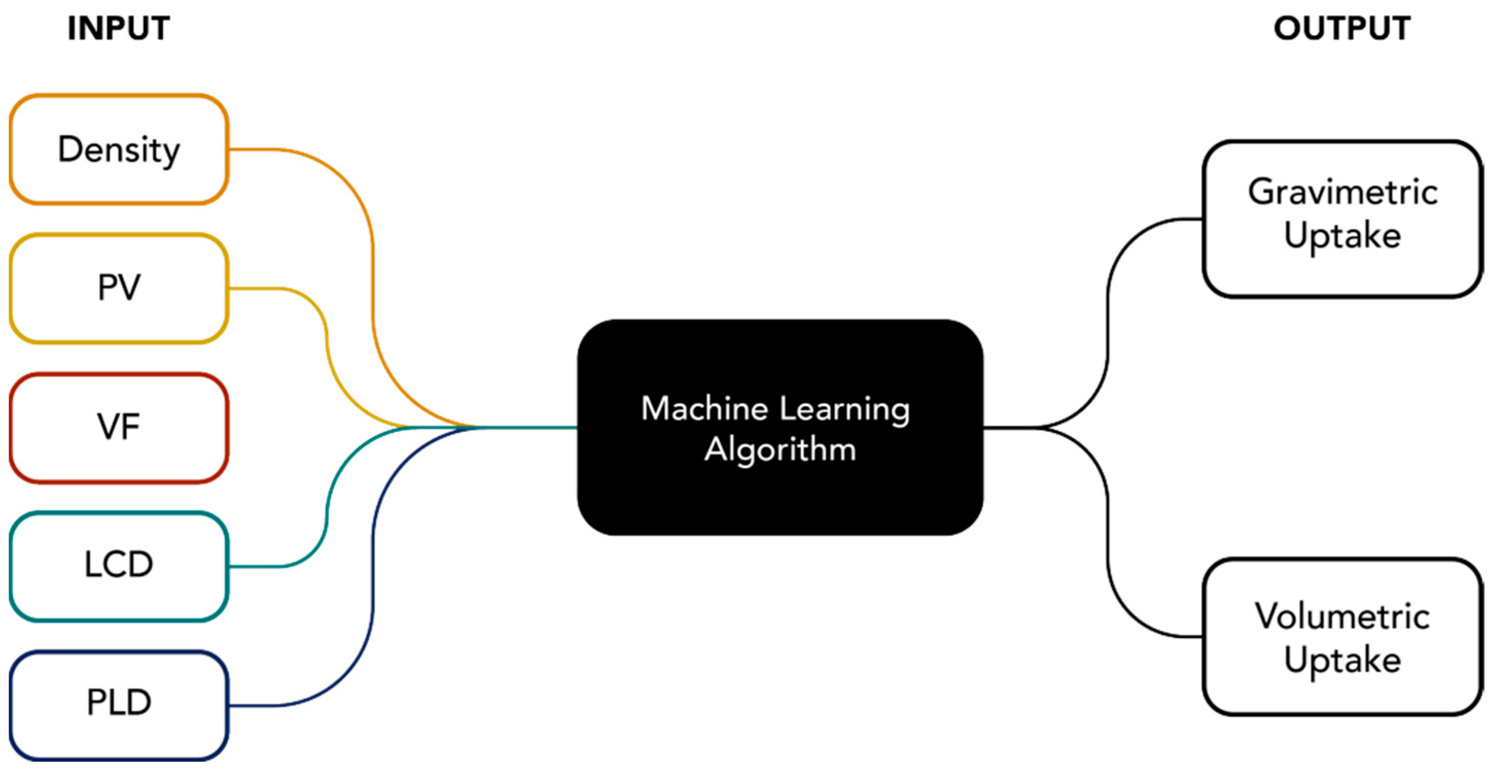
Using the data gathered, 13 machine learning methods with preset hyperparameters using MATLAB 2021b Regression Learner were tested. Five input variables were used in predicting the gravimetric uptake (UG) and volumetric uptake (UV) of hydrogen in 29,608 MOF structures. The schematic diagram of the prediction using different machine learning models is given in Figure 1.

Figure 1.
General ML schematic diagram used to predict the H2 uptake.
The five input variables and their units are enumerated in Table 2.
Table 2.
Input variables used in predicting H2 update in MOF.
The presets used for each model are enumerated in Table 3. For all the models, the ratio of the training to the testing used was 7:3. To prevent overfitting, cross-validation folds of 5 were used in all the models. In MATLAB, the model referred to as bagged tree is also the random forest model. Ahmed and Siegel pointed out the shortage of examined algorithms for H2 storage; they then addressed this shortage with the introduction of 14 different algorithms in their 2021 study. Similarly, this study opted to introduce and comparatively study algorithms not addressed in the study mentioned above. These algorithms include the quadratic support vector machine (QSVM), the Gaussian process regression (GPR) family of algorithms, and multi-layered neural networks (NNs).
Table 3.
Hyperparameters and preset values used in MATLAB regression learner.
2.3.2. Modulus Prediction
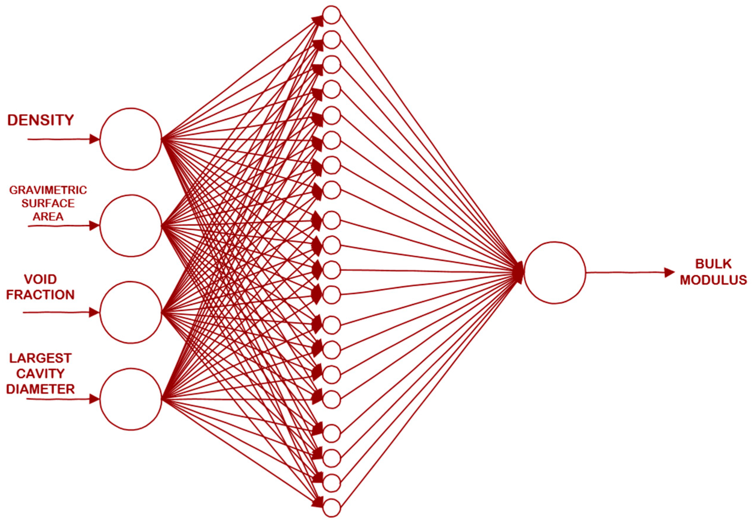
The bulk modulus was predicted using an artificial neural network that used four input variables, as enumerated in Table 4. The schematic diagram for the prediction is given in Figure 2.
Table 4.
Input variables used in predicting modulus of MOF.
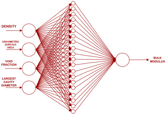
Figure 2.
Schematic diagram of the ANN generated in this study.
This ANN was trained using the Levenberg–Marquardt algorithm. The training to the testing ratio used was 7:3.
2.4. Model Performance Evaluation
The performances of the ML models were evaluated by comparing the predicted values to the GCMC simulated values and the experimental values. The following performance indicators were used: the mean squared error (MSE), coefficient of determination (R2), root mean square error (RMSE), and mean absolute error (MAE). Equation (2) shows the equation for the determination of the MSE. The MSE shows the average squared difference between the predictions and the observations that were fed to the algorithm.
Mean squared error (MSE)
Root mean square error (RMSE)
The RMSE defines the deviation between the simulated value and the actual value. It is a quantitative trade-off method. However, it becomes challenging to utilize the RMSE in the measurement of the model efficacy with differing dimensions. In this case, the coefficient of determination (R2) is also utilized to determine how well the predicted results match the actual values.
Coefficient of determination (R2)
Mean absolute error (MAE)
3. Results and Discussion
3.1. Gravimetric and Volumetric Uptakes at PS Data
The gravimetric and volumetric uptakes at the PS in the dataset used in the machine learning modeling are represented with respect to the input variables using scatter plot matrices, as shown in Figure 3 and Figure 4. The scatter plot matrices were generated using R Studio.
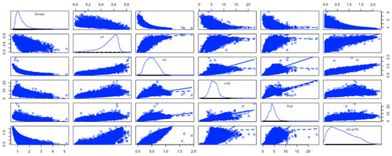
Figure 3.
Scatterplot matrix of UG at PS with respect to input variables.
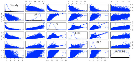
Figure 4.
Scatterplot matrix of UV at PS with respect to input variables.
The most important plots in these scatterplots are the plots in the last column. These are the pairwise relationships of the input variables with UG and UV. Some pairwise relationships are almost linear with some variability, like PV vs. UG and PLD vs. UG. All the others are nonlinear.
3.2. Evaluation of ML Models
Table 5 shows the comparison of the RMSE values for all the ML algorithms evaluated in this study. The RMSE is used as the primary performance metric for comparison due to the fact that the presentation of R2 values in MATLAB is restricted to two decimal points, leading to rounded values that are too close for comparison and even to values that are the same. For predicting the gravimetric uptakes, the best performing algorithm was found to be the tri-NN across all the performance metrics, with an RMSE value of 0.23676, closely followed by the GPR family of algorithms with RMSE values ranging from 0.285 to 0.345 for the UG uptake prediction. As for the prediction of the volumetric uptakes, the tri-NN lagged behind the GPR family of algorithms, with an RMSE of 1.874 compared to the GPR algorithm results, which ranged from 1.688 to 1.71. This result suggests that while the tri-NN suits the data for UG uptake prediction, it fails to perform well for UV uptakes.
Table 5.
Test RMSE for gravimetric (UG) and volumetric (UV) uptakes at PS.
The same trend was shown across the board, with the RMSE values differing widely between the UV and UG uptake datasets per algorithm. However, this was shown to be a notable trend across all the algorithm performances between the UV and UG uptake predictions, with the RMSE values for UV being much higher. The algorithms used all exhibited a better fit for the UG data, implying that the features used were much more relevant for the gravimetric uptakes than the UV uptakes under PS conditions and that the relationship between the input features and the output UG and UV uptakes were largely different. In any case, the data shown further reinforce the fact that the optimal choice of ML is largely problem-specific.
In general, the worst performing algorithm is the LSVM, with an RMSE value of 1.427 for UG and 5.089 for UV. This result follows the findings of Ahmed and Siegel [9], wherein the same model performed the worst among the 14 algorithms they examined. They attributed the low performance to the linear nature of the algorithms failing to fully grasp the nonlinear dependence of the multiple inputs and outputs.
3.3. H2 Uptake Prediction
To verify the reliability and accuracy of the predicted uptakes, the researchers compared the results to the experimental data taken from the benchmark study on H2 storage for MOFs under the PS conditions conducted by Garcia-Holley et al. [30], the predicted uptakes of extremely randomized trees (ERTs) used by Ahmed and Siegel [9], and the GCMC simulated results from Ahmed and Siegel. Furthermore, the accuracy of the models used in this study was compared relative to the results of the published ERT and GCMC data and experimental values. Table 6 shows the gravimetric uptakes under PS conditions obtained through the models that showed improvement compared to the ERT and GCMC data reported by Ahmed and Siegel relative to the experimental values. Low-performance algorithms are omitted from the table.
Table 6.
Comparison of H2 gravimetric uptake under PS conditions obtained through different methods.
Figure 5 shows a graphical representation of the MSE values calculated for the simulated GCMC data and ML predictions relative to the experimental UG values denoted in Table 6. The top-performing algorithm was found to be the fine tree DT variant, with an average MSE of 0.1105. To first address the discrepancy between the GCMC and predicted values, this is carried over from Ahmed and Siegel’s study [9], wherein inaccuracies in the MOF crystal structure data were cited as possible points for errors in the GCMC simulations, which directly contributed to the disagreement between the predicted and GCMC values. The remarkable results shown by the fine tree relative to the experimental values, despite the training conducted with the GCMC simulated values, are considerable and suggest that the model fit compensates for the errors incurred in the GCMC simulation.
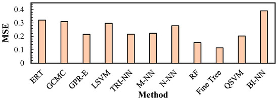
Figure 5.
MSE for gravimetric uptakes (UG) under PS conditions relative to experimental values.
From the data, it is evident that while the DT algorithm had a low score in the performance metrics for the prediction of the UG and UV uptakes in the previous section, it was able to yield values that were relatively close to the experimental benchmarks, with an MSE that was 64.5% lower than the ERT values and 63.2% lower than the GCMC values. This difference suggests that when given unseen data, this model may fare better at predicting values closer to the actual experimental values, despite the fact that the raw performance metrics were less than desirable.
Moreover, several algorithms were able to improve upon the ERT and GCMC performance in predicting the UG uptake values when compared to the experimental values. This result shows that the generated models in this study, which are easily reproducible as they require less rigorous programming, can compete with the published models in terms of accuracy.
As for UV uptake prediction, while several models improved upon the ERT performance relative to the experimental values, only the W-NN showed considerable improvement compared to both the ERT predicted values and GCMC values, as shown in Table 7 and Table 8. The W-NN predicted values with an average MSE that was less than that of the ERT values and GCMC values at 10.74. This improvement is shown in the 54% reduction in MSE relative to ERT and the 12.74% reduction relative to GCMC. Lastly, like the observations in the preceding section, the MSE values for the UV uptakes are greater across the board than the UG MSE values.
Table 7.
Comparison of H2 volumetric uptake under PS conditions obtained through different methods.
Table 8.
MSE for volumetric uptakes (UV) under PS conditions relative to experimental values.
3.4. Univariate Feature Importance
The importance of each descriptor in the ML algorithm’s predictive ability was evaluated by simulating a tri-layered NN model for UG and an exponential GPR model for UV that was developed with a single descriptor. The same ratio of 70:30 was used, splitting the data for the training and testing of these models.
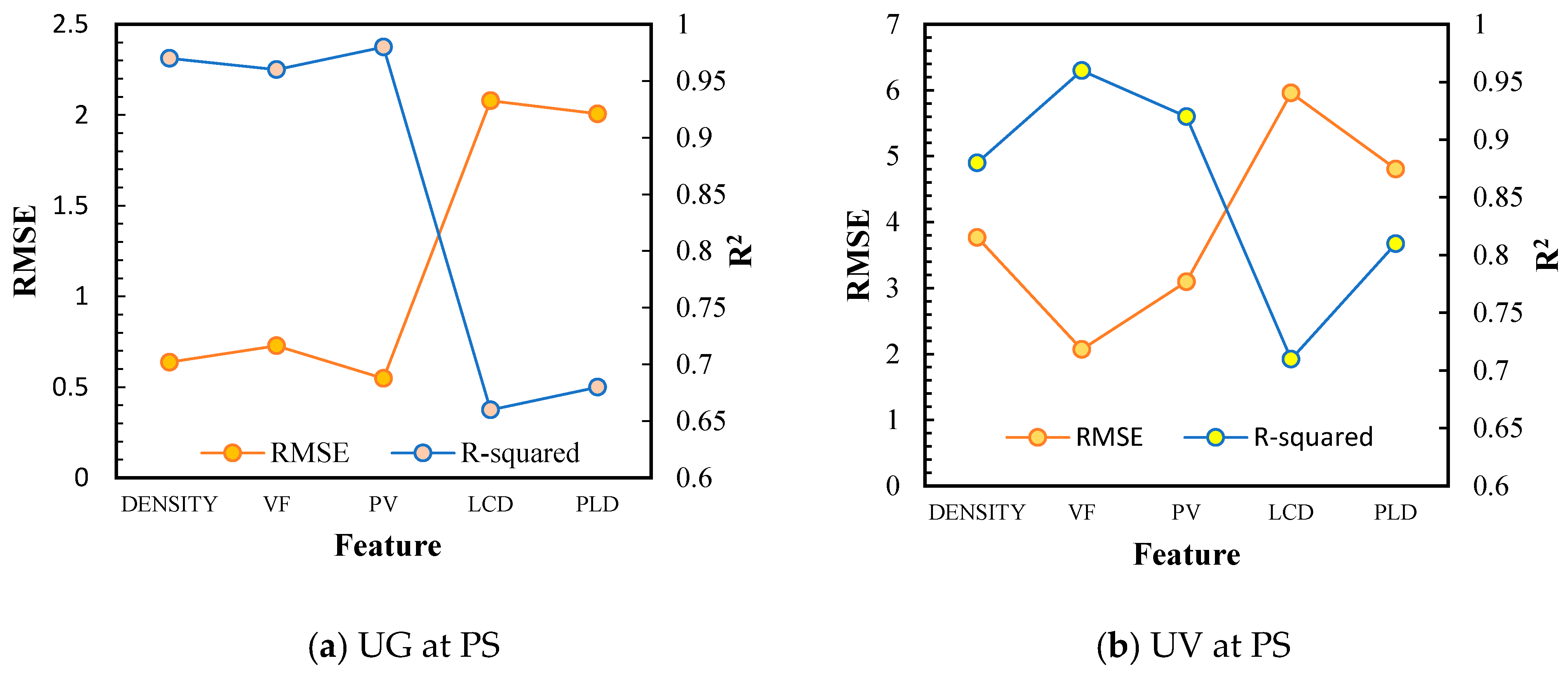
Based on Figure 6, it can be seen that the void fraction and pore volume are the two most important features that can effectively predict the MOFs’ H2 adsorptive capacity. For UG, the most crucial feature was PV, followed by density and VF. On the other hand, VF was followed by PV in terms of importance for UV. These results mirror the results reported by Ahmed and Siegel [9], who credited the significant role of pore volume to the Chahine rule. In his previous study in 2017, Ahmed [31] found that both the PV and the VF are highly correlated with the excess uptake obtained through the Chahine rule. This study by Ahmed further verifies the significance of both descriptors to the prediction.
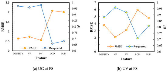
Figure 6.
Univariate feature analysis for the prediction of H2 uptake.
The hierarchy of importance for UG is as follows: PV > Density > VF > PLD > LCD. Meanwhile, the order of importance of each feature for UV prediction is as follows: VF > PV > Density > PLD > LCD. From this sequence, it can be determined that LCD was the most irrelevant feature to the prediction for both types of uptakes. Therefore, a model that was developed using only the LCD of an MOF may yield inaccurate predictions. Also, if the LCD values for the MOFs are not available within the database, one may still proceed with the conviction that the model will perform well if one possesses values for the other features, such as those used in this study or other more relevant available predictors.
On the other hand, with PV and VF being able to single-handedly produce the same accuracy as that of the model that uses all the features, it can be deduced that using these two features may prove to be enough to create a reliable and accurate model. This situation makes the model creation and data gathering procedure more straightforward and less intensive since the data for these two descriptors are usually readily available in the literature and the crystallographic data found in the databases.
3.5. Modulus Prediction
Among the ML algorithms used to predict the bulk modulus, only the created ANN was able to exceed the R2 reported by Moghadam et al. [28]. This study utilized a 4-20-1 ANN, or 4 neurons for the input layer, 20 hidden neurons for the single hidden layer, and 1 for the output layer. For easier visualization, the flow of information for the simulated ANN is shown in Figure 2.
Table 9 compares the R2 values of the simulated ANN and the ANN used in the literature. The only difference between the construction of the two ANNs was the number of hidden neurons used. The results show that the algorithm’s performance exceeds the neural network (NN) used by Moghadam et al. to predict the bulk modulus. A 9.339% increase in the coefficient of determination (R2) was observed in the simulated ANN model. This increase may be attributed to the difference in the number of hidden neurons. Shibata and Ikeda explain that the greater the number of hidden neurons present, the greater the probability of similar hidden neurons, worsening the learning performance [32]. When the learning performance worsens, it is expected that the accuracy of the predicted value compared to the actual or calculated value will be negatively affected. This concept could explain why the fit of the predicted data for the ANN in [28] is lower than this work’s ANN.
Table 9.
Comparison between the performances of ANNs in predicting the bulk modulus.
The corresponding R2 for the model indicates that the ANN could explain around 76% of the variance and that the variables used may still be quite inadequate in their ability to predict the modulus as accurately as possible [33]. However, one cannot simply add variables until the R2 becomes one because it could result in a highly complex model that might produce an overfit to the data and possibly yield poor predictions when it encounters unseen data.
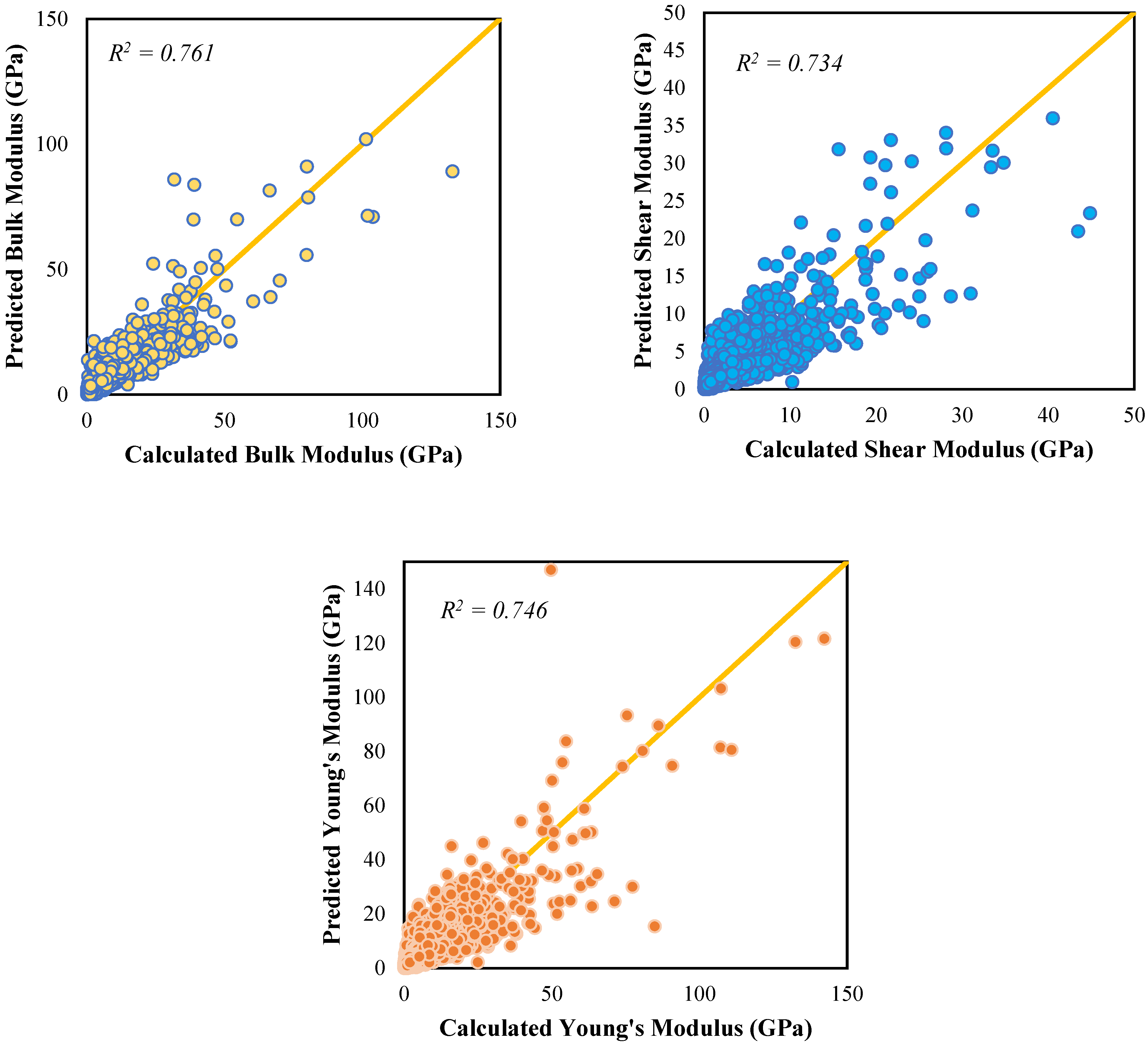
Among the other algorithms, it was also the 4-20-1 ANN that gave the most accurate prediction for the shear and Young’s moduli, respectively. Figure 7 contains the scatter plots for the predicted and calculated moduli. From the graphs, it can be noted that the ANN gave the highest R2 for the bulk modulus, which indicates that among the three moduli, the predicted bulk moduli are quite close to the bulk moduli that were computed using DFT. However, the accuracy for the shear and Young’s moduli is not very far behind.

Figure 7.
Parity plots for the fit of predicted moduli to the calculated data.
4. Future Work
As the use of hydrogen as a renewable fuel becomes increasingly viable in the future, it is important to continuously collect more data on the hydrogen uptake in different adsorbent materials, like other nanomaterials. It is also important to try different methods, like the fuzzy method [34], probabilistic methods [35,36], and deep learning methods, to increase the accuracy of the prediction of the bulk modulus of MOFs.
5. Conclusions
In this study, the researchers were able to successfully predict the gravimetric and volumetric hydrogen uptake of more than 20,000 MOFs that were obtained from several databases. Among the 13 algorithms comparatively studied, the tri-NN and GPR/E-K exhibited the best performance metrics for the UG and UV uptake prediction, respectively. The GCMC simulated and model predicted values’ reliability was verified by determining the MSE values relative to the experimental data. Afterwards, the MSE values calculated for the models utilized in this study were compared to the MSE values for GCMC and the ERT predicted values derived from Ahmed and Siegel’s study. From the comparisons made, it was found that the DT variant (fine tree) and W-NN models were able to compete with the GCMC simulated values and the ERT predicted values in terms of accuracy relative to the experimental values for the UG and UV uptakes, respectively, under PS conditions, despite their inherent simplicity. These results suggest that the top-performing models utilized in this study are viable for the prediction of the H2 storage capacities for MOFs before their synthesis to check whether the MOF can store H2 as needed by the situation.
Furthermore, the single feature importance of each of the five variables was analyzed by the generation of a tri-layered NN for UG and an exponential GPR for UV that only used a single descriptor. Through this, it was found that the pore volume and the void fraction of the MOF were indispensable yet simple features that could match the prediction fit provided by using all the features. This result simplifies the ML process and can be applied whenever there are insufficient readily available data to retrieve all the five features used in this study.
Lastly, the researchers were also able to predict the bulk, shear, and Young’s moduli of certain MOFs that were in the database of Moghadam et al. [28]. Upon using the same algorithms as those used in the uptake prediction, it was found that the 4-20-1 ANN performed the best in the prediction of the moduli. The prediction of such moduli will be relevant to the furthering of the efforts towards identifying MOFs suitable for the physisorption of hydrogen in industrial applications.
Author Contributions
Conceptualization, B.T.D.J.; methodology, N.K.B. and C.J.E.F.; software, B.T.D.J.; validation, N.K.B. and C.J.E.F.; writing—original draft preparation, N.K.B. and C.J.E.F.; writing—review and editing, B.T.D.J.; supervision, B.T.D.J.; project administration, B.T.D.J.; funding acquisition, B.T.D.J. All authors have read and agreed to the published version of the manuscript.
Funding
This research was funded by the Office of Directed Research for Innovation and Value Enhancement (DRIVE) of Mapua University.
Data Availability Statement
Data are contained within the article.
Conflicts of Interest
The authors declare no conflicts of interest.
References
- Ohno, H.; Mukae, Y. Machine Learning Approach for Prediction and Search: Application to Methane Storage in a Metal–Organic Framework. J. Phys. Chem. C 2016, 120, 23963–23968. [Google Scholar] [CrossRef]
- Thornton, A.W.; Simon, C.M.; Kim, J.; Kwon, O.; Deeg, K.S.; Konstas, K.; Pas, S.J.; Hill, M.R.; Winkler, D.A.; Haranczyk, M.; et al. Materials Genome in Action: Identifying the Performance Limits of Physical Hydrogen Storage. Chem. Mater. 2017, 29, 2844–2854. [Google Scholar] [CrossRef]
- Anderson, R.; Rodgers, J.; Argueta, E.; Biong, A.; Gómez-Gualdrón, D.A. Role of Pore Chemistry and Topology in the CO2 Capture Capabilities of MOFs: From Molecular Simulation to Machine Learning. Chem. Mater. 2018, 30, 6325–6337. [Google Scholar] [CrossRef]
- Qiao, Z.; Xu, Q.; Jiang, J. Computational screening of hydrophobic metal–organic frameworks for the separation of H2S and CO2 from natural gas. J. Mater. Chem. A 2018, 6, 18898–18905. [Google Scholar] [CrossRef]
- Dureckova, H.; Krykunov, M.; Aghaji, M.Z.; Woo, T.K. Robust machine learning models for predicting high CO2 working capacity and CO2/H2 selectivity of gas adsorption in metal organic frameworks for precombustion carbon capture. J. Phys. Chem. C 2019, 123, 4133–4139. [Google Scholar] [CrossRef]
- Wu, X.; Xiang, S.; Su, J.; Cai, W. Understanding Quantitative Relationship between Methane Storage Capacities and Characteristic Properties of Metal-Organic Frameworks Based on Machine Learning. J. Phys. Chem. C 2019, 123, 8550–8559. [Google Scholar] [CrossRef]
- Bucior, B.J.; Bobbitt, N.S.; Islamoglu, T.; Goswami, S.; Gopalan, A.; Yildirim, T.; Farha, O.K.; Bagheri, N.; Snurr, R.Q. Energy-based descriptors to rapidly predict hydrogen storage in metal-organic frameworks. Mol. Syst. Des. Eng. 2019, 4, 162–174. [Google Scholar] [CrossRef]
- Samantaray, S.S.; Putnam, S.T.; Stadie, N.P. Volumetrics of hydrogen storage by physical adsorption. Inorganics 2021, 9, 45. [Google Scholar] [CrossRef]
- Ahmed, A.; Siegel, D.J. Predicting hydrogen storage in MOFs via machine learning. Patterns 2021, 2, 100291. [Google Scholar] [CrossRef]
- Safaei, M.; Foroughi, M.M.; Ebrahimpoor, N.; Jahani, S.; Omidi, A.; Khatami, M. A review on metal-organic frameworks: Synthesis and applications. TrAC-Trends Anal. Chem. 2019, 118, 401–425. [Google Scholar] [CrossRef]
- Petit, C. Present and future of MOF research in the field of adsorption and molecular separation. Curr. Opin. Chem. Eng. 2018, 20, 132–142. [Google Scholar] [CrossRef]
- Li, J.R.; Kuppler, R.J.; Zhou, H.C. Selective gas adsorption and separation in metal-organic frameworks. Chem. Soc. Rev. 2009, 38, 1477–1504. [Google Scholar] [CrossRef]
- Taylor, M.K.; Runčevski, T.; Oktawiec, J.; Gonzalez, M.I.; Siegelman, R.L.; Mason, J.A.; Ye, J.; Brown, C.M.; Long, J.R. Tuning the Adsorption-Induced Phase Change in the Flexible Metal-Organic Framework Co(bdp). J. Am. Chem. Soc. 2016, 138, 15019–15026. [Google Scholar] [CrossRef]
- Li, H.; Wang, K.; Sun, Y.; Lollar, C.T.; Li, J.; Zhou, H.C. Recent advances in gas storage and separation using metal–organic frameworks. Mater. Today 2018, 21, 108–121. [Google Scholar] [CrossRef]
- Lin, X.; Jia, J.; Champness, N.R.; Hubberstey, P.; Schröder, M. Metal-organic framework materials for hydrogen storage, Solid-State Hydrog. Storage Mater. Chem. 2008, 288–312. [Google Scholar] [CrossRef]
- Tian, T.; Zeng, Z.; Vulpe, D.; Casco, M.E.; Divitini, G.; Midgley, P.A.; Silvestre-Albero, J.; Tan, J.C.; Moghadam, P.Z.; Fairen-Jimenez, D. A sol-gel monolithic metal-organic framework with enhanced methane uptake. Nat. Mater. 2018, 17, 174–179. [Google Scholar] [CrossRef] [PubMed]
- Pascanu, V.; Miera, G.G.; Inge, A.K.; Martín-Matute, B. Metal-Organic Frameworks as Catalysts for Organic Synthesis: A Critical Perspective. J. Am. Chem. Soc. 2019, 141, 7223–7234. [Google Scholar] [CrossRef] [PubMed]
- Farrusseng, D.; Aguado, S.; Pinel, C. Metal-organic frameworks: Opportunities for catalysis. Angew. Chem.-Int. Ed. 2009, 48, 7502–7513. [Google Scholar] [CrossRef] [PubMed]
- Wang, Q.; Astruc, D. State of the Art and Prospects in Metal-Organic Framework (MOF)-Based and MOF-Derived Nanocatalysis. Chem. Rev. 2020, 120, 1438–1511. [Google Scholar] [CrossRef] [PubMed]
- De Wu, C. Crystal Engineering of Metal-Organic Frameworks for Heterogeneous Catalysis. In Selective Nanocatalysts and Nanoscience: Concepts for Heterogeneous and Homogeneous Catalysis; John Wiley & Sons: Hoboken, NJ, USA, 2011; pp. 271–298. [Google Scholar] [CrossRef]
- Rajoub, B. Supervised and unsupervised learning. In Biomedical Signal Processing and Artificial Intelligence in Healthcare; Academic Press: Cambridge, MA, USA, 2020; pp. 51–89. [Google Scholar] [CrossRef]
- Chong, S.; Lee, S.; Kim, B.; Kim, J. Applications of machine learning in metal-organic frameworks. Coord. Chem. Rev. 2020, 423, 213487. [Google Scholar] [CrossRef]
- Seko, A. Descriptors for machine learning of materials data. arXiv 2017, arXiv:1709.01666. [Google Scholar]
- Luna, A.S.; Alberton, K.P.F. Applications of artificial neural networks in chemistry and chemical engineering. Artif. Neural Netw. New Res. 2017, 17, 25–44. [Google Scholar]
- Tsamardinos, I.; Fanourgakis, G.S.; Greasidou, E.; Klontzas, E.; Gkagkas, K.; Froudakis, G.E. An Automated Machine Learning architecture for the accelerated prediction of Metal-Organic Frameworks performance in energy and environmental applications. Microporous Mesoporous Mater. 2020, 300, 110160. [Google Scholar] [CrossRef]
- Pardakhti, M.; Moharreri, E.; Wanik, D.; Suib, S.L.; Srivastava, R. Machine Learning Using Combined Structural and Chemical Descriptors for Prediction of Methane Adsorption Performance of Metal Organic Frameworks (MOFs). ACS Comb. Sci. 2017, 19, 640–645. [Google Scholar] [CrossRef] [PubMed]
- Deng, X.; Yang, W.; Li, S.; Liang, H.; Shi, Z.; Qiao, Z. Large-scale screening and machine learning to predict the computation-ready, experimental metal-organic frameworks for CO2 capture from air. Appl. Sci. 2020, 10, 569. [Google Scholar] [CrossRef]
- Moghadam, P.Z.; Rogge, S.M.J.; Li, A.; Chow, C.M.; Wieme, J.; Moharrami, N.; Aragones-Anglada, M.; Conduit, G.; Gomez-Gualdron, D.A.; Van Speybroeck, V.; et al. Structure-Mechanical Stability Relations of Metal-Organic Frameworks via Machine Learning. Matter 2019, 1, 219–234. [Google Scholar] [CrossRef]
- Ren, J.; North, B. Shaping Porous Materials for Hydrogen Storage Applications: A Review. J. Technol. Innov. Renew. Energy 2014, 3, 12–20. [Google Scholar] [CrossRef]
- Paula García-Holley, O.K.F.; Schweitzer, B.; Islamoglu, T.; Liu, Y.; Lin, L.; Rodriguez, S.; Weston, M.H.; Hupp, J.T.; Gómez-Gualdrón, D.A.; Yildirim, T.; et al. Benchmark Study of Hydrogen Storage in Metal−Organic Frameworks under Temperature and Pressure Swing Conditions. ACS Energy Lett. 2018, 3, 748–754. [Google Scholar] [CrossRef]
- Ahmed, A.; Liu, Y.; Purewal, J.; Tran, L.D.; Wong-Foy, A.G.; Veenstra, M.; Matzger, A.J.; Siegel, D.J. Balancing gravimetric and volumetric hydrogen density in MOFs. Energy Environ. Sci. 2017, 10, 2459–2471. [Google Scholar] [CrossRef]
- Shibata, K.; Ikeda, Y. Effect of Number of Hidden Neurons on Learning in Large-Scale Layered Neural Networks; ICCAS-SICE: Fukuoka, Japan, 2009; pp. 5008–5013. [Google Scholar]
- Miles, J. R-Squared, Adjusted R-Squared. In Encyclopedia of Statistics in Behavioral Science; John Wiley & Sons: Hoboken, NJ, USA, 2005. [Google Scholar] [CrossRef]
- Ardabili, S.F.; Najapi, B.; Shamshirband, S. Fuzzy Logic Method for the prediction of Cetane Number using Carbon Number, Double Bounds, Iodic, and Saponification Values of Biodiesel Fuels. Environ. Prog. Sustain. Energy 2019, 38, 584–599. [Google Scholar] [CrossRef]
- Zhang, Y.; Wang, H.; Mao, J. Probabilistic Framework with Bayesian Optimization for Predicting Typhoon-Induced Dynamic Responses of a Long-Span Bridge. J. Struct. Eng. 2021, 147, 04020297. [Google Scholar] [CrossRef]
- Zhang, Y.-M.; Wang, H. Multi-Head Attention-Based Probabilistic CNN-BiLSTM for Day-Ahead Wind Speed Forecasting. Energy 2023, 278, 127865. [Google Scholar] [CrossRef]


Disclaimer/Publisher’s Note: The statements, opinions and data contained in all publications are solely those of the individual author(s) and contributor(s) and not of MDPI and/or the editor(s). MDPI and/or the editor(s) disclaim responsibility for any injury to people or property resulting from any ideas, methods, instructions or products referred to in the content. |
© 2024 by the authors. Licensee MDPI, Basel, Switzerland. This article is an open access article distributed under the terms and conditions of the Creative Commons Attribution (CC BY) license (https://creativecommons.org/licenses/by/4.0/).