Optimizing the Journey: Dynamic Charging Strategies for Battery Electric Trucks in Long-Haul Transport

Abstract

Battery electric trucks (BETs) represent a well-suited option for decarbonizing road freight transport to achieve climate targets in the European Union. However, lower ranges than the daily distance of up to 700 km make charging stops mandatory. This paper presents an online algorithm for optimal dynamic charging strategies for long-haul BET based on a dynamic programming approach. In several case studies, we investigate the advantages optimal strategies can bring compared to driver decisions. We further show which charging infrastructure characteristics in terms of charging power, density, and charging station availability should be achieved for BETs in long-haul applications to keep the additional time required for charging stops low. In doing so, we consider the dynamic handling of occupied charging stations for the first time in the context of BET. Our findings show that, compared to driver decisions, optimal charging strategies can reduce the time loss by half compared to diesel trucks. To keep the time loss compared to a diesel truck below 30 min a day, a BET with a 500 kWh battery would need a charging point every 50 km on average, a distributed charging power between 700 and 1500 kW, and an average charger availability above 75%. The presented method and the case studies’ results’ plausibility are interpreted within a comprehensive sensitivity analysis and subsequently discussed in detail. Finally, we transformed our findings into concrete recommendations for action for the efficient rollout of BETs in long-haul applications.

1. Introduction

The transport sector is responsible for 26% of global greenhouse gas (GHG) emissions in Europe [1]. The decarbonization of this sector is imperative to achieve the EU goal of climate neutrality by 2050 [2]. In addition to increasingly stringent EU CO₂ targets with a reduction of 30% by 2030 for truck original equipment manufacturers (OEM), customers are also demanding the possibility of zero-emission vehicles (ZEV) [3]. This is influenced by the mandatory disclosure of the sustainability report for industry companies following the European Sustainability Reporting Standards (ERSR) from 2025 onwards [4]. Battery electric trucks (BET) represent an opportunity for reducing emissions and, with a well-to-wheel efficiency of about 75%, offer the highest efficiency compared to other ZEV powertrain designs using hydrogen or synthetic fuels as an energy source [5,6]. Therefore, several truck OEMs [7,8,9] have heavy-duty BET in their portfolio or have announced them for the following years and expect a corresponding market ramp-up [10]. Alongside BETs, charging infrastructure operators are currently pushing into the market [11,12].

Several research studies show BETs’ feasibility [13,14,15,16] and economic competitiveness [17,18,19] compared to today’s diesel trucks. Previous work in the BET context deals with the topics of battery dimensioning [17,20,21] and cell selection [18,20,22]. However, the BET range that can be achieved while meeting payload and installation space requirements is currently insufficient for long-haul transport with daily ranges up to 700 km without intermediate on-route charging [20].

Several studies [14,17,19,20] investigate the influence of these intermediate fast-charging events with different charging powers on the battery dimensioning, cell selection, and TCO. For this purpose, either synthetic scenarios [14,17,20] based on the hour of service (HoS) regulations applicable in the EU [23] or an explicit route with defined stops for the charging events are used [19]. Only a few studies investigate the required charging infrastructure for BET. Speth et al. [24] present a model for public charging infrastructure based on traffic census data and the resulting charging demand. To determine the number of chargers per charging point, they use a queuing model to allocate vehicles to individual charging stations. Auer et al. [25] evaluate current rest stops in Germany for their suitability as charging points for BET. For this evaluation, they use different input data sets, such as truck stop locations, and extend them with specific data, such as grid connection or land use. However, no evaluation is made from the driver’s perspective. Hecht et al. [26] show such an evaluation in the context of battery electric passenger vehicles (BEV) for a charging network in Germany based on the resulting time loss due to required charging stops. Based on precalculated routes, they show a two-level approach for planning charging stops by first identifying all feasible chargers along the route. Subsequently, the amount of recharged energy is optimized.

The search for charging points in different contexts has also been intensively studied as part of the electric vehicle routing problem (EVRP) with its several formulations [27]. Our previous work presented a comprehensive review of the existing state-of-the-art methodologies for solving this problem [28]. Sweda et al. [29] consider uncertain, occupied charging stations for the first time. They used a dynamic programming approach to solve the formulated multi-stop shortest path problem. Guillet et al. [30] show a real-time rollout algorithm that finds optimal decisions on the fly, such as whether to wait or pass in case of an occupied charging station. However, the presented research does not consider the mandatory rest times applicable in the truck domain, which must be considered when planning the charging stops. Furthermore, only Hecht et al. [26] consider the real charging behavior of BEVs, i.e., the charging power reduction in a high state of charge (SOC).

To the best of our knowledge, only Bai et al. [31] show an approach for optimal charging stop planning specifically for BET and the related consideration of mandatory rest times. They present a powerful algorithm for the online calculation of charging strategies but neglect the possibility of dividing the rest into 15 and 30 min. Following this, no realistic battery-charging behavior is modeled due to the formulation of a linear optimization problem. Bai et al. [31] base their investigation on a charging infrastructure network in Sweden and corresponding precalculated routes. Our works differ both in the implemented algorithm to overcome the simplifications assumed by Bai et al. [31] and in the scope. We specify our contribution in the next section.

1.1. Contribution

The battery’s real charging behavior strongly influences the optimal planning of the charging stops. Due to the decreasing charging power for high SOC ranges, shorter stops in the medium SOC range could be advantageous in terms of time. Also, due to the allowed break split of 15 and 30 min, the driving time model gives room for exactly such optimizations, which are not considered in previous work. Our method supports an online strategy analogous to that of Bai et al. [31]. We integrate the charging strategy into a holistic framework for simulating long-haul transportation scenarios with BET. Previous work studying battery size and required charging power uses synthetic scenarios for both driving cycles and charging events. Here, we use real-world driving data to create driving cycles and the presented charging strategy to evaluate the battery size and, especially, charging infrastructure characteristics under nearly real conditions for the first time. Based on this, our article provides concrete recommendations for action for the rollout of the charging infrastructure for BET. The research goals can be summarized as follows:

• Proposing an online algorithm for a dynamic charging strategy and corresponding framework for the operation simulation of BET:
  This paper proposes the first optimal online charging strategy considering real charging behavior and rest regulations. The proposed strategy can also handle real-world charging station behavior, such as occupation. We propose an open-source simulation framework for battery electric trucks, including vehicle, infrastructure, and operation simulation models, where we include the proposed strategy. This framework can be used for the simultaneous design of the BET and of the public charging infrastructure.
• Simulative case studies to outline recommendations of action for the efficient rollout of BET in long-haul applications:
  We use the proposed framework and charging strategy to first investigate the dependencies between truck and charging infrastructure properties. Second, we show which rollout of charging infrastructure is sufficient to ensure the operability of BET. For this, we use three case studies that address the following three research questions:

  (a)

  How do battery capacity and available charging power influence the operation time of BET in long-haul applications?

  (b)

  For today’s BET, which infrastructure properties of charger density and charging power should be applied?

  (c)

  How does real-world charging station behavior, such as occupation, change these fundamental requirements?

1.2. Article Organization

This article is organized as follows. Section 2 first shows the underlying problem description and the mathematical problem formulation of finding optimal charging stops before proposing a solution approach. Section 3 shows the parametrization of the implemented simulation framework followed by its application in three different case studies and integration levels of real-world charging infrastructure properties in Section 4. Section 5 shows a comprehensive sensitivity analysis of the most relevant parameters. We close this research article with a discussion in Section 6 and a brief outlook on future work in Section 7.

2. Method

To show our method of finding optimal on-route charging stops for BETs, we start with an abstract problem description followed by its mathematical formulation.

2.1. Problem Description

Due to installation space limitations, BETs have shorter ranges than those that fulfill the transport task in long-haul transport without a charging stop [20]. Typical daily driving distances in long-haul transport are between 650 and 700 km [32]. When integrating charging stops, the applicable HoS regulations must be considered. This means the driver has to rest for 45 min after a driving period of 4.5 h at the latest. However, the rest time may be divided into a 15 min break followed by a 30 min break. [23]. On an abstract level, the problem of integrating optimal charging stops can be formulated as follows: A given route and its velocity profile with a set of upcoming points of interest (POI), e.g., charging stations, is to be completed with the lowest cost while respecting the rest time regularities and the battery SOC limits. Costs can be time, calculated total cost of ownership, or a mix of both. Therefore, several properties of this problem are considered within optimization. The energy needed to drive from one POI to the next one is pre-calculated based on a quasistatic longitudinal simulation of the considered route. We consider non-linear charging and pre-calculate charging maps as look-up tables for realistic behavior. We show these in detail in Section 3. The mathematical optimization problem is described in the next section, followed by the proposed solution algorithm.

2.2. Mathematical Problem Formulation

For the solution to the problem considered here, we assume that the vehicle’s velocity is given and is not considered as part of the optimization problem described below.

Let $R$ be a route with the POI $r_i,\left(i=0,\dots ,n-1\right)$ and the destination $r_n$. Further, let $\mathit{t}=\left[t_0, t_1,\dots ,t_{n-1}\right]$ be the vector with the total idle time $t_i$ at each POI, $r_j$ the furthest POI, that can be reached within the allowed driving time of 4.5 h, and $C_i$ the cost of stopping and charging at POI $r_i$. The optimal idle times ${\mathit{t}}_{opt}$ are found by solving (1).

$${\mathit{t}}_{opt}=\arg \min \left({\displaystyle \sum }_{i=0}^{n-1}{C}_i\right)$$

(1)

The cost $C_i$ of a stop can include both temporal and monetary aspects, such as the charging costs. However, in this article, we formulate the cost as the total time the truck spends at a certain POI. The idle time $t_i$ at POI $r_i$ results from the maximum of the charging time $t_{i,ch}\in {ℝ}_0^{+}$ and the rest time $t_{i,r}\in \left\{0, 15, 30, 45 \min \right\}$ spent at this POI. While the charging time only has to be greater or equal to zero, the rest time is discretized according to the HoS regulations [23].

$$\begin{gathered} C_i=t_i \\ \mathrm{with} t_i=\max \left(t_{i,ch},t_{i,r}\right) \end{gathered}$$

(2)

The optimization problem (1) is further constrained by (3)–(5).

$$\begin{gathered} {\displaystyle \sum }_{i=0}^{i=j}{t}_{i,r}\ge 45 \min \\ \mathrm{with} r_j \mathrm{as} \mathrm{the} \mathrm{POI}, \mathrm{for} \mathrm{which} \mathrm{the} \mathrm{following} \mathrm{holds}:{\displaystyle \sum }_{i=0}^{i=j}{t}_{dr,i,i+1}\le 4.5 \mathrm{h} \end{gathered}$$

(3)

$$\begin{gathered} t_m\ge 30 \min \\ \mathrm{with} m=\max \left\{i|0\le i\le j \mathrm{and} t_i>0\right\} \end{gathered}$$

(4)

$${\mathrm{soc}}_{\max }\ge {\mathrm{soc}}_{\mathrm{i}}\ge {\mathrm{soc}}_{\min }, \mathrm{i}=0,\dots ,\mathrm{n}$$

(5)

C1 (3) and C2 (4) ensure compliance with the HoS regulations in Europe [23], where $t_{dr,i,i+1}$ is the predicted driving time from POI $r_i$ to $r_{i+1}$ and $r_j$ is the POI, that can furthest be reached within 4.5 h driving time (Figure 1).

The constraints C1 (3) and C2 (4) can be neglected for trips with a predicted driving time below 4.5 h. C3 (5) specifies the truck battery’s minimum SOC $so{c}_{min}$. The energy consumption between two POIs is calculated through a longitudinal dynamic simulation based on the prescribed velocity profile. The presented optimization problem has crucial properties for application in the vehicle, which influence the choice of a solution approach.

2.3. Properties of the Considered Problem

Before proposing a solution procedure, we first want to provide the reason for needing a dynamic strategy. Two key aspects can show this. First, the required travel time must be predicted to identify the critical POI $r_j$. This prediction is subject to uncertainty due to real-world effects such as congestion. Due to the increasing time horizon, it can be assumed that the prediction becomes worse as the distance of the POI from the current position increases. Second, SOC or energy consumption prediction is required to satisfy (5). This will also be subject to uncertainties in real-world applications. In addition to the technical uncertainties in the prediction, there is a practical uncertainty in the availability of charging points. Charging points may be occupied upon arrival. We assume such information will be available in the future; so, historical data can be used to output probabilities of such occupancy and expected waiting times $t_{i,w}$ at a specific POI $r_i$.

Due to the presented properties of the problem formulation in real-world applications, global optimization methods are less suitable since they determine the overall optimal solution ${\mathit{t}}_{opt}$ before the start of the trip. Consequently, they cannot consider the mentioned uncertainties during the trip. We, therefore, soften the global optimal solution and find the situational optimal solution for each POI $r_i$ along route R when the BET reaches that POI. We refer to this as a dynamic charging strategy since the required predictions are updated again at each POI, and consequently, dynamic effects can be considered.

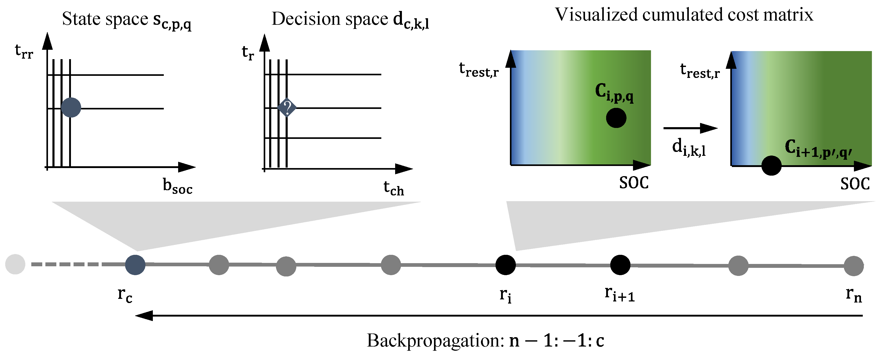
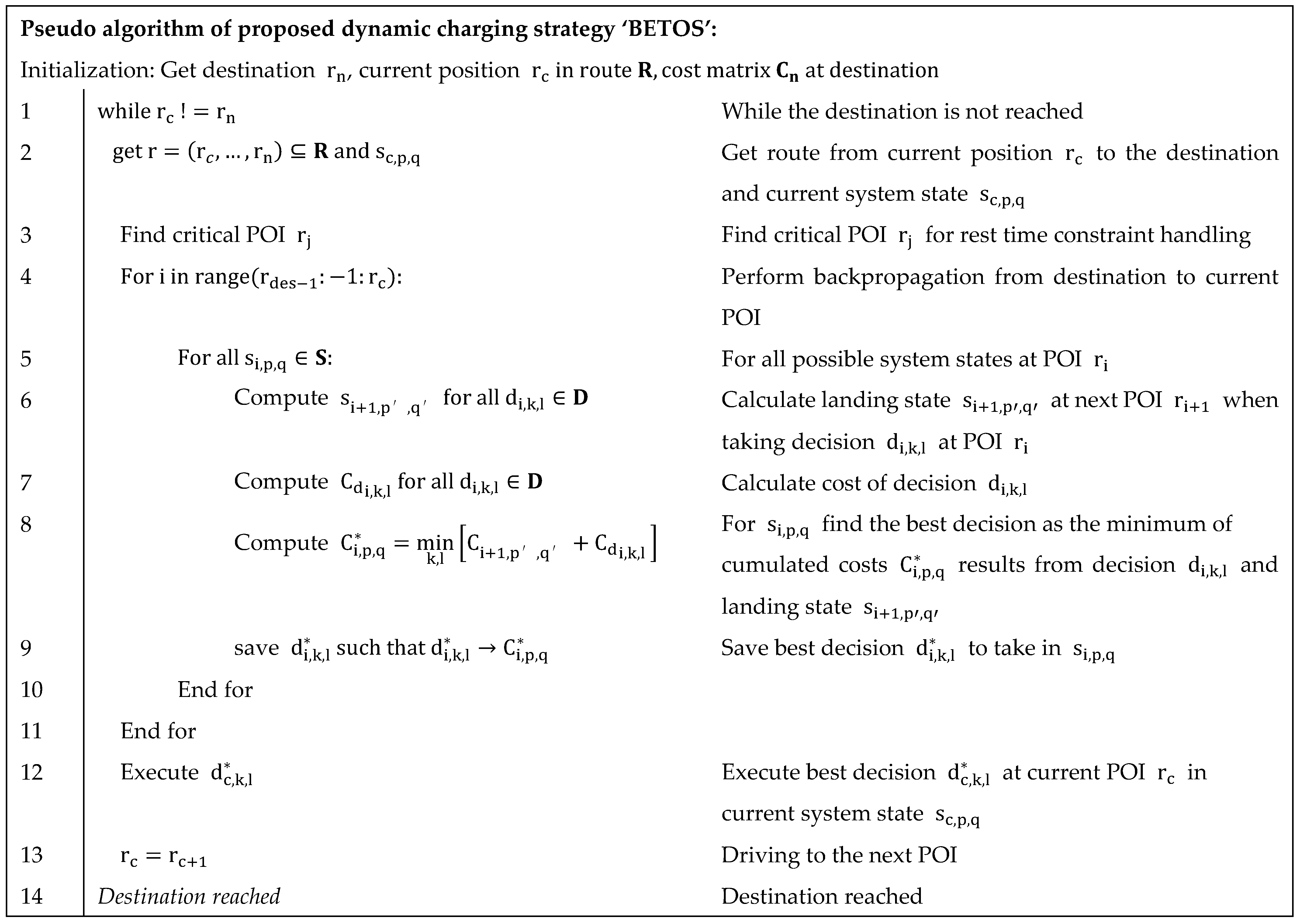
2.4. Solution Approach: Dynamic Programming

We use a dynamic programming (DP) approach to solve the respective situational optimization problem. This approach proved to be an efficient solution method for this type of problem in the context of EVRP [33,34].

For using DP, we first define the system state. To handle the constraints of C1 to C3, a system state $s_{i,p,q}$ described by three variables is used. A state is thus defined by the POI $r_i$, the trucks SOC $b_{soc,p}$ on arrival at this POI $r_i$ and the remaining rest time $t_{rr,q}$ the driver has to perform according to the HoS regulation [23].

$$s_{i,p,q}=\left[r_i,b_{soc,p},t_{rr,q}\right]$$

(6)

We discretize the battery’s SOC in one percent steps. The discretization of the remaining rest time can be derived directly from the HoS regulations [23]. Accordingly, the remaining rest time is either zero, 30 min if one part of the total rest time is done, or 45 min if no rest is performed. The state of 15 min for the remaining rest time is not allowed since the second the rest split has to be 30 min at a minimum [23].

$$b_{soc,p}\in \left[0,0.01, \dots , 1\right], t_{rr,q} \in \left[0, 30, 45\right] \min$$

(7)

The advantage of using the remaining rest time $t_{rr}$ to be completed is the reduction to three possible states instead of using the already completed rest time, which would require four states (0, 15, 30 and 45 min). The decisions a driver could take at POI $r_i$ are the charging time $t_{ch}$ and the rest time $t_r$. Therefore, we combine these into the decision space $d_{i,k,l}$.

$$d_{i,k,l}=\left[r_i,t_{ch,k}, t_{r,l}\right]$$

(8)

The charging time is discretized in one-minute steps with a maximum charging time of 100 min. Analogously to the state space, the decisions in terms of rest time are derived from the HoS regulations [23]. We incorporate the allowed rest split of 15 and 30 min here.

$$t_{ch,k}\in \left[0,1,2,\dots ,100\right] \min , t_{r,l}\in \left[0,15,30,45\right] \min$$

(9)

To find the best situational decision to take at POI $r_i$, we perform backward propagation by using the following recursive formula based on the defined cost at the destination $C_n$.

$$\begin{array}{r}{C}_{i,p,q}=\underset{k,l}{\min }\left(C_{d_{i,k,l}}+C_{i+1,p^{\prime },q^{\prime }}\right)\\ \mathrm{with} s_{i,p,q}\stackrel{d_{i,k,l}}{\to }{s}_{i+1,p^{\prime },q^{\prime }}\end{array}$$

(10)

The best decision to take at POI $r_i$ when arriving in state $s_{i,p,q}$ is decision $d_{i,k,l}$, which minimizes the sum of the decision cost $C_{d_{i,k,l}}$ and the cumulated cost $C_{i+1,p^{\prime },q^{\prime }}$ of the state $s_{i+1,p^{\prime },q^{\prime }}$ which results from taking decision $d_{i,k,l}$. The discretization of the SOC $b_{soc,p}$ (8) and the charging time $t_{ch,k}$ (9) are hyperparameters that determine the computation time and accuracy of the solution. However, the discretization of the remaining rest time $t_{rr,q}$ (8) and the chosen rest time $t_{r,l}$ (9) result from the rest regulations in EU. The non-linear charging behavior of the BET is taken into account via the charging time selected. Depending on the SOC at the start of a charging process (indices p in system state), the same charging time leads to a different increase in SOC through the charging session. Figure 2 visualizes the proposed approach to find the situational optimal decision at an upcoming POI $r_c$ based on backpropagation. In this article, we will abbreviate the presented charging strategy as Battery Electric Truck Operation Strategy (BETOS). Figure 3 shows its implementation as a pseudo-code based on the mathematical solution shown.

When the truck reaches the position of the upcoming POI $r_c$, the optimal decision $d_{c,k,l}^{*}$ is made based on the current SOC $b_{soc,p}$ and the remaining rest time $t_{rr,q}$ (leading to the system state $s_{c,p,q}$). First, the critical POI $r_j$ regarding the legal driving period is identified (L3). The critical POI ${\mathrm{r}}_{\mathrm{j}}$ is the POI that can just be reached within the remaining driving time based on the current system state. Based on this, the cost matrix for the POI $r_{j+1}$ after the critical one is manipulated so that the remaining rest time $t_{rr}$ has to be zero at the POI $r_{j+1}$ (Figure 1). This allows the best decision (L9) for the upcoming POI $r_c$ to be found recursively starting from the destination (L4) based on the resulting minimum cumulative cost (L5–8). Finally, the best decisions $d_{c,k,l}^{*}$ can be executed at the upcoming POI $r_c$ (L12). The BETOS algorithm shown is integrated into a simulation framework based on [28], in which the driving to the next POI is performed in a longitudinal driving simulation (L13). The procedure repeats at each POI until the destination is reached (L1). Therefore, the position of the critical POI is also checked and recalculated at each POI. In this way, dynamic effects such as traffic jams and the possibility that the second driving interval takes longer than 4.5 h can be considered.

We want to look closely at one line of the pseudo-code, which is essential for the following chapters. In L6, for an assumed state $s_{i,p,q}$ and a decision $d_{i,k,l}$, the resulting state $s_{i+1,p^{\prime },q^{\prime }}$ at the next POI is calculated. We use a quasistatic longitudinal dynamics simulation for predicting the energy consumption between two POIs $r_i$ and $r_{i+1}$ due to the significantly faster computation time than the forward simulation used in the framework shown below. The disadvantage of assuming the exact following of a given velocity profile leads to some prediction errors in energy consumption. We will examine such deviations in more detail in Section 5, where we investigate their sensitivity. In the next paragraph, we show the simulation framework, particularly its parametrization, before we apply the proposed algorithm to different case studies.

3. Simulation Framework and Parametrization

The simulation framework used here, in which BETOS is embedded, includes a vehicle and infrastructure model [28]. A forward simulation lets the vehicle drive a given driving cycle. The charging management module determines the interaction between the vehicle and the charging infrastructure. The forward simulation and the vehicle model will not be further discussed here. A detailed setup can be found in the previous work [28]. The parameters used for all simulation models are shown in Appendix A. In the following section, we show the most relevant parameters of the models and go into more detail about the infrastructure model.

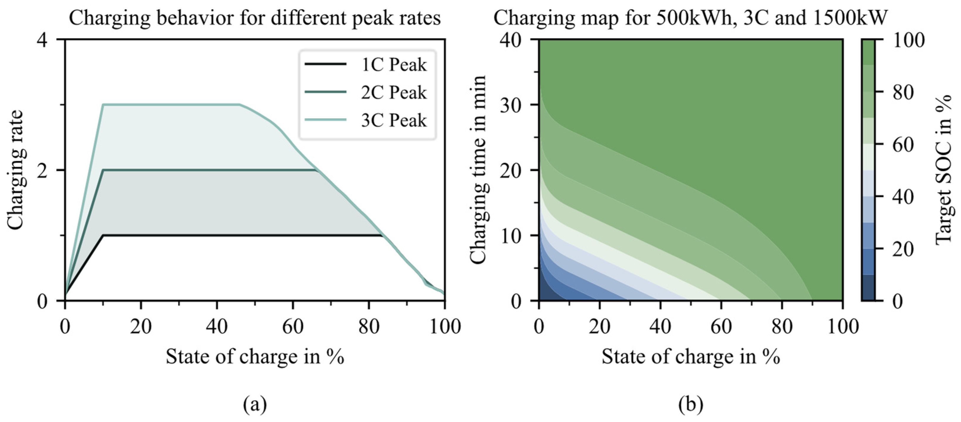
3.1. Model Parametrization

On the vehicle side, the charging behavior has the most significant influence on the charging strategy. We assume the SOC-dependent charging behavior shown in Figure 4a [35]. The dependencies on the battery temperature or the State of Health (SOH) of the battery are not considered here. To reduce the computation time of the charging strategy algorithm, we pre-calculate charging maps from the behavior shown, which reflects the SOC after the charging process for a selected charging time and starting SOC. An exemplary charging map for an available charging power of 1500 kW and an allowed charging rate of 3 C are shown in Figure 4b. These lookup tables consider the non-linear charging behavior and are used within the DP approach. To pre-calculate these maps, for every considered charging time, possible starting SOC, and available charging power, the resulting SOC after the charging event is estimated for a specific battery capacity using the power profiles from Figure 4a.

The infrastructure model is based on the transportation scenario, given by a driving cycle and a payload. Here, the payload is set constant to 19.3 t, mandatory for type approval in the EU [36,37]. For the derivation of the driving cycles, microtrips were extracted from recorded truck mobility data [32], i.e., driving sections with zero vehicle speed at the beginning and end [38]. For the long-haul context considered here, these microtrips are combined into tours totaling 650 to 700 km. Along such a driving cycle, POIs are placed by the infrastructure model. Initially, at each end of a microtrip, a POI is placed. Between two POIs defined by this, further POIs are defined. The number depends on the density in POI per 100 km prescribed. In the second step, each POI is assigned a charging power. Both parameters, density and power, can be constant or follow a distribution. Figure 5 shows a created driving cycle from microtrips and the placed POIs.

We model the charging infrastructure using the synthetic parameters for two reasons. First, no real charging infrastructure networks for BET exist today. Second, we want to use the parameters to identify concrete recommendations for action on how charging infrastructure for BET should be set up. In contrast to previous approaches of infrastructure planning for BET, which are based on traffic data [24,25], we show the driver’s perspective to outline what properties are desirable. The charging strategy determines the interaction of the BET and the infrastructure in the simulation. The next section shows the parametrization for the following case study analysis.

3.2. Strategy Parametrization

For a better classification of the application of the proposed simulation framework shown in the next chapter, we compare the effects of the decisions using the presented BETOS algorithm with those of an experienced driver aiming not to become stranded. We have described such a strategy in detail in the previous work [28] and refer to this as the NGS strategy. Therefore, it will be shown only in its two main rules based on which the decisions are made.

(1)

If the range is not sufficient for reaching the next POI, the minimum of full charging at the current POI and charging the amount of energy for reaching the destination is selected.

(2)

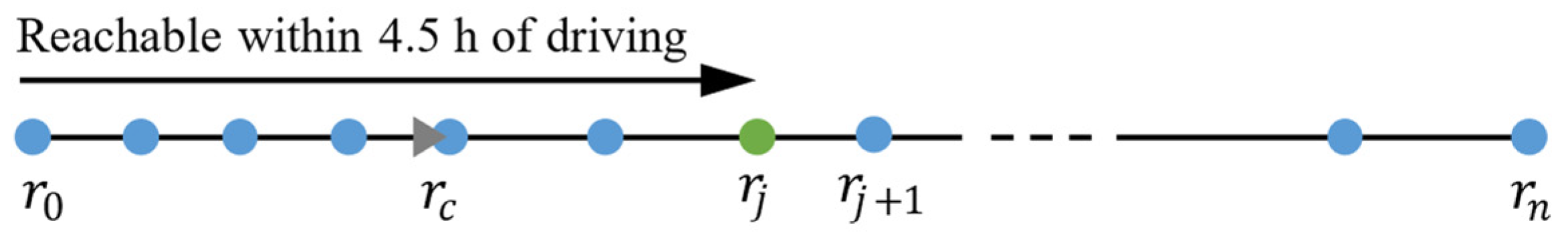
If the next POI can no longer be reached within the allowed driving time of 4.5 h, complete the full rest time, and charge the vehicle at the current POI.

As mentioned in Section 2.2, we use the minimal idle time resulting from charging and resting as an optimization target for BETOS. Both strategies use the same parameterizations in terms of battery limits.

Table 1. Parametrization of charging management strategies, vehicle battery and transport scenario. Both strategies, BETOS and the experienced driver, use the same parametrization.

Parameter	Value/Range
Starting SOC	90%
DOD	100–15%
Cost in DP Optimization	Time
SOC at destination	Min. 15%
Time to Connect/Pay	6 min [33]
Battery Capacity	500 kWh (varied in one case study)
Max. charging rate	3 C
Tour length	650–700 km
Payload	19.3 t

shows all relevant vehicle and charging management parameters, which are kept constant throughout Section 4. All other vehicle model parameters can be found in Appendix A. In Section 2, we proposed a dynamic charging strategy called BETOS. In this section, we briefly introduced the simulation framework for the operation simulation of BET. The following section applies the framework with both charging strategies in different case studies.

4. Application in Different Scenarios

To answer the overarching research question about the potential and influence of optimal charging strategies and appropriate charging infrastructure parameters for currently available BET, we use three different case studies (CS), as specified in

Table 2. Description of different case studies by relevant properties according to charging infrastructure and vehicle. With the three case studies (CS), we aim to answer three research questions about the ecosystem of battery electric trucks. In general, we always compare the proposed dynamic strategy with the decisions of an experienced driver.

Case Study (CS 1–3)	Distance between Two POI	Charging Power at POI	Availability of Charging Station
Idealized static conditions	constant	constant	permanent
Idealized charging network	distribution	distribution	permanent
Real-world charging network	distribution	distribution	probability with waiting time

.

In CS 1, we first show the interaction of vehicle and charging infrastructure for constant conditions in terms of charger density and available charging power. We further show the potential of the optimal strategy compared to driver decisions. CS 1 thus provides a basic understanding of the parameters of the BET ecosystem. In CS 2, we approach the real-world characteristics of the charging infrastructure. We show the impact of density and charging power when assumed in a distributed kind in four different scenarios. The critical simplification, which is still applied in CS 2, is the permanent availability of the POIs. We drop this simplification in CS 3. The POIs are now assigned to an availability probability. For an occupied charging station, a waiting time known in advance must be completed. We show the difference between the NGS strategy and the proposed BETOS algorithm for each CS. For an intuitive metric for this comparison, we show the resulting time loss compared to today’s diesel trucks. The loss of time is attributed to the overall idle time of the BET, subtracting the mandatory rest period of 45 min, a requirement that diesel truck drivers must also adhere to. In case of more than 9 h of driving time, 90 min of required rest time is considered. We first investigate the general dependencies between the truck and infrastructure properties in CS 1.

4.1. Idealized Static Conditions (CS 1)

For the analysis shown below, 100 different transport scenarios (Figure 5) are generated and simulated for a range of battery capacity from 400 to 800 kWh and charging power from 400 to 2000 kW for each combination. The density of the POI was kept constant at 2 POI/100 km. This results in nearly equidistant distances of 50 km between two POIs. Due to the different dynamics of the transport cycles, there is a specific scattering of the resulting time loss for each combination of battery capacity and available charging power. Figure 6a,b below shows the average time loss for each combination for driver and BETOS decisions. It is clearly shown that optimal charging strategies can significantly reduce the expected time loss per trip. Even with high battery capacity and charging power, driver decisions result in an average time loss of 10 to 20 min (Figure 6a). This occurs because, in the case of non-optimal stops, a second stop is required during the second 4.5 h driving period. However, through optimal planning, such a stop can be avoided (Figure 6b) For battery capacities of 550 kWh, a charging power of approximately 1000 kW is sufficient to operate in long-haul applications without time loss compared to diesel trucks in the described scenario. While we present average values over all 100 transport tasks on the left side, Figure 6c displays the observed dispersion of time loss per trip for an installed battery capacity of 500 kWh and an available charging power of 1000 kW. Even if the time loss can be reduced by more than half by optimal charging stops, a higher standard deviation is shown for BETOS than for driver decisions.

Further, it can be observed that a time loss can be avoided for the investigated parameter configuration, even for NGS decisions in a few ideal cases. Under very unfavorable circumstances, even optimal strategies lead to a significant time loss (outliers of BETOS in Figure 6c). This is explained by a second legally required rest stop of 45 min if the second driving interval extends beyond 4.5 h but the total driving time is below 9 h.

To answer the research question (a) from Section 1, the battery size is shown to be the primary driver of time loss. Optimal strategies can significantly reduce the time loss over the entire range analyzed. Under the assumed 50 km distance between two chargers, the combination of 550 kWh battery capacity and 1 MW charging power leads to a time loss of less than 10 min. In the next paragraph, we will analyze more in-depth different infrastructure properties.

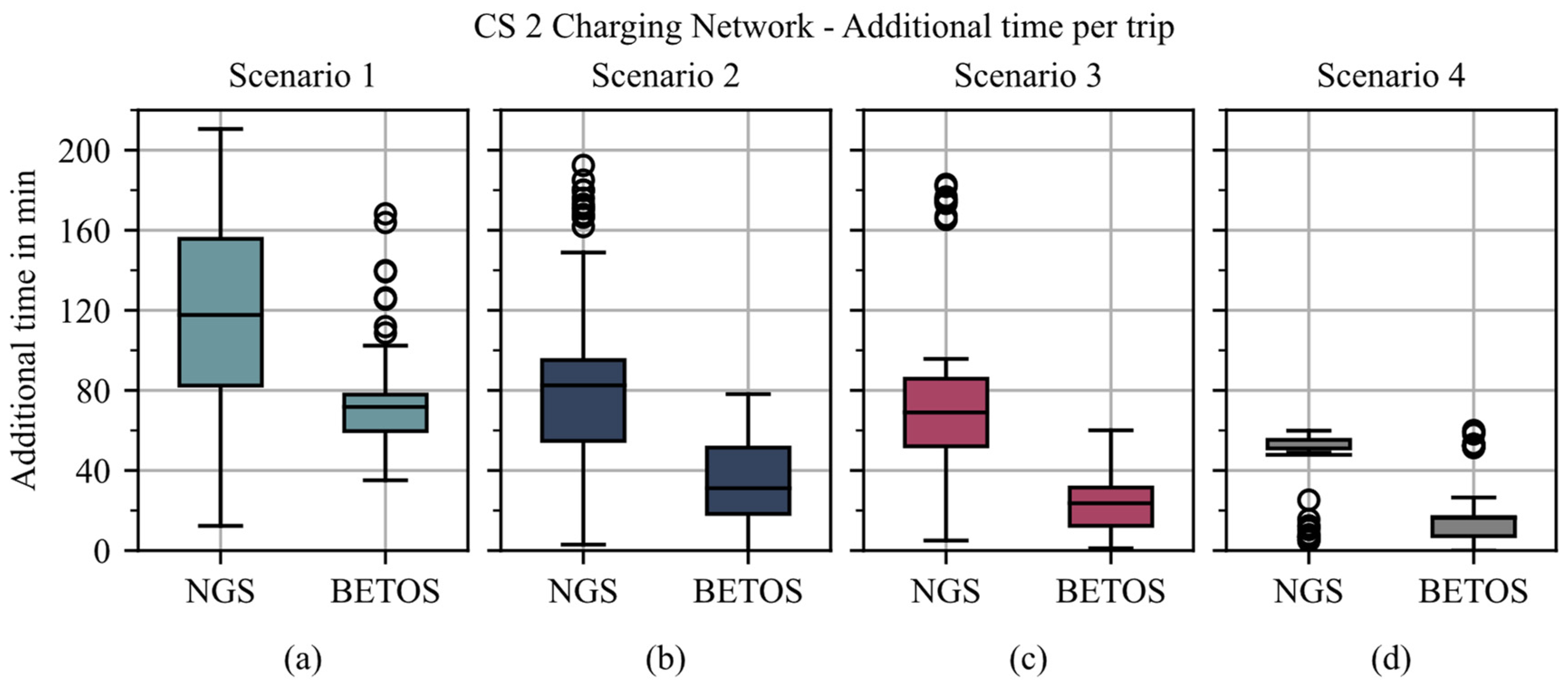
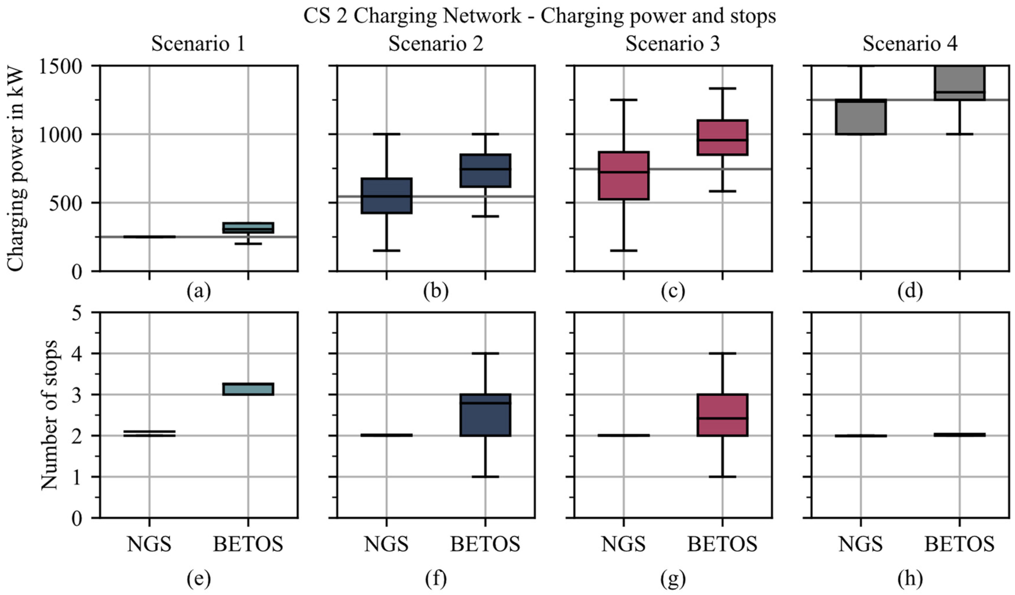
4.2. Idealized Charging Network (CS 2)

In the previous section, we used constant parameters of the charging network. In this section, we now model the infrastructure properties in a probabilistic manner in addition to the transportation profiles, moving closer to the real-world application. Therefore, four different scenarios are compared below.

4.2.1. Charging Network Properties

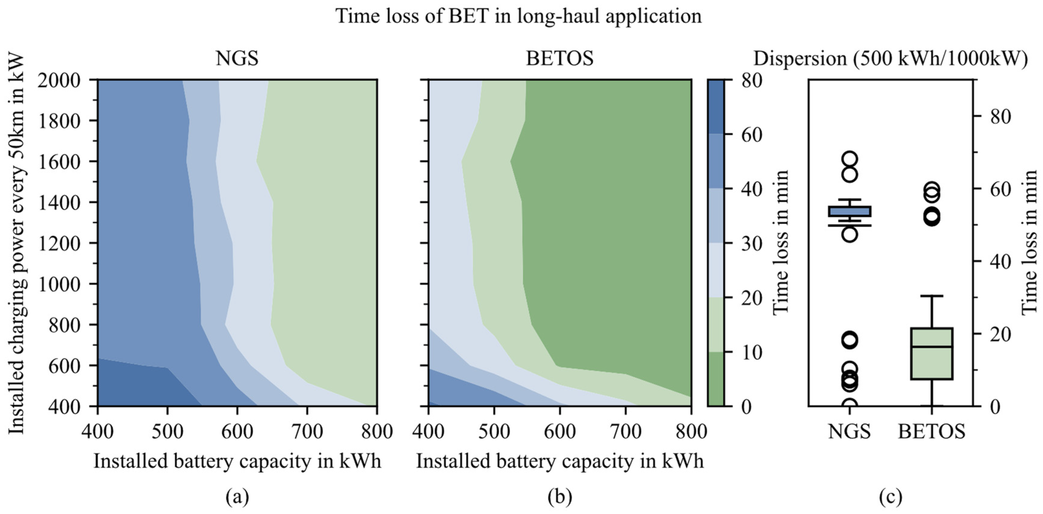
On the vehicle side, we keep the two relevant properties of battery capacity at 500 kWh and a maximum charging rate of 3 C constant. The infrastructure parameters, such as the spatial density, are represented by distributions. Figure 7 compares the four different infrastructure scenarios. Scenario 1 describes an initial charging network with a low density of mostly one charging point per 100 km and limited CCS equipment. Scenario 2 mainly sets a density of two charging points per 100 km. Furthermore, about half of the charging points are also equipped with Megawatt Charging System [39] (MCS) charging points (≥700 kW). Scenarios 1 and 2 are aligned with the newly introduced EU regulations on infrastructure for alternative fuels (AFIR) for the rollout steps until 2025 and 2030 [40]. In Scenario 3, we show the improvement that a very dense and powerful charging network can bring. Scenario 4 further describes an ideal charging network with charging points of at least 1 MW at all rest sites along the highway in Germany [41].

Figure 6. Average time loss of BET in long-haul applications using (a) NGS and (b) BETOS algorithm (b). Per the combination of installed battery capacity and charging power, we simulate 100 long-haul cycles with a trip length between 650 and 700 km and show the average time loss per such trip. Different transport tasks, varying in length and dynamic, result in different energy consumption. We show, on the right, for one combination, the dispersion of expectable time loss across all 100 simulation runs (transport cycles) (c). We used a fixed distance between two POIs of 50 km in alignment with today’s service site density in Germany [42].

Figure 6. Average time loss of BET in long-haul applications using (a) NGS and (b) BETOS algorithm (b). Per the combination of installed battery capacity and charging power, we simulate 100 long-haul cycles with a trip length between 650 and 700 km and show the average time loss per such trip. Different transport tasks, varying in length and dynamic, result in different energy consumption. We show, on the right, for one combination, the dispersion of expectable time loss across all 100 simulation runs (transport cycles) (c). We used a fixed distance between two POIs of 50 km in alignment with today’s service site density in Germany [42].

4.2.2. Results

For the four scenarios presented in Figure 7, we again compare the NGS decisions with those of the presented charging strategy BETOS. Figure 8 shows the resulting time loss compared to a diesel truck using the two strategies. Considering the result for NGS decisions first, there is a continuous improvement in the resulting time loss across all scenarios. No time loss can be expected in exceptional cases from Scenario 2 onwards (Figure 8b). However, the average time loss for Scenario 4 (Figure 8d) is still about 25 min. Using BETOS, the time loss can be reduced by about 50% in all scenarios compared to NGS. The most significant improvement is seen from Scenario 1 (Figure 8a) to Scenario 2 (Figure 8b). A further increase in spatial resolution and performance of the charging infrastructure is only slightly beneficial when using BETOS. However, the maximum time losses can be significantly reduced in Scenario 3 (Figure 8c) and Scenario 4 (Figure 8d). In contrast to CS 1 (Figure 6), the results show a significantly smaller scatter using BETOS than when taking the NGS decisions. This is due to the situationally optimal solutions, which allow for a much better response to locally fluctuating characteristics of the charging infrastructure. Three factors show the time advantage through optimal charging strategies. The targeted use of fast-charging capable POI is essential. Figure 9a–d clearly shows that BETOS selects POIs with higher charging capacities than are available on average across all POIs (gray line), thus explicitly using the POI with high charging power. Two additional factors for the time advantage are the targeted use of the allowed break split and the utilization of the fast-charging SOC range. This is shown in Figure 9e–h. Especially for a low infrastructure resolution, BETOS uses an additional stop to almost halve the time loss (Figure 9a). The denser the charging infrastructure becomes, the more frequently a two-stop strategy is selected. Due to the apparent time advantage over the NGS strategy with almost the same number of stops, BETOS utilizes the fast-charging SOC range.

The research question (b) formulated in Section 1 can thus be answered. Suppose the optimal algorithm BETOS is available to the driver; a spatial resolution of 50 km with charging powers in the 700 to 1000 kW range is necessary to keep the time loss below 30 min on average. Much higher local resolution and charging power are required if drivers follow the rule-based NGS strategy. This is only true if all charging points are always available, as we assumed in CS 1 and CS 2. Therefore, the following section investigates the influence of occupied charging stations.

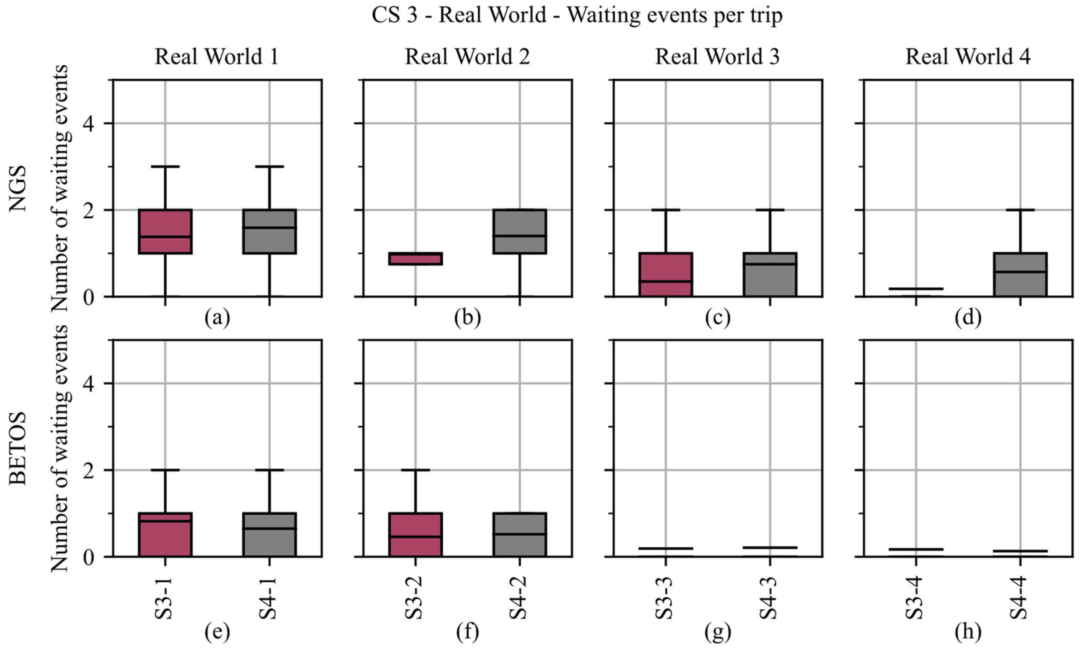
4.3. Real-World Charging Network Conditions (CS 3)

We first assume that probabilities regarding POI availability do not influence drivers’ decisions. It can be assumed that frequently occupied charging points are not selected through experience. However, we do not model such heuristic knowledge in the rule-based strategy used for comparison here. The following subsection shows the integration of availability probabilities in the proposed optimal charging strategy BETOS.

4.3.1. Charging Strategy Adaption for Uncertain Charging Station Availability

Compared to the previous case studies, the POI $r_i$ is now assigned to an availability probability $p_{av,i}$, assuming a constant probability over the whole day. Based on this, the approach shown above cannot be used without further adjustment since the costs can no longer be determined deterministically but depend on whether a POI is free or occupied. Therefore, following the fundamentals of decision theory [44], the expected cumulative cost $E_{i,p,q}$ of a decision is used instead of the deterministic cost $C_{i,p,q}$ (10).

$$E_{i,p,q}=\underset{k,l}{\min }\left(\left(p_{av,i}·\left(C_{d_{i,k,l}}+C_{i+1,p^{\prime },q^{\prime }}\right)\right)+\left(\left(1-p_{av,i}\right)·\left(C_{\prime }^{d_{i,k,l}}+C_{i+1,p^{″},q^{″}}\right)\right)\right)$$

(11)

Thereby applies:

$$s_{i,p,q}\stackrel{d_{i,k,l}}{\to }{s}_{i+1,p^{\prime },q^{\prime }} \mathrm{for} \mathrm{free} \mathrm{POI}$$

(12)

$$s_{i,p,q}\stackrel{d_{i,k,l}}{\to }{s}_{i+1,p^{″},q^{″}} \mathrm{for} \mathrm{occupied} \mathrm{POI}$$

(13)

The cost $C_{\prime }^{d_{i,k,l}}$ is incurred for an occupied POI due to the possible waiting times for the decision $d_{i,k,l}$. The DP approach shown in Section 2.4 is performed based on these expected costs for the analysis of CS 3. If a POI is occupied upon arrival, it can be situationally decided whether the expected cumulative costs are lower when waiting or when driving to the next POI. Consequently, this comparison makes reacting situationally to occupied charging points possible.

For the following application, we assume that the probabilities $p_{av,i}$ are known and do not depend on the daytime, although this is a simplification. Further, we assume a constant waiting time $t_{wait}$ of 15 min to be completed when an occupied POI is selected. Before we present the influence of occupied charging points, we show the scenarios used for this in the next paragraph.

4.3.2. Charging Network Properties

Regarding the POI density and the distribution of the individual POIs’ charging power, we use Scenarios 3 and 4 from CS 2 (Figure 7). We use these two scenarios because, under ideal conditions ($p_{ava}=1$), they show, on average, a slight difference in terms of time loss when using BETOS and consequently would be suitable as a benchmark for the expansion of the charging infrastructure for BET. Based on this, we investigate whether this is true when considering availability probability below 1. As there is currently no charging infrastructure for BET and no data on availability are known, we define four scenarios with different POI availabilities, shown in

Table 3. Additional properties of the real-world charging infrastructure network. Based on Scenarios 3 and 4 (Figure 7), we add the availability probability in four different scenarios while keeping the other properties of Scenario 3 fixed. The last row shows the weighted mean availability probability of each scenario. Due to different frequencies of charging power of positioned POI, there are different weighted mean availabilities of the POI.

Charging Power in kW	Availability Probability of POI
	S 3/4-1	S 3/4-2	S 3/4-3	S 3/4-4
150	1.0	1.0	1.0	1.0
350	0.4	0.6	0.8	1.0
700	0.3	0.5	0.7	0.9
1000	0.2	0.4	0.7	0.8
1500	0.2	0.2	0.6	0.7
Weighted Mean	0.35/ 0.20	0.51/ 0.30	0.74/ 0.65	0.88/ 0.75

. We assume that POIs with high charging power are more popular and have a lower availability probability. Over the scenarios, which we abbreviate as Real-World Scenarios (RWS) 1 to 4 in the following section, the availability of the charging points keeps increasing. For the defined scenarios, we show the impact on time loss for both charging strategies, BETOS and NGS.

4.3.3. Results

Figure 10 illustrates the associated time loss, and Figure 11 displays the count of waiting events encountered, with Scenario 3 depicted in red and Scenario 4 in gray, continuing the color scheme from CS 2.

Suppose the decisions about charging stops are made by NGS (Figure 10a–e), which does not take the information about the probabilities into account in our implementation; there is no increase in the average time loss for RWS 4 (Figure 10d based on Scenario 3 (red) or 4 (grey). Only the maximum values increase for Scenario 4. This is explained by the low number of waiting events, shown in Figure 11d. With the decreasing availability of the POI in RWS 3 to RWS 1, the number of waiting events increases to an average of more than one event per trip. Figure 10a–c shows the resulting and maximum time loss increase compared to ideal or high availabilities. Overall, the effect of occupied charging points on the average time loss when using NGS decisions is relatively small. However, the variance in the results over the 100 simulation runs increases significantly. Even for very low availabilities in RWS 1, the average time loss increases compared to ideal conditions by about the duration of one waiting event of 15 min assumed here.

For BETOS, we have shown the integration of availability probabilities in the previous paragraph. Starting from ideal conditions ($p_{ava,i}=1$) in Figure 10j, the influence of occupied charging points ($p_{ava,i}<1$) is small at high availabilities. In both RWS 3 and 4 (Figure 10h,i), there is only a minimal increase in time loss on average, which is much smaller than the 15 min waiting time in the case of an occupied POI. Figure 11g,h clearly shows that occupied charging points are mostly avoided, and thus, waiting events rarely occur. The increase in the maximum values, which can be observed in Figure 10h,i, can be attributed to charging points with lower power but higher availability (Table 3). For the low availabilities, waiting events cannot be avoided, even when using BETOS, but on average, the number is still below one such event per trip (Figure 11e,f). The experienced waiting events are also shown by an increase in the average time loss in RWS 1 by 15 min (Figure 10f).

Two main insights can be gained from the results of the third case study, CS 3, which simultaneously answers the posed research question from Table 3.

First, the BETOS algorithm reacts more sensitively to realistic infrastructure properties due to the situationally optimal decisions. For medium and high availabilities, the waiting times assumed here can be compensated well (Figure 10h–j) or are bypassed by choosing POIs that tend to be more available (Figure 11g,h).

Second, independent of the decision making (BETOS or NGS), the availability of $p_{ava,mean}>0.75$ (RWS 4) is desirable. For POIs available, hardly any disadvantage compared to the ideal conditions could be observed for the waiting time of 15 min assumed here. This answers research question (c) stated in Section 1.

In the previous paragraphs, we demonstrated the performance of the dynamic charging strategy in three case studies. For today’s battery capacities of BET, we have also analyzed various infrastructure scenarios and can thus derive recommendations for action, as summarized in Section 6. However, the BETOS strategy presented requires a high level of information about vehicle and infrastructure parameters. We refer to this in the following sensitivity analysis.

5. Sensitivity Analysis

In Section 2.3, we already pointed out the necessity of predicting properties such as energy consumption or travel times when describing the optimization problem. In addition to these predictions on the vehicle side, in Section 4.3, we assumed information about the availability and waiting times of the POI and, thus, the prediction of these infrastructure parameters. Therefore, we highlight the importance of this information provided by charge point operators (CPO) in the future by investigating the influence on time loss if such information is inaccessible. In addition, Hecht et al. [26] show a high dependence on SOC at the start of driving on time loss in their work. We examine whether such dependence is also observable for BET in Section 5.3.

5.1. Influence of Information Loss

Section 4.3 has shown that charging point availabilities for medium and high availabilities (RWS 3/4) can be well compensated by BETOS. We want to explicitly shed light on this again by removing the information about POI availabilities and waiting time from the presented strategy and comparing this to the results with full knowledge of these properties. We show this analysis based on Scenario 4 from CS 2. However, the availabilities differ in the three scenarios considered to gain insights into the importance of providing information about availability and waiting time (

Table 4. Scenario description for the analysis of the impact in case of no information about the availability and expected waiting time of POI. Along the route, two types of chargers with different power and availability can occur. The availability of the 1500 kW charger decreases from S 4–5 to S 4–7, while the 1000 kW chargers are always available.

Charging Power in kW	Availability Probability of POI
	S4–5	S4–6	S4–7
1000	1.0	1.0	1.0
1500	0.8	0.5	0.2

).

Figure 12 shows the influence of information loss on time loss when using BETOS in the usual way. For all scenarios considered, there is a significant increase in the maximum time loss when information is lost. However, even poorly available charging points can be bypassed using BETOS if the information is available. The average time loss and the maximum values increase only minimally compared to the ideal conditions (Figure 12c). Only for generally high availabilities in S 4–5 is the information loss manageable in terms of mean time loss.

In summary, providing such information about the POIs is highly relevant. The BET charging infrastructure should be expanded by digital backend systems to provide such information. If this information is available, this investigation shows that the integration and use of it in BETOS provide plausible results.

5.2. Influence of Prediction Errors

In addition to the information about POI properties, the vehicle parameters, energy consumption, and travel time between POIs must be predicted or known for both charging strategies. In addition, BETOS uses the charging maps shown in Figure 5 due to its online capability and fast computation. These will also be subject to errors, as the vehicle battery and the charging station may reduce their charging power for various reasons. However, we do not investigate such errors here because it is evident that they lead to a longer charging time than expected. Therefore, the focus will be on the two properties of energy consumption and travel time. For each distance step of the transport scenario (Figure 6), an error in time and the required energy for this distance step are applied. The magnitude of the error is assumed to be an interval and is determined stochastically according to a uniform distribution (

Table 5. Applied prediction errors for the following sensitivity analysis. We apply up to 15% error in energy and time prediction, meaning the decisions are based on this forecast.

Property	Error Interval	Description
Energy consumption	[−15, 0]%	Prediction of less energy consumption than needed.
Driving time	[−15, 0]%	Prediction of less time than needed.

).

Figure 13 shows, in analogy to (Section 4.2), the influence of these prediction errors on the resulting time loss for the scenarios considered in CS 2. The prediction errors assumed here are negligible in their influence on the time loss. The structure of BETOS can explain this. The situational optimal solution is found at each upcoming POI based on the current system state. Even with few POIs in Scenario 1, the optimal solution is often updated enough to compensate for prediction errors. For the errors in the time prediction, it should be noted that we examined always available charging points analogous to CS 2. In the current implementation of BETOS, CS 3 is also assumed to have constant availabilities throughout the day. For POI availabilities that are daytime dependent, errors in driving time can be much more severe.

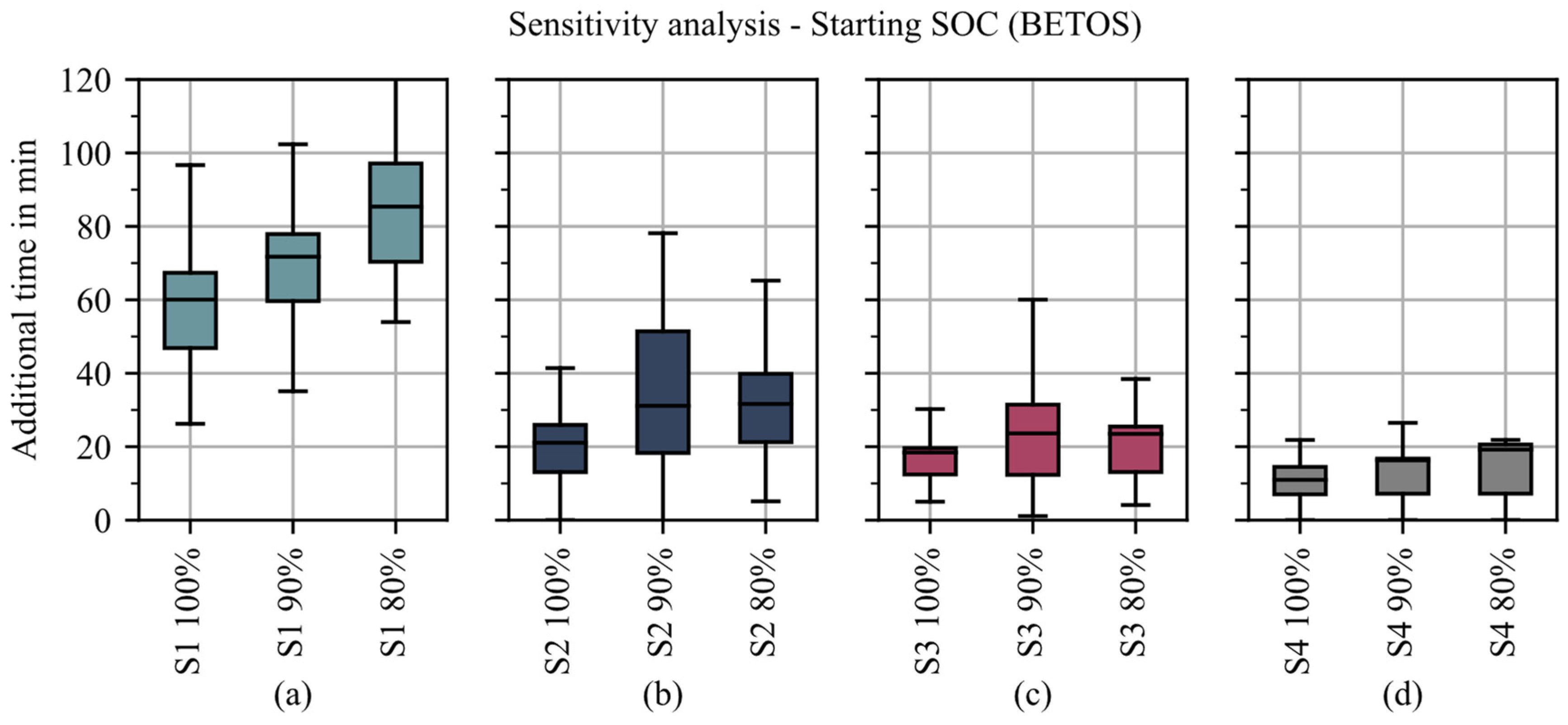
5.3. Influence of Starting Conditions

Finally, we want to investigate the influence of the starting conditions on the time loss. For this purpose, we consider the scenarios from CS 2. Figure 14 shows that the starting SOC’s influence decreases as the charging infrastructure’s performance increases, and for a near-ideal infrastructure in CS 4, it only shows up marginally. In addition, the step from 90% to 100% starting SOC brings significant improvements, but from Scenario 2 onwards, the step from 90% to 80% seems hardly beneficial. In summary, the private charging infrastructure should be sized for poorly developed public charging infrastructure so the BET can start with a fully charged battery. For a well-developed public charging infrastructure, a start with 80% SOC is only slightly disadvantageous and offers the downsizing of cost-intensive private charging infrastructure.

The sensitivity analysis has shown that the proposed algorithm can handle real charging infrastructure properties and make plausible decisions even when charging points are occupied (Section 5.1). The performance is less dependent on prediction errors on the scale studied here concerning vehicle characteristics (Section 5.2). The starting condition of the truck battery has a high impact in the case of low-developed public charging infrastructure. However, it takes a subordinate role in a widely available and powerful infrastructure (Section 5.3).

6. Discussion

We divide the discussion into three subsections. Besides the presented algorithm as such, the results of the simulation studies will be discussed in detail. As a third subsection, we derive recommendations for the efficient holistic rollout of BET in long-haul applications.

6.1. Algorithm

In this work, we presented an online charging strategy for BET that makes situationally optimal decisions regarding charging time and rest time. Compared to decisions a driver would make, BETOS halved the time loss due to charging events compared to today’s diesel trucks for all infrastructure scenarios studied (Section 4). We further showed that BETOS makes safe and plausible decisions even in the case of occupied charging sites.

In terms of computation time and thus ensuring online capability, decision making takes an average of 0.849 s for simulation on a MacBook Pro M1 when availability probabilities are included. In comparison, the rule-based strategy is clearly faster, with 0.093 s. These values apply to the discretization assumed here for the decision space of 1% steps in the SOC and 1 min steps in the charging time (Section 2.4).

Future work could investigate how optimized discretization reduces the computation while ensuring adequate accuracy. One option is dynamic or non-equidistant discretization, depending on the available charging power at a POI. Essential for the low computation time is the use of the charging maps shown in Figure 4, which provide the end SOC as a lookup table for each starting SOC and hit charging time. Since we do not use a thermoelectric model of the battery system, we neglect the dependence on temperature and the influence of the internal resistance increase over the lifetime. In the future, the charging maps can be extended to include the dimensions of temperature and state of health. However, this requires integrating an aging model. In addition to the algorithm, we would like to refer to the results of the performed case studies next.

6.2. Simulation Studies and Results

With the help of the presented charging strategy and the framework for the simulation of transport scenarios, we have investigated different charging infrastructure scenarios and evaluated them concerning the resulting time loss. To minimize statistical effects arising from the probabilistic properties of the infrastructure model and the transport cycles, we simulated 100 cycles per investigation. However, the whiskers of the shown box plots do not always exhibit consistent results (e.g., Figure 10), which can be attributed to such effects. Instead, the lower and upper quartiles are consistent over these scenarios.

The decisive properties of the charging infrastructure are the density, the charging power, and the availability of the charging stations. However, more is needed for a complete design of the charging infrastructure since a central parameter, the number of charging points per POI, cannot be derived from this. With the help of the minimum required availability (Section 4.3), this missing parameter can be determined in future work with the support of traffic data that provide information about the number of trucks on concrete routes. Moreover, this work uses time as a cost function in the presented charging strategy. The integration of a comprehensive cost function that considers time in the form of opportunity costs, battery degradation in the form of replacement costs, and charging costs will be sought in future work.

Besides this, it should also be mentioned that we have assumed the charging behavior shown in Figure 4 and allowed for a peak charging rate of up to 3 C. Based on this, the assumed battery capacity of 500 kWh already shows itself to be suitable for use in long-distance transport. Future work could show whether higher battery capacities can provide noticeable benefits, as the charging power and, consequently, the stress on the battery can be reduced. The results shown, the sensitivity analysis carried out, and the aspects discussed are summarized below in recommendations for the efficient rollout of BET in long-haul transport.

6.3. Recommendations for Efficient Operation of Battery Electric Trucks in Long-Haul Application

The following recommendations apply to the assumptions and simplifications discussed above. On the vehicle side, battery capacities of around 500 kWh and charging rates of 3 C are shown to be suitable for use in long-haul transport with an appropriate charging infrastructure. For spatial distribution of 50 km on average and a charging power between 700 kW and 1.5 MW, the time losses can be kept below 30 min on average with availabilities of the POI above 75%. While the resolution corresponds to the objective of the AFIR [40], the charging capacity of 350 kW stipulated in it is too low and, therefore, should be increased to 1 MW.

If such time losses are not acceptable from the forwarder’s point of view, only an increase in battery capacity can provide a remedy; the densification of the charging network yields only improvements in case of availability close to 100% here. The results have shown that dynamic charging strategies provide significant advantages and should be used in future BET. Digital backend systems of the charging infrastructure are imperative to predict the availabilities of the POI. Regarding the currently discussed reservation systems for BET charging sites, it is shown that availabilities of about 75% on average do not cause any noticeable deterioration compared to ideal, consistently reserved charging points. For higher battery capacities, however, it can be assumed that the time loss can be eliminated plannable using reservation systems. On the other hand, increased investment for the expansion of public charging infrastructure must be expected since a higher number of charging points per POI must be installed to cover the charging demand of BET despite reserved charging points. This needs to be investigated in future work. We close this work with a brief conclusion.

7. Summary and Outlook

Battery electric trucks offer the leading technology for decarbonizing road freight due to their high well-to-wheel efficiency. Due to the limited range caused by installation space and payload, the efficient use of BET in long-distance transport requires an optimal charging strategy. In the scope of this work, we demonstrated a robust online algorithm for the optimal integration of charging stops. We used this to analyze different charging infrastructure scenarios and outline recommendations for the efficient rollout of BET in long-haul applications. Our recommendations can be summarized by the following properties of the BET ecosystem: A BET with a battery capacity of 500 kWh, a density of 50 km, and an available charging power of 1 MW with an availability of 75% on average is suitable. Optimal charging strategies can significantly reduce the time loss compared to today’s diesel trucks and, therefore, ensure the efficient rollout of BET. A detailed sensitivity analysis showed that the presented algorithm provides plausible results. In future work, charging costs and battery degradation could be integrated into the charging strategy in addition to time. Furthermore, the daytime-dependent availability of POIs could be taken into account. Besides this, we will extend the framework shown through a real charging network in Germany and Europe in order to be able to give a complete proposal for a suitable charging network for BET in long-distance traffic with the help of freight transport data [45] and thus make a further contribution to the decarbonization of the transport sector.

References

1. European Commission. Directorate General for Mobility and Transport. EU Transport in Figures: Statistical Pocketbook 2022. LU: Publications Office, 2022. Available online: https://data.europa.eu/doi/10.2832/216553 (accessed on 2 June 2023).
2. European Commission. Directorate General for Climate Action. Going Climate-Neutral by 2050: A Strategic Long Term Vision for a Prosperous, Modern, Competitive and Climate Neutral EU Economy. LU: Publications Office, 2019. Available online: https://data.europa.eu/doi/10.2834/02074 (accessed on 2 June 2023).
3. e-Truck Studie 2023|Tankkarten und Services für Ihr Flottenmanagement|Tankkarte & Ladekarte—Flottenmanagement Services|Aral, Aral Card. Available online: https://www.aral.de/de/global/fleet_solutions/aral-flottenloesungen/e-Truck-Studie-2023.html (accessed on 2 June 2023).
4. European Union. Directive (EU) 2022/2464 of the European Parliament and of the Council of 14 December 2022 Amending Regulation (EU) No 537/2014, Directive 2004/109/EC, Directive 2006/427EC and Directive 2013/34/EU, as Regards Corporate Sustainability Reporting; European Union: Brussels, Belgium, 2022. [Google Scholar]
5. Huang, W.-D.; Zhang, Y.-H.P. Energy Efficiency Analysis: Biomass-to-Wheel Efficiency Related with Biofuels Production, Fuel Distribution, and Powertrain Systems. PLoS ONE 2011, 6, e22113. [Google Scholar] [CrossRef] [PubMed]
6. Cunanan, C.; Tran, M.K.; Lee, Y.; Kwok, S.; Leung, V.; Fowler, M. A Review of Heavy-Duty Vehicle Powertrain Technologies: Diesel Engine Vehicles, Battery Electric Vehicles, and Hydrogen Fuel Cell Electric Vehicles. Clean Technol. 2021, 3, 474–489. [Google Scholar] [CrossRef]
7. Volvo FH Electric. Available online: https://www.volvotrucks.de/de-de/trucks/trucks/volvo-fh/volvo-fh-electric.html (accessed on 7 December 2023).
8. Showroom|Mercedes-Benz Trucks. Available online: https://eactros600.mercedes-benz-trucks.com/de/de/eactros-600/showroom.html (accessed on 7 December 2023).
9. MAN Truck & Bus SE, Elektro-Lkw|MAN DE. Available online: https://www.man.eu/de/de/lkw/elektro-lkw/uebersicht.html (accessed on 7 December 2023).
10. Lahmann, S. Aktivitäten zur Nutzfahrzeug Ladeinfrastruktur, Presented at the BMDV Fachkonferenz Klimafreundliche Nutzfahrzeuge, November 2022. Available online: https://www.now-gmbh.de/wp-content/uploads/2022/11/NFZ22_Aktivitaeten-zur-Nutzfahrzeug-Ladeinfrastruktur_Lahmann.pdf (accessed on 7 December 2023).
11. Charging the Future of Road Transport, Milence. Available online: https://milence.com/ (accessed on 6 February 2024).
12. Bp Pulse Builds Europe’s First Public Charging Corridor for Electric Trucks Along Major Logistics Route|News and Insights|Home, bp Global. Available online: https://www.bp.com/en/global/corporate/news-and-insights/press-releases/bp-pulse-build-europes-first-public-charging-corridor-for-electric-trucks-along-major-logistics-route.html (accessed on 6 February 2024).
13. Plötz, P. Hydrogen technology is unlikely to play a major role in sustainable road transport. Nat. Electron. 2022, 5, 8–10. [Google Scholar] [CrossRef]
14. Nykvist, B.; Olsson, O. The feasibility of heavy battery electric trucks. Joule 2021, 5, 901–913. [Google Scholar] [CrossRef]
15. Link, S.; Plötz, P. Technical Feasibility of Heavy-Duty Battery-Electric Trucks for Urban and Regional Delivery in Germany—A Real-World Case Study. World Electr. Veh. J. 2022, 13, 161. [Google Scholar] [CrossRef]
16. Wolff, S.; Seidenfus, M.; Brönner, M.; Lienkamp, M. Multi-disciplinary design optimization of life cycle eco-efficiency for heavy-duty vehicles using a genetic algorithm. J. Clean. Prod. 2021, 318, 128505. [Google Scholar] [CrossRef]
17. Mareev, I.; Becker, J.; Sauer, D.U. Battery Dimensioning and Life Cycle Costs Analysis for a Heavy-Duty Truck Considering the Requirements of Long-Haul Transportation. Energies 2018, 11, 55. [Google Scholar] [CrossRef]
18. Teichert, O.; Link, S.; Schneider, J.; Wolff, S.; Lienkamp, M. Techno-economic cell selection for battery-electric long-haul trucks. eTransportation 2023, 16, 100225. [Google Scholar] [CrossRef]
19. Karlsson, J.; Grauers, A. Case Study of Cost-Effective Electrification of Long-Distance Line-Haul Trucks. Energies 2023, 16, 2793. [Google Scholar] [CrossRef]
20. Schneider, J.; Teichert, O.; Zähringer, M.; Balke, G.; Lienkamp, M. The novel Megawatt Charging System standard: Impact on battery size and cell requirements for battery-electric long-haul trucks. eTransportation 2023, 17, 100253. [Google Scholar] [CrossRef]
21. Depcik, C.; Gaire, A.; Gray, J.; Hall, Z.; Maharjan, A.; Pinto, D.; Prinsloo, A. Electrifying Long-Haul Freight—Part II: Assessment of the Battery Capacity. SAE Int. J. Commer. Veh. 2019, 12, 87–102. [Google Scholar] [CrossRef]
22. Mauler, L.; Dahrendorf, L.; Duffner, F.; Winter, M.; Leker, J. Cost-effective technology choice in a decarbonized and diversified long-haul truck transportation sector: A U.S. case study. J. Energy Storage 2022, 46, 103891. [Google Scholar] [CrossRef]
23. EU-Parlament, Verordnung (EG) Nr. 561/2006 des Europäischen Parlaments und des Rates vom 15. März 2006 zur Harmonisierung bestimmter Sozialvorschriften im Straßenverkehr und zur Änderung der Verordnungen (EWG) Nr. 3821/85 und (EG) Nr. 2135/98 des Rates sowie zur Aufhebung der Verordnung (EWG) Nr. 3820/85 des Rates. Available online: https://www.balm.bund.de/DE/Themen/RechtsentwicklungRechtsvorschriften/Rechtsvorschriften/Fahrpersonalrecht/fahrpersonalrecht_node.html (accessed on 19 April 2023).
24. Speth, D.; Plötz, P.; Funke, S.; Vallarella, E. Public fast charging infrastructure for battery electric trucks—A model-based network for Germany. Environ. Res. Infrastruct. Sustain. 2022, 2, 025004. [Google Scholar] [CrossRef]
25. Auer, J.; Link, S.; Plötz, P. Public Charging Locations for Battery Electric Trucks: A GIS-Based Statistical Analysis Using Real-world Truck Stop Data for Germany. 2023. Available online: https://publica.fraunhofer.de/handle/publica/439538 (accessed on 19 April 2023).
26. Hecht, C.; Victor, K.; Zurmühlen, S.; Sauer, D.U. Electric vehicle route planning using real-world charging infrastructure in Germany. eTransportation 2021, 10, 100143. [Google Scholar] [CrossRef]
27. Erdelić, T.; Carić, T. A Survey on the Electric Vehicle Routing Problem: Variants and Solution Approaches. J. Adv. Transp. 2019, 2019, e5075671. [Google Scholar] [CrossRef]
28. Zähringer, M.; Wolff, S.; Schneider, J.; Balke, G.; Lienkamp, M. Time vs. Capacity—The Potential of Optimal Charging Stop Strategies for Battery Electric Trucks. Energies 2022, 15, 7137. [Google Scholar] [CrossRef]
29. Sweda, T.M.; Dolinskaya, I.S.; Klabjan, D. Adaptive Routing and Recharging Policies for Electric Vehicles. Transp. Sci. 2017, 51, 1326–1348. [Google Scholar] [CrossRef]
30. Guillet, M.; Hiermann, G.; Kröller, A.; Schiffer, M. Electric Vehicle Charging Station Search in Stochastic Environments. Transp. Sci. 2022, 56, 483–500. [Google Scholar] [CrossRef]
31. Bai, T.; Li, Y.; Johansson, K.H.; Mårtensson, J. Rollout-Based Charging Strategy for Electric Trucks with Hours-of-Service Regulations. arXiv 2023, arXiv:2303.08895. [Google Scholar] [CrossRef]
32. Balke, G.; Adenaw, L. Heavy commercial vehicles’ mobility: Dataset of trucks’ anonymized recorded driving and operation (DT-CARGO). Data Brief 2023, 48, 109246. [Google Scholar] [CrossRef]
33. Cussigh, M.; Hamacher, T. Optimal Charging and Driving Strategies for Battery Electric Vehicles on Long Distance Trips: A Dynamic Programming Approach. In Proceedings of the 2019 IEEE Intelligent Vehicles Symposium (IV), Paris, France, 9–12 June 2019; IEEE Press: New York, NY, USA, 2019; pp. 2093–2098. [Google Scholar] [CrossRef]
34. Huber, G.; Bogenberger, K. Long-Trip Optimization of Charging Strategies for Battery Electric Vehicles. Transp. Res. Rec. 2015, 2497, 45–53. [Google Scholar] [CrossRef]
35. Wassiliadis, N.; Steinsträter, M.; Schreiber, M.; Rosner, P.; Nicoletti, L.; Schmid, F.; Ank, M.; Teichert, O.; Wildfeuer, L.; Schneider, J.; et al. Quantifying the state of the art of electric powertrains in battery electric vehicles: Range, efficiency, and lifetime from component to system level of the Volkswagen ID.3. eTransportation 2022, 12, 100167. [Google Scholar] [CrossRef]
36. Fontaras, G.; Rexeis, M.; Dilara, P.; Hausberger, S.; Anagnostopoulos, K. The Development of a Simulation Tool for Monitoring Heavy-Duty Vehicle CO2 Emissions and Fuel Consumption in Europe; SAE Technical Paper 2013-24-0150; SAE International: Warrendale, PA, USA, 2013. [Google Scholar] [CrossRef]
37. European Union. Verordnung (EU) 2018/858 Des Europäischen Parlamentes und Rates vom 30. Mai 2018 über die Genehmigung und die Marktüberwachung von Kraftfahrzeugen und Kraftfahrzeuganhängern sowie Systemen, Bauteilen und selbstständigen technischen Einheiten für diese Fahrzeuge, zur Änderung der Verordnung (EG) Nr. 715/2007 und (EG) 595/2009 und zur Aufhebung der Richtlinie 2007/46/EG.; European Union: Brussels, Belgium, 2018. [Google Scholar]
38. Austin, T.; DiGenova, F.; Carlson, T.; Joy, R.; Gianolini, K.A. Characterization of Driving Patterns and Emissions from Light-Duty Vehicles in California. Final Report. November 1993. Available online: https://www.semanticscholar.org/paper/Characterization-of-driving-patterns-and-emissions-Austin-DiGenova/165fabafa081938fe77d9c432b4944ea867d16c0 (accessed on 26 May 2023).
39. CharIN Whitepaper—Megawatt Charging System (MCS). 24 November 2022. Available online: https://www.charin.global/technology/mcs/ (accessed on 2 February 2024).
40. European Parliament. Regulation (EU) 2023/1804 of the European Parliament and the Council of 13 September 2023 on the Deployment of Alternative Fuels Infrastructure, and Repealing Directive 2014/94/EU.; European Parliament: Strasbourg, France, 2023. [Google Scholar]
41. Bundesregierung Deutschland. Masterplan Ladeinfrastruktur II der Bundesregierung; Bundesregierung Deutschland: Berlin, Germany, 2022. [Google Scholar]
42. Bundesministerium für Digitales und Verkehr. Nebenbetriebe/Rastanlagen; Bundesministerium für Digitales und Verkehr: Berlin, Germany, 2021. [Google Scholar]
43. European Electric Vehicle Charging Infrastructure Masterplan. ACEA—European Automobile Manufacturers’ Association. Available online: https://www.acea.auto/publication/european-electric-vehicle-charging-infrastructure-masterplan/ (accessed on 25 May 2023).
44. Kahneman, D.; Tversky, A. Prospect Theory: An Analysis of Decision under Risk. Econometrica 1979, 47, 263. [Google Scholar] [CrossRef]
45. BMDV—Verkehrsverflechtungsprognose 2030. Available online: https://bmdv.bund.de/Shared-Docs/DE/Arti-kel/G/verkehrsverflechtungsprognose-2030.html (accessed on 16 June 2023).
46. Earl, T.; Mathieu, L.; Cornelis, S.; Kenny, S.; Ambel, C.C.; Nix, J.C. Analysis of Long Haul Battery Electric Trucks in EU Marketplace and Technology, Economic, Environmental, and Policy Perspectives. Available online: https://www.semanticscholar.org/paper/Analysis-of-long-haul-battery-electric-trucks-in-EU-EarlMathieu/21e0357feec21a0f6a4023b739e78855a81-40bfe (accessed on 19 April 2023).
47. Wolff, S.; Kalt, S.; Bstieler, M.; Lienkamp, M. Influence of Powertrain Topology and Electric Machine Design on Efficiency of Battery Electric Trcuks—A Simulative Case-Study. Energies 2021, 14, 328. [Google Scholar] [CrossRef]
48. MAN Truck & Bus SE, Internal Discussion on Powertrain Parameters. 2022.
49. Verbruggen, F.J.R.; Rangarajan, V.; Hofman, T. Powertrain design optimization for a battery electric heavy-duty truck: 2019 American Control Conference (ACC 2019). In Proceedings of the 2019 American Control Conference, ACC 2019, Philadelphia, PA, USA, 10–12 July 2019; pp. 1488–1493. [Google Scholar] [CrossRef]
50. Fries, M.; Wolff, S.; Horlbeck, L.; Kerler, M.; Lienkamp, M.; Burke, A.; Fulton, L. Optimization of hybrid electric drive system components in long-haul vehicles for the evaluation of customer requirements. In Proceedings of the 2017 IEEE 12th International Conference on Power Electronics and Drive Systems (PEDS), Honolulu, HI, USA, 12–15 December 2017; pp. 1–141. [Google Scholar] [CrossRef]
51. Naunheimer, H.; Bertsche, B.; Ryborz, J.; Novak, W.; Fietkau, P. Fahrzeuggetriebe: Grundlagen, Auswahl, Auslegung und Konstruktion; Springer: Berlin/Heidelberg, Germany, 2019. [Google Scholar] [CrossRef]
52. König, A.; Nicoletti, L.; Schröder, D.; Wolff, S.; Waclaw, A.; Lienkamp, M. An Overview of Parameter and Cost for Battery Electric Vehicles. World Electr. Veh. J. 2021, 12, 21. [Google Scholar] [CrossRef]
Figure 1. Visualization of C1 with the route from POI r 0 to r n and the current position along the route r c . The critical POI r j is the furthest POI which can be reached within the total driving time of 4.5 h from the beginning of the trip. When leaving POI r j , the total rest time (45 min) must be completed. In this case, a rest of 45 min is taken, e.g., at POI r c , and the destination is not reachable within 4.5 h, and a new critical POI has to be considered.
Energies 17 00973 g001
Figure 2. Visualization of implemented DP approach for solving the defined optimization problem. To find the best decision out of the decision space at the arrival state in the state space at POI s c , p , q , a backpropagation from the destination r n to the current POI r c is performed. Based on the defined initial cost matrix C n at the destination, the best decision for every arrival state at every POI is the one that results in the minimum cumulated cost. The initial cost matrix specifies the desirable arrival SOC at the destination in terms of costs.
Energies 17 00973 g002
Figure 3. Pseudo algorithm of DP approach for dynamic charging strategy for battery electric trucks in long-haul application. The shown algorithm is performed at every upcoming POI r c for finding the situational optimal decision d c , k , l * . The HoS regulations are considered by calculating the landing system state when choosing a decision and by adjusting the cost matrix with very high costs for not-allowed systems states at the POI after the critical one.
Energies 17 00973 g003
Figure 4. (a) Implemented charging profiles depending on the SOC for different maximum charging rates. For the generation of those, we use a CP-CV charging strategy applied to an equivalent circuit model parametrized with the cell data from [35]; (b) exemplary charging map for 500 kWh of battery capacity, 3 C of peak charging rate and 1500 kW of available charging power. The map is to read: Starting from 50% SOC (x-axis) spending 10 min of charging (y-axis), the resulting SOC would be about 70%. These maps are used in the DP optimization as lookup tables and incorporate the non-linear charging behavior from (a). For example, starting from 20% of SOC and spending 10 min for charging leads to 60%, whereas spending 20 min leads to slightly over 80% of SOC.
Energies 17 00973 g004
Figure 5. Exemplary transport driving cycle as chained microtrips with positioned charging infrastructure as POI. Initial POIs (green) are set at the end of a microtrip. For the additional POIs (blue), the distance between two POIs is modeled as a probability function.
Energies 17 00973 g005
Figure 7. Parametrization of the infrastructure model for four different scenarios. The main parameters are the spatial distribution (a) and the installed charging power (b). Scenario 1 describes very sparse public infrastructure with CCS charging stations and an average charging power of 250 kW. We expect such a scenario to be realized in the next years. Scenario 2, with an average power of 545 kW, is close to Germany’s initially planned charging network according to Masterplan Charging Infrastructure [42] and the European approach from ACEA [43] as well as the AFIR [40]. It is equipped with Combined Charging System (CCS) and MCS charging stations. Scenario 3 (average power 745 kW) assumes a tight and powerful charging network. In Scenario 4, we show an idealized charging network with high density and average power of 1250 kW.
Energies 17 00973 g007
Figure 8. Comparison of resulting time loss in different scenarios (ad) when using BET with 500 kWh installed battery capacity in long-haul application with a daily trip length of 650–700 km. The black line within the boxplots shows the mean values and the black circles mark the outliers. Using BETOS instead of NGS leads to significantly less time loss. Additionally, it is shown that the deviation of the time loss can be significantly reduced by using an optimal charging strategy.
Energies 17 00973 g008
Figure 9. Average chosen charging power (ad) and taken stops (eh) according to driver and BETOS decisions in Scenarios 1 to 4 considered. The grey lines show the average available charging power of all POIs in the different scenarios in alignment with Figure 5. It is clearly shown that BETOS chooses the more powerful charging stations as one reason for the advantage according to time loss compared to rule-based NGS decisions. Furthermore, it is shown that BETOS uses more stops, meaning the fast-chargeable SOC range is selected and overcompensates the additional time for connecting and leaving the highway.
Energies 17 00973 g009
Figure 10. Comparison of resulting time loss using driver and BETOS algorithm decisions operating on RWS 1 to 4 based on Scenario 3 and 4 from CS 2. The top row (ae) shows the influence using NGS decisions, and the bottom row (fj) in the case of BETOS decisions. If a POI is occupied, a waiting time of 15 min is considered.
Energies 17 00973 g010
Figure 11. Comparison of the number of waiting events due to occupied POI using NGS (ad) and BETOS (e,f) decisions. The proposed charging strategy BETOS leads to significantly fewer waiting events over all scenarios. For RWS 3 (g) and 4 (h), the waiting events can be prevented in most cases.
Energies 17 00973 g011
Figure 12. Influence of lost information (NI) about availability probabilities of the POI on the time loss in the three considered scenarios (ac) (Table 4). It is shown that the BETOS algorithm reliably bypasses poorly available charging points. Of course, with increasing inhomogeneity, access to such information becomes more critical.
Energies 17 00973 g012
Figure 13. Impact of time and SOC prediction errors for all different scenarios (ad) considered in CS 2. Due to the dynamic strategy BETOS, meaning finding the situational best decision at every POI, the influence of SOC and time prediction errors up to 15% is neglectable. This holds for all scenarios considered.
Energies 17 00973 g013
Figure 14. Impact of SOC at trip start on the resulting time loss for all scenarios considered in CS 2 (ad). For worse infrastructure (a), the starting SOC has a significant influence on the time loss. This does not hold for even better infrastructure properties (c,d).
Energies 17 00973 g014