Current Compensation Method in a Distribution System Based on a Four-Leg Inverter under Unbalanced Load Conditions Using an Artificial Neural Network

Abstract

This study proposes an unbalanced current compensation method based on a four-leg inverter using an artificial neural network (ANN) under unbalanced load conditions. Distribution systems exhibit rapid load variations, and conventional filter-based control methods suffer from the drawback of requiring an extended time period to reach a steady state. To address this problem, an ANN is applied to calculate the unbalanced current reference and enhance dynamic performance. Additionally, because of the periodic incorrect output inherent in the ANN, applying it to a proportional–integral controller would result in an error being directly reflected in the current reference. In the aforementioned problem, an ANN is applied to the dq0 coordinate system current controller to compensate for the periodic incorrect output in the current reference calculation. The proposed ANN-based unbalanced current compensation method is validated through PSIM simulations and experiments.

1. Introduction

In recent years, power systems have become increasingly complex owing to continuous advancements. In particular, with the rising demand for power, the integration of renewable energy sources, and the introduction of electric vehicles and distributed power generation systems, power networks are now operating in dynamic and diverse environments. These conditions can deteriorate power quality, significantly affecting the stability and performance of power systems. Factors that contribute to the degradation of power system quality can be explained in terms of harmonics, reactive power, and power imbalances [1,2].

Harmonics arise owing to the discontinuous nature of rectifiers or AC/DC converters, causing malfunctions in precision control equipment and a decrease in power quality by reducing the power factor. Therefore, various approaches have been investigated to compensate for harmonics in power systems, focusing on mitigating their effects [3,4]. Reactive power arises from the use of inductive and capacitive load components, which can degrade the power quality by reducing the power factor of the system. Various methods for controlling reactive power in power systems have also been studied to improve the power quality [5,6]. Unbalanced power refers to situations in which the magnitudes and types of loads used in each phase are different, resulting in phase and magnitude imbalances in the current or voltage of the system. In particular, if voltage, current, and power imbalances occur due to an unbalanced load, they can cause power quality issues across power generation and distribution systems [7]. Awareness of the risks posed by unbalanced power is continually increasing, leading to a continuous increase in research aimed at minimizing the effects of unbalanced power [8]. Although LC filters can be used in power systems to compensate for unbalanced power, issues such as filter size and parameter selection arise [9]. Following the advancements in power electronics research, recently, the focus has shifted towards active power filters and load unbalanced compensation (LUC) to address harmonic distortions and non-linear loads, thereby improving the overall power quality of grid systems [10]. The fundamental approach in such compensation strategies involves integrating an inverter in parallel between the grid and the load to inject harmonic and unbalanced currents back into the grid [11]. As a result, elements requiring compensation, such as harmonics and unbalanced values, necessitate the computation of current references for the inverter, which acts as a compensating agent. Therefore, this study aims to investigate the process of determining current references using a specific methodology. Typically, the instantaneous reactive power theory method is employed [12,13]. However, this method has the disadvantage of being susceptible to noise. To address these limitations, stationary reference frame (STRF) approaches have been proposed, transforming the abc frame into a set of stationary coordinates of α-β-0 to mitigate unbalances [14,15]. Furthermore, various approaches based on the synchronous reference frame (SRF) have been proposed to alleviate unbalances by synchronizing with the voltage of the power system and transforming the abc frame into the dq0 synchronous frame [16,17]. Subsequently, research has been conducted to improve the performance of unbalanced power compensation by applying bandpass filters, high-pass filters (HPFs), and low-pass filters (LPFs) to STRF and SRF [18,19]. However, the filter-based method exhibits disadvantages in regards to time delay [20,21]. In power electronics-based approaches, research has also been conducted to apply artificial neural networks (ANNs) to replace controllers [22,23], and as well as to employ ANN-based nonlinear compensation in active power filters [24].

In this paper, we propose a current unbalance compensation method for distribution systems using ANN. Conventional filter-based methods require several cycles to reach a steady state. To address this, we apply ANN to calculate the current unbalance compensation component, reducing the time to reach a steady state to within one cycle. However, periodic errors occur during this process. By applying ANN controllers instead of traditional proportional–integral (PI) controllers, we mitigate the issue of oscillatory components. ANN is applied to two aspects, and to verify control performance, simulations and laboratory-scale experiments were conducted. The structure of this paper is as follows: Section 2 discusses representative conventional methods, namely the p-q theory and the synchronous frame theory. In Section 3, we describe the structure and training step of the ANN applied for the proposed method. Section 4 details the performed simulations of current compensation under unbalanced load conditions. Subsequently, Section 5 shows the results of the experiments conducted to validate the proposed method. Finally, Section 6 presents the conclusion.

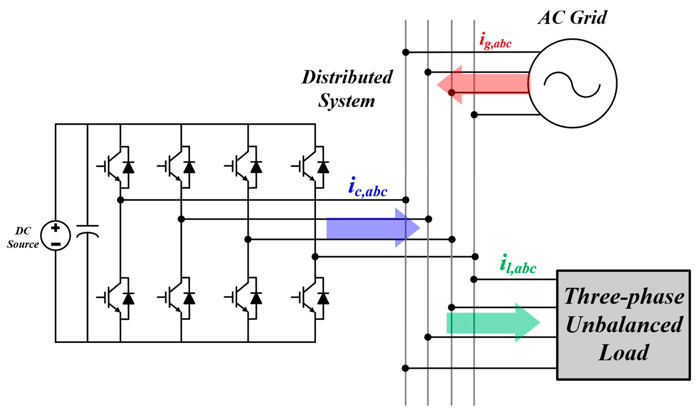
2. Conventional Grid Current Compensation under Unbalanced Load Conditions

Figure 1 illustrates the scenario of an unbalanced load in the system connected to the inverter. When the inverter is not controlled, the load power is entirely supplied by the power grid. Such an unbalanced load causes distortions in the distribution system and deteriorates the overall power quality [25]. Figure 2 shows a vector diagram of the distorted current improved by the inverter. To address these issues, research has been conducted on the LUC method, which compensates for unbalanced loads. When the inverter compensates for the unbalanced loads, the current in the system is balanced. This LUC method comprises two parts: calculating the current reference to compensate for the unbalance current, and the current controller [24]. In this section, we describe the conventional method of calculating the current reference under an unbalanced load. Equation (1) mathematically describes the principle of current compensations.

$${\overrightarrow{i}}_{g,abc}(balanced)={\overrightarrow{i}}_{l,abc}(unbalanced)+{\overrightarrow{i}}_{c,abc}(compensation)$$

(1)

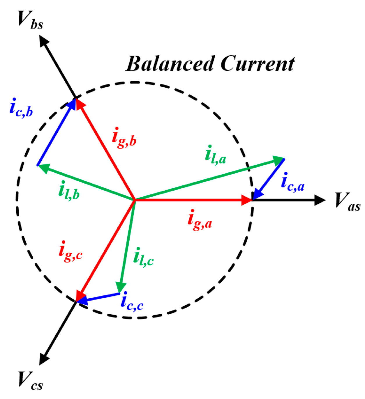
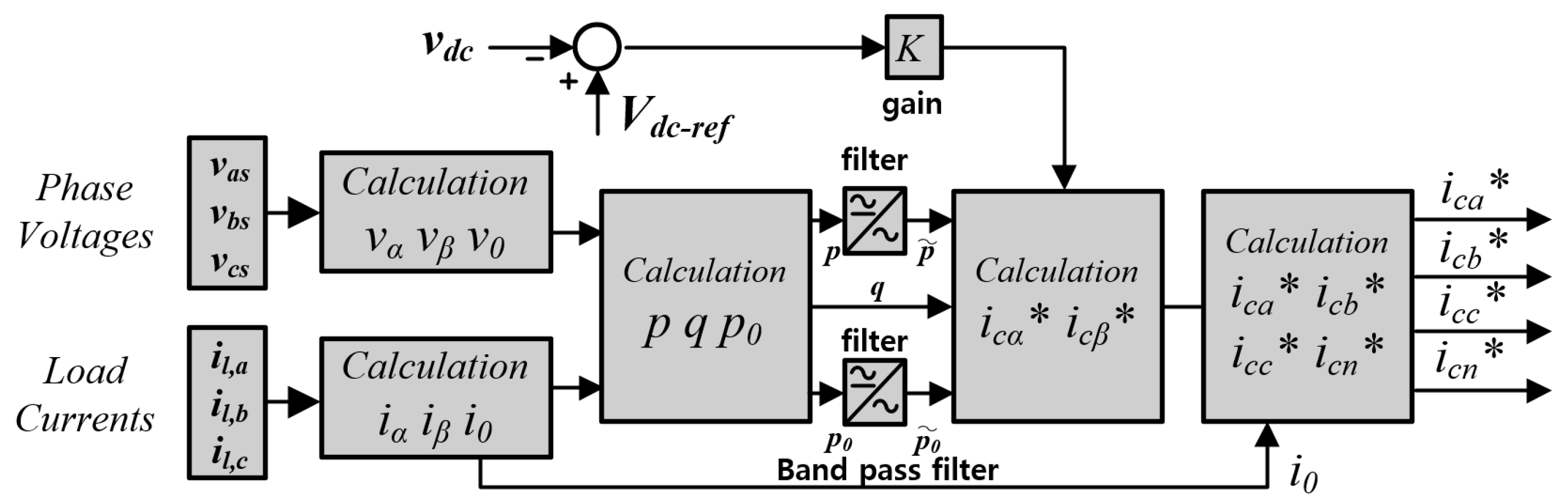
2.1. LUC Based on the P-Q Theory

Figure 3 depicts the block diagram for calculating the current reference based on the instantaneous power p-q theory. Calculations based on the p-q theory remain effective in both the steady and transient states, providing rapid response characteristics even under transient conditions [11]. This method utilizes a band pass filter to compute the current reference using the AC power component. Inputs for the calculation are obtained by transforming the abc coordinates to the stationary coordinates α-β-0, which is represented in Equations (2)–(4) [13].

$$\left[\begin{array}{c}{V}_0\\ V_{\alpha }\\ V_{\beta }\end{array}\right]=\sqrt{\frac{2}{3}}\left[\begin{array}{ccc}1/\sqrt{2}& 1/\sqrt{2}& 1/\sqrt{2}\\ 1& -1/2& -1/2\\ 0& \sqrt{3}/\sqrt{2}& -\sqrt{3}/\sqrt{2}\end{array}\right]\cdot \left[\begin{array}{c}{V}_a\\ V_b\\ V_c\end{array}\right]$$

(2)

$$\left[\begin{array}{c}{i}_0\\ i_{\alpha }\\ i_{\beta }\end{array}\right]=\sqrt{\frac{2}{3}}\left[\begin{array}{ccc}1/\sqrt{2}& 1/\sqrt{2}& 1/\sqrt{2}\\ 1& -1/2& -1/2\\ 0& \sqrt{3}/\sqrt{2}& -\sqrt{3}/\sqrt{2}\end{array}\right]\cdot \left[\begin{array}{c}{i}_a\\ i_b\\ i_c\end{array}\right]$$

(3)

$$\left[\begin{array}{l}p\\ q\end{array}\right]=\left[\begin{array}{l}{v}_{\alpha }\hspace{0.17em}{v}_{\beta }\\ -v_{\beta }\hspace{0.17em}{v}_{\alpha }\end{array}\right]\cdot \left[\begin{array}{l}{i}_{\alpha }\\ i_{\beta }\end{array}\right]$$

(4)

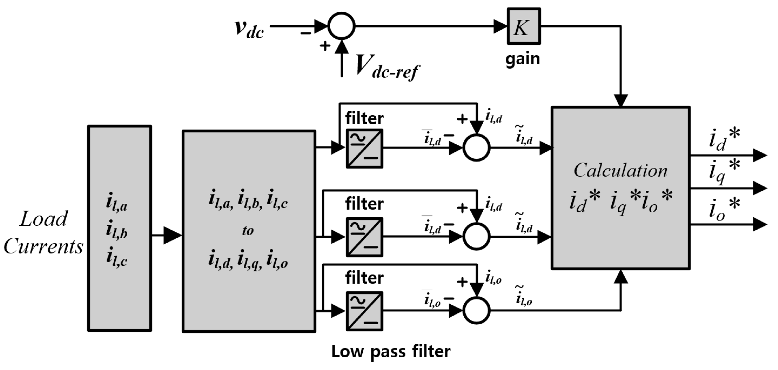
2.2. LUC Based on the Synchronous Frame Theory

Figure 4 illustrates a block diagram for calculating the current reference based on the synchronous reference frame theory. To compute the current reference, the current values must be transformed from the abc coordinates to the dq0 synchronous coordinates. Equation (5) represents the formula for transforming the abc coordinate system into the dq0 coordinate system. When the load is in an unbalanced state, the dq0 current can be expressed by Equation (6). Using this represented current, the unbalanced current reference of the inverter can be computed [26,27]. In Equation (6), the current is divided into DC and AC parts. To obtain a DC current component, an LPF with a very low cut-off frequency must be used. By extracting the constant component of the current through the LPF, the current reference in dq0 coordinates can be calculated using Equation (7). However, the performance of deriving the current reference from an LPF-based synchronous coordinate system is constrained by the time delay introduced by the filter [10,21]. Here, $\overline{i_d},\hspace{0.17em}\hspace{0.17em}\overline{i_q},\hspace{0.17em}\hspace{0.17em}\overline{i_0}$ and ${\tilde{i}}_d,\hspace{0.17em}{\tilde{i}}_q,\hspace{0.17em}{\tilde{i}}_o$ represent the constant and varying parts of the current, respectively.

$$\left[\begin{array}{c}{i}_d\\ i_q\\ i_0\end{array}\right]=\sqrt{\frac{2}{3}}\left[\begin{array}{ccc}\cos \theta & \cos \left(\theta -\frac{2}{3}\pi \right)& \cos \left(\theta +\frac{2}{3}\pi \right)\\ \sin \theta & \sin \left(\theta -\frac{2}{3}\pi \right)& \sin \left(\theta +\frac{2}{3}\pi \right)\\ \frac{1}{2}& \frac{1}{2}& \frac{1}{2}\end{array}\right]\left[\begin{array}{c}{i}_a\\ i_b\\ i_c\end{array}\right]$$

(5)

$$\left[\begin{array}{c}{i}_d\\ i_q\\ i_0\end{array}\right]=\left[\begin{array}{l}\overline{i_d}+{\tilde{i}}_d\\ \overline{i_q}+{\tilde{i}}_q\\ \overline{i_0}+{\tilde{i}}_o\end{array}\right]$$

(6)

$$\left[\begin{array}{c}{i}_d^{\ast }\\ i_q^{\ast }\\ i_0^{\ast }\end{array}\right]=\left[\begin{array}{l}{i}_d-\overline{i_d}\\ i_q-\overline{i_q}\\ i_0-\overline{i_0}\end{array}\right]$$

(7)

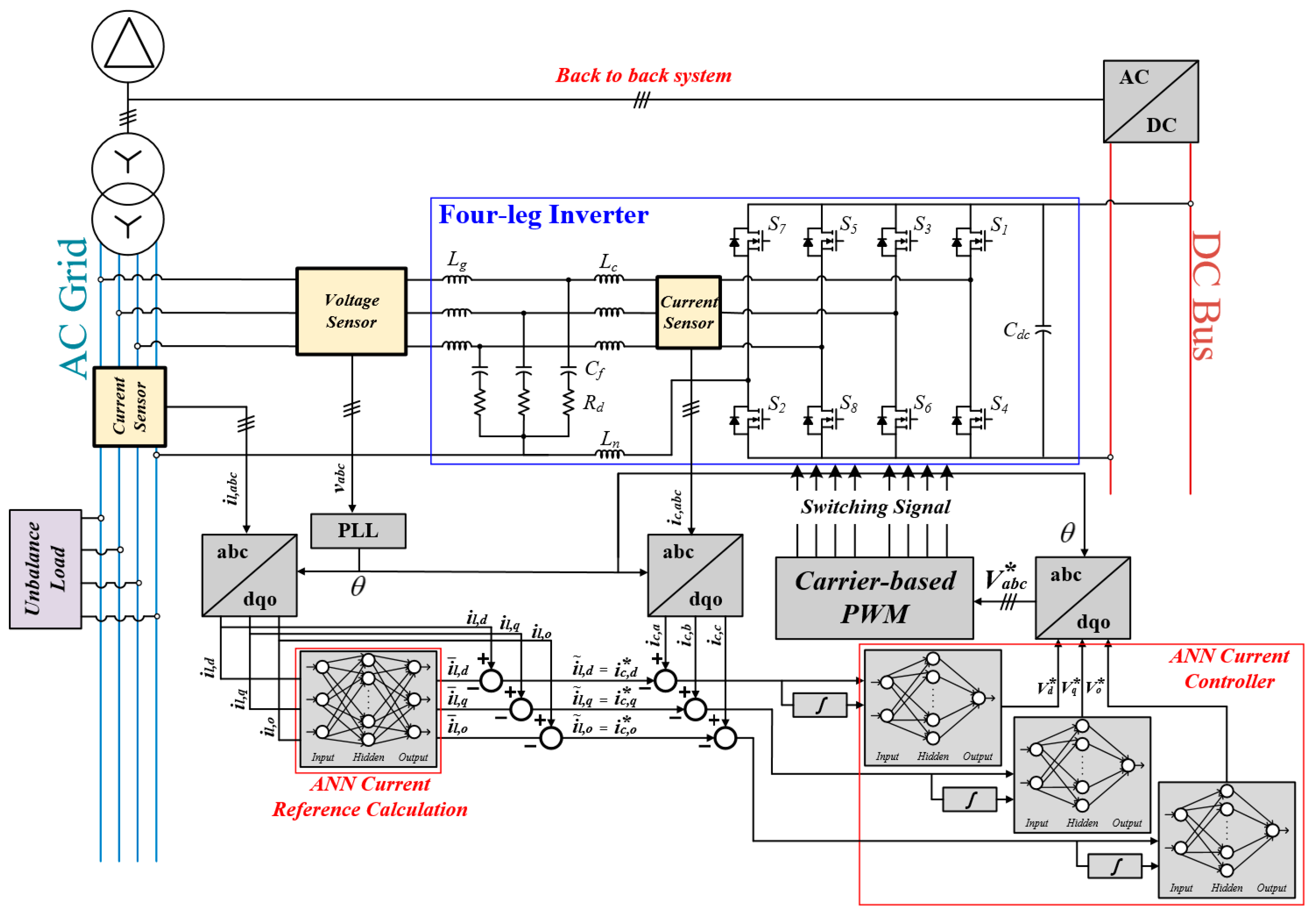
3. Proposed Current Compensation Method Using ANN

Figure 5 shows the control block diagram of the inverter, outlining the proposed approach for compensating the grid current under unbalanced load conditions. Initially, an ANN was devised to calculate the reference current and compensate for the unbalanced current. The ANN was fed with the synchronous coordinate values of the AC current as the input. In addition, three supplementary ANNs were established to control the phase current. A conventional carrier-based pulse width modulation method was employed to govern the inverter, based on the output derived from the ANN training.

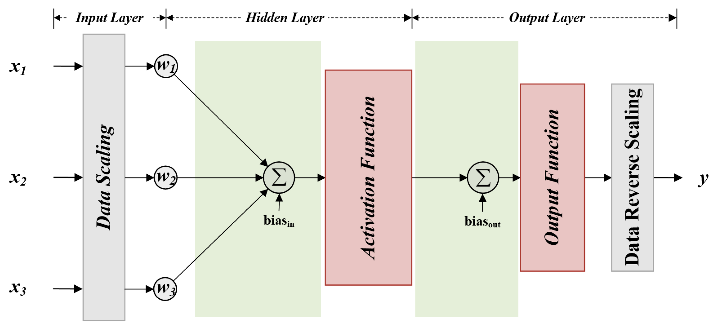
3.1. Designing the ANN Structure using MATLAB

The structure of an ANN is similar to that of a human neural network. The architecture of the ANN applied in this paper is depicted in Figure 6, where $x_k$ represents the input variables; $w_k$ denotes the multiplication weights of the ANN; the activation function, the output function, and the bias represent the addition weights of the ANN; and y signifies the output value.

The ANN consists of three layers: the input, the hidden, and the output layers. The output of the activation function is formulated as the product and sum of the inputs, as expressed in the following equation, where $x_{\mathrm{k,min}}$, $x_{\mathrm{k,max}}$, $y_{\min }$, and $y_{\max }$ are the minimum and maximum values of each sample of training input and output data, respectively.

$$y=\frac{y_{\max }-y_{\min }}{2}\left[f\left[\left\{2\left(\frac{x_1-x_{1,\min }}{x_{1,\max }-x_{1,\min }}\right)-1\right\}{w}_1+\left\{2\left(\frac{x_2-x_{2,\min }}{x_{2,\max }-x_{2,\min }}\right)-1\right\}{w}_2+\left\{2\left(\frac{x_3-x_{3,\min }}{x_{3,\max }-x_{3,\min }}\right)-1\right\}{w}_3+bia{s}_{in}\right]+bia{s}_{out}\right]+y_{\min }$$

(8)

The activation function outputs large values for inputs above a certain threshold, without outputting small values. Owing to the characteristics of each activation function, they typically output values between 0 and 1 or between −1 and 1, necessitating the scaling of the input and output data. Although various activation functions exist, the three most commonly used functions include the sigmoid, the rectified linear unit (ReLU), and the hyperbolic tangent functions, which are represented in Figure 7.

The reason for using nonlinear activation functions is to solve the problems of the model more effectively. When using linear functions, the presence of hidden layers may result in unnecessary outcomes because the relationship between the inputs and outputs is merely represented by addition and multiplication. Therefore, the activation functions must be non-linear. However, for the output function, it is necessary to reflect data passing through the hidden layers of the output. However, the application of a non-linear function to an output function may lead to data loss. In this study, we applied a sigmoid function as the activation function, which is reflected in the simulation results presented in the following section [28]. The MATLAB R2020b toolbox used to train the ANN applied in the paper was validated through three steps.

(1)

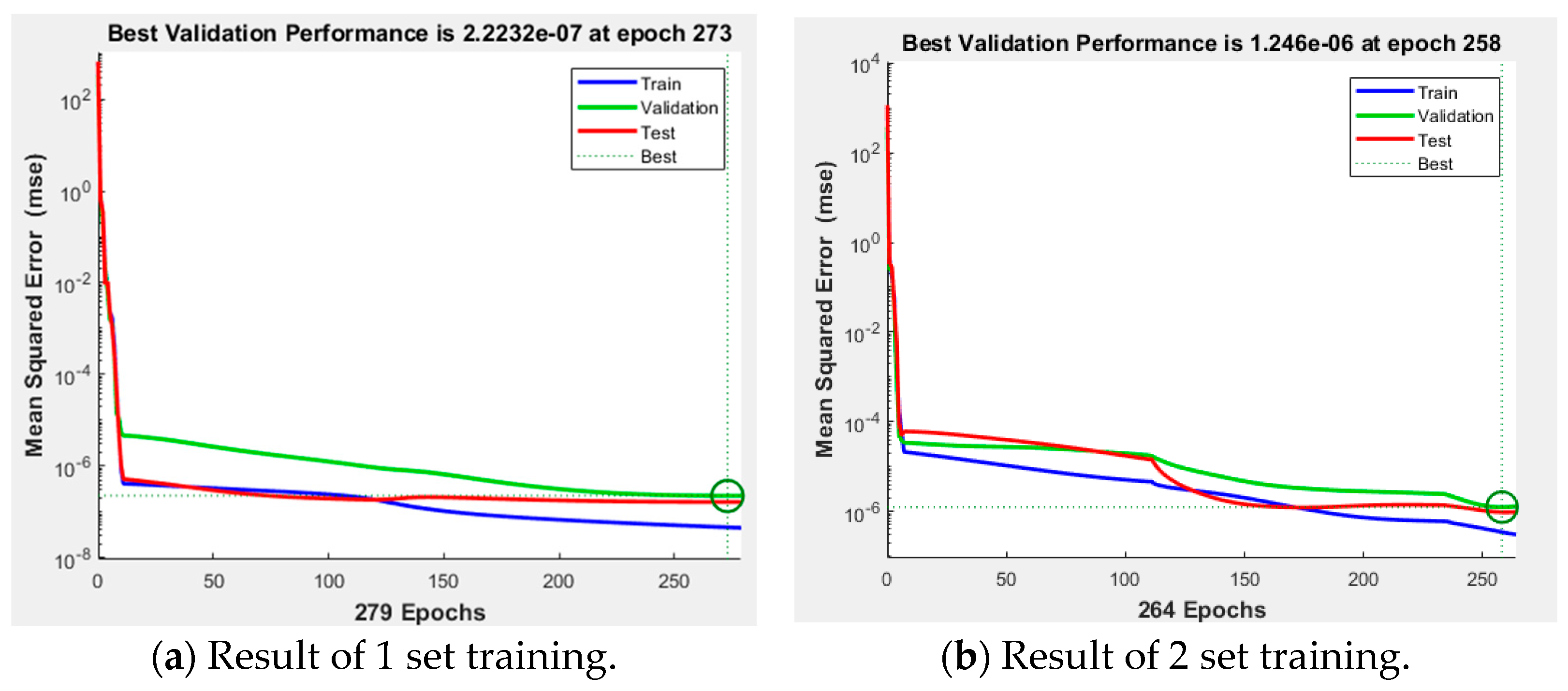
Step 1: training data ratio validation

In this study, MATLAB’s Neural Fitting (nftool), from MathWorks, was utilized for the ANN training, and the structure of the ANN was configured as shown in Figure 8. When using the training toolbox, the user can select the ratio of training data, validation data to monitor the training progress, and testing data to evaluate the performance of the trained ANN. In this study, 100 test datasets for the q-axis current controller were used to determine the data sample ratio. The results are presented in

Table 1. Result of training data ratio based on the q-axis current controller dataset.

		Samples (%)	MSE (Mean Square Error)	R
1 Set	Training	70	4.55392 × 10−8	9.99999 × 10−1
	Validation	15	2.22321 × 10−7	9.99999 × 10−1
	Testing	15	1.63285 × 10−7	9.99999 × 10−1
2 Set	Training	90	3.44847 × 10−7	9.99999 × 10−1
	Validation	5	1.24599 × 10−6	9.99999 × 10−1
	Testing	5	9.57606 × 10−7	9.99999 × 10−1

and Figure 9, where it can be observed that the presence of appropriate ratios of validation and testing data is essential for achieving high accuracy.

(2)

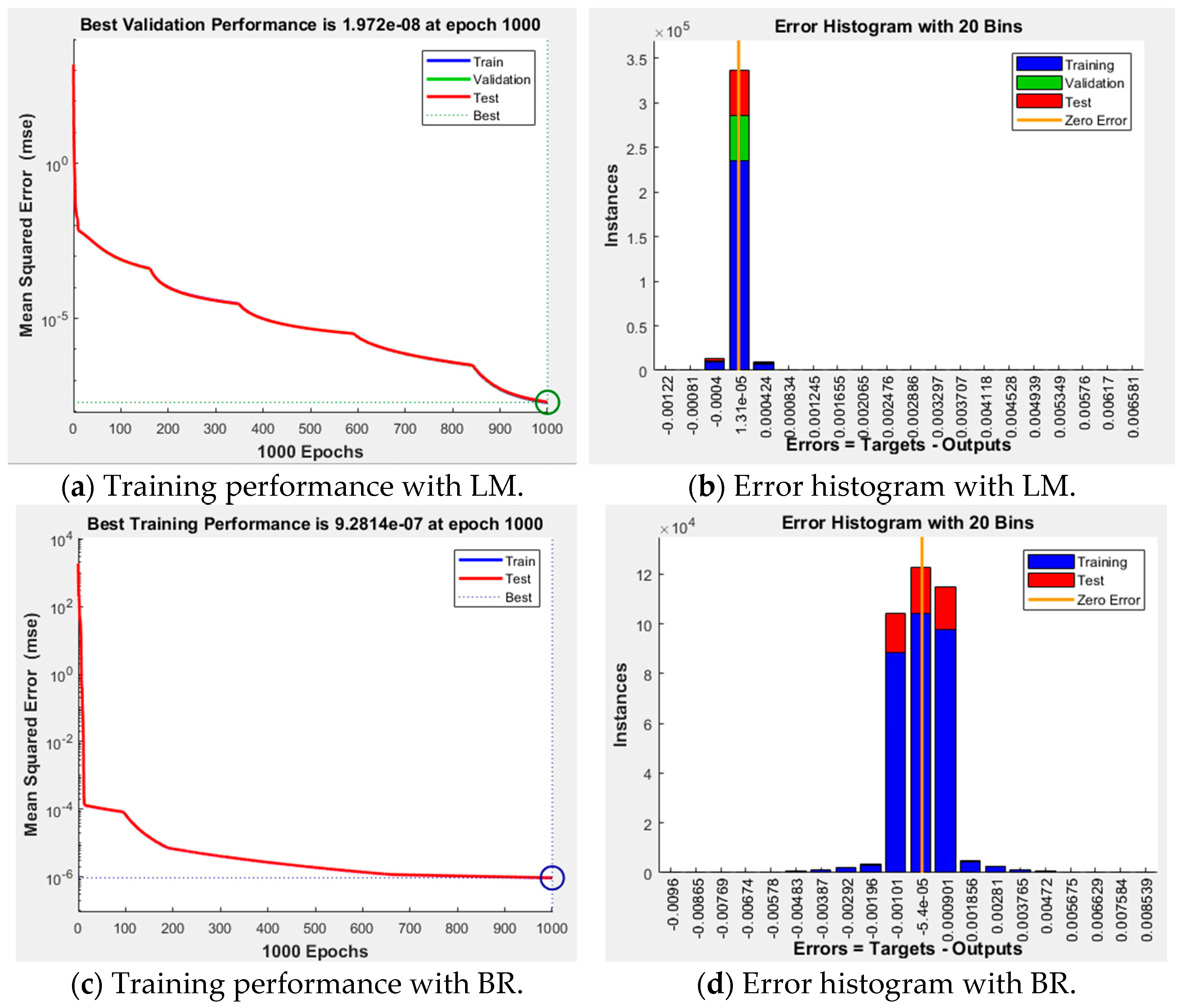
Step 2: training algorithm validation

Based on previous results, the ratio of the test data was configured as follows: training 70%, validation 15%, and testing 15%. In this study, ANN was trained using the backpropagation method, and MATLAB provided three algorithms: the Levenberg–Marquardt (LM) algorithm, Bayesian regularization (BR), and the scaled conjugate gradient (SCG) method, which can be summarized as follows:

-

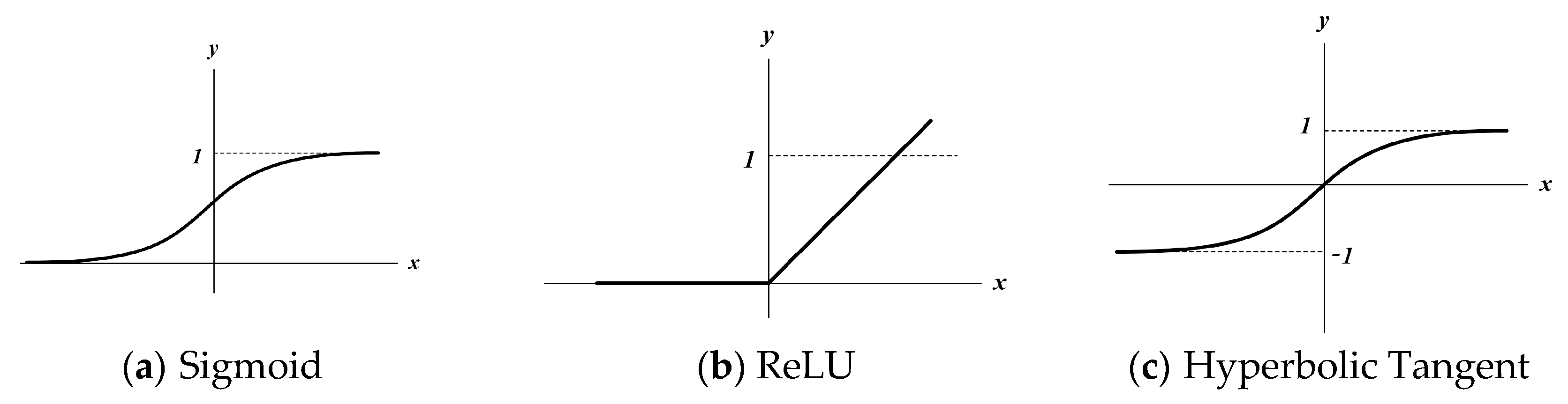
Levenberg–Marquardt algorithm: The LM method combines the Gauss–Newton and gradient descent methods to efficiently determine both global and local minima. Although this offers both stability and faster convergence, it requires significant computational effort to determine initial values when they are not provided.

-

Bayesian regularization: This method trains a neural network to minimize errors only for the provided training data, which may lead to over-confidence. Although BR considers uncertainty and enhances robustness against noise or inputs beyond the training data, it tends to have a slower convergence. Additionally, it may produce different outputs for the same parameters owing to its consideration of uncertainty.

-

Scaled conjugate gradient method: Introduced by Moller, the SCG method differs from other conjugate gradient algorithms in that it does not recalculate at each iteration and performs backpropagation with a second-order approximation of the error. This approach ensures the robustness and independence of the neural network from user-defined training data. However, the approach is complex and requires substantial computational resources and training times.

Figure 10 depicts the results of training the ANN current controller using three algorithms supported by MATLAB. All simulations involved 1000 iterations of identical training using the q-axis current controller dataset. When comparing the training performance and error histograms, as shown in

Table 2. Comparison of ANN training algorithms—Epoch 1000.

	Training Performance	Error Histogram
Levenberg–Marquardt	1.972 × 10−8	1.31 × 10−5
Bayesian Regularization	9.2814 × 10−7	−5.4 × 10−5
SCG Method	0.0048582	−0.1241

, it is observed that the LM training algorithm exhibits the least amount of error.

(3)

Step 3: number of neural validations

Figure 11 illustrates the training performance and error histogram based on the number of hidden neurons in the ANN using the q-axis current controller dataset. The training performance of the ANN with 30 hidden neurons is superior; however, the error histogram of the ANN with 20 hidden neurons indicates that the majority of errors are dominantly distributed in one area. Such dominant errors make it easier to compensate for the results of the ANN through the feedforward method. Based on the simulation results, we applied an ANN with 20 hidden neurons trained using the LM method.

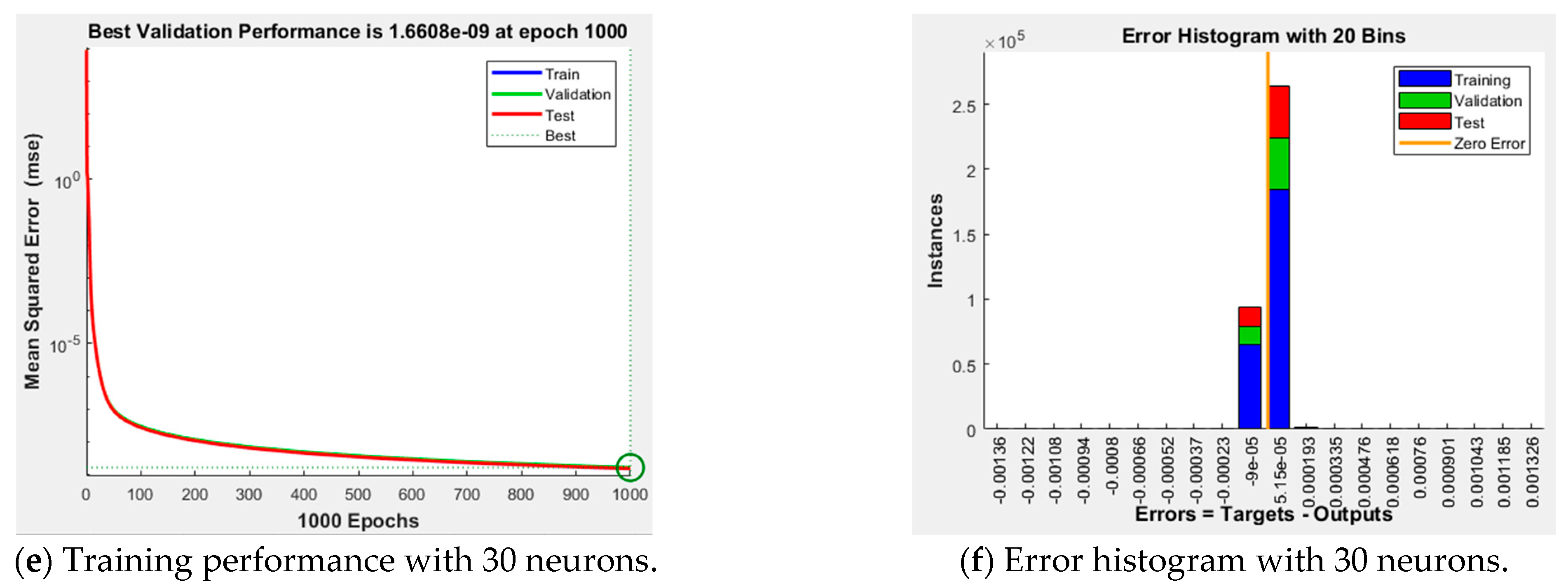
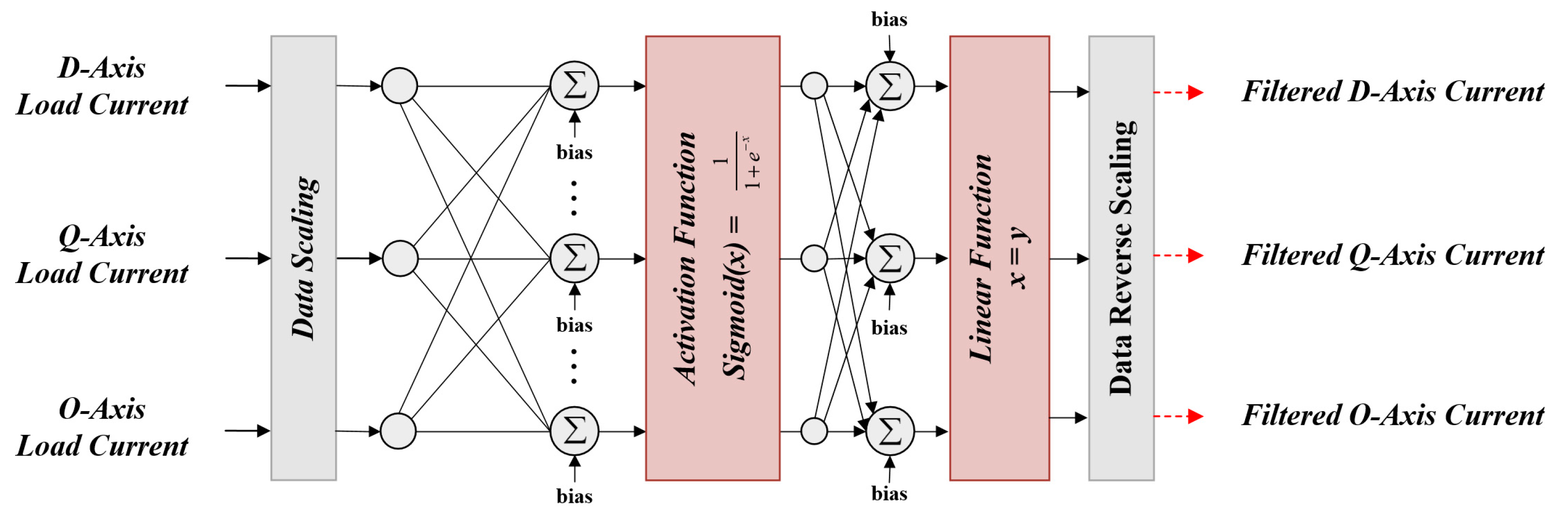
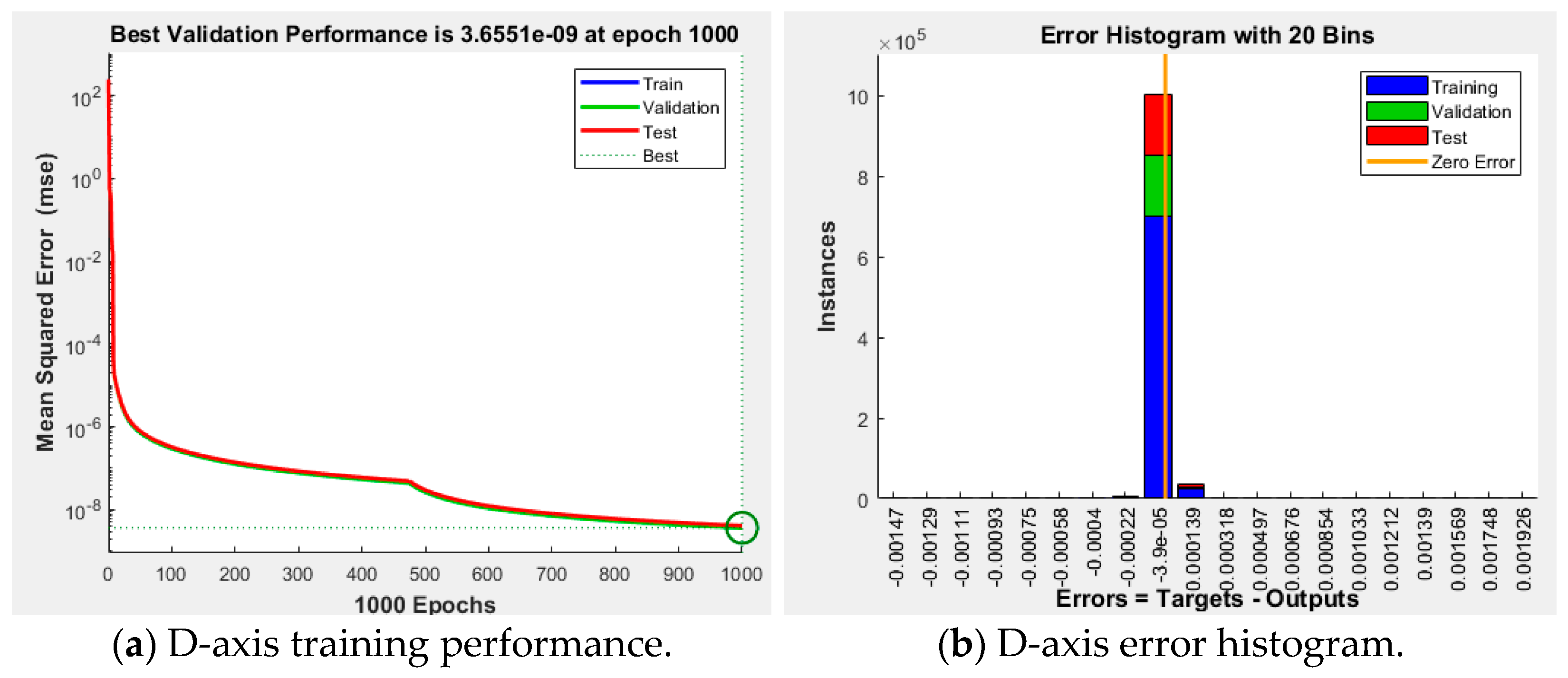
3.2. Designing an ANN for the Calculation of Current Reference under Unbalanced Load Conditions

The structure of the ANN for calculating the current reference in the case of load unbalance is illustrated in Figure 12. The ANN input consisted of the dq0 axis synchronous reference frame currents of the load, while the output wass composed of the average values of the unbalanced magnitudes in the dq0 axis. The ANN was configured using three inputs, three outputs, and 20 hidden neurons. Figure 13 shows the training results of the ANN for unbalance calculation.

Table 3. ANN training data summary of current reference calculation.

Input Data			Output Data
Ide	Iqe	Ioe	Ide_ref	Iqe_ref	Ioe_ref
−0.881433331	−9.342378775	−0.181107398	−6.01 × 10−1	−10.781192	0.000155916
−0.661866636	−9.316670329	−0.070921802	−6.01 × 10−1	−10.781192	0.000155916
−0.440898051	−9.324221858	0.039687159	−6.01 × 10−1	−10.781192	0.000155916
……
−2.942782404	−9.855400085	−1.241158981	−0.77460625	−13.886127	0.000126828
−2.312665572	−9.575398404	−0.905744661	−0.77460625	−13.886127	0.000126828
−1.647599185	−9.393269653	−0.565187099	−0.77460625	−13.886127	0.000126828

summarizes the approximately 40,000 samples of data used to train the ANN.

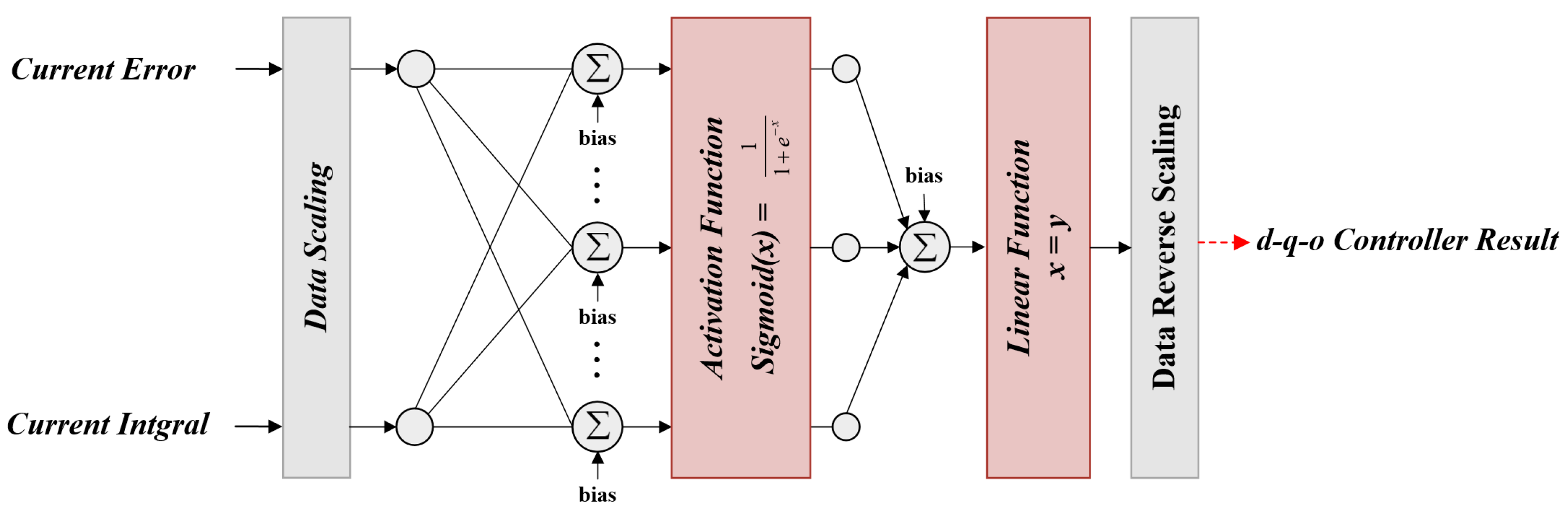
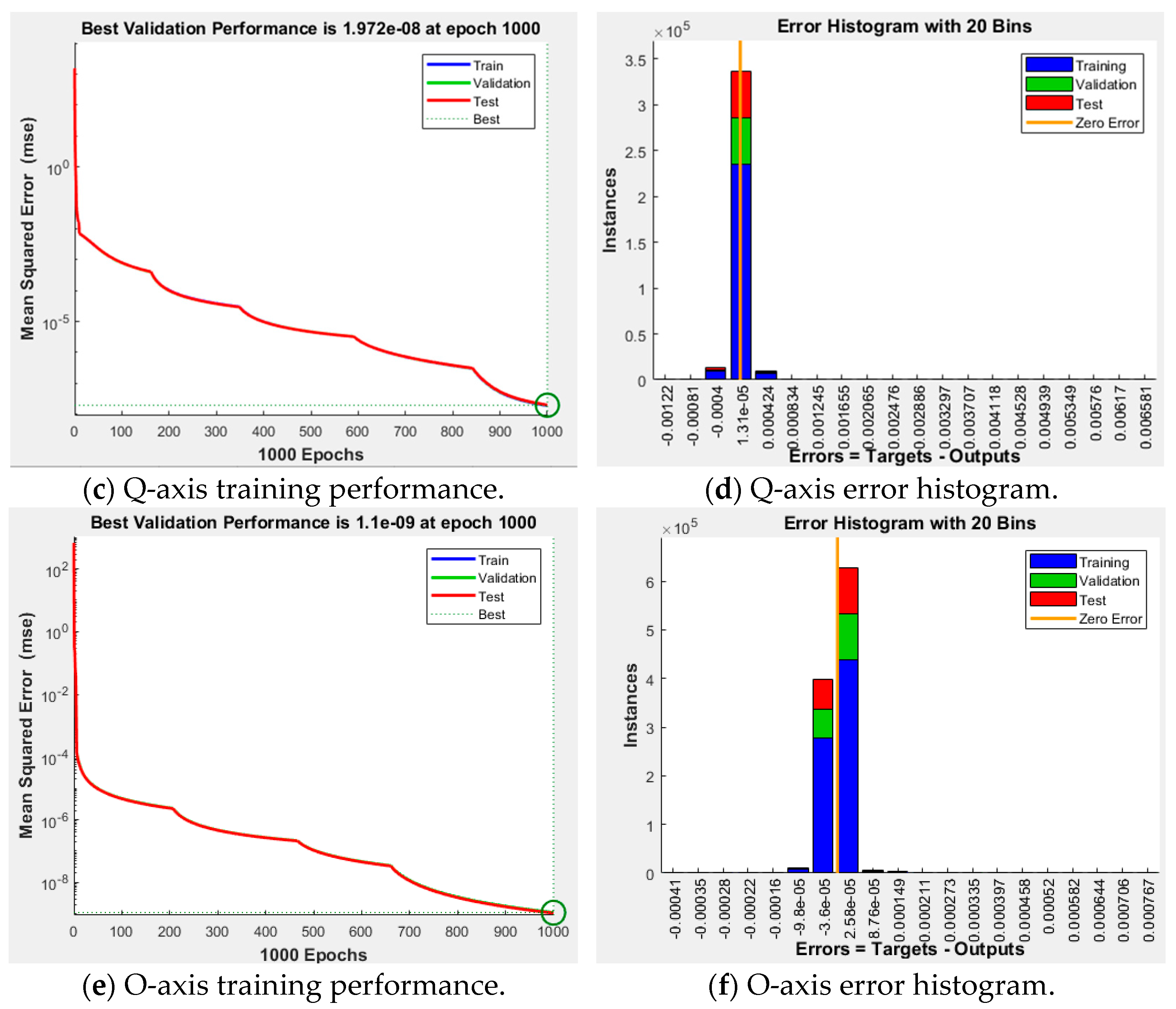
3.3. Designing an ANN for the Current Controller in the dq0 Axis

The structure of the ANN for the dq0 axis current controller in the case of a load unbalance is illustrated in Figure 14. The input of the ANN consists of the proportional and integral error values of each axis, whereas the output is composed of the PI controller of each axis. The ANN was configured with two inputs, one output, and 20 hidden neurons. Figure 15 shows the training results of the ANN for the current controller of each axis.

Table 4. ANN training data summary of the current controller.

Input Data						Output Data
Error D-Axis	Integral D-Axis	Error Q-Axis	Integral Q-Axis	Error O-Axis	Integral O-Axis	D-Axis	Q-Axis	O-Axis
0.065365	12.41371	−0.0188	−358.686	0.074611	0.390667	13.72101	−359.062	1.882889
0.07662	12.5265	−0.0413	−358.738	0.034672	0.45742	14.05891	−359.564	1.150865
0.041886	12.50608	−0.04018	−358.977	0.038226	0.616964	13.34381	−359.781	1.38149
∙ ∙ ∙ ∙
0.059906	12.49728	−0.07878	−358.877	0.076294	0.651035	13.69541	−360.452	2.176914
0.06789	12.1754	0.006137	−358.662	−0.04231	−0.22027	13.53321	−358.54	−1.06654
−0.00376	11.72399	0.075598	−359.193	−0.06424	0.526357	11.64879	−357.681	−0.75839

summarizes approximately 85,000 samples of each axis of the data used to train the ANN.

Table 5. Summary of ANN learning results.

	Training Performance	Dominant Error Histogram
Unbalance calculation	0.0091582	−0.04391
d-axis controller	3.6551 × 10−9	−3.9 × 10−5
q-axis controller	1.972 × 10−8	1.31 × 10−5
o-axis controller	1.19 × 10−9	2.58 × 10−5

summarizes the training results of the ANN conducted in this paper.

4. Simulation Results

Simulations were performed using the PSIM 9.1.4 program to validate the effectiveness of the proposed method. Three simulation cases are considered to conduct a comparative analysis using the conventional method. The initial case involved the application of the LPF-based dq0 reference generation and the PI current control. In the second case, an ANN-based dq0 reference generation, coupled with a PI controller, was incorporated. Finally, the proposed approach utilized an ANN-based dq0 reference generation and an ANN current controller for simulation. Figure 16 illustrates the configuration of the applied simulation and experimental setups. The parameters of the four-leg inverter and the load applied in the simulations and experiments are listed in

Table 6. Parameters of the simulation and experiment.

Parameters		Values	Unit
Grid Line to Line Voltage		220	$V_{rms}$
DC-Link Voltage		380	$V_{dc}$
AC Load	A Phase	1.014	kW
	B Phase	0.69	kW
	C Phase	0.69	kW
Inverter Rated Power		20	kW
LCL Filter	Grid Inductance	100	μH
	Filter Capacitance	22	μF
	Converter Inductance	1500	μH
DC-Link Capacitance		1200	μF

. The unbalance loads for each phase are listed in Table 6, and the voltages and currents before the compensation are shown in Figure 17.

4.1. Case 1 (LPF-Based dq0 Reference Generation and PI Current Controller)

The conventional method employs a synchronous reference frame LPF-based current reference calculation. This approach calculates the magnitude of the unbalance value using an LPF and compensates for the unbalanced current using an inverter with a PI current controller. Figure 18 shows the simulation waveforms obtained using the conventional method. At time $t_1$, a load is applied during the simulation, and at time $t_2$, the load is removed. The load was applied with 1.014 kW in phase A, 0.69 kW in phase B, and 0.69 kW in phase C, making an unbalanced current situation. The waveform depicts the current in the distribution system and the compensating phase current provided by the inverter. The next waveform represents the magnitude of the unbalance component calculated using the LPF. The final simulation waveform depicts the current reference for the compensation performed by the inverter. The simulation waveform on the left represents the situation in which the system transitions from a no-load to a moderate load condition, while the simulation waveform on the right represents the situation in which the system transitions from a loaded state to a no-load condition. The first waveform in Figure 18 represents the grid current under unbalanced load conditions. This current slowly follows the load variations owing to the delay in determining the unbalance magnitude using the LPF, as depicted in the third plot. When transitioning from a no-load to a loaded condition, it takes 0.125 s to reach an average q-axis current value of −10.788 in a steady state. Similarly, when transitioning from a loaded to a no-load condition, it takes 0.1 s to reach a steady state. Figure 19 shows enlarged waveforms of points A and B in Figure 18. The ripple magnitudes and total harmonic distortion (THD) of each phase current are listed in

Table 7. Maximum ripple and THD of phase currents in the transient state owing to load fluctuations in Case 1.

		A Phase	B Phase	C Phase	Average
Point A [A]	Grid	16.43	12.52	3.52	10.82
	Inverter	4.67	9.02	6.85	6.85
Point B [A]	Grid	-	16.79	15.24	16.02
	Inverter	-	11.31	10.62	10.97
THD [%]	Grid	3.365	3.409	3.451	3.41
	Inverter	5.637	12.21	10.852	9.57

. However, for Point B, the ripple in the phase A current is negligible and is thus not indicated separately.

Such delays are unsuitable for distribution systems in which loads continuously fluctuate. To address this issue, an ANN was applied to the dq0 reference generation in the inverter, reducing the time required for compensation to reach a steady state.

4.2. Case 2 (ANN dq0 Reference Generation and PI Current Controller)

In Case 2, unlike in Case 1, the synchronous reference LPF-based current reference calculation was performed using an ANN. The current controller used the same PI current controller as that employed in Case 1. In the simulation, the load transitioned from no load to load at $t_1$, and from load to no load at $t_2$, as in Case 1. The load values were also the same as in Case 1, with 1.014 kW in phase A, 0.69 kW in phase B, and 0.69 kW in phase C. The simulation waveforms shown in Figure 20 are arranged in a manner similar to that in Case 1; however, the third waveform represents the magnitude of the unbalanced current calculated by the ANN. Figure 21 shows enlarged waveforms of points A and B from Figure 20. The maximum ripple magnitude and THD for each current are listed in

Table 8. Maximum ripple and THD of phase currents in the transient state due to load fluctuations in Case 2.

		A Phase	B Phase	C Phase	Average
Point A [A]	Grid	19.09	11.51	8.34	12.98
	Inverter	9.11	9.61	4.08	7.6
Point B [A]	Grid	-	21.61	23.05	22.33
	Inverter	-	12.82	12.2	12.51
THD [%]	Grid	5.385	6.809	5.595	5.93
	Inverter	9.41	30.24	28.11	22.59

. Similar to Case 1, for Point B, the ripple in the phase A current is negligible and is thus not indicated separately.

Instead of the synchronous reference LPF-based current reference calculation, applying an ANN significantly reduces the transition time from no-load to load conditions. Specifically, the time to reach the steady state decreases from 0.125 s to 1.7 ms, which is 73.5 times faster when transitioning from no-load to load conditions. Similarly, when transitioning from load to no-load conditions, the time reduces from 0.1 s to 1.76 s, which is 56.82 times faster for reaching the steady state. The simulation results revealed the following outcomes. The MSE for calculating the dq0 commands using an ANN was found to be exceedingly low. However, owing to the error and integral value changes in the PI current controller, unlearned input values distort the output of the ANN every 8.5 ms. Consequently, this decreases the THD of the currents in the inverter and grid. However, this problem arises because the periodic occurrence of the incorrect ANN output leads to an overall increase in the phase current ripple in both the grid and inverter. This ripple increase resulted in deteriorated THD levels. The outcomes of this study are presented in Table 8. Ultimately, at Point A, the average maximum ripple in the grid increased by 1.2 times, and for the inverter current, it increased by 1.12 times. At Point B, the average maximum ripple in the grid increased by 1.39 times, and for the inverter current, it increased by 1.14 times. The THD was calculated to be 1.74 times higher than the average current distortion at Point A and 2.36 times higher at Point B. In the no-load condition, the ANN unbalance calculation outputs values close to zero for the d, q, and o currents. In addition to these training results, considering that the three inputs (the dq0 axis currents) determine the three outputs (dq0 axis current references), all three values include AC components, resulting in a slight time delay in outputting the DC component values.

Combining the conventional PI current controller with the ANN reference calculation resulted in a reduction in the transient states. However, the average maximum ripple and current average THD decreased. To mitigate this periodic distortion, a separately trained ANN-based current controller, which learned the repeated incorrect output and transients of the ANN, was applied in Case 3.

4.3. Case 3 (ANN dq0 Reference Generation and ANN Current Controller)

In Case 3, both ANN-based reference calculations and current controllers were applied. The ANN-based current controller applied in Case 3 was trained to address the repetitive incorrect outputs of the ANN observed in Case 2, along with the transient and steady states, based on the PI current controller. Case 3 also applied the same load magnitude at the same time as in Cases 1 and 2 to compare the transient states at the same point in time. Figure 22 and Figure 23 represent the simulation results for Case 3, with a simulation setup identical to that of Case 2. The maximum ripple magnitude and THD for each current are listed in

Table 9. Maximum ripple and THD of phase currents in the transient state due to load fluctuations in Case 3.

		A Phase	B Phase	C Phase	Average
Point A [A]	Grid	7.08	3.03	0.49	3.53
	Inverter	4.43	4.12	0.65	3.07
Point B [A]	Grid	-	5.23	5.28	5.26
	Inverter	-	4.32	4.22	4.27
THD [%]	Grid	3.46	3.44	3.5	3.47
	Inverter	6.16	12.8	14.1	11.02

. Similar to the previous cases, for Point B, the ripple in the phase A current is negligible, and is thus not indicated separately.

The time required for the current reference calculation to reach a steady state, based on the ANN, was confirmed through simulations to be the same as that in Case 2. As shown in Table 8, when the ANN and PI current controllers were applied, the maximum ripple and THD of the current deteriorated significantly. However, with the improvement achieved by the ANN current controller, compared to Case 1, the maximum ripples of the grid at points A and B decreased by 3.05 times and 2.57 times, respectively. For the inverter currents, they decreased by 3.06 times and 2.23 times, respectively, at each point. Simulation results confirm that compared to Case 2, the THD of both the grid and inverter currents improved by 1.71 times and 2.05 times, respectively, approaching a performance level similar to that of Case 1 in terms of THD.

Table 10. Comparison of simulation average results for the three cases.

		Case 1	Case 2	Case 3
Point A maximum ripple [A]	Grid	10.82	12.98	3.53
	Inverter	6.85	7.6	3.07
Point B maximum ripple [A]	Grid	16.02	12.33	5.26
	Inverter	10.97	12.51	4.27
Average THD [%]	Grid	3.41	5.93	3.47
	Inverter	9.57	22.59	11.02
Average steady state reaching time [s]		0.1125	0.00173	0.00173

summarizes the average values of the three cases and compares their overall performance. The simulation results indicate that Case 3, which applies the proposed method, is advantageous for distribution system applications.

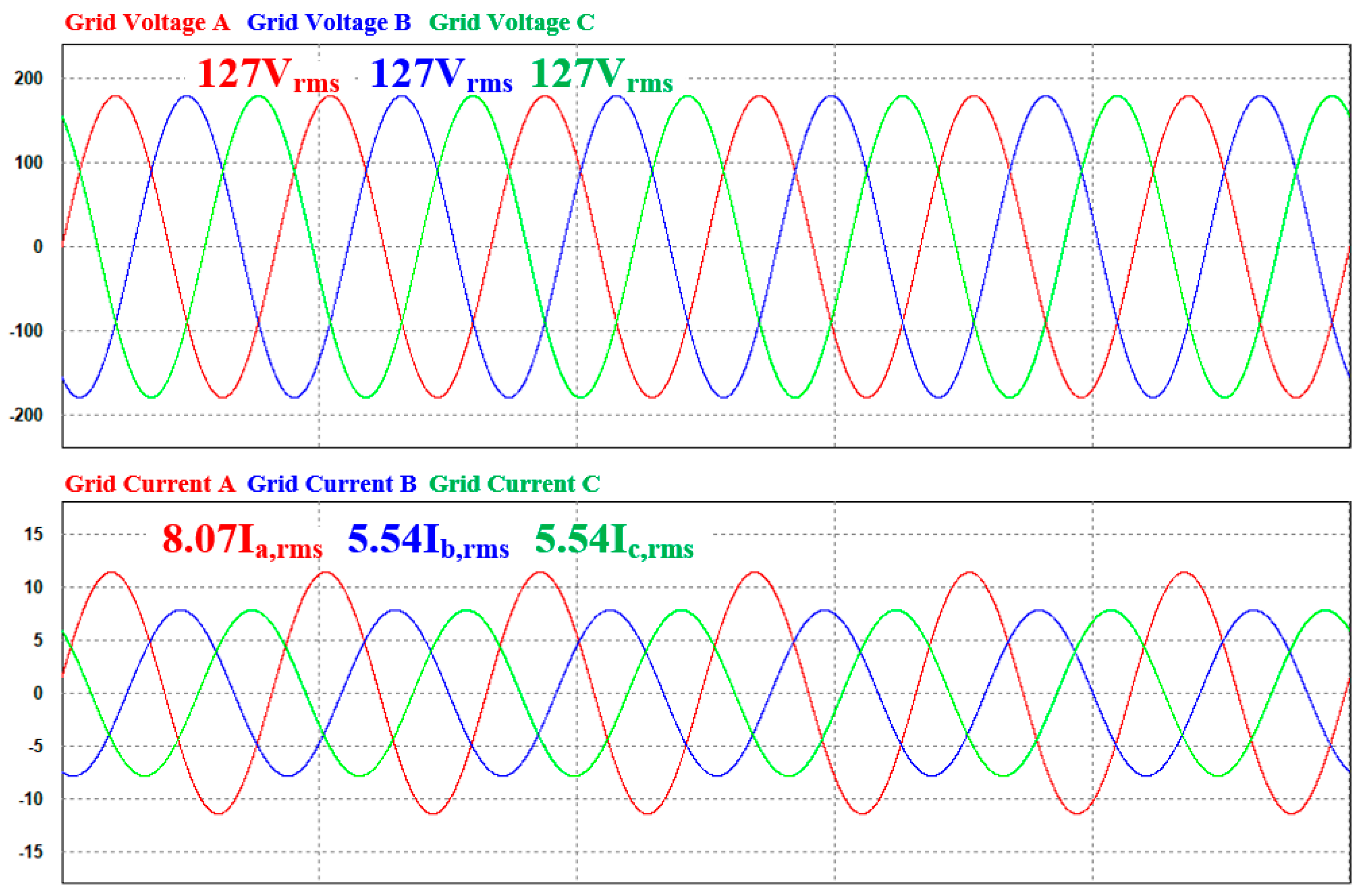
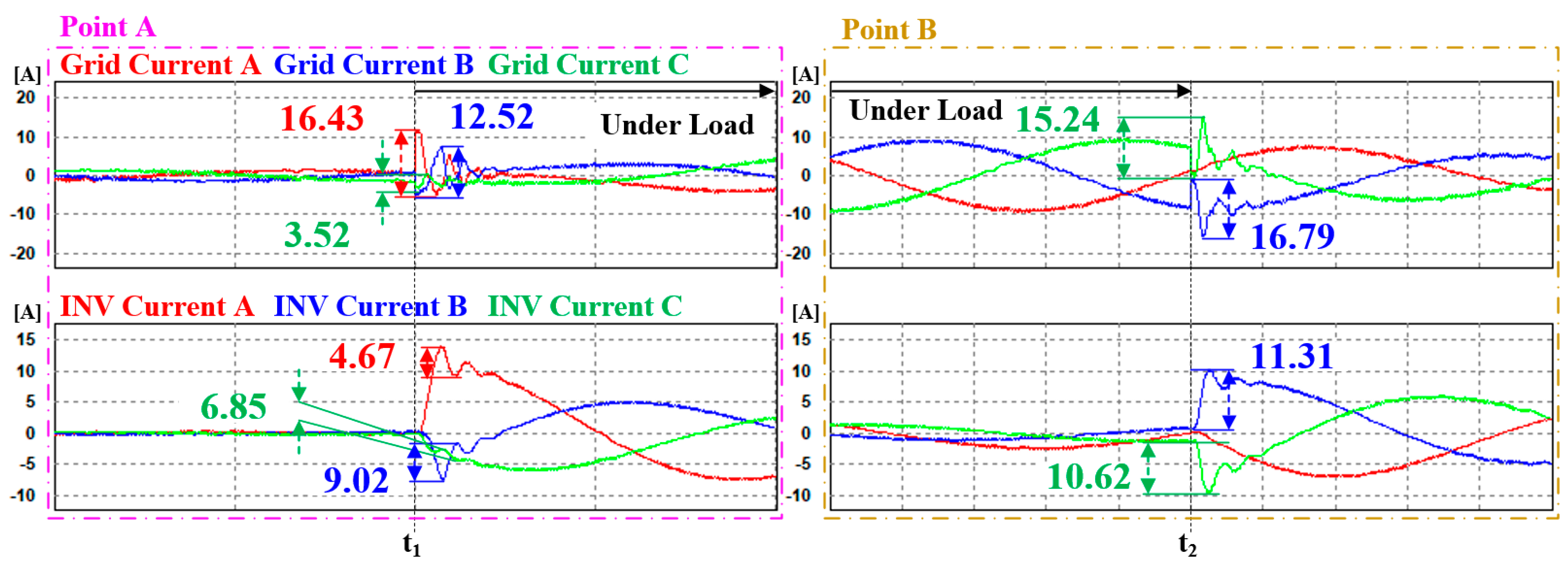
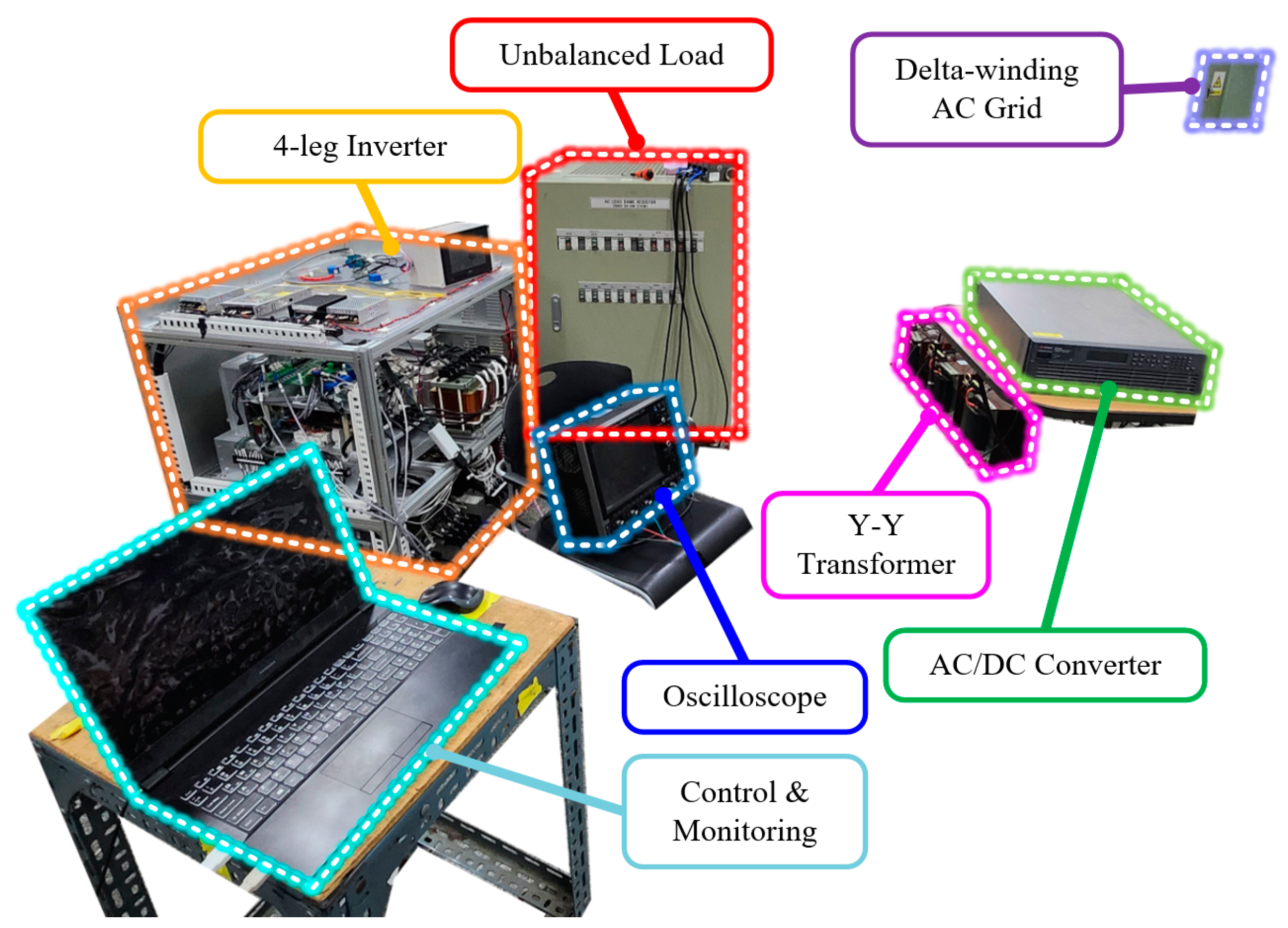
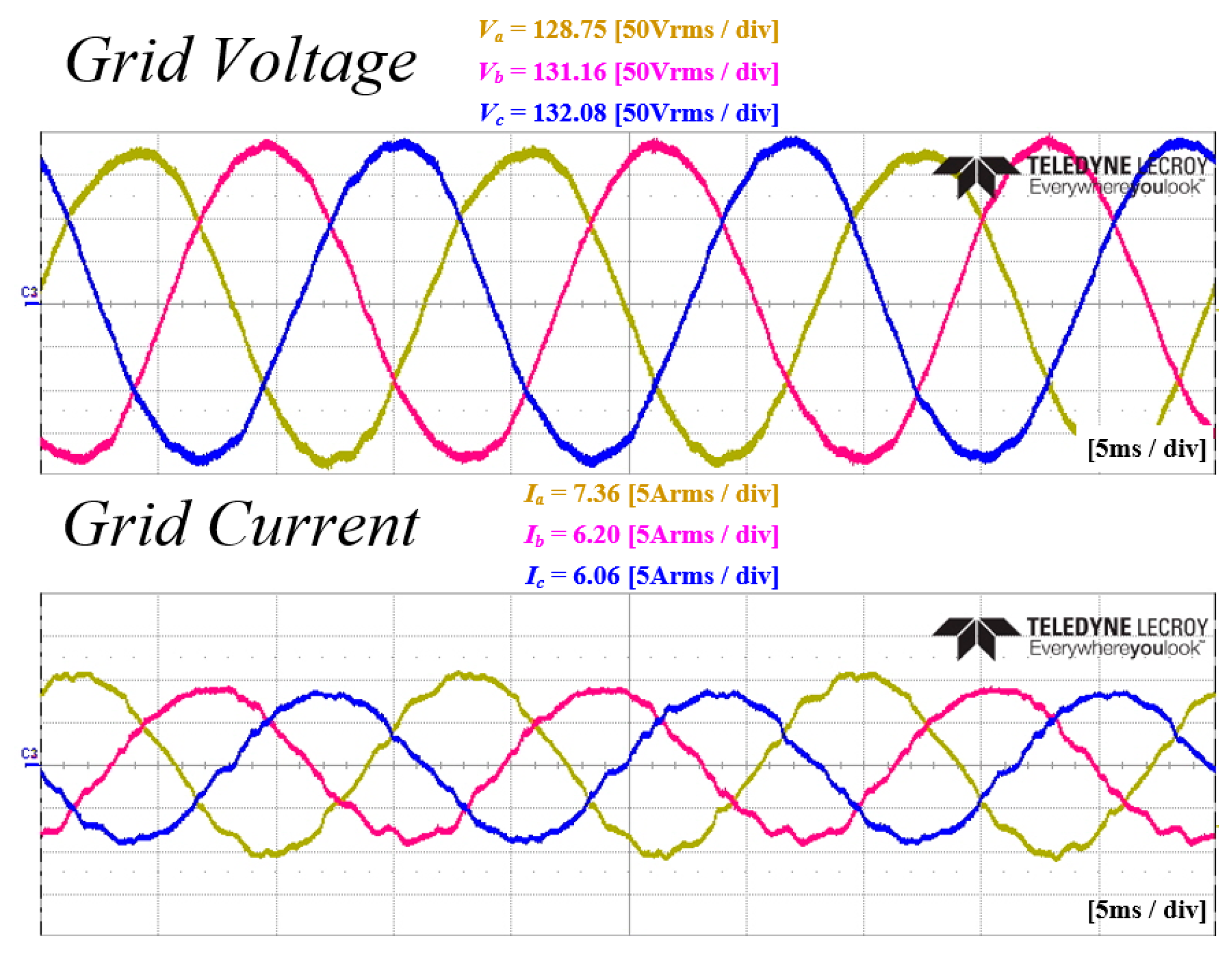
5. Experimental Results

Figure 24 shows the experimental configuration used to verify the proposed ANN-based compensation method under unbalanced load conditions. The parameters of the three-phase the four-leg inverter and the three-phase unbalanced resistance load are listed in Table 6. In the experiment, the current compensation method was applied to a four-leg inverter in a distributed system under unbalanced load conditions using an ANN.

The experiments were conducted in three cases, similar to the method used in the simulations. The AC voltage was maintained by the grid, while the DC voltage was controlled by the AC/DC converter connected in a back-to-back system linking to a delta-winding grid. The laboratory grid was in a delta-winding configuration, so three single-phase transformers were connected in a Y-Y configuration to perform the four-wire experiments. The experiments were conducted only on the no-load to loaded state sequence. Figure 25 depicts the voltage and current waveforms of the secondary side of the Y-Y transformer. Since the experiments were conducted in the laboratory, the grid was limited to the operation of the unbalanced experiments, and there is slight distortion in the voltage due to the presence of harmonics caused by the characteristics of the Y-Y transformer. The switching frequency of the four-leg inverter is 10 kHz, and the control period is 5 kHz, with experiments conducted accordingly.

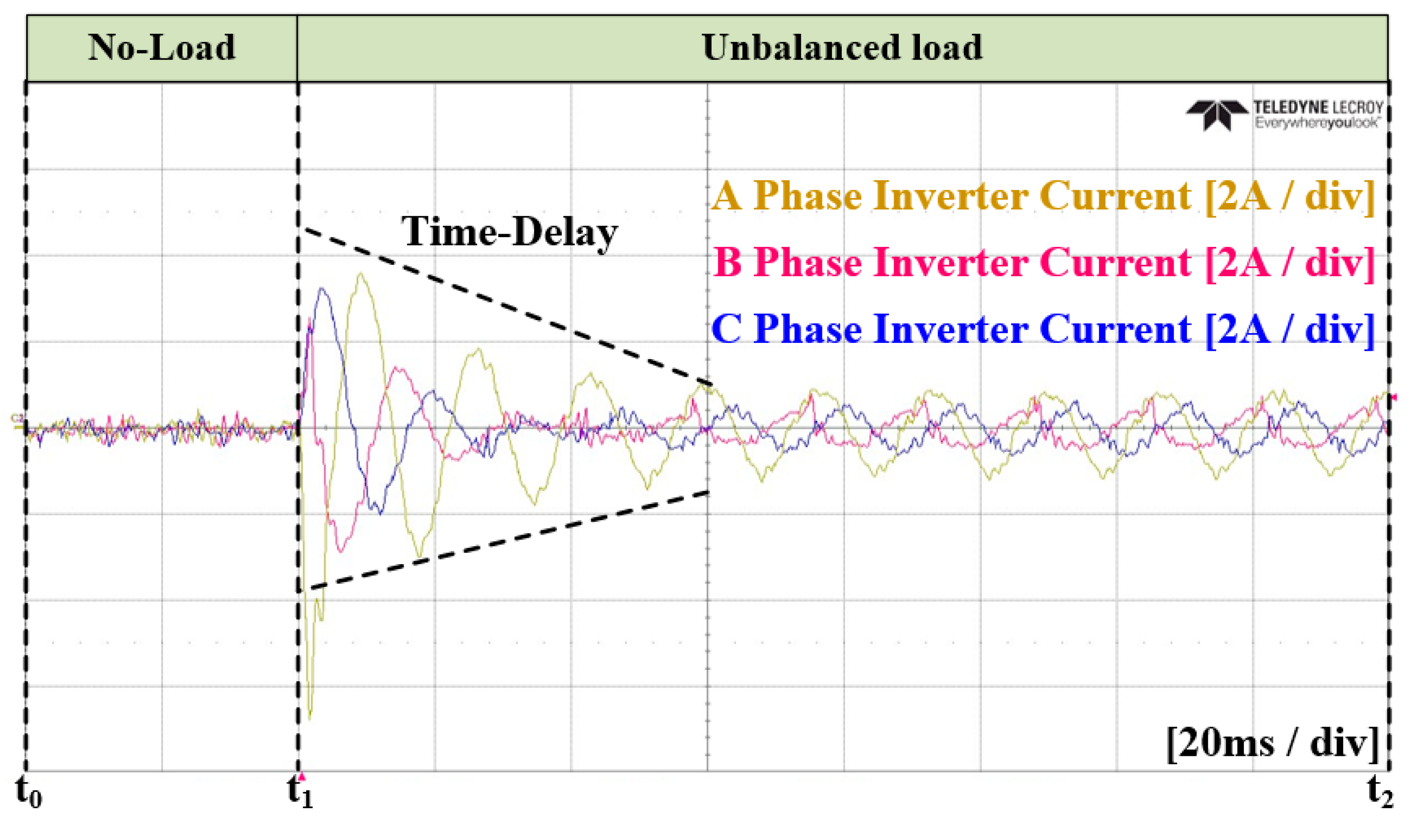
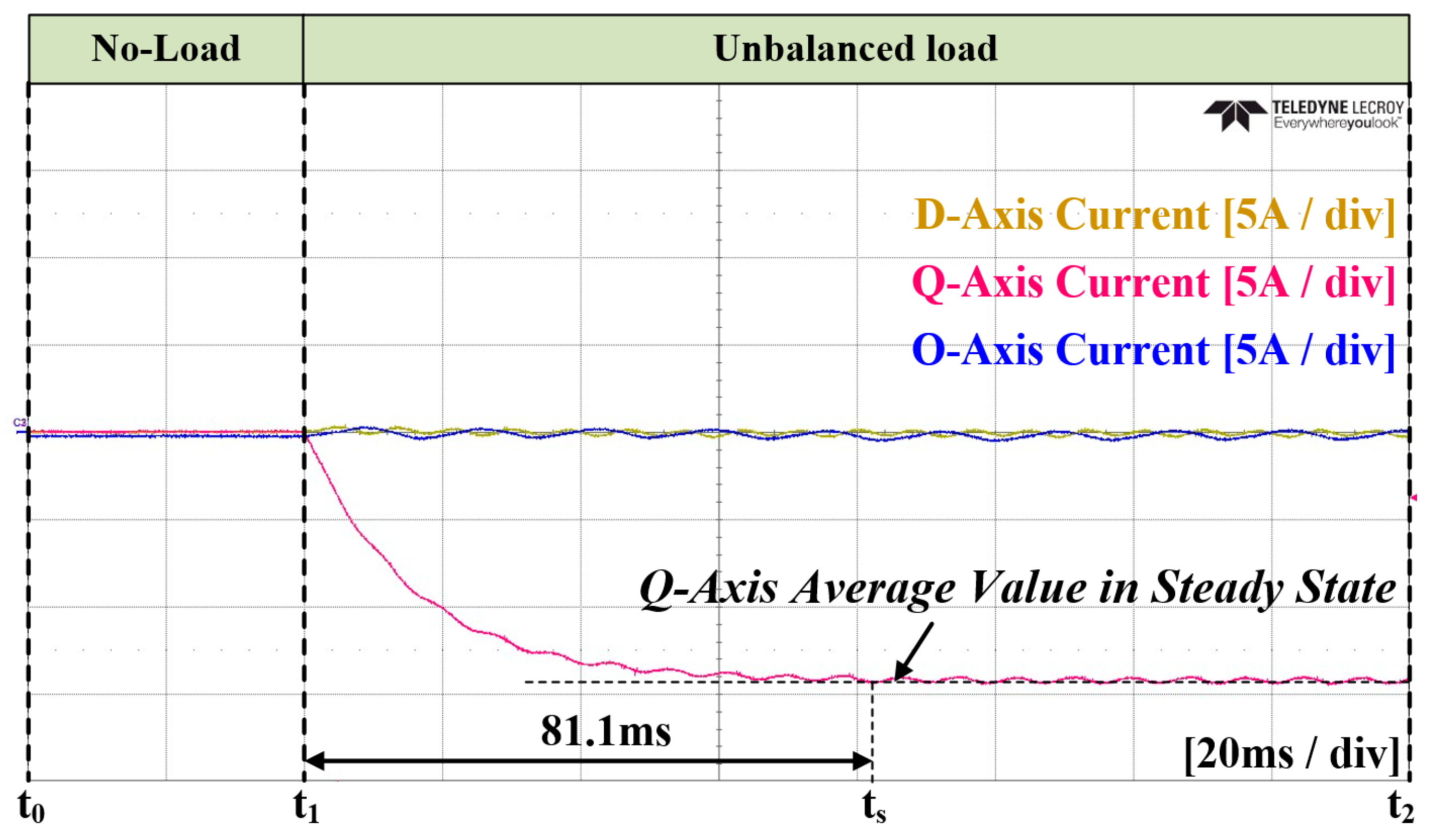
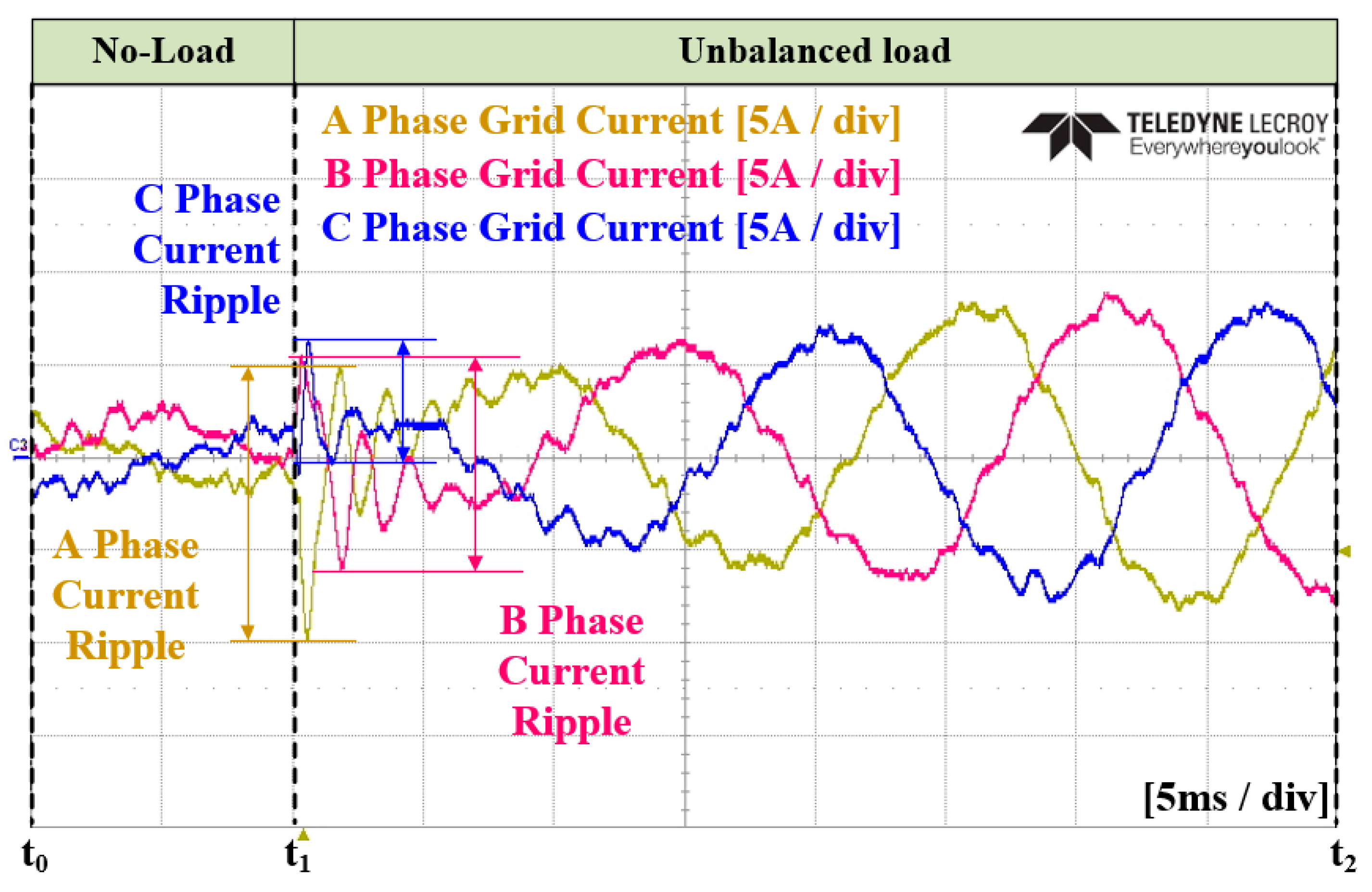
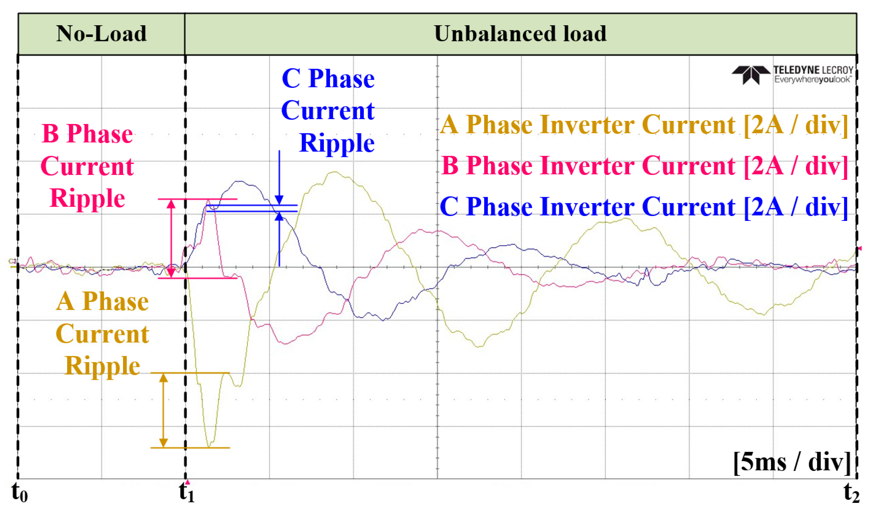
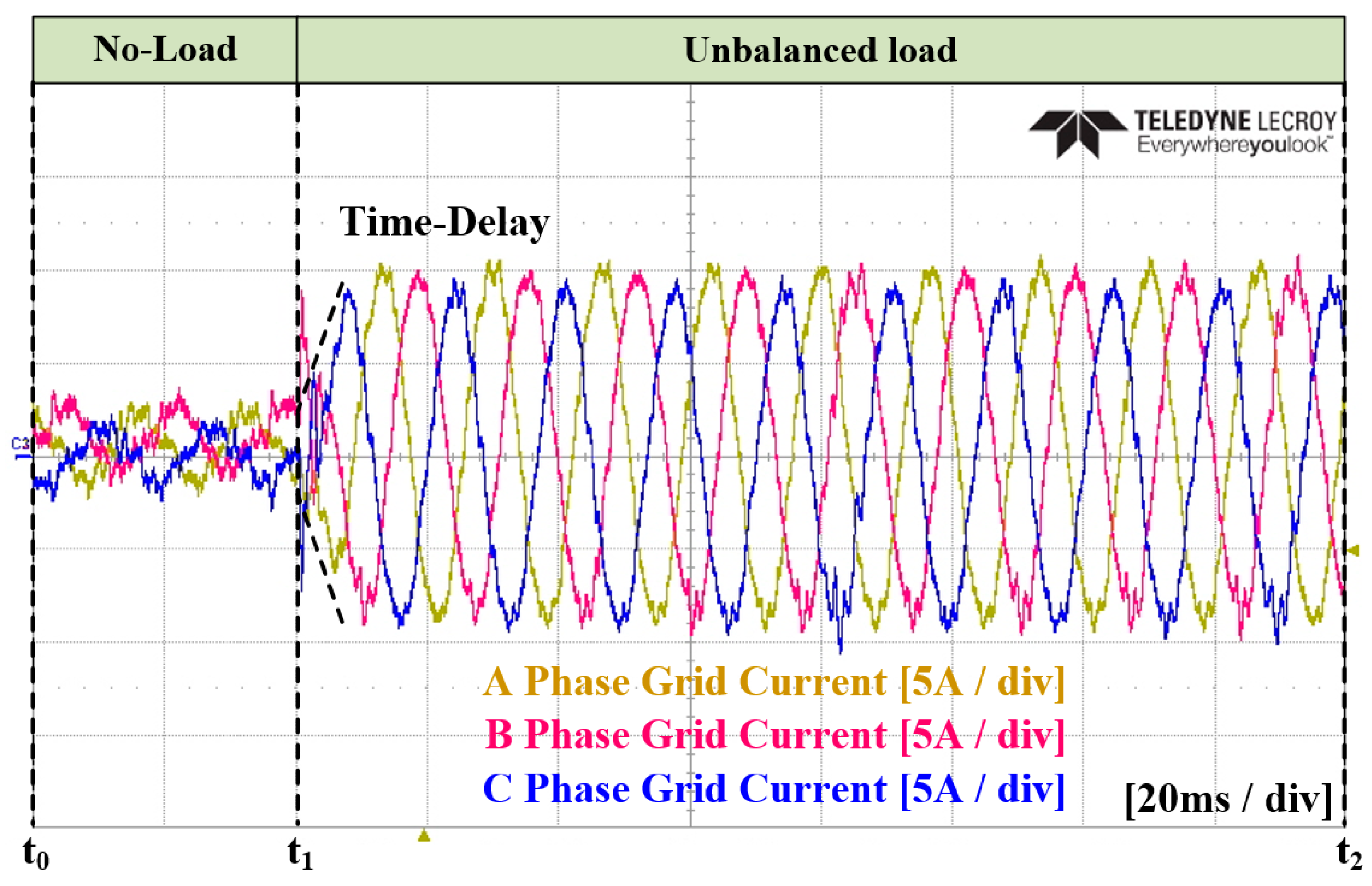
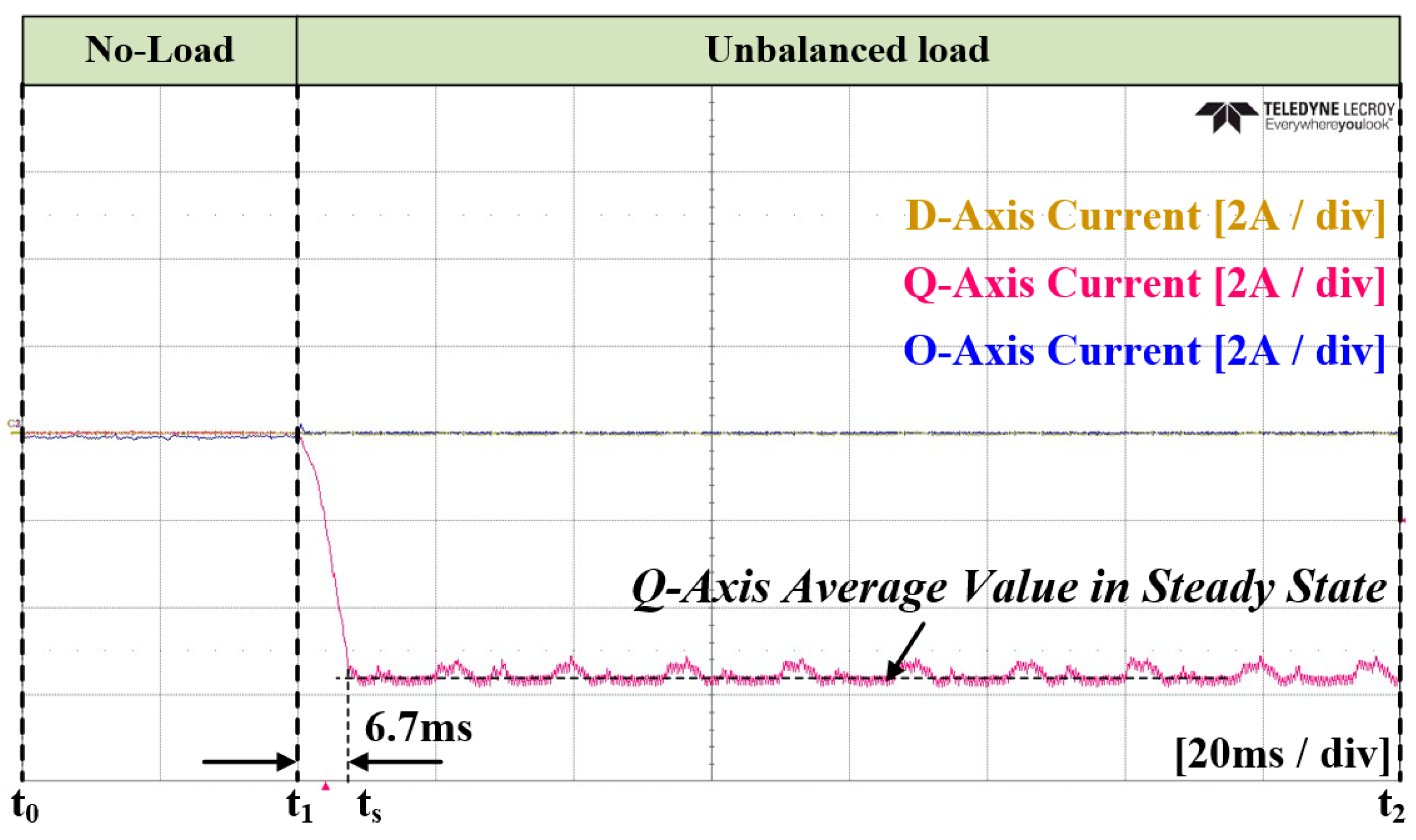
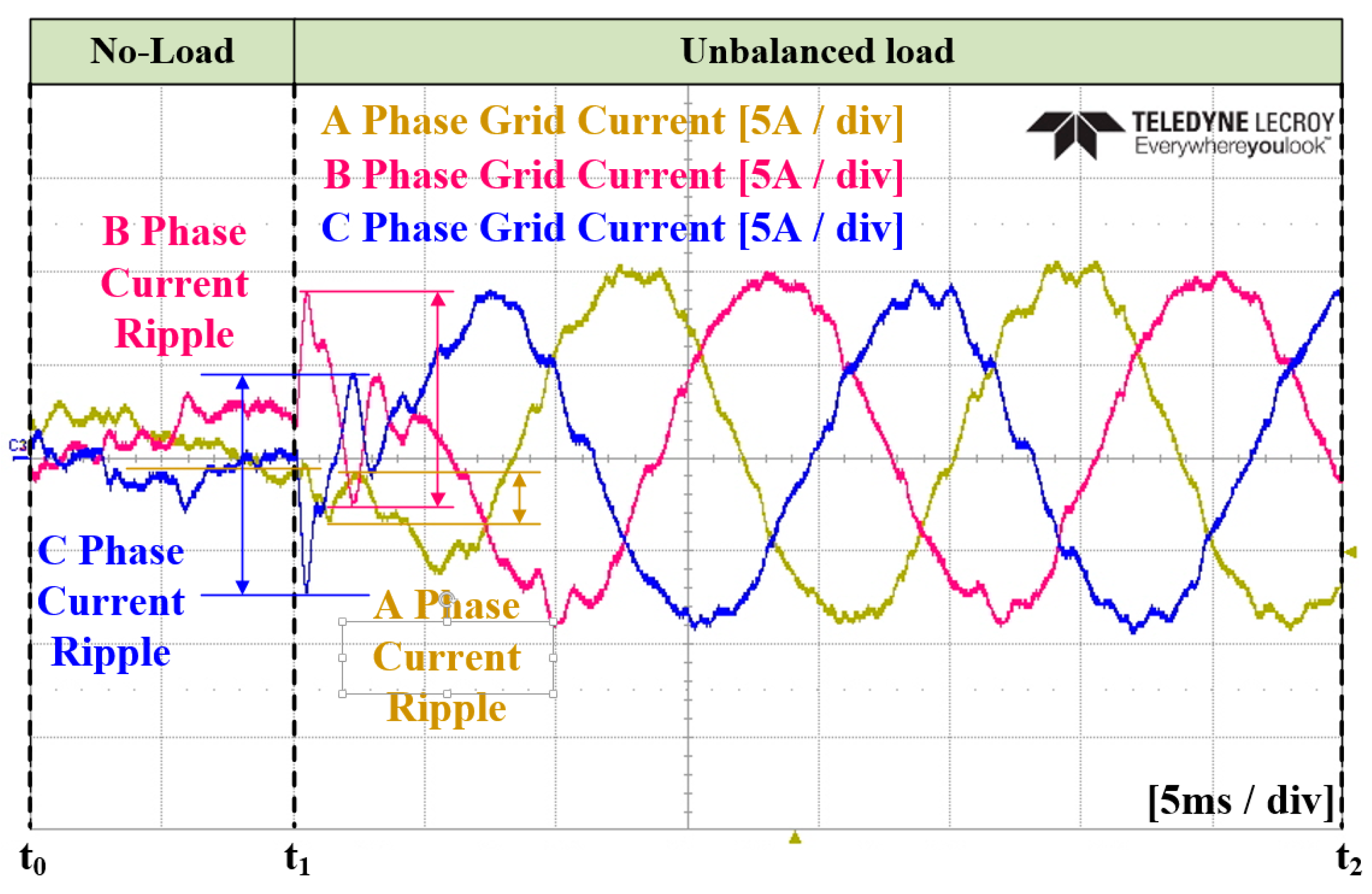
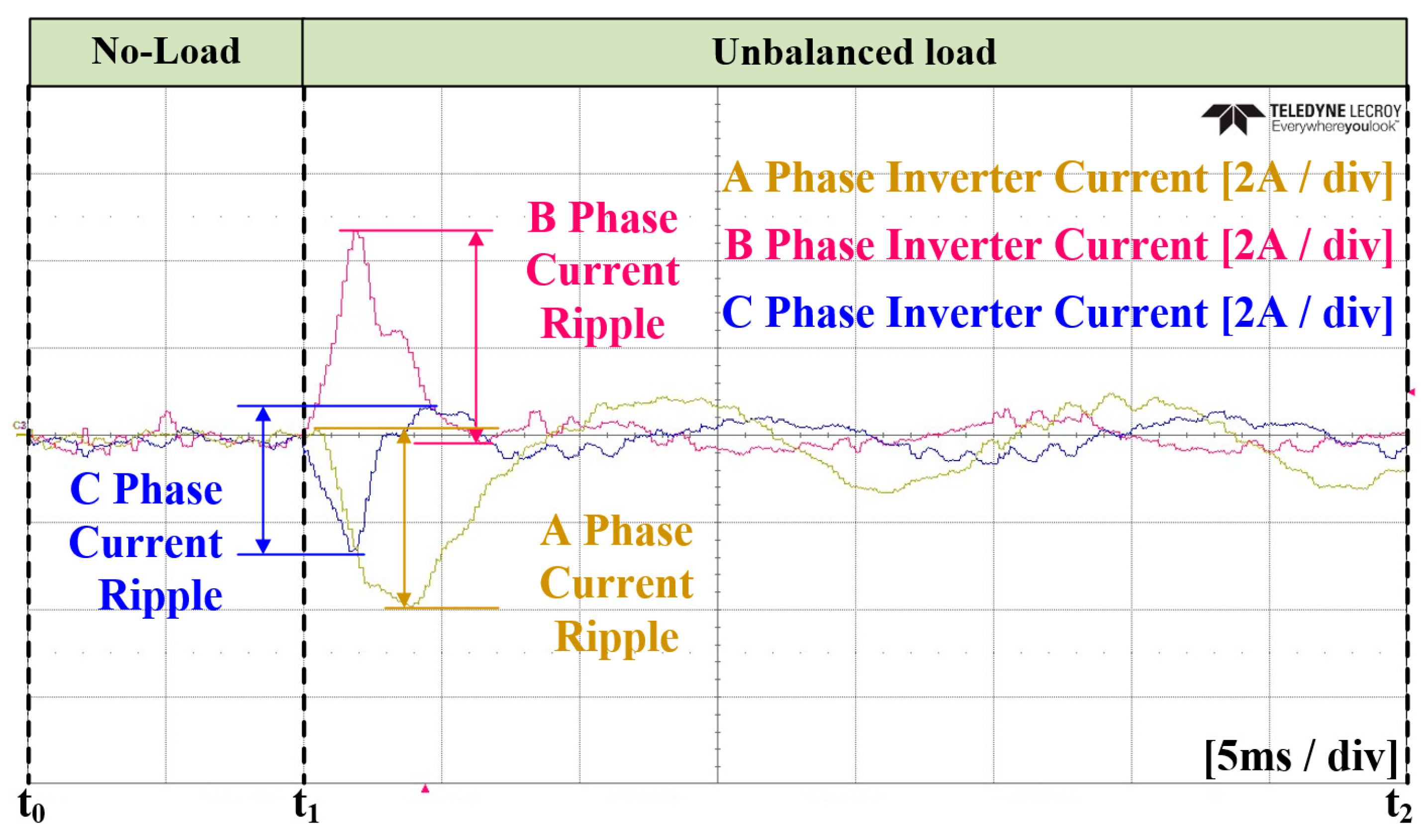
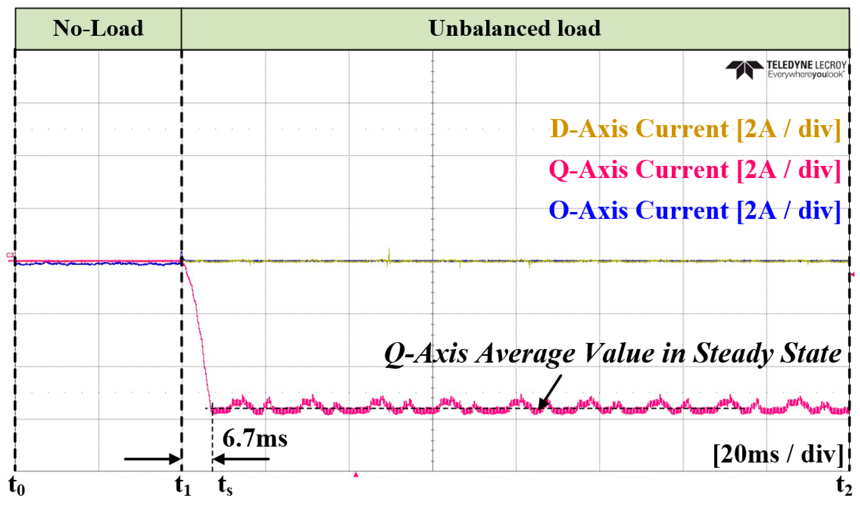
5.1. Case 1 (LPF-Based dq0 Reference Generation and a PI Current Controller)

In the Case 1 experiment, the conventional method was applied. The unbalanced current reference was calculated based on LPF, and a PI current controller was applied. Additionally, the transition to the load state occurred at time $t_1$. Figure 26 and Figure 27, respectively, illustrate the grid current and converter current. Figure 28 represents the amount of unbalance in the dq0 axis using LPF. At time $t_s$, as shown in this figure, it reaches the average value, which takes approximately 81.1 ms. Figure 29 depicts the current reference in the dq0 axis generated by the calculation. Figure 30 and Figure 31 show an enlarged waveform of Figure 26 and Figure 27. The experimental results indicate that it requires more than several cycles to reach the overall steady state.

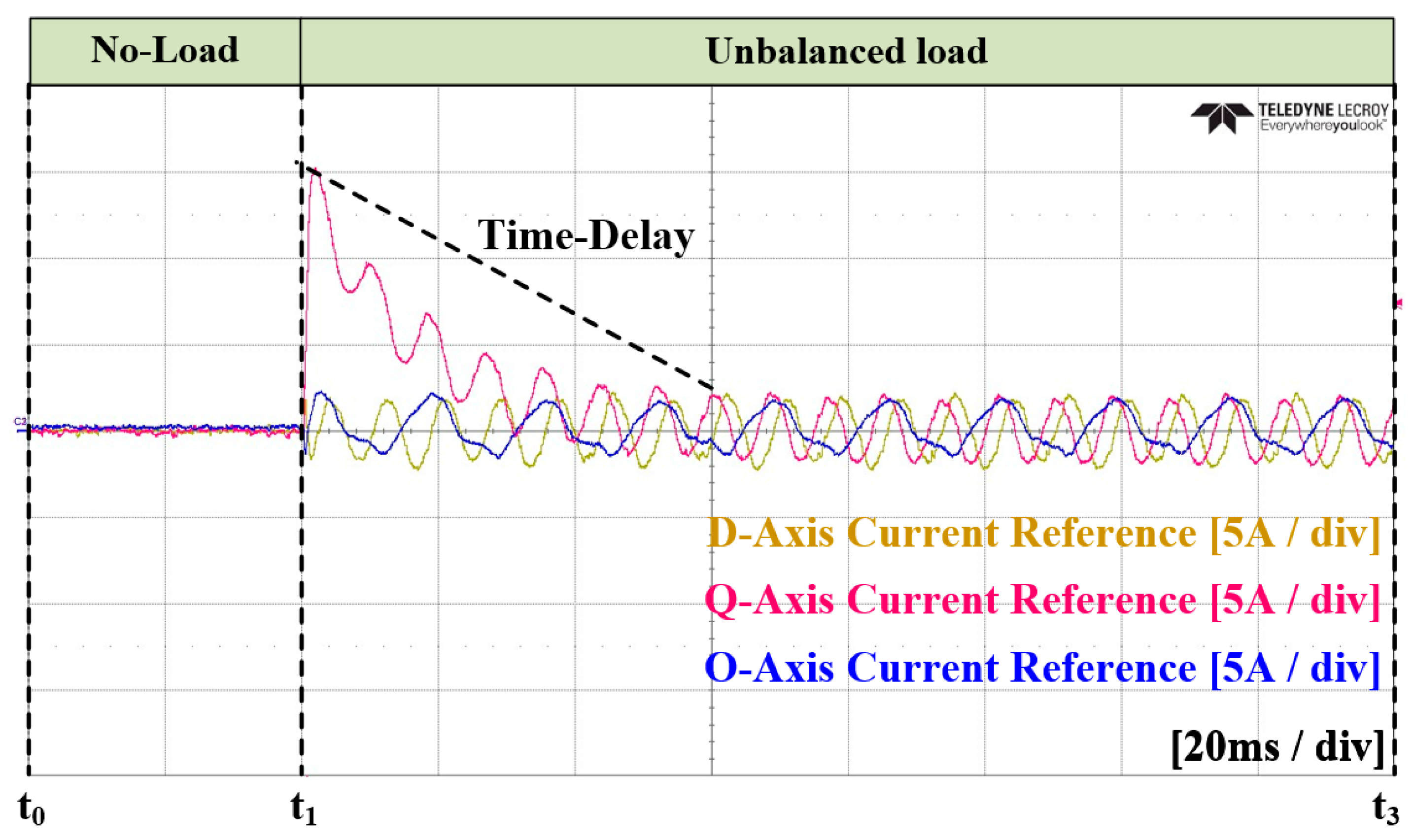
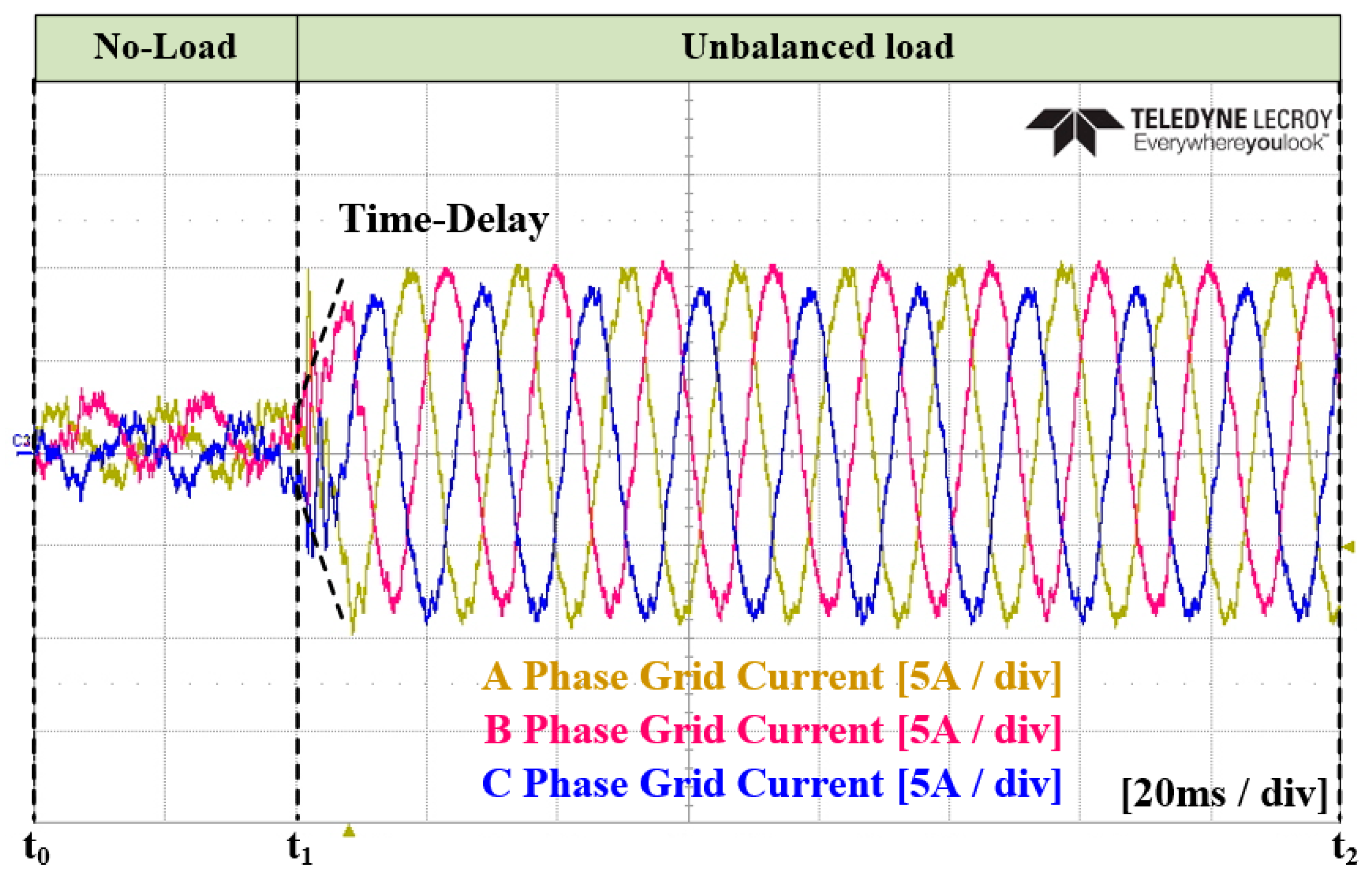
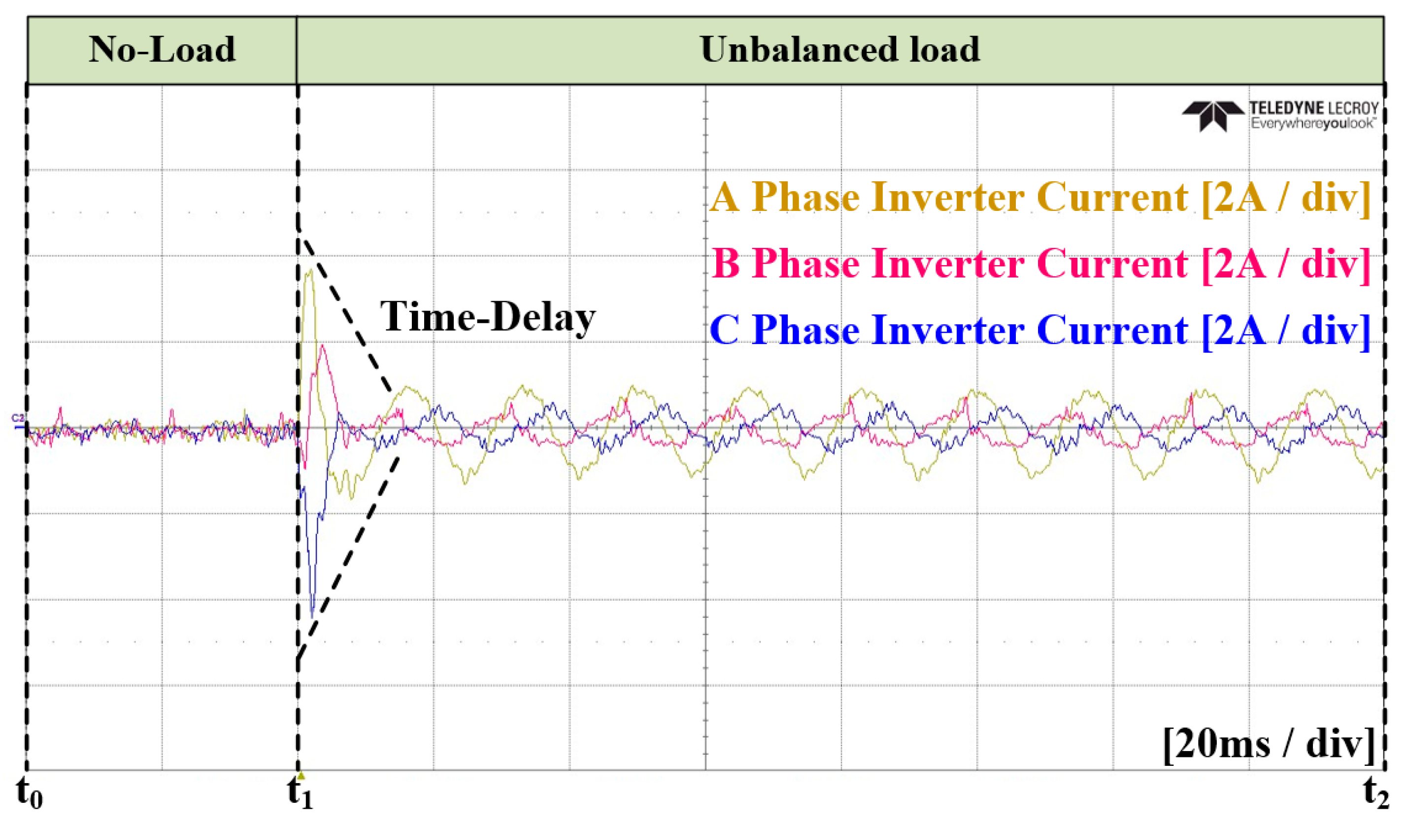
5.2. Case 2 (ANN dq0 Reference Generation and PI Current Controller)

In Case 2 of the experiment, an ANN was applied instead of an LPF for calculating the magnitude of unbalance. The unbalanced current reference was calculated based on the ANN, and a PI current controller was applied. Similar to Case 1, the transition to the load condition occurred at $t_1$. Figure 32 and Figure 33 represent the grid current and the converter current, respectively. Figure 34 illustrates the unbalance in the dq0 axis using an ANN. At $t_s$, it reaches the average value, taking approximately 6.7 ms. Figure 35 depicts the current reference on the dq0 axis calculated by the ANN. Figure 36 and Figure 37 show the zoomed-in waveforms of Figure 32 and Figure 33, respectively. Overall, the experimental results show the achievement of a steady state within one cycle. Additionally, it can be observed that the peak portion of the current exhibits more distortion compared to that noted when the conventional method was applied. However, unlike in the simulations, it appears challenging to quantitatively compare the size of the current ripples due to the inability to transition to the load condition at the same point.

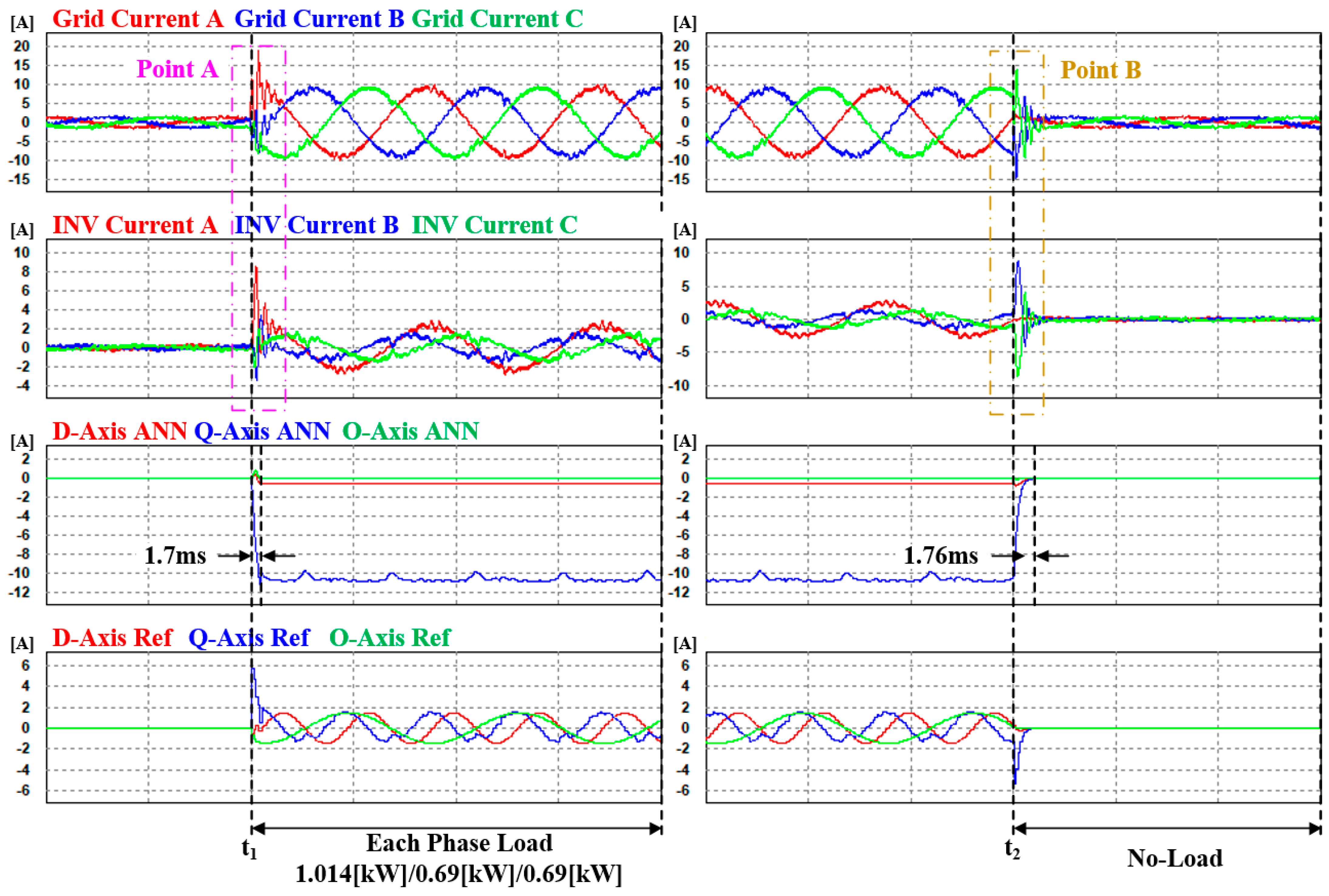
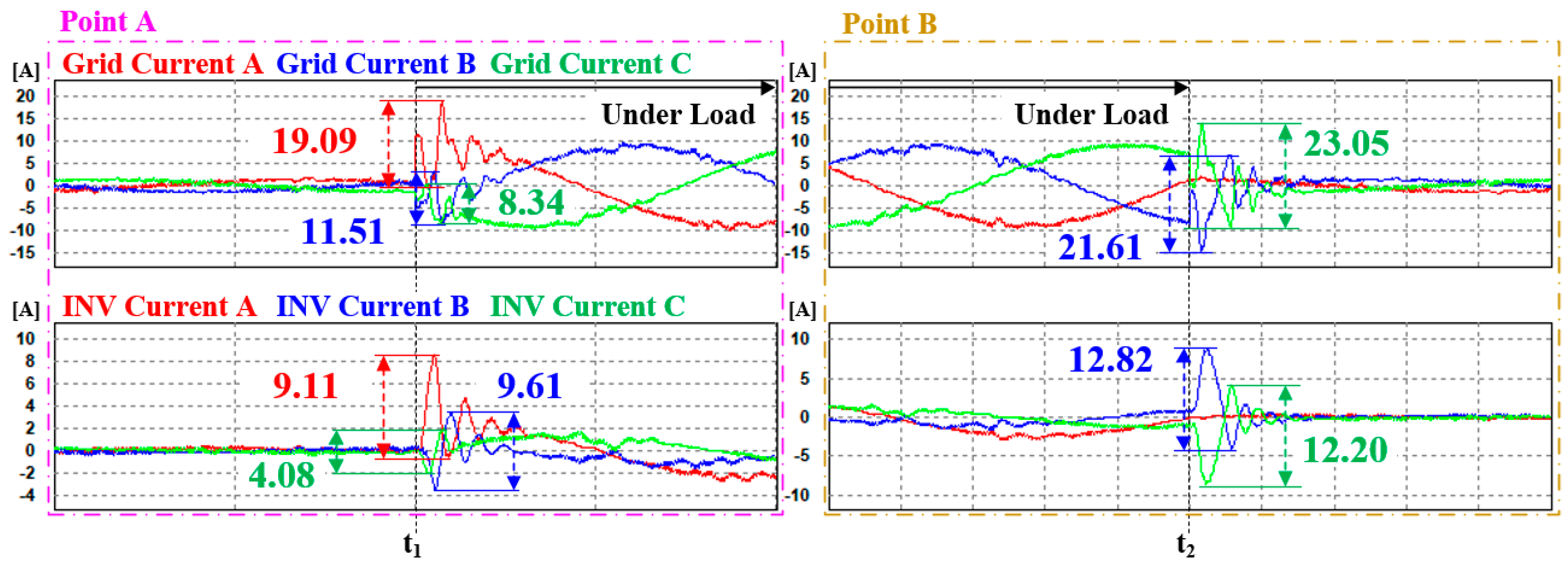
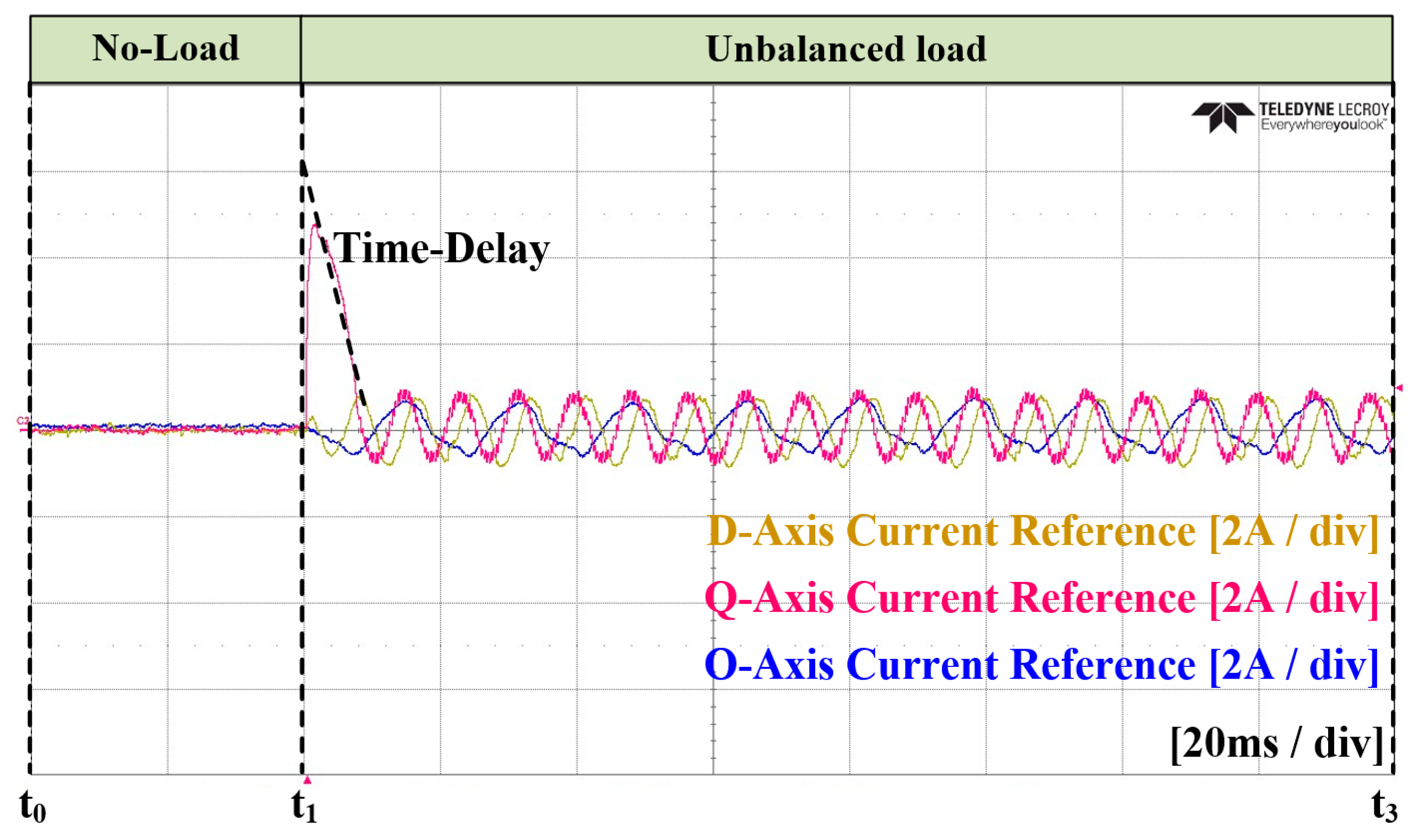
5.3. Case 3 (ANN dq0 Reference Generation and ANN Current Controller)

In the Case 3 experiment, an ANN was applied for unbalanced magnitude calculation and for the current controller. Figure 38 and Figure 39 represent the grid current and converter current, respectively. Figure 40 illustrates the amount of unbalance on the dq0 axis calculated using the ANN. In this figure, it reaches the average value at time $t_s$, which shows a similar time to that noted in Case 2. Figure 41 shows the current reference on the dq0 axis generated by the ANN. Figure 42 and Figure 43 display the enlarged waveforms of Figure 38 and Figure 39, respectively. The experimental results confirm a similar attainment of steady state as that noted in Case 2, with an improvement in distortion at the peak portion of the current.

6. Conclusions

This study aimed to alleviate the current imbalance in power distribution systems with significant load fluctuations in order to obtain balanced power from the power source. The conventional method, which employs an LPF-based dq0 reference generation and a PI current controller, can determine the degree of imbalance, but it requires a low-frequency LPF to extract the magnitude of the AC component. This drawback leads to an excessive time delay. In addition, the PI current controller introduces time delays through the action of the integrator. This poses challenges when applying the method to distribution systems in which loads vary in real-time. To address the aforementioned issues, this study applied an ANN-based reference generator and a current controller to an unbalanced compensation system. The ANN was trained using MATLAB, and the optimal values for the training algorithm and the number of neurons were selected through simulations. To validate the proposed method, simulations and experiments were conducted for the three cases. Case 1 applied the conventional method, Case 2 applied the ANN reference calculation with a PI current controller, and Case 3 applied the ANN reference calculation with an ANN current controller. Case 2 showed a faster estimation of the unbalance compared to Case 1, but it exhibited the drawback of an increased maximum current ripple and a degraded THD. This problem stems from the periodic incorrect output of the ANN reference calculation. In Case 3, by training the ANN current controller with periodic incorrect output and the steady and transient states of the PI controller, the maximum current ripple and THD were improved compared to those noted in Case 1. The improvement in the current THD was confirmed, through simulations and experiments, to be comparable to that of Case 1. Therefore, the proposed ANN-based current compensation method was validated as suitable for power distribution systems with rapidly changing load conditions. In this paper, it was observed that a complete balance of the grid currents could not be achieved due to voltage distortion in the experiments. However, in the future, it will be necessary to research compensation, not only for current, but also for voltage, especially under constrained grid conditions, in order to maintain a higher level of balance.

References

1. Singh, B.; Al-Haddad, K.; Chandra, A. A review of active filters for power quality improvement. IEEE Trans. Ind. Electron. 1999, 46, 960–971. [Google Scholar] [CrossRef]
2. Rafi, F.H.M.; Hossain, M.J.; Rahman, M.S.; Taghizadeh, S. An overview of unbalance compensation techniques using power electronic converters for active distribution systems with renewable generation. Renew. Sustain. Energy Rev. 2020, 125, 109812. [Google Scholar] [CrossRef]
3. Inzunza, R.; Akagi, H. A 6.6-kV transformerless shunt hybrid active filter for installation on a power distribution system. IEEE Trans. Power Electron. 2005, 20, 893–900. [Google Scholar] [CrossRef]
4. Torabi Jafrodi, S.; Ghanbari, M.; Mahmoudian, M.; Najafi, A.; Rodrigues, E.M.G.; Pouresmaeil, E. A Novel Control Strategy to Active Power Filter with Load Voltage Support Considering Current Harmonic Compensation. Appl. Sci. 2020, 10, 1664. [Google Scholar] [CrossRef]
5. Herrera, R.S.; Salmeron, P.; Vazquez, J.R.; Litran, S.P.; Perez, A. Generalized instantaneous reactive power theory in poly-phase power systems. In Proceedings of the 2009 13th European Conference on Power Electronics and Applications, Barcelona, Spain, 8–10 September 2009; pp. 1–10. [Google Scholar]
6. Chen, M.; Jie, Y.; Wang, C.; Li, G.; Qiu, L.; Zhong, W. Optimized Reactive Power Control of Module Power Imbalance of Cascaded Converter. IEEE Open J. Power Electron. 2022, 3, 2–12. [Google Scholar] [CrossRef]
7. Jones, V.; Balda, J.C.; Adapa, R. Current Compensators for Unbalanced Electric Distribution Systems. In Proceedings of the 2018 IEEE Electronic Power Grid (eGrid), Charleston, SC, USA, 12–14 November 2018; pp. 1–6. [Google Scholar] [CrossRef]
8. Vijay, A.S.; Doolla, S.; Chandorkar, M.C. Unbalance mitigation strategies in microgrids. IET Power Electron. 2020, 13, 1687–1710. [Google Scholar] [CrossRef]
9. Hintz, A.; Prasanna, U.R.; Rajashekara, K. Comparative Study of the Three-Phase Grid-Connected Inverter Sharing Unbalanced Three-Phase and/or Single-Phase systems. IEEE Trans. Ind. Appl. 2016, 52, 5156–5164. [Google Scholar] [CrossRef]
10. Siddartha, A.N.R.S.; Basu, T.S.; Chakraborty, C. A simple time domain approach for harmonic, load unbalance and reactive power compensation. In Proceedings of the IECON 2013—39th Annual Conference of the IEEE Industrial Electronics Society, Vienna, Austria, 10–13 November 2013; pp. 8504–8509. [Google Scholar] [CrossRef]
11. Lyu, W.; Wang, R.; Xu, W.; Mu, S.; Guo, R.; Liang, J.; Liu, Z.A. Novel Three Phase Unbalance Detection and Compensation method of Active Power Filter. In Proceedings of the 2018 Chinese Automation Congress (CAC), Xi’an, China, 30 November–2 December 2018; pp. 418–422. [Google Scholar] [CrossRef]
12. Verdelho, P.; Marques, G.D. An active power filter and unbalanced current compensator. IEEE Trans. Ind. Electron. 1997, 44, 321–328. [Google Scholar] [CrossRef]
13. Afonso, J.; Couto, C.; Martins, J. Active Filters with Control based on the p-q Theory. IEEE Ind. Electron. Soc. Newsl. 2000, 47, 5–10. [Google Scholar]
14. Baeckeland, N.; Venkatramanan, D.; Kleemann, M.; Dhople, S. Stationary-Frame Grid-Forming Inverter Control Architectures for Unbalanced Fault-Current Limiting. IEEE Trans. Energy Convers. 2022, 37, 2813–2825. [Google Scholar] [CrossRef]
15. Roiu, D.; Bojoi, R.I.; Limongi, L.R.; Tenconi, A. New Stationary Frame Control Scheme for Three-Phase PWM Rectifiers Under Unbalanced Voltage Dips Conditions. IEEE Trans. Ind. Appl. 2010, 46, 268–277. [Google Scholar] [CrossRef]
16. Somkun, S.; Chunkag, V. Unified Unbalanced Synchronous Reference Frame Current Control for Single-Phase Grid-Connected Voltage-Source Converters. IEEE Trans. Ind. Electron. 2016, 63, 5425–5436. [Google Scholar] [CrossRef]
17. Kesler, M.; Ozdemir, E. Synchronous-Reference-Frame-Based Control Method for UPQC Under Unbalanced and Distorted Load Conditions. IEEE Trans. Ind. Electron. 2011, 58, 3967–3975. [Google Scholar] [CrossRef]
18. Wang, L.; Lam, C.-S.; Wong, M.-C. Unbalanced Control Strategy for A Thyristor-Controlled LC-Coupling Hybrid Active Power Filter in Three-Phase Three-Wire Systems. IEEE Trans. Power Electron. 2017, 32, 1056–1069. [Google Scholar] [CrossRef]
19. Wang, Z.; Wu, B.; Xu, D.; Cheng, M.; Xu, L. DC-Link Current Ripple Mitigation for Current-Source Grid-Connected Converters Under Unbalanced Grid Conditions. IEEE Trans. Ind. Electron. 2016, 63, 4967–4977. [Google Scholar] [CrossRef]
20. Herrera, R.S.; Salmerón, P.; Kim, H. Instantaneous Reactive Power Theory Applied to Active Power Filter Compensation: Different Approaches, Assessment, and Experimental Results. IEEE Trans. Ind. Electron. 2008, 55, 184–196. [Google Scholar] [CrossRef]
21. Bhattacharya, A.; Chakraborty, C.; Bhattacharya, S. Shunt compensation. IEEE Ind. Electron. Mag. 2009, 3, 38–49. [Google Scholar] [CrossRef]
22. Sun, Y.; Li, S.; Fu, X.; Dong, W.; Ramezani, M.; Balasubramanian, B. Approximate dynamic programming vector controllers for operation of IPM motors in linear and overmodulation regions. IEEE Trans. Transp. Electrif. 2020, 7, 659–670. [Google Scholar] [CrossRef]
23. Dong, W.; Li, S.; Fu, X.; Li, Z.; Fairbank, M.; Gao, Y. Control of a buck DC/DC converter using approximate dynamic programming and artificial neural networks. IEEE Trans. Circuits Syst. I Regul. Pap. 2021, 68, 1760–1768. [Google Scholar] [CrossRef]
24. Gupta, N.; Singh, S.P.; Dubey, S.P. Neural network based shunt active filter for harmonic and reactive power compensation under non-ideal mains voltage. In Proceedings of the 5th IEEE Conference on Industrial Electronics and Applications, Taichung, Taiwan, 15–17 June 2010. [Google Scholar]
25. Fang, Z.P.; Lai, J.-S. Generalized instantaneous reactive power theory for three-phase power systems. IEEE Trans. Instrum. Meas. 1996, 45, 293–297. [Google Scholar] [CrossRef]
26. George, J.; Jose, T.L.; Jacob, J. A decoupled reference generation algorithm for harmonic, reactive power and current unbalance compensation in three-phase systems. In Proceedings of the 2011 Annual IEEE India Conference, Hyderabad, India, 16–18 December 2011; pp. 1–6. [Google Scholar] [CrossRef]
27. Kim, G.-H.; Hwang, C.; Jeon, J.-H.; Ahn, J.-B.; Kim, E.S. A novel three-phase four-leg inverter based load unbalance compensator for stand-alone microgrid. Int. J. Electr. Power Energy Syst. 2015, 65, 70–75. [Google Scholar] [CrossRef]
28. Kim, S.-H. An Energy Management Method Using ANN and Hierarchical Control for Bipolar DC Microgrid Based on Droop Control. Ph.D. Thesis, Sungkyunkwan University Graduate School, Seoul, Republic of Korea, 2023. [Google Scholar]
Figure 1. Unbalanced current compensation configuration.
Energies 17 01325 g001
Figure 2. Unbalanced load current compensation vector diagram.
Energies 17 01325 g002
Figure 3. Current reference calculation based on the instantaneous p-q theory [13].
Energies 17 01325 g003
Figure 4. Current reference calculation based on the synchronous reference frame method [27].
Energies 17 01325 g004
Figure 5. Proposed current compensating method control block diagram based on ANN.
Energies 17 01325 g005
Figure 6. The structure of the ANN applied in this paper.
Energies 17 01325 g006
Figure 7. Example of the activation function.
Energies 17 01325 g007
Figure 8. ANN structure in MATLAB.
Energies 17 01325 g008
Figure 9. MSE of ANN training according to dataset ratio.
Energies 17 01325 g009
Figure 10. ANN training results according to the algorithm.
Energies 17 01325 g010aEnergies 17 01325 g010b
Figure 11. ANN training results based on the number of hidden neurons.
Energies 17 01325 g011aEnergies 17 01325 g011b
Figure 12. ANN configuration of current reference calculation.
Energies 17 01325 g012
Figure 13. Training result of ANN for current reference calculation.
Energies 17 01325 g013
Figure 14. ANN configuration of dq0 axis.
Energies 17 01325 g014
Figure 15. Training results for an ANN for the current controller of dq0 axis.
Energies 17 01325 g015aEnergies 17 01325 g015b
Figure 16. Simulation and experimental setup configuration.
Energies 17 01325 g016
Figure 17. Nominal voltage and current under unbalanced load conditions.
Energies 17 01325 g017
Figure 18. Case 1 simulation of waveforms with LPF-based dq0 reference generation and a PI current controller.
Energies 17 01325 g018
Figure 19. Enlarged transient state waveforms of each point with LPF-based dq0 reference generation and a PI current controller.
Energies 17 01325 g019
Figure 20. Case 2 simulation waveforms, with ANN dq0 reference generation and a PI current controller.
Energies 17 01325 g020
Figure 21. Enlarged transient state waveforms of each point, with ANN dq0 reference generation and a PI current controller.
Energies 17 01325 g021
Figure 22. Case 3 simulation waveforms, with ANN dq0 reference generation and ANN current controller.
Energies 17 01325 g022
Figure 23. Enlarged transient state waveforms of each point, with ANN dq0 reference generation and ANN current controller.
Energies 17 01325 g023
Figure 24. Experimental configuration of current compensation under the unbalanced load conditions.
Energies 17 01325 g024
Figure 25. Nominal voltage and current under unbalanced load conditions in the experiment.
Energies 17 01325 g025
Figure 26. Experimental waveforms of the three-phase grid current in Case 1.
Energies 17 01325 g026
Figure 27. Experimental waveforms of the three-phase inverter current in Case 1.
Energies 17 01325 g027
Figure 28. Experimental waveforms of the filtered dq0 value in Case 1.
Energies 17 01325 g028
Figure 29. Experimental waveforms of the dq0 current reference in Case 1.
Energies 17 01325 g029
Figure 30. Enlarged waveform of the three-phase grid current in Case 1.
Energies 17 01325 g030
Figure 31. Enlarged waveform of the three-phase inverter current in Case 1.
Energies 17 01325 g031
Figure 32. Experimental waveforms of the three-phase grid current in Case 2.
Energies 17 01325 g032
Figure 33. Experimental waveforms of the three-phase inverter current in Case 2.
Energies 17 01325 g033
Figure 34. Experimental waveforms of the ANN output value in Case 2.
Energies 17 01325 g034
Figure 35. Experimental waveforms of the dq0 current reference in Case 2.
Energies 17 01325 g035
Figure 36. Enlarged waveform of the three-phase grid current in Case 2.
Energies 17 01325 g036
Figure 37. Enlarged waveform of the three-phase inverter current in Case 2.
Energies 17 01325 g037
Figure 38. Experimental waveforms of the three-phase grid current in Case 3.
Energies 17 01325 g038
Figure 39. Experimental waveforms of the three-phase inverter current in Case 3.
Energies 17 01325 g039
Figure 40. Experimental waveforms of the ANN output value in Case 3.
Energies 17 01325 g040
Figure 41. Experimental waveforms of the dq0 current reference in Case 3.
Energies 17 01325 g041
Figure 42. Enlarged waveform of the three-phase grid current in Case 3.
Energies 17 01325 g042
Figure 43. Enlarged waveform of the three-phase inverter current in Case 3.
Energies 17 01325 g043