Abstract
The prognosis of wind turbine failures in real operating conditions is a significant gap in the academic literature and is essential for achieving viable performance parameters for the operation and maintenance of these machines, especially those located offshore. This paper presents a framework for estimating the remaining useful life (RUL) of the main bearing using regression models fed operational data (temperature, wind speed, and the active power of the network) collected by a supervisory control and data acquisition (SCADA) system. The framework begins with a careful data filtering process, followed by creating a degradation profile based on identifying the behavior of temperature time series. It also uses a cross-validation strategy to mitigate data scarcity and increase model robustness by combining subsets of data from different available turbines. Support vector, gradient boosting, random forest, and extra trees models were created, which, in the tests, showed an average of 20 days in estimating the remaining useful life and presented mean absolute error (MAE) values of 0.047 and mean squared errors (MSE) of 0.012. As its main contributions, this work proposes (i) a robust and effective regression modeling method for estimating RUL based on temperature and (ii) an approach for dealing with a lack of data, a common problem in wind turbine operation. The results demonstrate the potential of using these forecasts to support the decision making of the teams responsible for operating and maintaining wind farms.
1. Introduction
Since the beginning of the 21st century, the pursuit of developing and enhancing renewable energy production has been driven by environmental regulations, new business prospects, and a shifting global mindset regarding the significance of utilizing energy sources with minimal impact on the planet [1].
In this context, wind energy, a resource harnessed by humans for centuries, currently stands out for its advanced technological level and widespread use in various countries, both onshore and offshore. In terms of design, modern wind turbines surpass 120 m hub heights, 200 m rotor diameters, and 5 MW production capacity barriers. Operationally, wind farms have expanded in size, increasingly venturing into waters far from the coast and employing specialized monitoring and control systems to ensure safety and efficiency throughout their life cycle.
However, these large machines entail high operating and maintenance costs, around 12% for onshore installations and up to 23% [2] for offshore installations. The companies operating and maintaining them have been striving to employ more precise and effective maintenance methods and techniques to achieve more profitable production levels [3] and enhanced safety.
In the wind energy industry, particularly offshore, corrective maintenance is undesirable due to its high costs and operational and environmental impacts. Therefore, preventive and predictive maintenance are utilized to avoid early wind turbine failures. Predictive maintenance, a technique based on condition monitoring as per NSAI [4], is carried out using forecasts from the repeated analysis or evaluation of parameters and characteristics indicating component degradation. This type of maintenance necessitates investment in sensors, equipment to collect data from critical machine components, and human capital capable of interpreting the data to generate relevant information for the decision making of senior managers.
Vibration monitoring is an effective predictive technique for identifying component degradation in mechanical assemblies. However, in applications such as wind turbines, where there is a wide range of load variation, randomly, over short periods [5] (pp. 178–227), and in low-speed conditions, it is a challenge to identify incipient faults in bearings and gears. In these cases, it is necessary to identify and analyze changes in the vibrational signature of these components concerning the start of operation or its replacement.
Temperature monitoring also provides valuable data. Analyzing deviations in historically observed temperature values can reveal possible flaws in development, allowing for early corrections before major problems occur.
In order to successfully implement condition-based maintenance (CBM), sophisticated techniques for fault detection, diagnosis, and prediction that satisfy the wind energy sector’s technical, operational, safety, and environmental requirements must be used.
Consequently, to carry out a failure prognosis, the earlier it is possible to identify a degradation profile in which the data show a monotonic signal with a trend, the more successful the prognosis estimation will be.
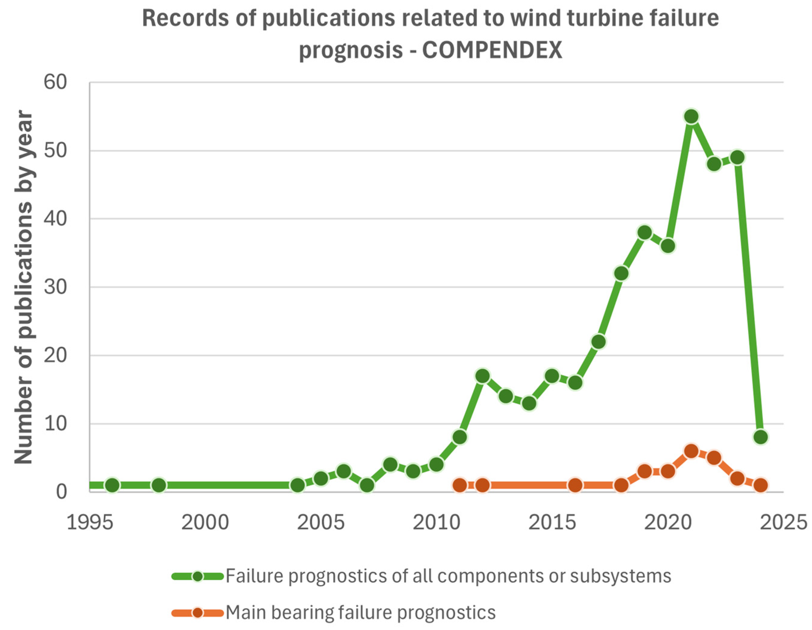
Fault prognosis is the next frontier that the wind energy industry seeks. From this perspective, there has been an explosion of articles since 2014 investigating the use of data-driven methods and models for the assessment of remaining useful life (RUL), as shown in Figure 1, addressing different failure prognosis techniques in the kinematic assembly, mainly in wind turbine speed reducers. Several authors [6,7,8,9,10] have used machine learning techniques or artificial neural networks (ANN) to estimate the RUL of gears and bearings in speed reducers and carry out failure prognoses. Still, the number of studies for main bearing prognosis is significantly lower [2,11], as shown in Figure 1.
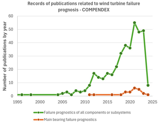
Figure 1.
Number of records of publications related to failure prognostics of all components or subsystems and failure prognostics of main bearing of wind turbines on Engineering Village (COMPENDEX).
Some studies [12,13] employing hybrid models with deep neural networks have focused on main bearing fatigue estimates. Other studies advance the estimation of the RUL of the main bearing using natural neural network models (e.g., LSTM) [9]. The authors emphasize the need for data manipulation, data augmentation [13], and resampling [9] to estimate fatigue or RUL.
Challenges in the failure prognosis of wind turbine main bearings stem from the lack of understanding of the relationship between load and damage and frequency and failure modes in real applications [11].
An accurate calculation of the RUL estimate is crucial for cost-effective maintenance and greater wind turbine availability. Machine learning and artificial intelligence algorithms enable the utilization of a massive amount of data from the condition-based maintenance system and the supervision and data acquisition system to estimate the RUL of power train components [7,14].
The use of variables like temperature is proposed as an alternative for identifying faults and conducting prognosis. Wind turbine supervisory control systems (SCADA) monitor the temperatures of the various components of the kinematic assembly, from the main bearing to the bearing on the opposite side of the coupling and of the Nacelle and the environment. It is possible to set temperature limits based on technical information about the components and lubricants used.
This article presents a methodology for estimating the RUL of main bearings from regression models using real wind turbine data. The models were built with the a priori definition of an RUL profile through the analysis of local temperature time series, creation of training sets, validation and testing with different turbine time series, evaluation of metrics such as mean squared error (MSE), root mean squared error (RMSE), mean absolute error (MAE), and the coefficient of determination (R2 Score), and estimation of RUL using the test dataset.
The main contributions of this article include the following:
- The development of a robust framework for estimating RUL from real main bearing temperature series from a SCADA system;
- The presentation of a cross-validation strategy to mitigate the issue of scarce data and increase models’ generalization capacities.
2. Methodology for Wind Turbine Useful Life Estimation
This paper presents a framework for predicting wind turbine failures by estimating the remaining useful life of the main bearing using temperature data monitored by a SCADA system. The framework used raw main bearing temperature data and regression models to calculate the RUL of turbines from two wind farms installed on the coast of northeastern Brazil. The turbines were all the same model and had a rated power above 1 MW. Detailed information cannot be made available for confidentiality reasons.
The procedure consists of reading and preprocessing the raw data from the SCADA system and creating a degradation profile based on the temperature behavior with the design limits. The main bearing average temperature, environment average temperature, wind speed, and active grid power data within the operational range of the wind turbines were considered variables of interest. The environmental conditions and mechanical properties of the main bearing lubricant of three wind turbines with different degradation dynamics were also accounted for. Simulation cases were then defined from the datasets of these three turbines, respectively, for training, validating, and testing machine learning models using regression models.
The MSE, RMSE, MAE, and R2 Score metrics were calculated for the regression models developed, and rankings were made based first on the MAE and then on the R2 Score. The two models with the lowest MAEs and highest R2 Scores were chosen to estimate the RUL of the wind farm’s main turbine bearing.
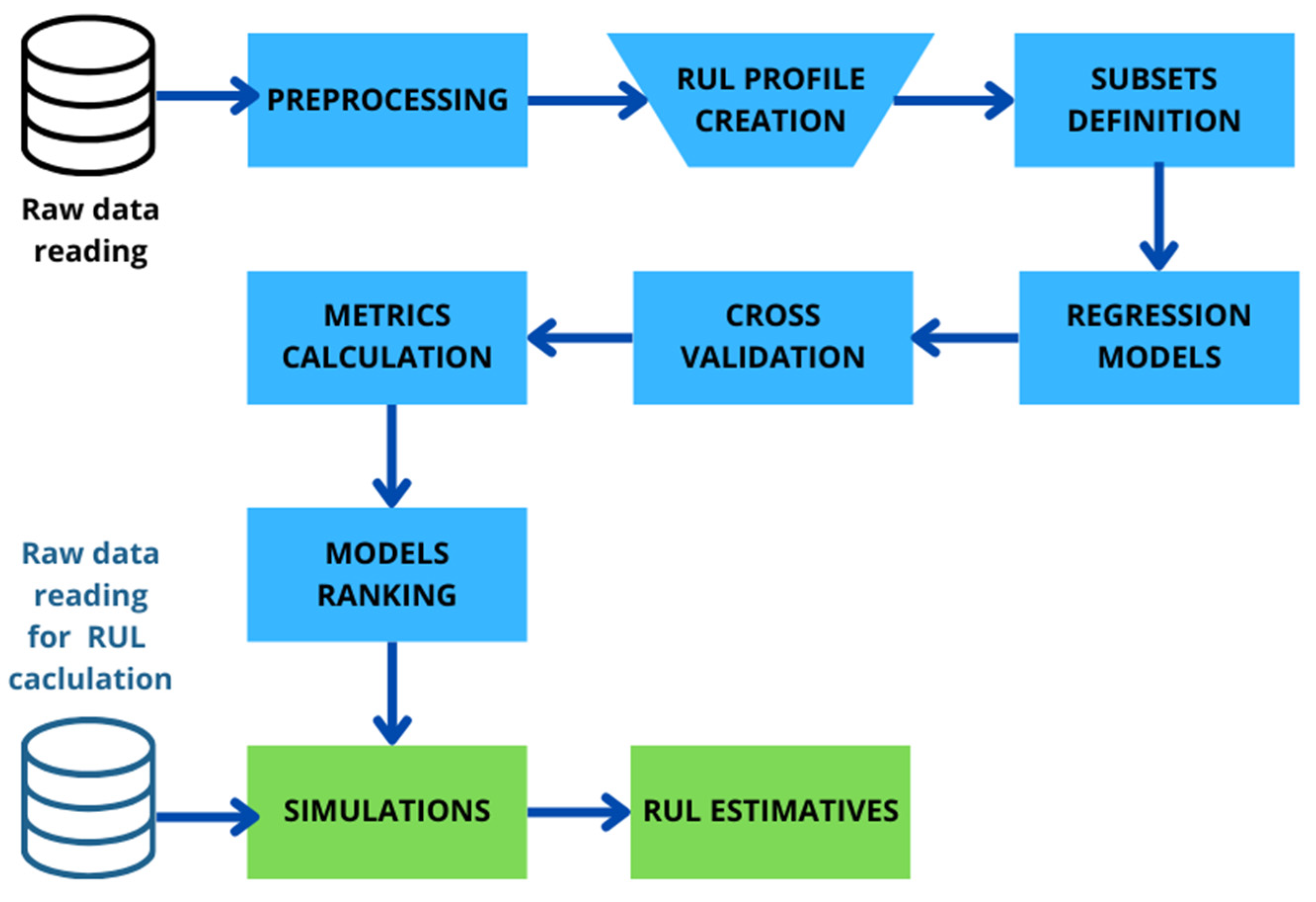
Figure 2 shows the flowchart for estimating the RUL of the main bearing from temperature data.

Figure 2.
RUL estimation using regression machine learning models.
As shown in Figure 2, the overall method consists of eleven stages. In the first stage, the raw data from the SCADA system is read. The second stage aims for the preprocessing stage of the data with cleaning, filtering, and resampling techniques. The third stage aims for data classification. The fourth stage involves the creation of data for training, validation, and testing, and the available data are separated into subsets. The fifth stage aims to prepare and train the regression models. In the sixth stage, cross-validation is carried out to identify the best hyperparameters of the models. The seventh stage is linked to the determination of the study metrics. In the eighth stage, the models are ranked, and the best ones are selected. The simulations are carried out to estimate the remaining useful life (RUL) based on reading data from the test subsets in the ninth stage. In the tenth stage, the simulation with the best regressive models is carried out, and finally, in the eleventh stage, the RUL is calculated.
2.1. SCADA System Data Reading and Preprocessing
The SCADA system has a lower data acquisition rate than condition-based maintenance systems [15] (pp. 303–342). The signals are recorded in 10 min samples over a given time interval, but they can still identify faults generated by components and subsystems that involve changes in measured quantities. The raw turbine data from the two wind farms were provided in “.csv” format and were read and condensed into a parquet file. A single data frame was created containing all the SCADA variables with the data from the parquet file, which we will call the raw data dataset. From the raw data dataset, a new one was created with only the time series with the variables of interest (main bearing average temperature, environment average temperature, windspeed average status, grid average active power) of 34 wind turbines (WT1–WT34) from the two wind farms.
Figure 3 shows the preprocessing of the signal. In the first step, the data were filtered to remove measurements where the wind speed was greater than or equal to 3.5 m/s, generator speed was below 1198 RPM or above 1200 RPM, and ambient temperature was less than or equal to 50 degrees Celsius, which were outside the turbine’s operating conditions. The temperature series was then resampled at 1 h intervals to filter out intra-hour variations. In the second step, a feature was created by subtracting the ambient temperature from the main bearing temperature value as outlined by Wiese et al. [16], which we will call temperature variation, to remove the influence of the ambient temperature on the main bearing behavior.

Figure 3.
Signal preprocessing.
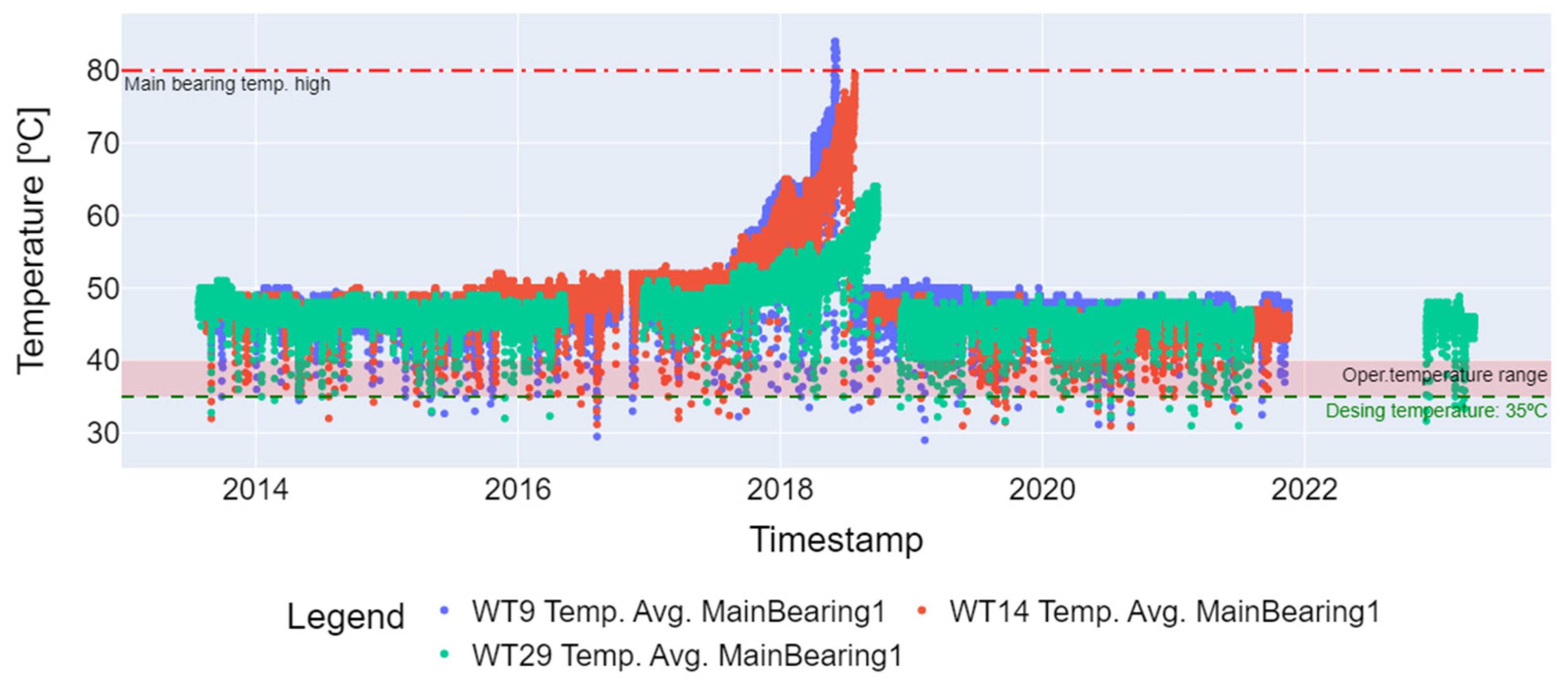
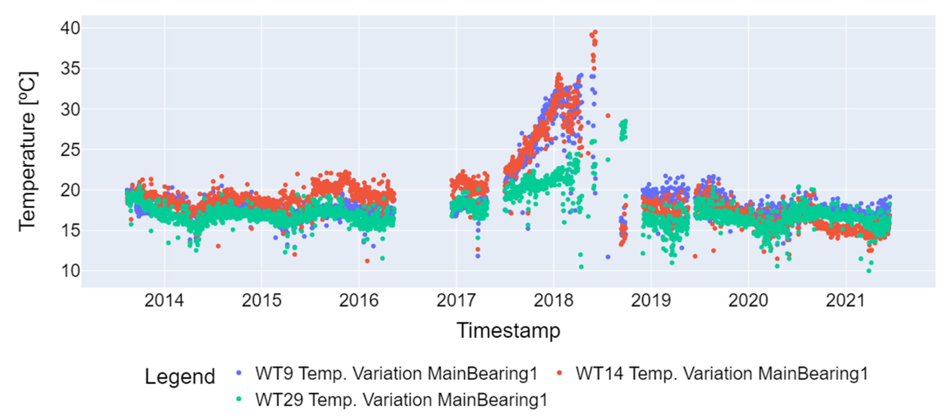
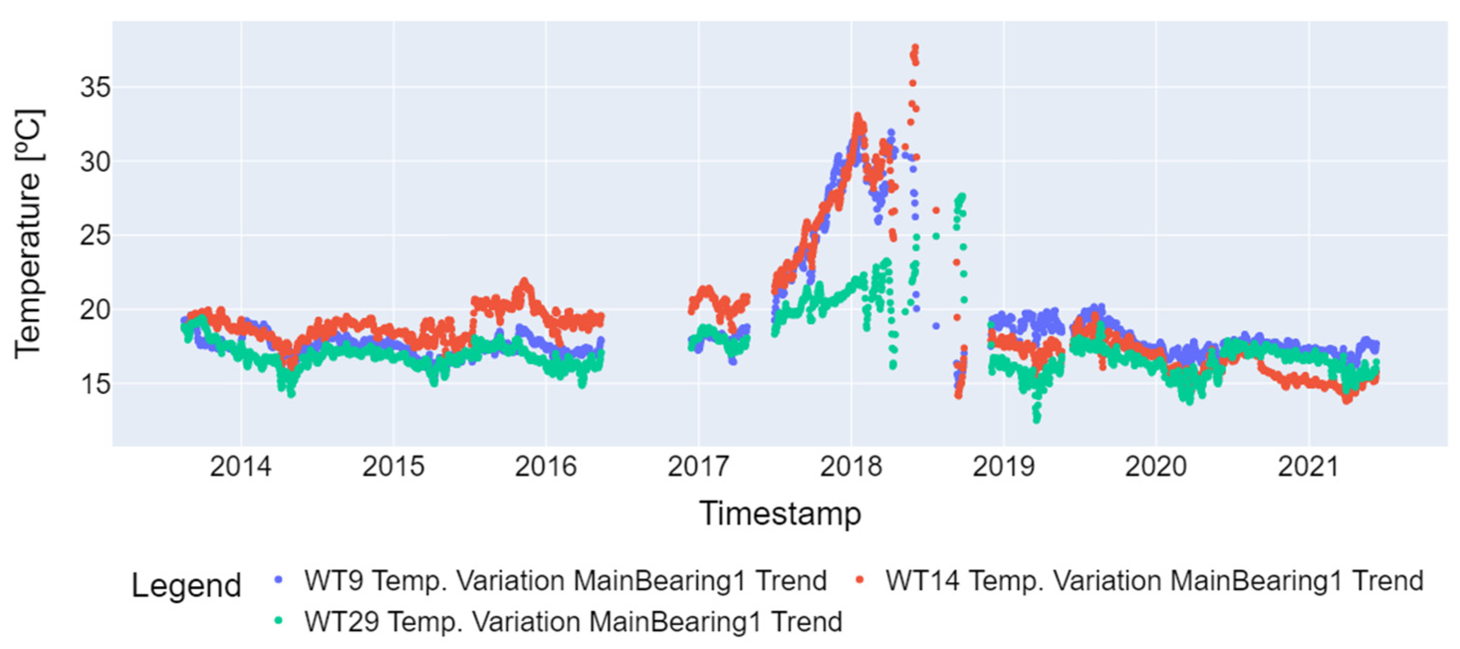
In the third step of preprocessing, the temperature variation outliers were removed. This involved eliminating values below 10 degrees Celsius, which indicate that the wind turbine operates at low speed, and values above 98% of the percentile of the time series, considering the operating temperature range (−30 °C to +110 °C) of the SKF LGWM 1 grease used to lubricate the main bearing. Figure 4 displays the time series of the failed turbines (WT9, WT14, and WT29) with the outliers, while Figure 5 shows the series with the outliers removed and with the 1-day resampling necessary for seasonal decomposition. At the four steps, measurements were removed that presented missing values (Not a Numbers—NaNs) and that could not be converted into another value other than the float type [17] of the main bearing temperature variation to obtain the desired result in the last preprocessing step.
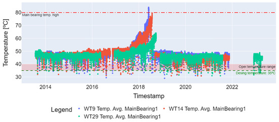
Figure 4.
Main bearing average temperature series with outliers (WT9, WT14, and WT29).
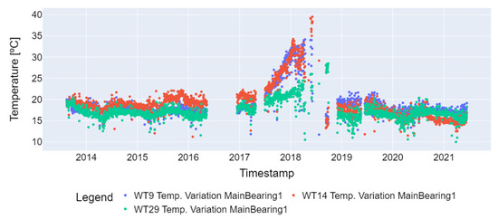
Figure 5.
Temperature variation for the main bearing after outlier removal (WT9, WT14, and WT29).
The final preprocessing step involved applying an additive seasonal decomposition to the time series. This method estimates the time series trend by applying a convolution filter to the data, removing the computed trend from the series, and then calculating the average of the detrended series [18]. In this work, additive seasonal decomposition was used for 7-day periods, and the results are shown in Figure 6.

Figure 6.
Temperature variation for the main bearing after seasonal decomposition (WT9, WT14, and WT29).
2.2. Classification of Temperature Variation Data
This section outlines the process of classifying temperature variation data for application in regression models. The following steps are involved:
- The Identification of Failure Times: A graphical time series analysis determines the first prediction time (FPT) and failure threshold time (FTT). FPT marks the component degradation process initiation, while the FTT signifies complete degradation.
- Minimum Classification Value Definition: A minimum classification value is based on the temperature variation.
- Linear Interpolation: Utilize linear interpolation to classify data between FPT and FTT instances.
In analyzing turbine time series data, essential steps were taken to estimate the remaining useful life (RUL). The failure detection time (FPT) and failure threshold time (FTT) were pinpointed by graphically examining the time series. The FPT represents the beginning of component degradation, and the FTT marks the moment when the component is considered thoroughly degraded. The period between the FTT and FPT is the remaining useful life.
Following data preprocessing (described in Figure 3), the next step is classifying temperature variation data to establish the dependent variable for regression models. A manual definition of the seasonal decomposition stage was carried out by observing the behavior of the temperature variation time series of the main bearing.
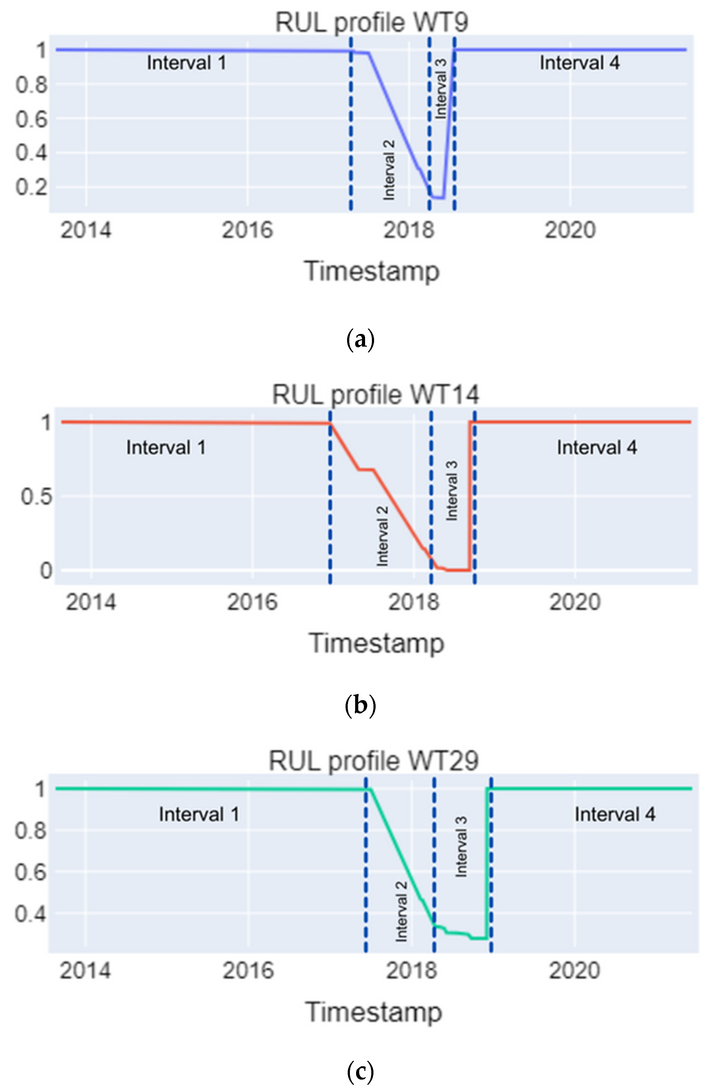
A graphical analysis of the temperature variation time series identified instances of monotonic increase, indicating the FPT. Data before this moment were classified as healthy (assigned the value 1). The FTT, identified as the instant with the most significant temperature variation, represented where data were classified as degraded (assigned the value 0). Upon the return of temperature variation to non-zero values, the data were reclassified as healthy, denoting the restoration of valuable life, referred to as the restoration instant (RT). Each turbine exhibited different maximum temperature variation values: 34.17 °C, 39.5 °C, and 28.5 °C for the WT9, WT14, and WT29 turbines. These values were normalized and employed to define the minimum data classification value according to Equation (1).
Considering the instants FPT, FTT, and RT, along with their corresponding data classification values, linear interpolation was employed to classify temperature variation data within the FPT and FTT intervals. The classification process unfolded across different intervals as follows:
- Interval 1 (Beginning of Time Series to Before Observable Increase in Main Bearing Temperature): Data are consistently classified with a value of one (1).
- Interval 2 (Start of Rise in Main Bearing Temperature to First Occurrence of Maximum Temperature): Values gradually decrease through linear interpolation between 1 and the minimum classification value (Classmin). This considers the interval from the initial rise in main bearing temperature to the point of the first occurrence of the maximum temperature.
- Interval 3 (First Occurrence of Maximum Temperature to Turbine Shutdown): Data classification is assigned a zero value (0) during this interval, extending from the first occurrence of the maximum temperature until the turbine ceases operation.
- Post-Turbine Shutdown and Restart: Upon the resumption of wind turbine operation, the data classification reverts to a value of one (1).
Figure 7 illustrates the comprehensive data classification for the three selected turbines across the entire time series. It showcases distinct degradation dynamics in the main bearings, with variations observed in the degradation speed, which was sometimes faster for WT9 and occasionally slower for WT29.
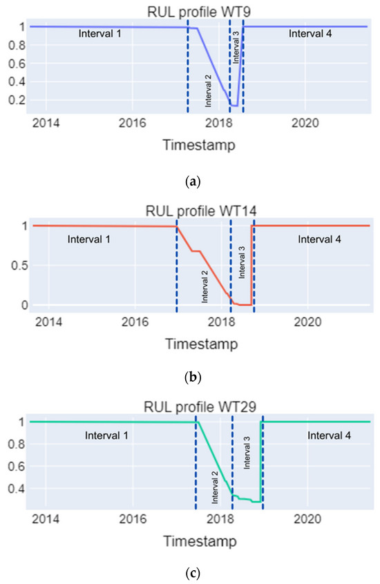
Figure 7.
RUL profiles estimated from the main bearings’ temperature time series for wind turbines (a) WT9, (b) WT14, and (c) WT29.
2.3. Creation of Data Subsets
One common issue with machine learning models is overfitting, which can occur when using samples from the same dataset for training and testing. However, using different datasets involves a trade-off: reducing overfitting at the expense of regression model metrics.
In this study, we employed a strategy to address data scarcity and minimize overfitting, as suggested by [19,20]. This involved using subsets of data, defined through a combination with permutation, from the three-time series of the WT9, WT14, and WT29 turbines, which exhibited the monotonic growth of the main bearing temperature (see Table 1).

Table 1.
Subsets used to deal with the scarcity of data.
The IDs indicated in Table 1 represent a combination of data from one turbine used to train the model (training subset), data from another turbine used to validate the model (validation subset), and data from a third turbine used to test the model after validation (testing subset). These IDs will be used throughout the text to refer to the simulation cases.
2.4. Model Development
Six regressive machine learning models, namely support vector regression (SVR), isotonic regression (ISOR), gradient boosting regression (GBR), decision tree regression (DTR), extra trees regression (ETR), and random forest regression (RFR), were developed to estimate the RUL using the sci-kit-learn Python library.
The training, validation, and test data were normalized according to the respective data ranges (MinMax Scaler) to standardize the range of independent variables [21].
The independent variables used in the models’ training, validation, and testing subsets included the temperature variations of the main bearing, the wind speed, and the net active power of the wind turbines in the subassemblies. The dependent variables were the classified data, shown in Figure 7, estimated from the temperature time series. The data subsets were used as described in Section 2.3 to guarantee the use of distinct subsets for training, validation, and testing.
Cross-validation is a critical process as it enhances the performance of model estimates, reduces overfitting, and aids in selecting the best model and its hyperparameters, thus improving the robustness of tests.
The choice of datasets from different turbines and different power plants aimed to avoid the occurrence of inflated model scores with hyperparameters adjusted through cross-validation, as observed by Leahy et al. [22].
Following the model training, cross-validation was employed to identify the model and hyperparameters that would minimize the mean squared error regression loss. The parameter ranges for each regression model are detailed in Table 2.
Table 2.
List of parameters and ranges of parameters used for cross-validation task.
The following metrics were calculated for each case to evaluate and compare the results of the regression models and are shown in Table 1: mean squared error (MSE), root mean squared error (RMSE), mean absolute error (MAE), and the coefficient of determination (R2 Score). The averages and standard deviations of the training, validation, and test metrics for each subset of the simulated cases were also calculated.
The metrics obtained from the six developed models and the six cases showed slight variations. Consequently, we selected the two models with the lowest MAE values and the R2 Score values closest to 1. The RUL was estimated for each model, and the estimated and observed values were compared, considering the stop dates recorded for the wind turbines, as identified through the main bearing temperature time series.
The calculation of the RUL depends on the availability of information at the first prediction time; in this study, this time was identified using the time series evaluated.
RUL estimates were performed using data from the WT9, WT14, and WT29 turbines. A comparison was then performed with the failure date, also identified in the time series.
3. Analysis and Discussion of Results
This section presents the results obtained with the models at the training, validation, and testing stages. Firstly, the results of the regression model metrics and the selected models are shown. Secondly, the results of the simulations for estimating the RUL are shown. After that, remarks on the RUL estimation results and a discussion about the section results are presented.
3.1. Metrics for Regression Models
Metrics were chosen that allowed for a straightforward interpretation (MAE, MSE, RMSE) to evaluate the regression models that had a lower sensitivity to outliers (MAE) and explained the influence of the independent variables on the dependent variable—RUL— (R2 Score). The lower the MSE and RMSE values, the better the model results. The MAE should vary from 0 to 1 due to the RUL range, with values closer to zero being desirable. Values closer to 1 are desirable for the R2 score.
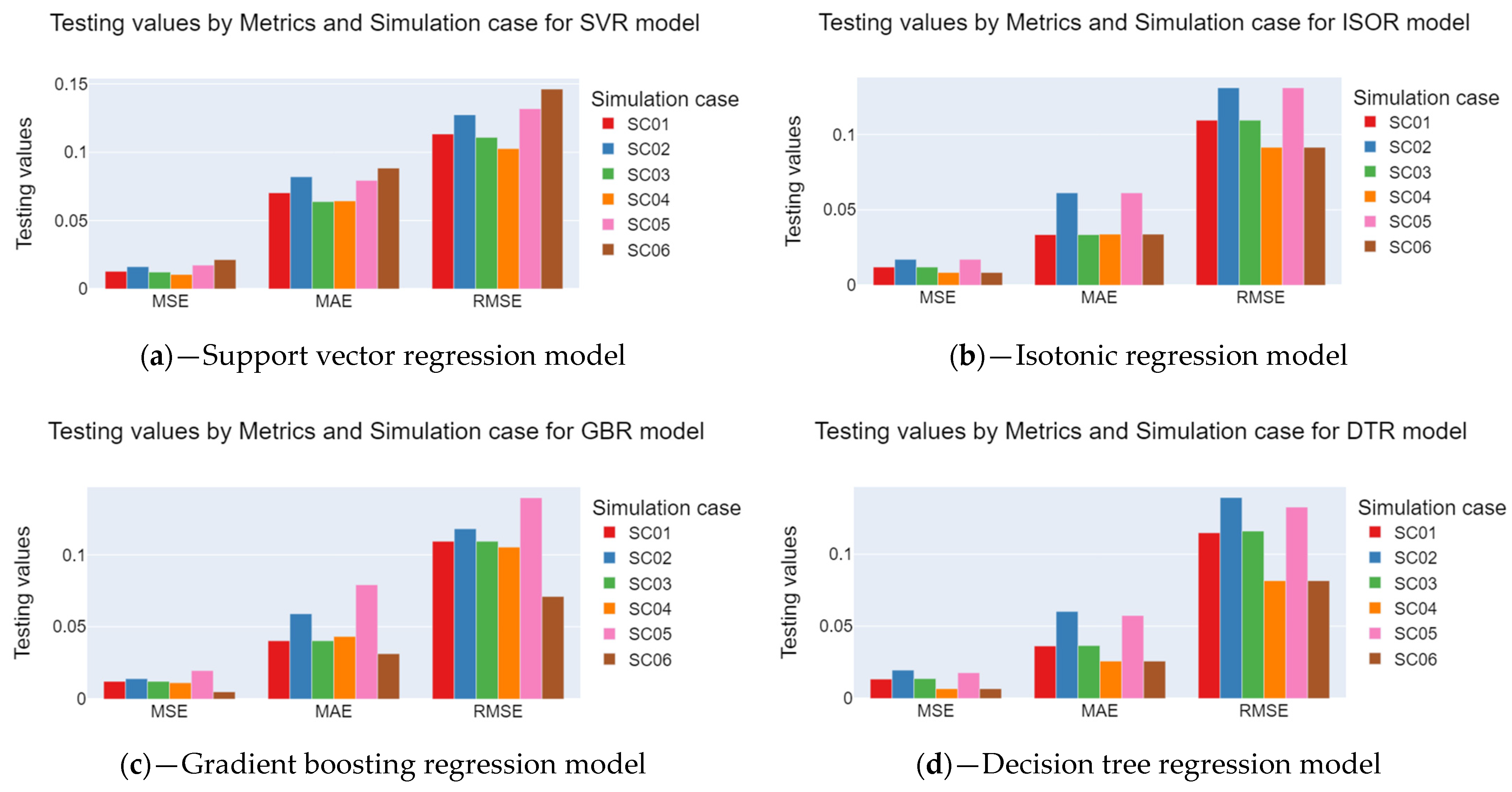
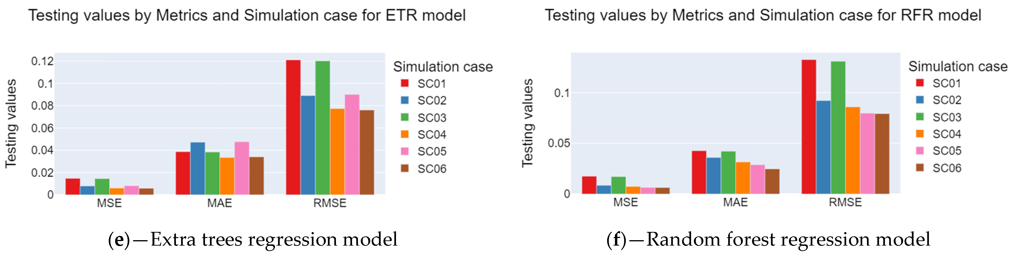
Figure 8 illustrates the average MSE, RMSE, and MAE metric values during the model testing stage. Small variations were observed in the MAE and MSE. Although the average MAE varied from 0.02 to 0.07, the average standard deviation varied between 0.002 and 0.029, indicating that the models must present differences in RUL estimates. The models with the lowest MAE averages were RFR and DTR. The lowest standard deviation values were observed for the GBR, ETR, and DTR models. Consequently, these models should provide estimates with more minor errors, which was proven in the GBR and RFR models, as shown in Section 3.2.
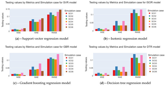
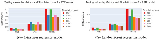
Figure 8.
MAE, MSE, and RMSE results for each regression model and simulation case. (a) support vector, (b) isotonic, (c) gradient boosting, (d) decision tree, (e) extra trees, and (f) random Forest.
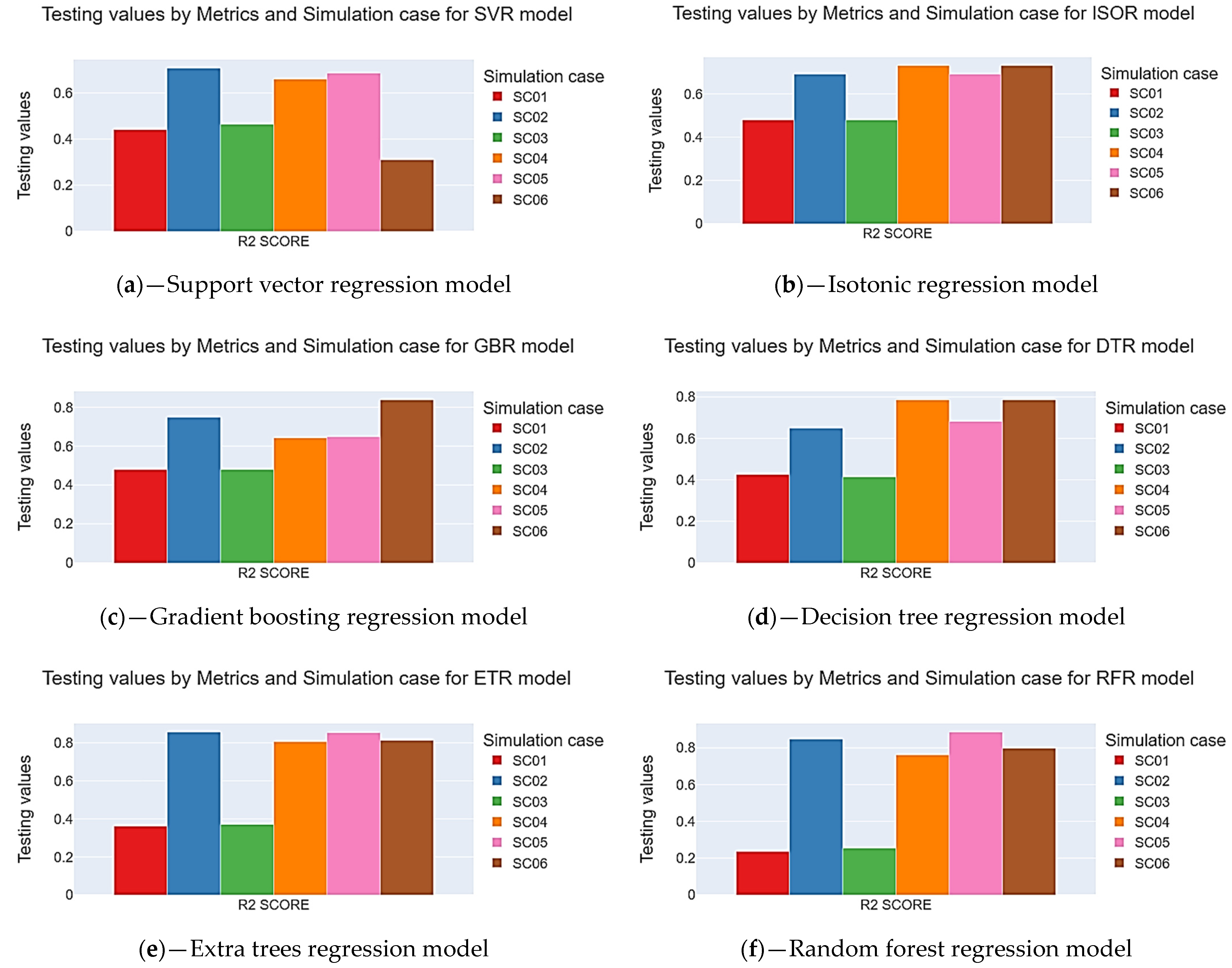
In the case of the R2 Score metric, the average values for the training, validation, and test subsets ranged from 0.894 to 0.639, with a standard deviation ranging from 0.073 to 0.402 (see Figure 9). The RFR, ETR, and GBR models better influenced the main bearing temperature variation on the RUL’s higher R2 Score values. The lowest standard deviation values were observed for the ISOR, ETR, and GBR models. Additionally, the R2 Score results indicate that data subsets 01 and 03 exhibited the lowest values.
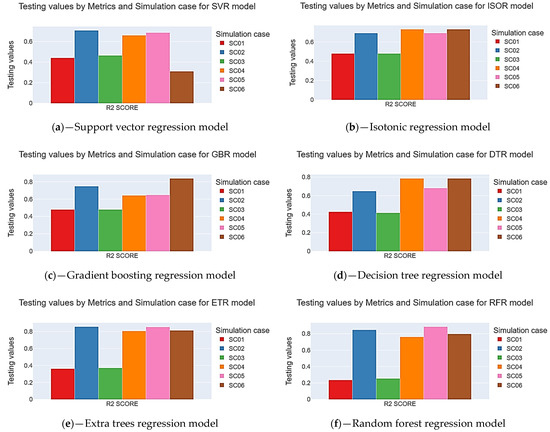
Figure 9.
Results of R2 Score for each regression model and each simulation case. (a) Support vector, (b) Isotonic, (c) Gradient boosting, (d) Decision tree, (e) Extra trees, and (f) Random Forest.
Among the metrics, there was little variation between the training and validation stages:
- For the MAE, the averages ranged from 0.27 in training to 0.25 in validation, Table 3;
Table 3. Results of mean absolute error (MAE) for all simulation cases, for each model, for training, validation, and testing steps.
- For the MSE, the averages ranged from 0.005 in training to 0.004 in validation, Table 4;
Table 4. Mean squared error (MSE) results for all simulation cases, for each model, for training, validation, and testing steps.
- For the RMSE, the averages ranged from 0.066 in training to 0.063 in validation, Table 5;
Table 5. Root mean squared error (RMSE) results for all simulation cases, for each model, for training, validation, and testing steps.
- For the R2 Score, the averages ranged from 0.839 in training to 0.86 in validation, Table 6.
Table 6. Coefficient of determination (R2 Score) results for all simulation cases, for each model, for training, validation, and testing steps.
Ranking the models examined was challenging due to the slight variations across the stages.
Due to the small variation in the MAE averages and the variations in the average and standard deviation of the R2 score, we decided to conduct simulations with all models and evaluate the results by assessing the performances of the models for each simulated case.
3.2. Estimation of the Remaining Useful Life of the Sample Set of Failed Turbines
At this stage, simulations were carried out with the models using the turbine data defined in the test subset for the cases presented in Section 2.3. Table 7 presents the best results obtained in the simulations with the test subsets.
Table 7.
Best simulation results with test subsets.
The “RUL estimation” column indicates the calculated value of the remaining useful life obtained by the respective model and with the respective dataset, and the “Error on RUL estimation” column indicates the differences between the results in the forecast date and date columns when the fault was recorded.
Negative values in the RUL estimation error column indicate that the estimated date was lower than recorded. Positive values in this column indicate that the estimated date was greater than the recorded date.
The results with the SVR and ETR models were obtained without the fault detection date information. The results for the GBR and RFR models were obtained with details on the fault detection date.
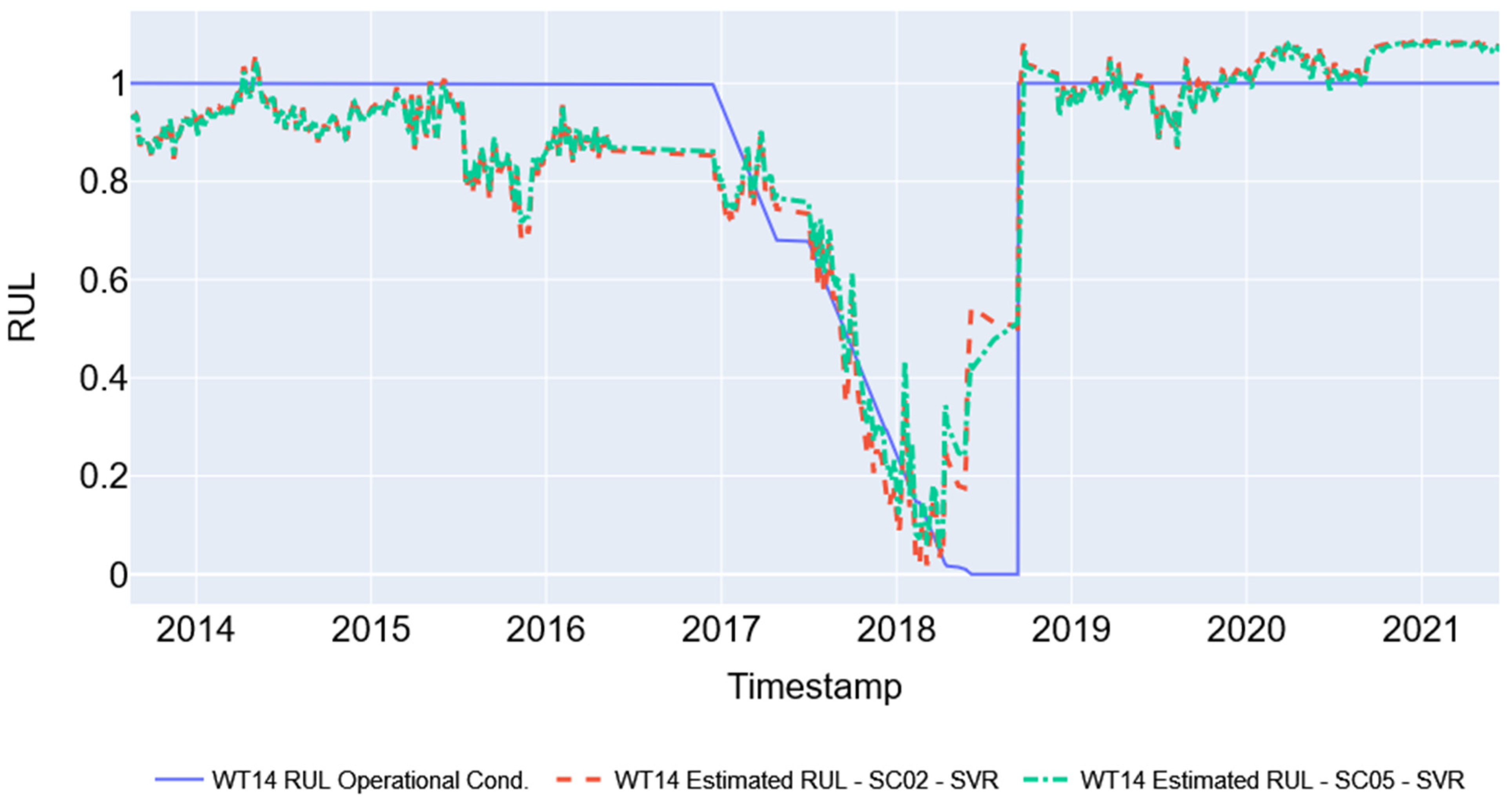
Figure 10 shows the results of the SVR models for the two simulation cases (SC02 and SC05). It is observed that the models, trained and validated with data from other turbines, can represent the behavior of WT14 used in tests until close to the failure date. The model presents more significant errors in making this representation in the interval between stopping and returning to operation.
Figure 10.
Best result simulations with SVR models (SC02 e SC05).
3.3. Remarks on RUL Estimation Results
The developed models demonstrated satisfactory performances for the commonly used metrics used to evaluate regression models. However, the small differences in performance made establishing a ranking strategy for the models challenging.
In the simulations for estimating the RUL, the SVR and ETR models could reproduce the degradation behavior based on the time series data. The SVR model exhibited more conservative results, predicting the failure date earlier than the recorded one.
On the other hand, the GBR and RFR models required information on the date of detection to make a more accurate estimate of the RUL.
3.4. Final Discussion of the Results
The results show that it is possible to estimate RUL using little data and without overfitting, using data from three wind turbines. This makes it a viable complementary option for the decision making of wind farm maintenance managers. However, as highlighted by several authors [21,23,24], intensive real data preprocessing techniques were necessary to obtain time series that would enable obtaining minimally reasonable results from regressive machine learning models. This stage requires the analysis of the mechanical behavior of components, subsystems, and systems under study, combined with data processing techniques to effectively generate useful information for the operation and maintenance of wind turbines.
The results of the remaining useful life estimates (RUL) of wind turbines allow different interpretations from a maintenance point of view. They can be considered assertive, such as the GBR model that predicted the date with an error of zero days; conservative, in the case of SVR models that underestimated the useful life; and non-conservative, such as the ETR and RFR models, which overestimated the values found in the time series (see Table 7). Therefore, conservative estimates, such as those from the SVR, and assertive ones, such as those from the GBR, can support proper maintenance planning for the resources needed to carry out scheduled shutdowns and interventions on the turbines, thus avoiding catastrophic failures that could reduce the availability of the wind farm. In this way, the estimates support the prevention of catastrophic faults and guarantee the operation of the turbines [25]. In the same context, using subsets of real data effectively mitigated the effects of scarce data and overfitting, which was a significant contribution due to the limited availability of time series data on main bearing failures.
The strategy of creating simulation cases proved effective in dealing with the issue of data scarcity without the need to use data padding or synthetic data. Future work could address the development of a framework that uses data of increasing complexity (synthetic data, bench test data, and real data) to enable the use and evaluation of different machine learning or deep learning models.
Nevertheless, for the successful application of the method, data on the variables of interest, indicated in Section 2.1, are necessary from at least three wind turbines that have experienced main bearing failure to minimize overfitting. Another limitation of the method is the need for main bearing temperature data with monotonic growth and, if possible, with records close to the turbine shutdown date for replacements. Using low-temperature values for model training and validation may bias the results, and the method may indicate a replacement before the component’s actual end of life.
It is worth underscoring that utilizing low-temperature values during the model’s training and validation can introduce distortion into the results. Such a bias may cause the method to suggest replacement prematurely, preceding the actual conclusion of the component’s operational lifespan. Therefore, meticulous and representative data collection is imperative to uphold the dependability and precision of the analysis, preventing premature or erroneous determinations in the context of main bearing replacement.
4. Conclusions
A framework for predicting wind turbine main bearing failures was developed and tested using temperature data from a SCADA system. Temperature data and different machine learning regression models (support vector regression isotonic regression, gradient boosting regression, decision tree, extra trees, and random forest regression) were used to estimate the remaining useful life (RUL) of the main bearings of wind turbines with scarce data. The main findings of the study are as follows:
- The models were tested on real data from three wind turbines in northeastern Brazil, showing satisfactory results in each step of the validation and test. The MAE, MSE, RMSE, and R2 Score metric values in the validation step were 0.25, 0.004, 0.004, and 0.86, respectively;
- Regarding the simulation, the results demonstrated that the models (SVR, ETR, GBR, and RFR) outperformed since they showed an average of 20 days in estimating the remaining useful life of the main bearings of the wind turbines;
- The methodology showed that conservative estimates, such as those from the SVR, and assertive ones, such as those from the GBR, can support proper maintenance planning, thereby avoiding catastrophic failures that could reduce the wind farm’s availability.
Future work will focus on developing a framework that uses synthetic, bench, and real data to build more complex models. It is also essential to understand the failure mechanisms and the data collection process for model development, as indicated by [2,26]. Furthermore, organizations must improve data management processes for effective decision making [26].
Author Contributions
Conceptualization, J.L.d.M.V., F.C.F., and G.d.N.P.L.; methodology, J.L.d.M.V., G.d.N.P.L. and A.A.V.O.; software, J.L.d.M.V., F.C.F., G.d.N.P.L. and A.A.V.O.; validation, J.L.d.M.V. and G.d.N.P.L.; formal analysis, J.L.d.M.V.; investigation, J.L.d.M.V.; resources A.A.V.O., J.Â.P.d.C., F.D.d.M., A.C.A.d.C., M.G.G.d.S. and G.d.N.P.L.; data curation, J.L.d.M.V., O.d.C.V. and M.G.G.d.S.; writing—original draft preparation, J.L.d.M.V., P.S.A.M., and A.A.V.O.; writing—review and editing, J.Â.P.d.C., P.S.A.M., G.d.N.P.L., and A.A.V.O.; visualization, P.S.A.M.; supervision, J.Â.P.d.C., G.d.N.P.L., A.A.V.O. and P.S.A.M.; project administration, A.C.A.d.C., J.Â.P.d.C., G.d.N.P.L., A.A.V.O., M.G.G.d.S. and P.S.A.M.; funding acquisition, A.C.A.d.C., J.Â.P.d.C., G.d.N.P.L., M.G.G.d.S., O.d.C.V. and A.A.V.O. All authors have read and agreed to the published version of the manuscript.
Funding
This research was funded by Rio Amazonas SA—2021.
Data Availability Statement
The data are not publicly available due to confidentiality issues.
Acknowledgments
This study obtained information while developing a Research and Development—R&D project supported by Rio Amazonas SA and approved by the Brazilian Regulatory Agency ANEEL. The first author thanks IFPE, Brazil, for the support through their doctorate thesis. The third author thanks CNPq, Brazil, for the support through productivity grant n. 303417/2022-6. The seventh author thanks CNPq for his support through post-doctorate grant 200820/2022-2 under Call 26/2021 and productivity grant n. 303200/2023-5. The third, fourth, sixth, and seventh authors thank IFPE for the financial support under Call REI/IFPE No. 43/2023.
Conflicts of Interest
Author Marrison Gabriel Guedes de Souza was employed by the company NEOG, Brazil. The remaining authors declare that the research was conducted in the absence of any commercial or financial relationships that could be construed as a potential conflict of interest.
References
- Strielkowski, W.; Civín, L.; Tarkhanova, E.; Tvaronavičienė, M.; Petrenko, Y. Renewable Energy in the Sustainable Development of Electrical Power Sector: A Review. Energies 2021, 14, 8420. [Google Scholar] [CrossRef]
- de Novaes Pires Leite, G.; Araújo, A.M.; Rosas, P.A.C. Prognostic Techniques Applied to Maintenance of Wind Turbines: A Concise and Specific Review. Renew. Sustain. Energy Rev. 2018, 81, 1917–1925. [Google Scholar] [CrossRef]
- Guo, Y.; Sheng, S.; Phillips, C.; Keller, J.; Veers, P.; Williams, L. A Methodology for Reliability Assessment and Prognosis of Bearing Axial Cracking in Wind Turbine Gearboxes. Renew. Sustain. Energy Rev. 2020, 127, 109888. [Google Scholar] [CrossRef]
- BS EN 13306:2010; Maintenance—Maintenance Terminology. NSAI. 2010. Available online: https://www.en-standard.eu/bs-en-13306-2017-maintenance-maintenance-terminology/?gad_source=1&gclid=Cj0KCQjwwMqvBhCtARIsAIXsZpZS1xtdpaIhepDSfK9Ukr8llB0tSP-j860QQhjm2l81JU8jXHbnnDIaAu1TEALw_wcB (accessed on 17 January 2024).
- Randall, R.B. Vibration-Based Condition Monitoring, 1st ed.; John Wiley & Sons, Ltd: Hoboken, NJ, USA, 2011; ISBN 9780470747858. [Google Scholar]
- Koukoura, S. Failure and Remaining Useful Life Prediction of Wind Turbine Gearboxes. Annu. Conf. PHM Soc. 2018, 10. [Google Scholar] [CrossRef]
- Carroll, J.; Koukoura, S.; McDonald, A.; Charalambous, A.; Weiss, S.; McArthur, S. Wind Turbine Gearbox Failure and Remaining Useful Life Prediction Using Machine Learning Techniques. Wind Energy 2019, 22, 360–375. [Google Scholar] [CrossRef]
- Dameshghi, A.; Refan, M.H. Combination of Condition Monitoring and Prognosis Systems Based on Current Measurement and PSO-LS-SVM Method for Wind Turbine DFIGs with Rotor Electrical Asymmetry. Energy Syst. 2021, 12, 203–232. [Google Scholar] [CrossRef]
- Herp, J.; Pedersen, N.L.; Nadimi, E.S. Assessment of Early Stopping through Statistical Health Prognostic Models for Empirical Rul Estimation in Wind Turbine Main Bearing Failure Monitoring. Energies 2019, 13, 83. [Google Scholar] [CrossRef]
- Elasha, F.; Shanbr, S.; Li, X.; Mba, D. Prognosis of a Wind Turbine Gearbox Bearing Using Supervised Machine Learning. Sensors 2019, 19, 3092. [Google Scholar] [CrossRef] [PubMed]
- Hart, E.; Clarke, B.; Nicholas, G.; Kazemi Amiri, A.; Stirling, J.; Carroll, J.; Dwyer-Joyce, R.; McDonald, A.; Long, H. A Review of Wind Turbine Main Bearings: Design, Operation, Modelling, Damage Mechanisms and Fault Detection. Wind Energy Sci. 2020, 5, 105–124. [Google Scholar] [CrossRef]
- Yucesan, Y.A.; Viana, F.A.C. A Hybrid Model for Main Bearing Fatigue Prognosis Based on Physics and Machine Learning. In Proceedings of the AIAA Scitech 2020 Forum, Orlando, FL, USA, 6–10 January 2020; American Institute of Aeronautics and Astronautics Inc., AIAA: Orlando, FL, USA, 2020; Volume 1. Part F. [Google Scholar]
- Yucesan, Y.A.; Viana, F.A.C. Wind Turbine Main Bearing Fatigue Life Estimation with Physics-Informed Neural Networks; PHM Society: Orlando, FL, USA, 2019. [Google Scholar]
- Yang, L.; Zhang, Z. Wind Turbine Gearbox Failure Detection Based on SCADA Data: A Deep Learning Based Approach. IEEE IEEE Trans. Instrum. Meas. 2020, 70, 3507911. [Google Scholar] [CrossRef]
- Hu, C.; Byeng, D.Y.; Youn, D.; Wang, P. Springer Series in Reliability Engineering Design under Uncertainty and Health Prognostics; Springer Publisher: New York, NY, USA, 2019. [Google Scholar]
- Wiese, B.; Pedersen, N.L.; Nadimi, E.S.; Herp, J. Estimating the Remaining Power Generation of Wind Turbines—An Exploratory Study for Main Bearing Failures. Energies 2020, 13, 3406. [Google Scholar] [CrossRef]
- McKinney, W. Pandas: A Python Data Analysis Library. Available online: http://pandas.sourceforge.net (accessed on 17 January 2024).
- Perktold, J.; Seabold, S.; Taylor, J. Statsmodels Documentation. Available online: https://www.statsmodels.org/stable/generated/statsmodels.tsa.seasonal.seasonal_decompose.html#statsmodels.tsa.seasonal.seasonal_decompose (accessed on 17 January 2024).
- Rezamand, M.; Carriveau, R.; Ting, D.S.K.; Davison, M.; Davis, J.J. Aggregate Reliability Analysis of Wind Turbine Generators. IET Renew. Power Gener. 2019, 13, 1902–1910. [Google Scholar] [CrossRef]
- Abid, K.; Sayed-Mouchaweh, M.; Laurence, C. Adaptive Machine Learning Approach for Fault Prognostics Based on Normal Conditions—Application to Shaft Bearings of Wind Turbine. Annu. Conf. PHM Soc. 2019, 11, 46–50. [Google Scholar] [CrossRef]
- Tutiv’en, C.; Benalcazar–Parra, C.; Escuela, A.E.; Vidal, Y.; Puruncaias, B.; Fajardo, M. Wind Turbine Main Bearing Condition Monitoring via Convolutional Autoencoder Neural Networks. In Proceedings of the 2021 International Conference on Electrical, Computer, Communications and Mechatronics Engineering (ICECCME), Mauritius, 7–8 October 2021; pp. 1–6. [Google Scholar]
- Leahy, K.; Gallagher, C.; O’Donovan, P.; Bruton, K.; O’Sullivan, D.T.J. A Robust Prescriptive Framework and Performance Metric for Diagnosing and Predicting Wind Turbine Faults Based on SCADA and Alarms Data with Case Study. Energies 2018, 11, 1738. [Google Scholar] [CrossRef]
- Zhao, Y.; Li, D.; Dong, A.; Kang, D.; Lv, Q.; Shang, L. Fault Prediction and Diagnosis of Wind Turbine Generators Using SCADA Data. Energies 2017, 10, 1210. [Google Scholar] [CrossRef]
- Correa-jullian, C.; Cofre-martel, S.; Martin, G.S.; Droguett, E.L.; de Novaes Pires Leite, G.; Costa, A. Exploring Quantum Machine Learning and Feature Reduction Techniques for Wind Turbine Pitch Fault Detection. Energies 2022, 15, 2792. [Google Scholar] [CrossRef]
- Sahu, A.; Jambhale, R.; Adiga, D.T.; Powar, N.; Mckinley, T. Formulation of Model Stability Metrics for Remaining Useful Life Models of Engine Components. In Proceedings of the 2023 IEEE Aerospace Conference, Big Sky, MT, USA, 4–11 March 2023; Volume 2023, pp. 1–11. [Google Scholar]
- Sikorska, J.Z.; Hodkiewicz, M.; Ma, L. Prognostic Modelling Options for Remaining Useful Life Estimation by Industry. Mech. Syst. Signal Process. 2011, 25, 1803–1836. [Google Scholar] [CrossRef]

Disclaimer/Publisher’s Note: The statements, opinions and data contained in all publications are solely those of the individual author(s) and contributor(s) and not of MDPI and/or the editor(s). MDPI and/or the editor(s) disclaim responsibility for any injury to people or property resulting from any ideas, methods, instructions or products referred to in the content. |
© 2024 by the authors. Licensee MDPI, Basel, Switzerland. This article is an open access article distributed under the terms and conditions of the Creative Commons Attribution (CC BY) license (https://creativecommons.org/licenses/by/4.0/).