
Fluid–Solid Mixing Transfer Mechanism and Flow Patterns of the Double-Layered Impeller Stirring Tank by the CFD-DEM Method
1
Special Equipment Institute, Hangzhou Vocational and Technical College, Hangzhou 310018, China
2
College of Mechanical and Automotive Engineering, Zhejiang University of Water Resources and Electric Power, Hangzhou 310018, China
*
Author to whom correspondence should be addressed.
Energies 2024, 17(7), 1513; https://doi.org/10.3390/en17071513
Submission received: 2 February 2024
/
Revised: 29 February 2024
/
Accepted: 12 March 2024
/
Published: 22 March 2024
Abstract
:The optimization design of the double-layered material tank is essential to improve the material mixing efficiency and quality in chemical engineering and lithium battery production. The draft tube structure and double-layered impellers affect the flow patterns of the fluid–solid transfer process, and its flow pattern recognition faces significant challenges. This paper presents a fluid–solid mixing transfer modeling method using the CFD-DEM coupling solution method to analyze flow pattern evolution regularities. A porous-based interphase coupling technology solved the interphase force and could be used to acquire accurate particle motion trajectories. The effect mechanism of fluid–solid transfer courses in the double-layered mixing tank with a draft tube can be obtained by analyzing key features, including velocity distribution, circulation flows, power, and particle characteristics. The research results illustrate that the draft tube structure creates two major circulations in the mixing transfer process and changes particle and vortex flow patterns. The circulating motion of the double-layered impellers strengthens the overall fluid circulation, enhances the overall mixing efficiency of the fluid medium, and reduces particle deposition. Numerical results can offer technical guidance for the chemical extraction course and lithium battery slurry mixing.
1. Introduction
With continuous industrial development, stirred reactors are frequently used in industrial productions, including petroleum, chemical, metallurgy, pharmaceuticals, polymers, and food. The agitator is one of the core components of a stirred reactor, which is capable of achieving the efficient and uniform mixing of fluids or the uniform dispersion of multiphase fluids [1,2,3]. Different fluid media under the rotation of the impeller blades exhibit a turbulent reciprocating state as a whole, but there is strong random flow internally [4,5]. Mass transfer and diffusion among different media eventually reach an equilibrium state. The internal structure of the mixing tank, such as the number of impeller layers and the draft tube, greatly influences the flow field distribution and energy conversion efficiency within the tank. When materials are mixed in the stirring kettle, it is necessary to consider not only the mixing inside the kettle but also the effect of the impeller blades on the medium within the kettle. A rotation speed that is too high can damage the medium, affecting the preparation of chemical raw materials, while a speed that is too low affects the mixing of materials [6,7,8]. Therefore, studying the mixing flow mechanism and flow patterns of solid–liquid biphasic fluids in a double-layered mixing tank with a draft tube has significant scientific value and prospects for engineering applications.
For the mixing tank with a draft tube, the layout of the draft tube is crucial, and a position close to the tank bottom increases pressure pulsation phenomena. The draft tube is fitted with an axial flow impeller that transports the fluid downwards or upwards while creating an upward or downward backflow between the draft tube and the mixing tank. The draft tube not only intensifies fluid stirring but also establishes the circulation flow pattern within the mixing tank [9,10]. When using an impeller for solid–liquid mixing, the draft tube allows for the uniform mixing of the fluid between the top and bottom of the tank, enabling a higher flow rate per unit power of the mixing equipment [11,12,13]. However, the presence of the draft tube makes the material mixing process more complex, as the mixing transport process and flow patterns exhibit a high degree of randomness. Therefore, researching the mixing flow mechanism of solid–liquid biphasic fluids in a double-layered mixing tank with a draft tube presents significant challenges [14,15].
In response to the above issues, numerous studies have been conducted by scholars, yet research on stirred reactors with draft tubes remains relatively limited. Zhang set up the reactive transport model to discuss oil multi-field coupling evolution regularities and found that multiple species transport and morphology are influenced by hydraulic drop and media connectivity [16]. Ramezani added ethanol surfactants to a vortex reactor to study the distribution and shape of bubbles within the reactor, providing a valuable reference for researching the overall and local gas content distribution within reactors [17]. Scargiali investigated the impact of impeller structures on mass transfer performance under critical and non-critical conditions, finding that mass transfer in systems without baffles is primarily influenced by power [18]. John measured the stirring power of a double-layered agitator system with a draft tube and found that introducing the baffle increased the power number [19]. Li researched the gas–liquid–solid system in the stirring tank with a draft tube but without a baffle structure, discovering that the draft tube led to increasing stirring power [20].
The aforementioned studies revealed that current research primarily focuses on bubble morphology, mixing mass transfer, and power measurement. In unbaffled stirred tanks, the liquid exhibits a strong circumferential rotation, leading to a concave gas–liquid free surface around the stirrer axis at the tank center, which results in a reduction in the measured stirring power. The lack of accurate modeling and solving methods for the fluid–solid mixing flow mechanism with draft tube structures makes it challenging to reveal flow pattern evolution regularities.
This paper proposes a fluid–solid mixing transfer modeling approach in double-layer stirred tanks. A three-dimensional mixing dynamics model based on CFD-DEM coupling is set up, combined with the SST turbulence model, to explore multiphase transfer mechanisms and flow patterns. Flow pattern evolution in the mixing field is explored by analyzing the impeller rotation. The research findings can offer helpful guidance and technical support for industrial production processes such as chemical material mixing, lithium battery slurry mixing, and food processing.
2. Mathematical Model of the Solid–Liquid Mixing Process
2.1. Mathematical Model of the Fluid Field
Based on multiphase mixing and multi-field coupling, the stirred reactor is taken as the object of study. The multiphase flow velocity field within the stirring tank is interrelated with each phase. It is assumed that the gas–liquid two-phase is an incompressible viscous fluid. The momentum balance equations and continuity equations for liquids and solids describe the dynamic features of each phase, with each phase sharing the same pressure and velocity fields [21,22]. The continuous-phase fluid is viscous and incompressible, and the liquid-phase continuity equation is as follows:
where V represents the control volume, and A represents the control surface. For the continuity changes in the liquid phase, there is no flow loss in the middle of the reactor, and no leakage occurs in the middle of the container; thus, the liquid-phase flow conforms to continuity equations [23,24,25]. Momentum conservation equations are expressed as follows:
where ρi and μi describe the fluid density and viscosity, respectively, g is the gravity, u is the fluid velocity vector, t is the time, p is the fluid pressure, and fs is the surface tension force [26,27].
A turbulence model requires a comprehensive consideration of the features of fluid flow, accuracy, and computation time [28,29,30]. The Reynolds-averaged Navier–Stokes method, which is capable of describing the most essential time-averaged information in turbulent fields with lesser computational demands, is widely applied in engineering. The internal turbulence effects in the stirring tank are modeled using the RNG k-ε model [31,32]. The above model facilitates turbulent conditions of multiphase flows, aligning well with the study of the internal flow fields.
where Gk, Gb, and YM are the terms for turbulent kinetic energy production. Variables αk and αε represent the inverses of adequate Prandtl numbers, respectively [33,34,35]. The other empirical parameters used in this paper are as follows: C1ε = 1.44, C2ε = 1.92, C3ε = 0.09, σk = 1.0, and σε = 1.3. The RNG k-ε model can be applied to study high Reynolds number turbulent flow phenomena, particularly rapid strain, medium-scale vortices, and complex shear flows with local transition [36,37]. The internal mixed flow in the stirred tank studied in this paper involves addressing flow separation and complex secondary flows. This model suits the numerical swirl simulation within the stirring tank.
2.2. Particle Dynamics Model
In liquid–solid flows, solid particles are taken on in a turbulent state, leading to coupling effects among various factors, resulting in a nonlinear and complex flow of particles in the flow field [38,39,40]. Here, with no mass transfer between solid and liquid phases, fluid phase control equations should consider the volume fraction αf occupied by solid particles in the grid cell, where Fa is the interphase force, and S is the average force exerted on the particles.
where n and Vf represent the number of solid particles and cell volume. Here, the fluid control equation is modified as follows:
where ρf and vf represent the density and velocity of fluid phases, and f denotes the stress–strain tensor.
where ηf and λf represent the shear viscosity and bulk viscosity, and represents the turbulence kinetic energy.
Based on control equations, it is possible to obtain the liquid phase velocity and pressure fields in the stirred tank reactor’s flow field. This solution provides initial conditions for the motion of solid particles [41,42,43].
The reactor is analyzed with individual solid particles as the subject, which are tracked in a Lagrangian manner within the DEM framework, with its dynamic equation as follows:
where FC and G represent the individual contact force and gravity. Particle motion results from multiple forces, including the drag (Fd), pressure gradient (Fp), Basset force (Fb), Saffman force (Fs), Magnus lift (Fm), buoyancy (Ff), and added mass force (Fv). The force situation of a single particle in the flow field is illustrated in Figure 1.
During the chemical reaction course, the density of the liquid is lower than the density of the particles, and the virtual mass force and Basset force are deleted. Thus, the equation can be expressed as follows:
where the method for solving the drag force is
where ρp, vp, and dp represent the density, velocity, and diameter. Cd and Rep denote the drag coefficient and Reynolds number [44,45,46], with their expressions as follows:
where μf represents the dynamic viscosity of the liquid phase. The gradient pressure, Saffman lift force, and Magnus lift force are obtained, respectively:
where θ(R) represents the residual term. Considering the mutual interactions among solid particles in the reactor, we employed the Hertz–Mindlin soft-sphere model for calculations [47,48,49,50]. During flow processes, there are contact collisions between particles, and the force equation for particle collisions is as follows:
where Fn represents the normal contact force, where the soft-sphere model replaces the particle’s normal contact process with a spring and damper. Ft represents the tangential contact force, where the tangential contact process is replaced with a spring, damper, and slider in the model.
2.3. Fluid–Solid Coupling Solution Method
To obtain the interaction forces, a porous-based interphase coupling technology can be used to acquire accurate particle motion trajectories. This model overcomes the computational instability issues caused by traditional methods when the particle size approaches the grid size, thus improving the particle–fluid interaction. The control equations are written into interface programs for compilation. Ultimately, bidirectional coupling is achieved. Thus, a CFD-DEM calculation facilitates data transfer by the user-defined functions (UDF), realizing bidirectional coupling between the Eulerian dual-fluid phase and the Lagrangian particle phase.
The overall computational workflow of the model is depicted in Figure 2. The fluid fields and particles are initialized. The flow field’s velocity and force are determined by iteratively solving control equations. The DEM module iteratively calculates the velocity and position of the particles. The decision on whether to continue is based on a convergence assessment. If not converged, the porosity of the fluid element is determined to continue the flow field calculations. This cycle, which achieves bidirectional coupling through data exchange, continues until convergence is reached, at which point the computations stop, and the calculation can be completed.
3. Numerical Model of Fluid–Solid Mixing Tank
3.1. Numerical Dynamic Model
The thorough mixing of material liquid using stirring equipment involves the transfer of kinetic energy, heat, and mass. The sealed nature of the stirring container affects the flow state of the gases involved in the reaction, indirectly influencing the yield of the reaction products. Figure 3 presents a schematic of the three-dimensional structure of a double-layered stirring tank with a guide cylinder, including the draft tube, double-layer blades, and an elliptical bottom for sealing the stirring container. Figure 3 depicts the stirring impeller. While the structures near the impellers are complex, minor details do not significantly alter the flow patterns. Therefore, for the structural schematic of the stirring tank, simplifications have been made at the connection between the impeller and the shaft and at the top hole of the tank to facilitate the relevant grid division and numerical calculations.
Owing to the large size of the stirring tank compared to the much smaller rotating blades, the significant difference in their scales poses considerable challenges for precise grid division. The numerical model is shown in Figure 4. For the small-sized mixing impellers in the strong shear flow region (Figure 4b), unstructured meshes are used to divide blade structures and refine the blade. The mesh size is 0.003 mm with a total of 1,825,740 grids, and the grid quality is above 0.8. For the rest of the three-dimensional stirring tank’s fluid domain, an unstructured grid with a scale of 0.01 mm is used, totaling 1,395,515 grids with a quality above 0.6. The grid size in this part can be larger than that of the blades (Figure 4a,c), which can enhance calculation speeds. The mesh quantity can ensure the computational accuracy requirements are met.
To address the particulate phase, the physical models must be imported under the EDEM 2.7 software. The finer the grid division, the higher the computation efficiency and accuracy of the results. Consequently, the computational area is divided into grid cells of specific scales, with particles distributed throughout the container and solely influenced by gravity. During the fluid–solid-coupled calculation, the solver determines the motion equation of the particles by calculating the interactive forces and contact forces. It continuously updates the position of the particles, tracking their flow state.
3.2. Solution Conditions
The solid–liquid simulation employs a transient Eulerian model with an explicit time discretization format chosen. The RNG turbulent model is used for turbulence modeling, providing accurate solutions for the mixed turbulence process, with standard wall functions selected for near-wall regions. The container top is a pressure outlet. The convergence residuals monitored are all at 10−6. The multiple reference frame method allows for transient simulation, offering greater accuracy than the sliding grid method and saving substantial computational resources [51]. Its accuracy satisfies the needs of most scenarios. Here, this calculation employs the multiple reference frame method, with data transmission occurring through the interface between these two areas.
3.3. Mesh Independence Results
Mesh numbers influence computing results; as the mesh numbers rise, the calculation precisions improve, but the computational efficiency decreases. Here, it is essential to determine the appropriate mesh, meaning that grid independence verification should yield relatively accurate calculation results while maximizing computational efficiency. In the grid independence verification, the impeller is taken as the subject, with grids totaling 2,362,500, 3,221,225, and 4,523,120 divided. After the calculations have converged, the average velocity distribution under the three grid quantities is compared.
In Figure 5, the average velocities for variable grid quantities are not significantly different. The maximum velocity error between grid counts 4,523,120 and 3,221,225 is 1.2%, while the maximum velocity error between grid counts 3,221,225 and 2,362,500 is 4.7%. Therefore, the numerical model with 3,221,225 grids can meet the requirements for computational accuracy while ensuring a faster calculation rate.
4. Results and Discussions
4.1. Formation Regularities of Leaf Rotation Fields
Mixing flows inside the stirring tank os complex, and turbulent hydrodynamic phenomena are characterized by highly nonlinear transport processes. This study focuses on a stirring tank with double-layered impeller blades and a draft tube, conducting a numerical simulation to calculate the characteristics of the draft tube and analyze the simulation results. Figure 6 illustrates the velocity cloud chart in the draft tube stirring tank. The observation of the velocity cloud diagram reveals that under the action of the rotating blades, the recirculation of fluid within the tank is symmetrical, and the fluid mixing process is intense. The high-speed area indicates that during the stirring course, the impeller, due to its higher flow velocity, achieves a better degree of material mixing compared to the external flow field. In Figure 6, the double-layered stirring blades within the draft tube stirring tank show an effective mixing result, leading to the more thorough mixing of the fluid inside the tank. However, due to factors such as stirring speed and blade structures, the blades exhibit significant changes in the velocity gradient. By contrast, mixing fields away from the blades shows little variation in velocity.
Impeller velocity cloud diagrams over various times are shown in Figure 7. By comparing the upper and lower impellers, the uniformity of the velocity gradually increases. Due to the larger inclination angle of the lower blades compared to the upper blades, the velocity gradient changes in the flow field of the lower blades are pronounced. The outer ends of the blades have a stronger ability to disturb the flow field, which is reflected on the side as a better effect of material mixing. However, the correlation between the adjacent two layers of the blades is not enhanced; instead, there is an increase in the radial flow. Hence, in material mixing, it can be considered that an appropriate increase in the blade inclination angle is of significant importance for improving the efficiency of chemical mixing.
4.2. Calculation of Circulating Flows
The circulation action involves the continuous exchange of fluid microelements between high- and low-shear areas. As the particle dissolution progresses, the circulation flow significantly decreases, and consequently, the mixing rate also reduces with the decreased circulation flow. Therefore, enhancing the circulation capability is a primary means to increase the mixing rate of the fluid. The specific calculation involves obtaining the circulation flow by integrating the velocity across the surface passing through the vortex core:
where r* denotes the vortex center location, R is the slot radius, and vr is the corresponding velocity vector.
The mixing fields have two major circulations, symmetrically distributed around the axis. By calculating the circulation flow of one side and then doubling it, the overall circulation flow can be obtained. There are two small circulations in the upper part of the stirring tank, which are almost negligible compared to the major circulations, so only the right-side major circulation needs to be calculated. The vortex core of the right-side major circulation was determined through observations and measurements to have the coordinates (0.75, −1.5). The radial velocity could be obtained (Figure 8b). The discrete data of v-r were imported into MATLAB for calculation, yielding a total circulation flow of QC = 3.0526 m/s3 at t = 4 s. The fluid within the draft tube was accelerated by the action of the double-layered blades, increasing the fluid velocity. A small part of the fluid (at the bottom center) touched the bottom and then turned upwards into the draft tube, while the fluids moved upwards along the draft tube outside and flowed toward the tank top. Clearly, the double-layered stirring blades and draft tube in the stirring tank better facilitate mixing different fluids.
Simultaneously, in dead-zone volumes, the inclined blades of the lower impeller reduce the dead-zone volume. After the blades are inclined, they create a radial pumping effect, causing part of the fluid to change from an axial to radial flow. The greater the inclination angle of the blades, the more pronounced the radial pumping effect becomes, enhancing the circulation. When the rising fluid reaches a certain height, it splits into two streams. After moving radially to the wall position, each stream flows downward along the wall. Upon encountering the fluid radially pumped by the blades, the two streams merge and continue to flow down along the wall to the bottom of the kettle. Then, they are drawn by the rotating blades and continue to move upward, forming a circulation.
4.3. Power Calculation of Impeller Shaft
In this study, influenced by the wall pressure load and fluid viscosity, the methods for analytical solutions of torque and the power of stirring impellers were complex and had limited practical application. Despite extensive research, there is no academic consensus or universally applicable analytical solution method for industrial production. In contrast, the numerical method based on one-way fluid–solid coupling has more advantages in solving this problem. This method is to apply the pressure load and viscous forces to the solid domain, thereby deriving the force vectors on the impeller at each micro-element grid. The shaft power can be calculated by integrating the torque over the impeller surface and combining it with the rated speed.
Based on the above method, the changes in torque at different times during the stirring process for both the upper and lower impellers were obtained. The distribution of the impeller pressure load is shown in Figure 9 and Figure 10, and the torque is presented in Table 1. The pressure loads in Figure 9 and Figure 10 are only used as the basis for changes in the structural field force vectors, and changes in the flow field due to the forced deformation of the structure are not considered. During the stirring process, the impeller surface pressure load varies significantly due to fluid inertial forces, particle settling, and bottom-blowing effects. From a temporal perspective, the torque due to the pressure load on the upper impeller initially decreases, then increases, and finally decreases again. This is mainly because, at the start of stirring, the impeller needs to work against fluid inertial forces. As the stirring continues, the rotational speed in the impeller’s area increases, reducing the inertial forces.
After obtaining the impeller torque, the power requirements can be determined. The power of the impellers can be obtained in Figure 11. The power range is 7~14 kW, as shown in Figure 11a. The initially higher power is likely related to the greater amount of material surrounding it, influenced by initial conditions and disturbances. As the material settles, the amount of slurry around the upper impeller decreases, leading to a reduction in power consumption. The power of the lower impeller, influenced by bottom blowing and material settling, ranges approximately between 10 and 20 kW. From the graph, it is evident that the peak power of upper impellers is 14 kW, which stabilizes to 7.4 kW after a period of operation. The peak power of the lower impellers can reach 20 kW, stabilizing at around 11 kW. The peak power of the total impellers can reach 34 kW, with a stable power of 18.4 kW. Considering that the current solid concentration did not reach a dense state and accounting for the medium viscosity change and additional resistance overcome by the actual motor drive, there could be some fluctuation in power. From the literature review and empirical data, a power factor of 1.4~1.5 was given to ensure power consumption due to increased viscosity and other additional resistances. Thus, the motor’s starting power peak was 47.651 kW, and the power during stable operation was 25.76~27.6 kW. Additionally, the starting power can vary due to the initial conditions of the flow field. For instance, there is a significant difference in the starting power when particles distribute in the initial state compared to when particles settle at the bottom or even when scaling occurs.
According to the above results, flow field distributions are broader, and the liquid flow velocities are higher. The entire circulation flow pattern becomes ideal, with an apparent effective mixing range. The fluid is further optimized in both the upper and lower flow fields. Although the power of the dual blade stirring impeller is high, the overall mixing efficiency of the fluid medium within draft tubes can be improved, and mixing intensity is noticeably enhanced.
4.4. Particulate Material Movement Laws
Figure 12 shows the dynamic evolution of particulate material during the DEM-coupled CFD process, providing a temporal profile of particle velocity. An observation reveals that, during the initial mixing stages, the material primarily undergoes settling motion due to the influence of gravity. During the rotation of the blades, there are significant changes in the velocity of particulate material near the blades, with substantial variations in the velocity gradient consistent with velocity changes. This is because the fluid in the stirring region experiences strong shear forces during the rotation of the impeller blades, resulting in significant turbulent kinetic energy. The turbulent energy is more intense within the double-layered impeller draft tube mixing tank, enhancing the fluid circulation. The turbulent energy within the draft tube is greater, and the particle flow is faster, thereby strengthening the mixing process of the liquid and particles at both the bottom and the top. Additionally, as particles reach a certain extent, particle movements are hindered, and the stirring speeds near the blades noticeably decrease. Then, the stirring effectiveness declines, and it becomes challenging to achieve the thorough mixing of the particulate material near the walls.
Figure 13 illustrates streamlined trajectories of particle flow during the DEM-coupled CFD process. The draft tube can be observed to influence the flow patterns and particles within the mixing tank. Initially, as seen in image (a), the material predominantly exhibits a settling motion under the influence of gravity. As the process progresses, marked by images (b) through (f), the velocity of particulate material near the impeller blades changes noticeably, with substantial changes in the velocity gradient mirroring the variations near the blades in the flow field. This can be attributed to the strong shear forces exerted on the fluid by the rotating blades, leading to increased turbulent kinetic energy, particularly within the double-layered impeller draft tube mixing tank. The enhanced turbulence intensifies the overall circulatory motion, accelerating the mixing process of liquids and particles at both the bottom and top of the tank. Furthermore, as particles settle and accumulate, as depicted in the later images, their movement is significantly obstructed, reducing the stirring speed near the blades. This effect diminishes the stirring efficiency and complicates the thorough mixing of particulate material near the tank walls.
5. Conclusions
Investigating the effect of the mechanism of draft tube structures on the flow patterns of the fluid–solid mixing transfer process has significant engineering value. To address the above issues, this paper proposes a fluid–solid mixing transfer modeling approach to study mixing transfer patterns.
- (1)
- A CFD-DEM-based fluid–solid mixing transfer model is applied to study affective mixing transfer mechanisms. The double-layer impeller shows excellent mixing performance, resulting in more thorough fluid mixing inside the tank.
- (2)
- The baffle creates two major circulation patterns. The circulation direction of the double-layer impeller is essentially similar; the rotation of the lower blade accelerates the incoming fluid from above and reduces the particle deposition.
- (3)
- The dual-blade impeller had a higher power consumption, improving the fluid medium’s overall mixing efficiency within the baffle. This increased the particle flow velocity, thus enhancing the particle mixing process.
Author Contributions
Conceptualization, M.G. and G.Z.; funding acquisition, M.G.; screening, retrieval, selection, and analysis, M.G. and G.Z.; review and editing, M.G.; article identification, writing—original draft preparation, M.G.; supervision, M.G.; formal analysis and investigation, M.G.; tables and figures generation, M.G. and G.Z. All authors have read and agreed to the published version of the manuscript.
Funding
This research received no external funding.
Institutional Review Board Statement
Not applicable.
Informed Consent Statement
Not applicable.
Data Availability Statement
Data is contained within the article.
Conflicts of Interest
The authors declare no conflicts of interest.
References
- Yin, Z.C.; Ni, Y.S.; Li, L.; Wang, T.; Wu, J.F.; Li, Z.; Tan, D.P. Numerical modeling and experimental investigation of a two-phase sink vortex and its fluid-solid vibration characteristics. J. Zhejiang Univ.-Sci. A. 2024, 25, 47–62. [Google Scholar] [CrossRef]
- Chen, J.T.; Ge, M.; Li, L.; Zheng, G. Material transport and flow pattern characteristics of gas–liquid–solid mixed flows. Processes 2023, 11, 2254. [Google Scholar] [CrossRef]
- Zhang, T.; Yuan, L.; Yang, K. Modeling of multiphysical–chemical coupling for coordinated mining of coal and uranium in a complex hydrogeological environment. Nat. Resour. Res. 2020, 30, 571–589. [Google Scholar] [CrossRef]
- Li, L.; Li, Q.H.; Ni, Y.S.; Wang, C.Y.; Tan, Y.F.; Tan, D.P. Critical penetrating vibration evolution behaviors of the gas-liquid coupled vortex flow. Energy 2024, 292, 130236. [Google Scholar] [CrossRef]
- Xie, L.; Luo, Z.H. Modeling and simulation of the influences of particle-particle interactions on dense solid-liquid suspensions in stirred vessels. Chem. Eng. Sci. 2018, 176, 439–453. [Google Scholar] [CrossRef]
- Yan, Q.; Li, D.H.; Wang, K.F.; Zheng, G.A. Study on the Hydrodynamic Evolution Mechanism and Drift Flow Patterns of Pipeline Gas-Liquid Flow. Processes 2024, in press. [Google Scholar]
- Zheng, G.A.; Gu, Z.H.; Xu, W.X.; Li, Q.H.; Tan, Y.F.; Wang, C.Y.; Li, L. Gravitational surface vortex formation and suppression control: A review from hydrodynamic characteristics. Processes 2023, 11, 42. [Google Scholar] [CrossRef]
- Chen, J.C.; Li, T.Y.; You, T. Global-and-Local Attention-Based Reinforcement Learning for Cooperative Behaviour Control of Multiple UAVs. IEEE Trans. Veh. Technol. 2023, in press. [Google Scholar] [CrossRef]
- Tan, Y.F.; Ni, Y.S.; Xu, W.X.; Xie, Y.S.; Li, L.; Tan, D.P. Key technologies and development trends of the soft abrasive flow finishing method. J. Zhejiang Univ.-Sci. A 2023, in press. [Google Scholar] [CrossRef]
- Tastan, K.; Erat, B.; Barbaros, E.; Eroglu, N. Flow boundary effects on scour characteristics upstream of pipe intakes. Ocean Eng. 2023, 278, 114343. [Google Scholar] [CrossRef]
- Li, L.; Gu, Z.H.; Xu, W.X.; Tan, Y.F.; Fan, X.H.; Tan, D.P. Mixing mass transfer mechanism and dynamic control of gas-liquid-solid multiphase flow based on VOF-DEM coupling. Energy 2023, 272, 127015. [Google Scholar] [CrossRef]
- Zhao, Y.Z.; Gu, Z.L.; Yu, Y.Z.; Li, Y.; Feng, X. Numerical analysis of structure and evolution of free water vortex. J. Xi’an Jiaotong Univ. 2003, 37, 85–88. [Google Scholar]
- Li, L.; Tan, Y.F.; Xu, W.X.; Ni, Y.S.; Yang, J.G.; Tan, D.P. Fluid-induced transport dynamics and vibration patterns of multiphase vortex in the critical transition states. Int. J. Mech. Sci. 2023, 252, 108376. [Google Scholar] [CrossRef]
- Kim, H.S.; Kim, B.W.; Lee, K.; Sung, H.G. Application of Average Sea-state Method for Fast Estimation of Fatigue Damage of Offshore Structure in Waves with Various Distribution Types of Occurrence Probability. Ocean Eng. 2022, 246, 110601. [Google Scholar] [CrossRef]
- Khishe, M. Drw-ae: A deep recurrent-wavelet autoencoder for underwater target recognition. IEEE J. Ocean. Eng. 2022, 47, 1083–1098. [Google Scholar] [CrossRef]
- Zhang, H.; Guo, J.; Lu, J.N. An assessment of coupling algorithms in HTR simulator TINTE. Nucl. Sci. Eng. 2018, 190, 287–309. [Google Scholar] [CrossRef]
- Ramezani, M.; Legg, M.J.; Haghighat, A.; Li, Z.; Vigil, R.D.; Olsen, M.G. Experimental investigation of the effect of ethyl alcohol surfactant on oxygen mass transfer and bubble size distribution in an air-water multiphase Taylor-Couette vortex bioreactor. Chem. Eng. J. 2017, 319, 288–296. [Google Scholar] [CrossRef]
- Liu, Y.; Liu, J.T.; Li, X.L. Large eddy simulation of particle hydrodynamic characteristics in a dense gas-particle bubbling fluidized bed. Powder Technol. 2024, 433, 119285. [Google Scholar] [CrossRef]
- Li, Q.H.; Xu, P.; Li, L.; Xu, W.X.; Tan, D.P. Investigation on the lubrication heat transfer mechanism of the multilevel gearbox by the lattice boltzmann method. Processes 2024, 12, 381. [Google Scholar] [CrossRef]
- Yang, S.; Li, X.; Deng, G.; Yang, C.; Mao, Z. Application of KHX impeller in a low-shear stirred bioreactor. Chin. J. Chem. Eng. 2014, 22, 1072–1077. [Google Scholar] [CrossRef]
- Gu, D.; Liu, Z.; Xie, Z. Numerical simulation of solid-liquid suspension in a stirred tank with a dual punched rigid-flexible impeller. Adv. Powder Technol. 2017, 28, 2723–2734. [Google Scholar] [CrossRef]
- Li, L.; Lu, B.; Xu, W.X.; Gu, Z.H.; Yang, Y.S.; Tan, D.P. Mechanism of multiphase coupling transport evolution of free sink vortex. Acta Phys. Sin. 2023, 72, 034702. [Google Scholar] [CrossRef]
- Ruponen, P.; Manderbacka, T.; Lindroth, D. On the Calculation of the Righting Lever Curve for a Damaged Ship. Ocean Eng. 2018, 149, 313–324. [Google Scholar] [CrossRef]
- Papanikolaou, A.; Xing-Kaeding, Y.; Strobel, J.; Kanellopoulou, A.; Zaraphonitis, G.; Tolo, E. Numerical and Experimental Optimization Study on a Fast, Zero Emission Catamaran. J. Mar. Sci. Eng. 2020, 8, 657. [Google Scholar] [CrossRef]
- Wu, J.F.; Li, L.; Li, Z.; Wang, T.; Tan, Y.F.; Tan, D.P. Mass transfer mechanism of multiphase shear flows and interphase optimization solving method. Energy 2024, 292, 130475. [Google Scholar] [CrossRef]
- Yan, Q.; Fan, X.H.; Li, L.; Zheng, G.A. Investigations of the mass transfer and flow field disturbance regulation of the gas–liquid–solid flow of hydropower stations. J. Mar. Sci. Eng. 2024, 12, 84. [Google Scholar] [CrossRef]
- Mazzaferro, G.M.; Piva, M.; Ferro, S.P. Experimental and numerical analysis of ladle teeming process. Ironmak. Steelmak. 2004, 31, 503–508. [Google Scholar] [CrossRef]
- Li, L.; Xu, W.X.; Tan, Y.F.; Yang, Y.S.; Yang, J.G.; Tan, D.P. Fluid-induced vibration evolution mechanism of multiphase free sink vortex and the multi-source vibration sensing method. Mech. Syst. Signal Process. 2023, 189, 110058. [Google Scholar] [CrossRef]
- Stroh, A.; Daikeler, A.; Nikku, M.; May, J.; Alobaid, F.; Von Bohnstein, M.; Epple, B. Coarse grain 3D CFD-DEM simulation and validation with capacitance probe measurements in a circulating fluidized bed. Chem. Eng. Sci. 2019, 196, 37–53. [Google Scholar] [CrossRef]
- Lu, J.F.; Wang, T.; Li, L.; Yin, Z.C. Dynamic Characteristics and Wall Effects of Bubble Bursting in Gas-Liquid-Solid Three-Phase Particle Flow. Processes 2020, 8, 760. [Google Scholar] [CrossRef]
- Liu, B.; Villavicencio, R.; Pedersen, P.T.; Guedes Soares, C. Analysis of structural crashworthiness of double-hull ships in collision and grounding. Mar. Struct. 2021, 76, 102898. [Google Scholar] [CrossRef]
- Zhu, X.L.; Liu, Y.B. Bubble behaviors of geldart B particle in a pseudo two-dimensional pressurized fluidized bed. Particuology 2023, 79, 121–132. [Google Scholar] [CrossRef]
- Zheng, G.A.; Shi, J.L.; Li, L.; Li, Q.H.; Gu, Z.H.; Xu, W.X.; Lu, B. Fluid-solid coupling-based vibration generation mechanism of the multiphase vortex. Processes 2023, 11, 568. [Google Scholar] [CrossRef]
- Yin, Z.C.; Lu, J.F.; Li, L.; Wang, T.; Wang, R.H.; Fan, X.H.; Lin, H.K.; Huang, Y.S.; Tan, D.P. Optimized Scheme for Accelerating the Slagging Reaction and Slag-Metal-Gas Emulsification in a Basic Oxygen Furnace. Appl. Sci. 2020, 10, 5101. [Google Scholar] [CrossRef]
- Gao, J.L.; He, Z.; Huang, X.; Liu, Q.; Zang, J.; Wang, G. Effects of free heave motion on wave resonance inside a narrow gap between two boxes under wave actions. Ocean Eng. 2021, 224, 108753. [Google Scholar] [CrossRef]
- Sun, Z.; Yao, Q.; Jin, H.; Xu, Y.; Hang, W.; Chen, H.; Li, K.; Shi, L.; Gu, J.; Zhang, Q.; et al. A novel in-situ sensor calibration method for building thermal systems based on virtual samples and autoencoder. Energy 2024, in press. [Google Scholar]
- Li, L.; Lu, J.F.; Fang, H.; Yin, Z.C.; Wang, T.; Wang, R.H.; Fan, X.H.; Zhao, L.J.; Tan, D.P.; Wan, Y.H. Lattice Boltzmann method for fluid-thermal systems: Status, hotspots, trends and outlook. IEEE Access 2020, 8, 27649–27675. [Google Scholar] [CrossRef]
- Guo, J.; Ling, Z.; Xu, X.; Zhao, Y.; Yang, C.; Wei, B.; Zhang, Z.; Zhang, C.; Tang, X.; Chen, T.; et al. Saturation Determination and Fluid Identification in Carbonate Rocks Based on Well Logging Data: A Middle Eastern Case Study. Processes 2023, 11, 1282. [Google Scholar] [CrossRef]
- Lin, L.; Tan, D.P.; Yin, Z.C.; Wang, T.; Fan, X.H.; Wang, R.H. Investigation on the multiphase vortex and its fluid-solid vibration characters for sustainability production. Renew. Energy 2021, 175, 887–909. [Google Scholar]
- Guo, Y.D.; Li, X.G.; Jin, D.L. Assessment on the reverse circulation performance of slurry shield pipeline system assisted with CFD-DEM modeling under sandy cobble stratum. Powder Technol. 2023, 425, 118573. [Google Scholar] [CrossRef]
- Lovell, L.T.; Parker, M.D. Simulated QLCS Vortices in a High-Shear, Low-CAPE Environment. Weather Forecast. 2022, 37, 989–1012. [Google Scholar] [CrossRef]
- Wang, T.; Li, L.; Yin, Z.C.; Xie, Z.W.; Wu, J.F.; Zhang, Y.C.; Tan, D.P. Investigation on the flow field regulation characteristics of the right-angled channel by impinging disturbance method. Proc. Inst. Mech. Eng. Part C J. Mech. Eng. Sci. 2022, 236, 11196–11210. [Google Scholar] [CrossRef]
- Son, J.H.; Sohn, C.H.; Park, I.S. Numerical study of 3-D air core phenomenon during liquid draining. J. Mech. Sci. Technol. 2015, 29, 4247–4257. [Google Scholar] [CrossRef]
- Li, L.; Qi, H.; Yin, Z.C.; Li, D.F.; Zhu, Z.L.; Tangwarodomnukun, V.; Tan, D.P. Investigation on the multiphase sink vortex Ekman pumping effects by CFD-DEM coupling method. Powder Technol. 2020, 360, 462–480. [Google Scholar] [CrossRef]
- Wu, L.; Liang, Z.J.; Chen, M. Experiments and simulation of block motion in underwater bench blasting. Sci. Rep. 2023, 13, 1. [Google Scholar] [CrossRef]
- Li, L.; Yang, Y.S.; Xu, W.X.; Lu, B.; Gu, Z.H.; Yang, J.G.; Tan, D.P. Advances in the multiphase vortex-induced vibration detection method and its vital technology for sustainable industrial production. Appl. Sci. 2022, 12, 8538. [Google Scholar] [CrossRef]
- Zheng, M.R.; Han, D.; Peng, T. Numerical investigation on flow induced vibration performance of flow-around structures with different angles of attack. Energy 2022, 244, 122607. [Google Scholar] [CrossRef]
- Li, L.; Tan, D.P.; Wang, T.; Yin, Z.C.; Fan, X.H.; Wang, R.H. Multiphase coupling mechanism of free surface vortex and the vibration-based sensing method. Energy 2021, 216, 119136. [Google Scholar] [CrossRef]
- Jeong, H.; Ra, K. Pollution and Ecological Risk Assessments for Heavy Metals in Coastal, River, and Road-Deposited Sediments from Apia City in Upolu Island, Samoa. Mar. Pollut. Bull. 2023, 188, 114596. [Google Scholar] [CrossRef]
- Tan, D.P.; Li, L.; Li, D.F.; Zhu, Y.L.; Zheng, S. Ekman boundary layer mass transfer mechanism of free sink vortex. Int. J. Heat Mass Transf. 2020, 150, 119250. [Google Scholar] [CrossRef]
- Anh, L.H.; Sivakumar, B.; Aaron, H.; George, T.; Atheer, A.; Klaudia, W.; Chong, L.; Gerhard, F.S.; Gordon, G.W. High-performing catalysts for energy-efficient commercial alkaline water electrolysis. Sustain. Energy Fuels 2023, 7, 31–60. [Google Scholar]
Figure 1.
Force analysis of individual particles.
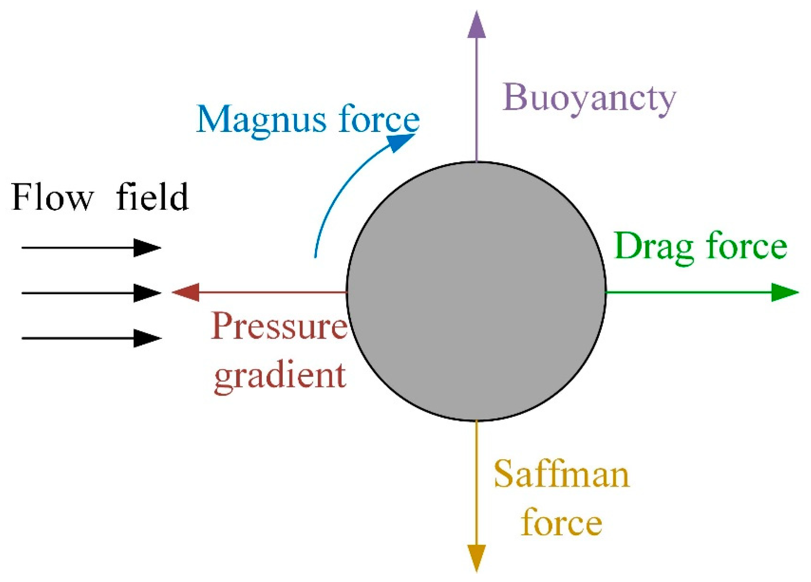
Figure 2.
CFD-DEM coupling calculation flowchart.
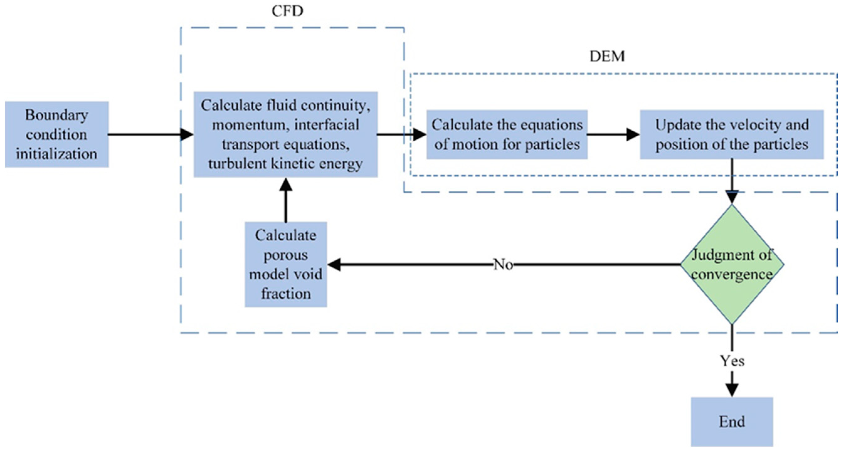
Figure 3.
Schematic diagram of a three-dimensional stirring tank structure. (a) Model structures. (b) Partial structures of upper blades. (c) Particle structures of lower blades.
Figure 3.
Schematic diagram of a three-dimensional stirring tank structure. (a) Model structures. (b) Partial structures of upper blades. (c) Particle structures of lower blades.
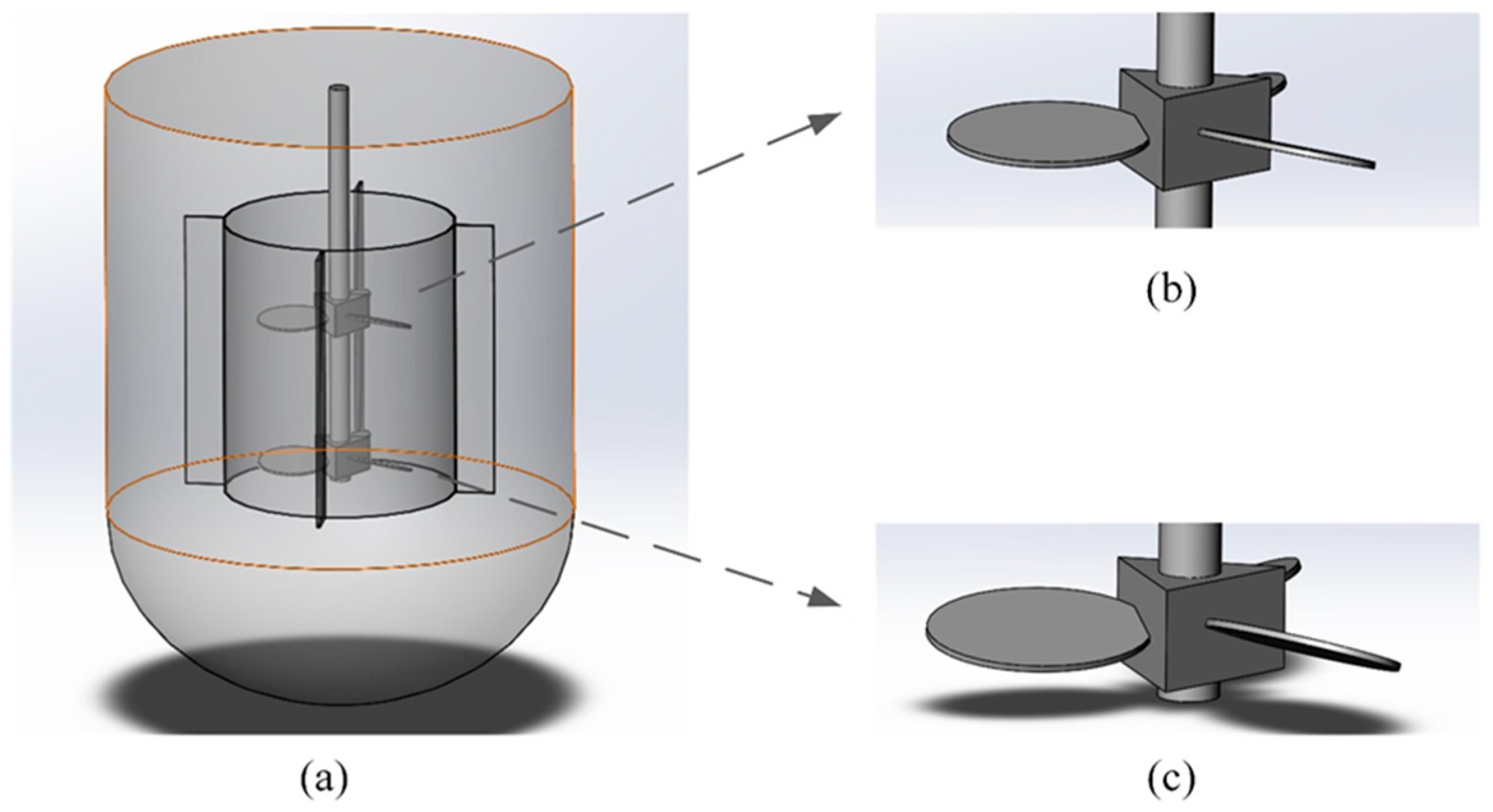
Figure 4.
Grid partitioning of the three-dimensional stirring tank. (a) Overall grid. (b) Overall top view. (c) Local grid refinement near the impellers.
Figure 4.
Grid partitioning of the three-dimensional stirring tank. (a) Overall grid. (b) Overall top view. (c) Local grid refinement near the impellers.

Figure 5.
Average velocity distribution for three different grid quantities.
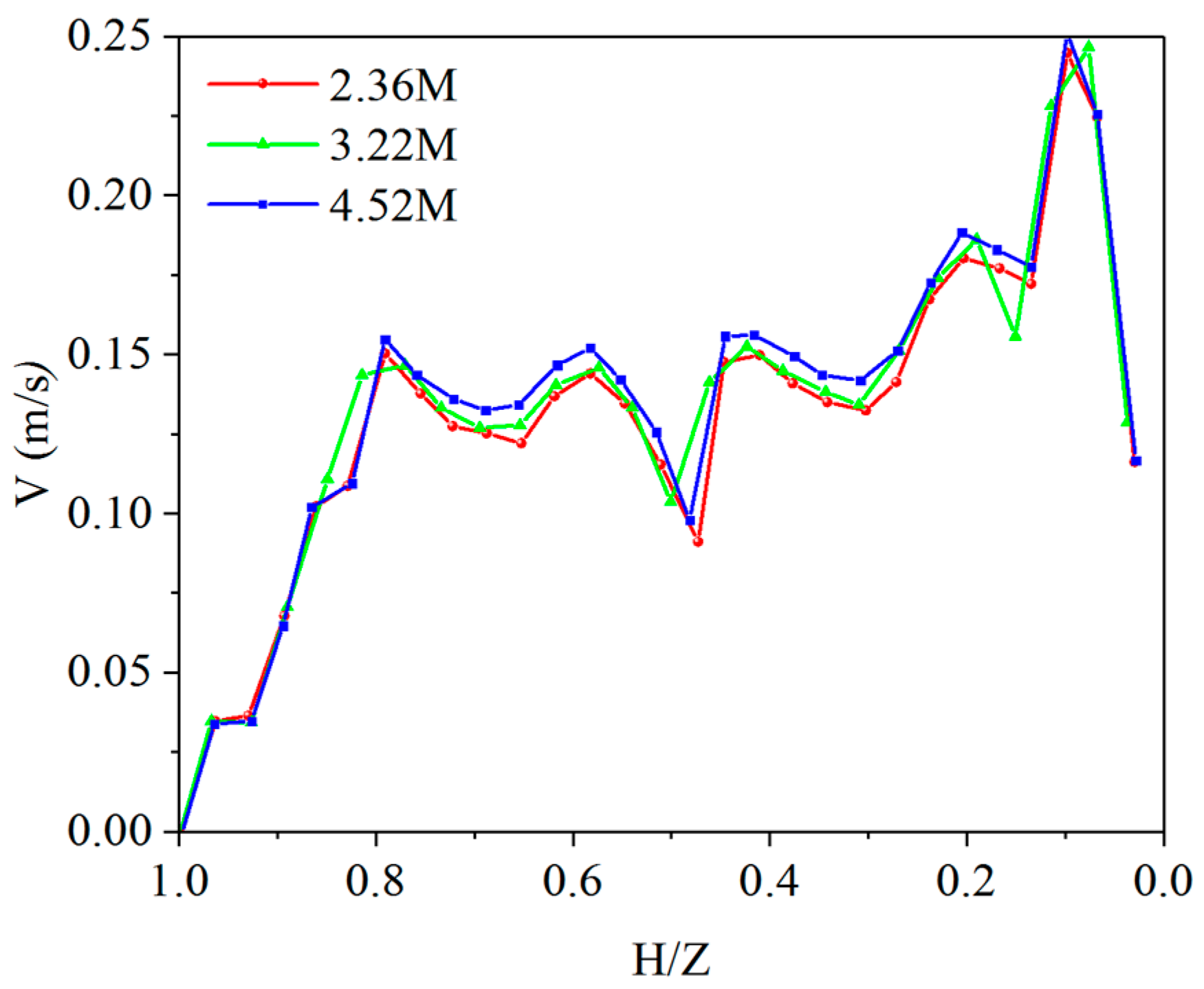
Figure 6.
Impeller velocity cloud diagrams over various times. (a) t = 0.5 s. (b) t = 1.0 s. (c) t = 1.5 s. (d) t = 2.0 s. (e) t = 2.5 s. (f) t = 3.0 s.
Figure 6.
Impeller velocity cloud diagrams over various times. (a) t = 0.5 s. (b) t = 1.0 s. (c) t = 1.5 s. (d) t = 2.0 s. (e) t = 2.5 s. (f) t = 3.0 s.

Figure 7.
Impeller velocity profile over various times. (a) t = 0.5 s. (b) t = 1.0 s. (c) t = 1.5 s. (d) t = 2.0 s. (e) t = 2.5 s. (f) t = 3.0 s.
Figure 7.
Impeller velocity profile over various times. (a) t = 0.5 s. (b) t = 1.0 s. (c) t = 1.5 s. (d) t = 2.0 s. (e) t = 2.5 s. (f) t = 3.0 s.
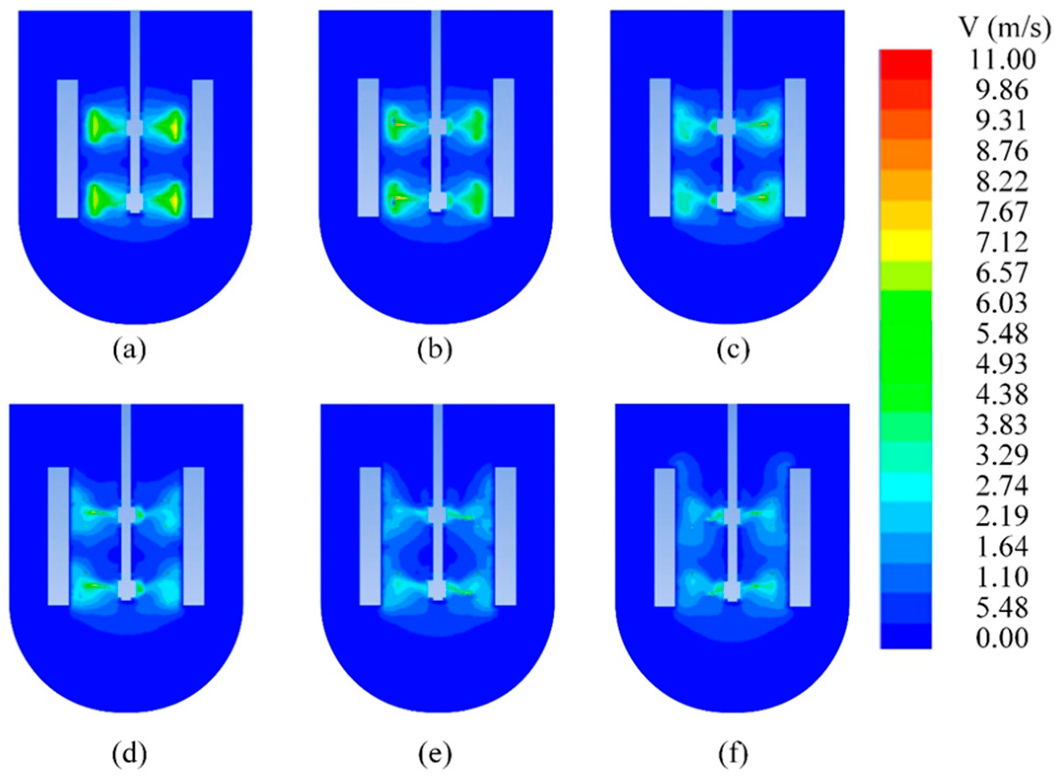
Figure 8.
Circulation flow diagram. (a) Velocity vector diagram. (b) Radial velocity curve.
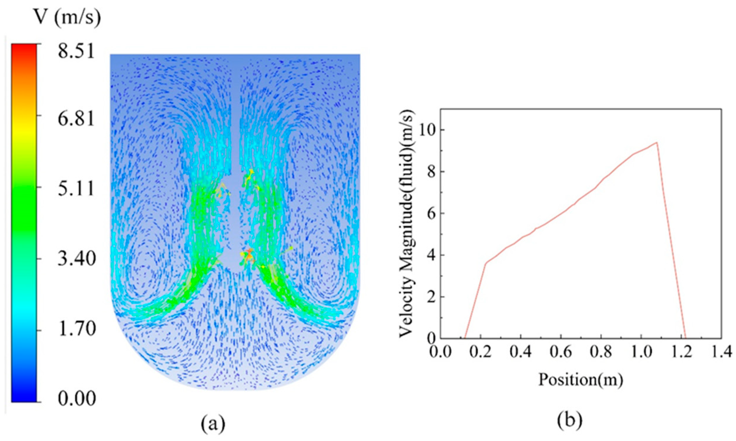
Figure 9.
Pressure load cloud diagrams of upper impellers. (a) t = 1.0 s. (b) t = 2.0 s. (c) t = 3.0 s. (d) t = 4.0 s.
Figure 9.
Pressure load cloud diagrams of upper impellers. (a) t = 1.0 s. (b) t = 2.0 s. (c) t = 3.0 s. (d) t = 4.0 s.
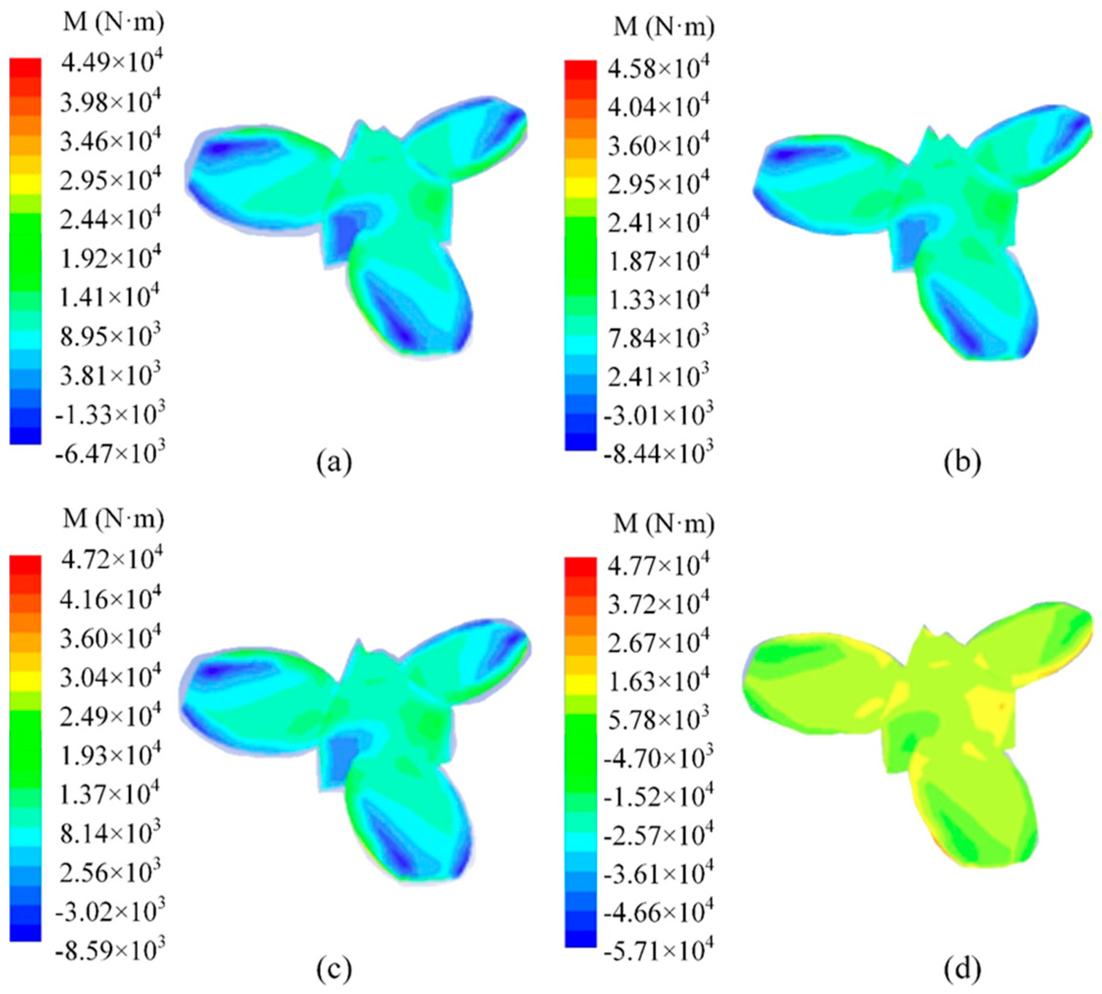
Figure 10.
Pressure load cloud diagrams of lower impellers. (a) t = 1.0 s. (b) t = 2.0 s. (c) t = 3.0 s. (d) t = 4.0 s.
Figure 10.
Pressure load cloud diagrams of lower impellers. (a) t = 1.0 s. (b) t = 2.0 s. (c) t = 3.0 s. (d) t = 4.0 s.
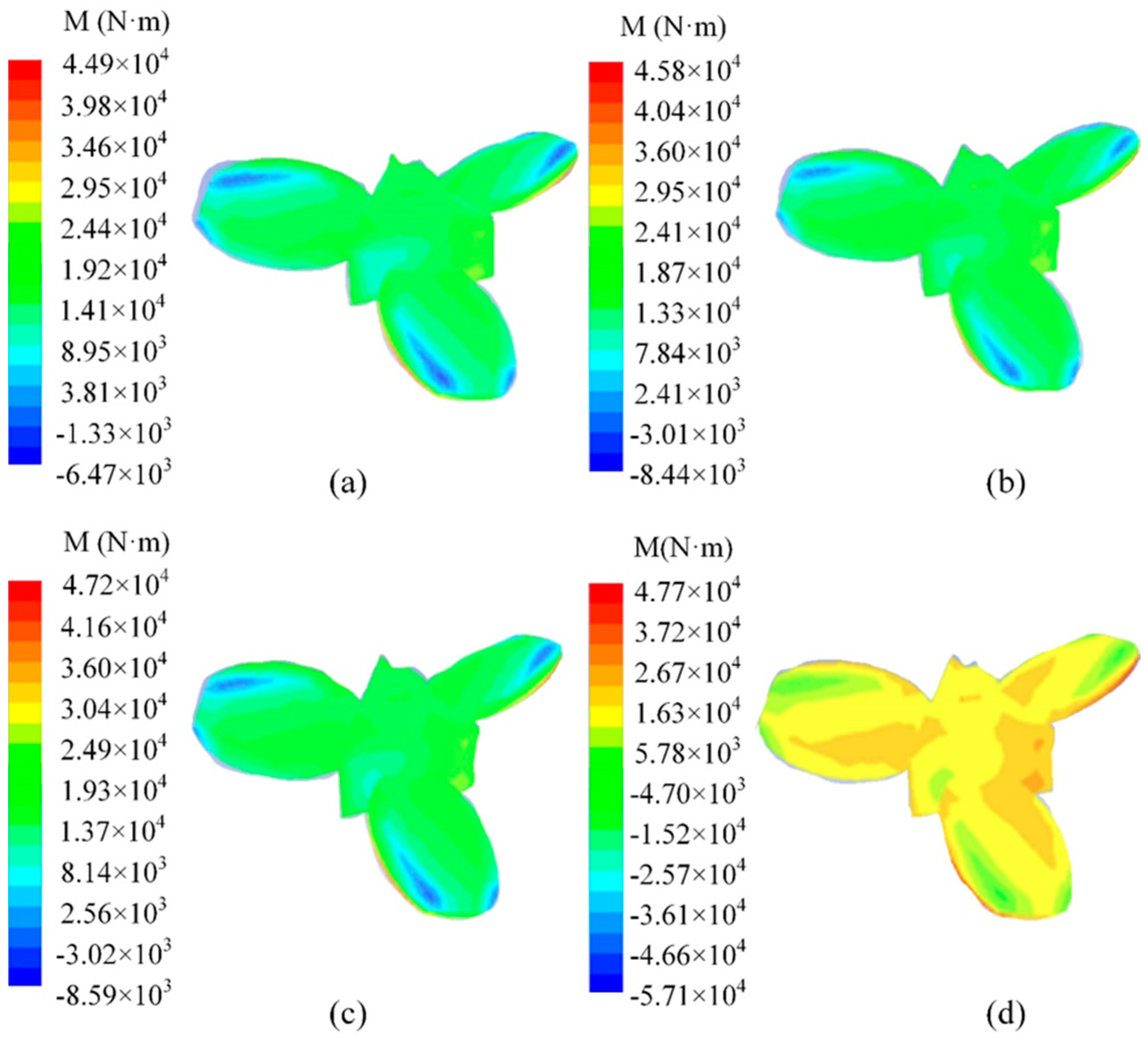
Figure 11.
Power change results of impellers. (a) Upper impeller. (b) Lower impeller.
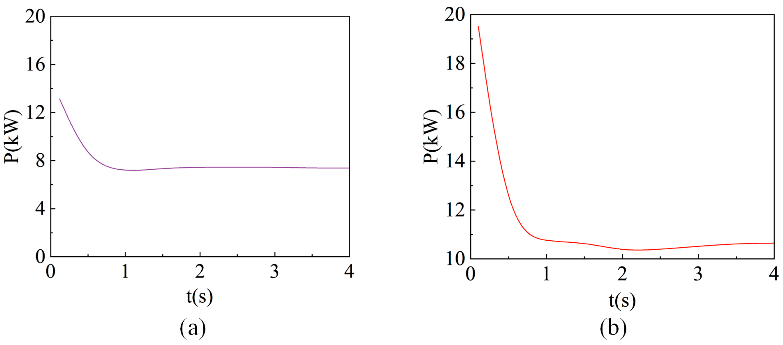
Figure 12.
Velocity evolution patterns of the particle flow. (a) t = 0.5 s. (b) t = 1.0 s. (c) t = 1.5 s. (d) t = 2.0 s. (e) t = 2.5 s. (f) t = 3.0 s.
Figure 12.
Velocity evolution patterns of the particle flow. (a) t = 0.5 s. (b) t = 1.0 s. (c) t = 1.5 s. (d) t = 2.0 s. (e) t = 2.5 s. (f) t = 3.0 s.

Figure 13.
Flow line trace diagrams of the particle flow. (a) t = 0.5 s. (b) t = 1.0 s. (c) t = 1.5 s. (d) t = 2.0 s. (e) t = 2.5 s. (f) t = 3.0 s.
Figure 13.
Flow line trace diagrams of the particle flow. (a) t = 0.5 s. (b) t = 1.0 s. (c) t = 1.5 s. (d) t = 2.0 s. (e) t = 2.5 s. (f) t = 3.0 s.


Table 1.
Variation data of impeller torques.
| Impeller Wheel | Time (s) | Pressure Load (N·m) | Viscosity Force Load (N·m) | Total Moment (N·m) |
|---|---|---|---|---|
| Upper impeller | 0.1 | 504.949 | 19.696 | 524.6456 |
| 0.5 | 301.193 | 15.759 | 316.952 | |
| 1.0 | 269.601 | 14.137 | 283.737 | |
| 1.5 | 279.926 | 13.886 | 293.812 | |
| 2.0 | 286.852 | 13.677 | 300.529 | |
| 2.5 | 285.349 | 13.423 | 298.772 | |
| 3.0 | 284.205 | 13.33 | 297.535 | |
| 3.5 | 282.877 | 13.128 | 296.005 | |
| 4.0 | 280.845 | 12.908 | 293.753 | |
| Lower impeller | 0.1 | 758.362 | 18.906 | 777.268 |
| 0.5 | 430.571 | 14.216 | 444.786 | |
| 1.0 | 418.029 | 10.315 | 428.344 | |
| 1.5 | 419.687 | 8.516 | 428.203 | |
| 2.0 | 404.909 | 8.415 | 413.384 | |
| 2.5 | 407.917 | 8.449 | 416.367 | |
| 3.0 | 412.129 | 8.536 | 420.665 | |
| 3.5 | 416.251 | 8.552 | 424.803 | |
| 4.0 | 418.661 | 8.546 | 427.207 |
Disclaimer/Publisher’s Note: The statements, opinions and data contained in all publications are solely those of the individual author(s) and contributor(s) and not of MDPI and/or the editor(s). MDPI and/or the editor(s) disclaim responsibility for any injury to people or property resulting from any ideas, methods, instructions or products referred to in the content. |
© 2024 by the authors. Licensee MDPI, Basel, Switzerland. This article is an open access article distributed under the terms and conditions of the Creative Commons Attribution (CC BY) license (https://creativecommons.org/licenses/by/4.0/).
Share and Cite
MDPI and ACS Style
Ge, M.; Zheng, G. Fluid–Solid Mixing Transfer Mechanism and Flow Patterns of the Double-Layered Impeller Stirring Tank by the CFD-DEM Method. Energies 2024, 17, 1513. https://doi.org/10.3390/en17071513
AMA Style
Ge M, Zheng G. Fluid–Solid Mixing Transfer Mechanism and Flow Patterns of the Double-Layered Impeller Stirring Tank by the CFD-DEM Method. Energies. 2024; 17(7):1513. https://doi.org/10.3390/en17071513
Chicago/Turabian StyleGe, Man, and Gaoan Zheng. 2024. "Fluid–Solid Mixing Transfer Mechanism and Flow Patterns of the Double-Layered Impeller Stirring Tank by the CFD-DEM Method" Energies 17, no. 7: 1513. https://doi.org/10.3390/en17071513
Note that from the first issue of 2016, this journal uses article numbers instead of page numbers. See further details here.