Abstract
Malaysian wind maps used in wind analysis and engineering design are dated back to the last 50 years of wind data. Cotemporally, the mean wind speed was used as the basic wind design and due to changes in the weather condition worldwide, wind monitoring assumption and structure design are jeopardized. Therefore, this study aims to map the wind based on the trend of the highest wind speed recorded. The wind speed was analyzed based on a trend basis. The study included 42 Malaysian Metrological Department weather stations and the annual wind speed was acquired based on the monthly highest wind speed (1990–2019). The data were then processed using the 95% confidence interval method to determine the mean of the month, and the annual wind trendline was obtained. The trendline was then clustered using Ward’s method with the assistance of the high-level programming language, PYTHON v3.11.6. The clustering analysis produced two clusters for the Malaysian Peninsula and two for Sabah and Sarawak. The recommendation is to use the highest wind speed recorded on the map as the design wind speed. The recommendation is expected to help experts to compensate for the uncertainties in wind speed during the design stage and avoid incidents in the field.
1. Introduction
In the light of complimenting a good definition of design procedures for structures, especially tall buildings and structures such as wind turbines, it is important to consider the dynamic changes and uncertainties in the environment that simulate as loading. This aspect is quite a big challenge for engineers presently. The trend on wind loading estimation and prediction is tuned in adapting the extreme case, whereby the highest value is considered [1,2,3].
Observation and continuous monitoring can update the wind database in aiding engineers to better understand the surroundings before making decisions in the design process. Careful consideration of this matter will ensure public safety and the performance of the built environment with regard to uncertainties in the ever-changing environment.
Wind clustering can reduce the cost of constructing a wind structure such as a wind turbine. Considering the construction of these structures must be effective in terms of the location. Therefore, clustering wind speed is essential for having a cost-effective wind turbine. To further reduce the cost of construction and operating the wind turbine, the elements of development zone, manufacturing zone, ports, and demand can be inserted into the clustering parameters [4].
Wind speed trend analysis has been studied in many papers, either in environmental wind studies or engineering due to wind effects. Wind trend plays a significant role in optimizing the energy produced by the windmill. Kusiak (2010) conducted clustering analysis to predict the power generation output based on the wind speed. The study, however, does not show the wind speed data. Therefore, the power generation prediction from the clustering of wind speed was not accurate [5]. As for environmental aspect studies of wind trends, Angosto (2002) has conducted a prediction on the atmospheric pollution by using wind clustering analysis. The research found five patterns of wind speed in the Cartagena. For example, the first cluster showed that 6.5% of wind directions are north-northwest and north. The second wind direction cluster was comprised of south-southwest and south. The procedure use is hierarchical (average linkage) and non-hierarchical (k-means) [6].
Grouping of annual wind speed patterns is doable if the study area is the same. In 2017, Yesilbudak et al. conducted a clustering analysis for multidimensional wind speed in 75 provinces in Turkey. The clustering method used was the k-means. The analysis found that the cities with constant and high average wind speed are Canakkale and Mardin. These cities are in Cluster 4 and the silhouettes coefficients is 0.5224. The poorly silhouette coefficients are in Cluster 1, which contains Duzee, Amasya, and Siirt, and the silhouette coefficients for this cities are 0.7294, 0.7198, and 0.7111 [7].
Within the scope of this investigation, the research acknowledges the utilization of the k-means algorithm as a segmentation technique in existing literature. The k-means algorithm operates under the assumption that D represents the dataset comprising n observations, and k represents the designated number of clusters. It computes dissimilarity between every pair of observations employing various distance metrics. Specifically, four distinct distance measures are employed: Squared Euclidean, City-Block, Cosine, and Pearson.
To ascertain the most suitable distance measure, the research employs the silhouette coefficient, which ranges from −1 to +1, to evaluate the assignment of observations to clusters. Accuracy is defined based on a higher silhouette coefficient, approaching 1, indicating that an observation is well-suited to its respective cluster. The silhouette coefficient is formally defined as follows in Equation (1).
where, the a(yi) is the average dissimilarity of yi, which is the element of (∈) Sk to all other yj ∈ Sk and b(yi) is the minimum average of dissimilarity of yi ∈ Sk to all other yj ∈ Sl.
The utilization of the k-means algorithm, in conjunction with the silhouette coefficient, yields a more robust clustering solution during the analysis.
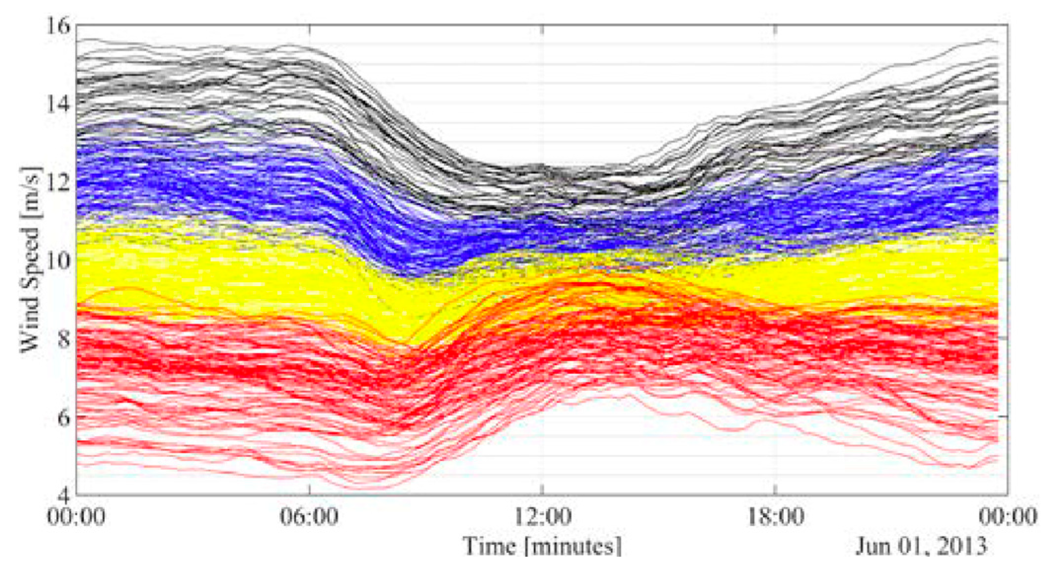
The research by Vuuren et al., 2019, uses the mean wind speed from 2009 until 2013, with the area of study varying from 5263 to 15,214 square kilometers. The research covers an area four times larger than Malaysia. With the numerous data from South Africa, the researchers do not include the detailed wind station where the data were obtained, and the research also includes the time of use tariff into the clustering for user demand for energy cost. Therefore, the mean daily wind speed is only evaluated during the high-demand session using multiple methods of clustering including k-means and Wards method. As shown in Figure 1, the mean daily wind speed was presented according to cluster in the high-demand season [8].

Figure 1.
Mean daily wind speed profiles associated with the individual cluster for the high demand season [8].
Research conducted by Clifton in 2012, demonstrates the utility of k-means clustering. The research identifies the relationships between the wind speed at turbine height and climate oscillations. The research uses fourteen years of data from one 80 m tower at the National Wind Technology Center (NWTC), Colorado. The wind speed is clustered by four dominant flows using k-means clustering. The aim of this research, however, focuses on the stable wind speed by clustering the zonal wind speed and meridional wind speed. It shows that most of the stable wind is located at the zonal area. The research focuses on the direction and the speed of the wind to ensure that the wind turbine is working efficiently. Therefore, the highest wind speed recorded in the research was not highlighted. The findings of the research are shown in Figure 2 below [9].
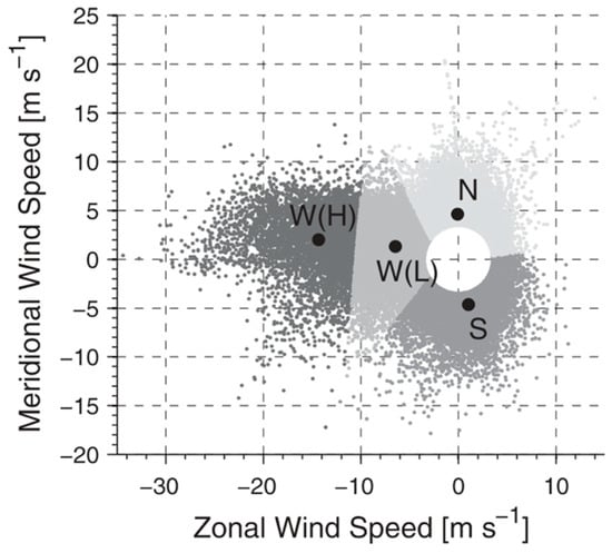
Figure 2.
Optimal wind cluster at 80 m at the NWTC near Boulder [9].
Multiple incidents have occurred regarding lattice structure, especially communication infrastructure in Malaysia. Between 2020 and 2022, it has been reported that four communication lattice structures failed due to wind action, as reported by Malaysian Communication and Multimedia Commissions (MCMC). The failed lattice structures ranged from 30 to 75 m in height. The latest failure was located at Kampung Gelong Badak, Kelantan, where on 22 July 2021, a 75 m three-legged communication tower collapsed. In the report, MCMC stated that the failure was due to the strong wind [10].
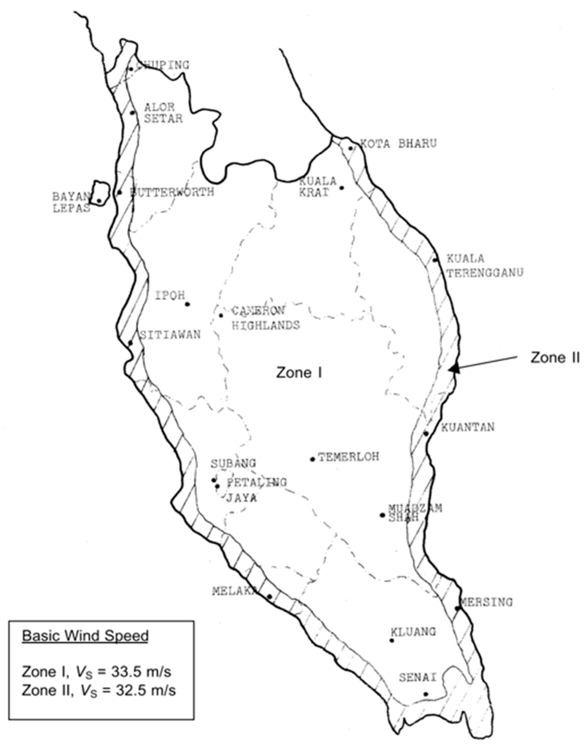
Malaysian structure design adopts the Malaysian Standard Code of Practice on Wind Loading for Building Structure, 2002, developed by the Department of Standard Malaysia. In the code, the wind speed recommended is differentiated based on the geographical aspect. The code suggests that the wind loading should be the same throughout the coastline (Zone 2) of the Malaysian Peninsula and remain the same throughout the mainland (Zone 1) in Figure 3 below [11].

Figure 3.
Basic wind speed for Peninsular Malaysia [11].
The Indonesian Wind Code applies a much lower basic design mean hourly wind speed than the Malaysian code. The code applies the basic design wind speed of 20 m/s at the height of 10 m and 25 m/s for sites located at coastal lines of Indonesia [12].
The data obtained from the Malaysian Metrological Department show similar results in wind speed distribution in the Malaysian peninsula. The data show that the inland wind speed is much higher than the peninsula’s coastal area. For example, the wind speed in the inland of the peninsula reached 39 m/s in Ipoh, Perak, compared to the highest coastal windspeed of 35.6 m/s in Mersing, Johor. The result is also similar in Sabah and Sarawak, where the maximum wind speed observed in the inland area is higher compared to coastal areas. The Kuching wind station in 1992 showed a higher speed than the other station in Malaysia. The station has shown a speed of 41.7 m/s, equivalent to 150 km/h of wind speed.
Therefore, the research intention is to determine whether there is any pattern of maximum wind speed for the last 30 years, which can help the designers further understand wind behavior in Malaysia. Furthermore, pattern observation can also help to cluster similar patterns of wind speeds according to their localities through mapping for Peninsular Malaysia and Borneo (Sabah and Sarawak).
2. Methodology
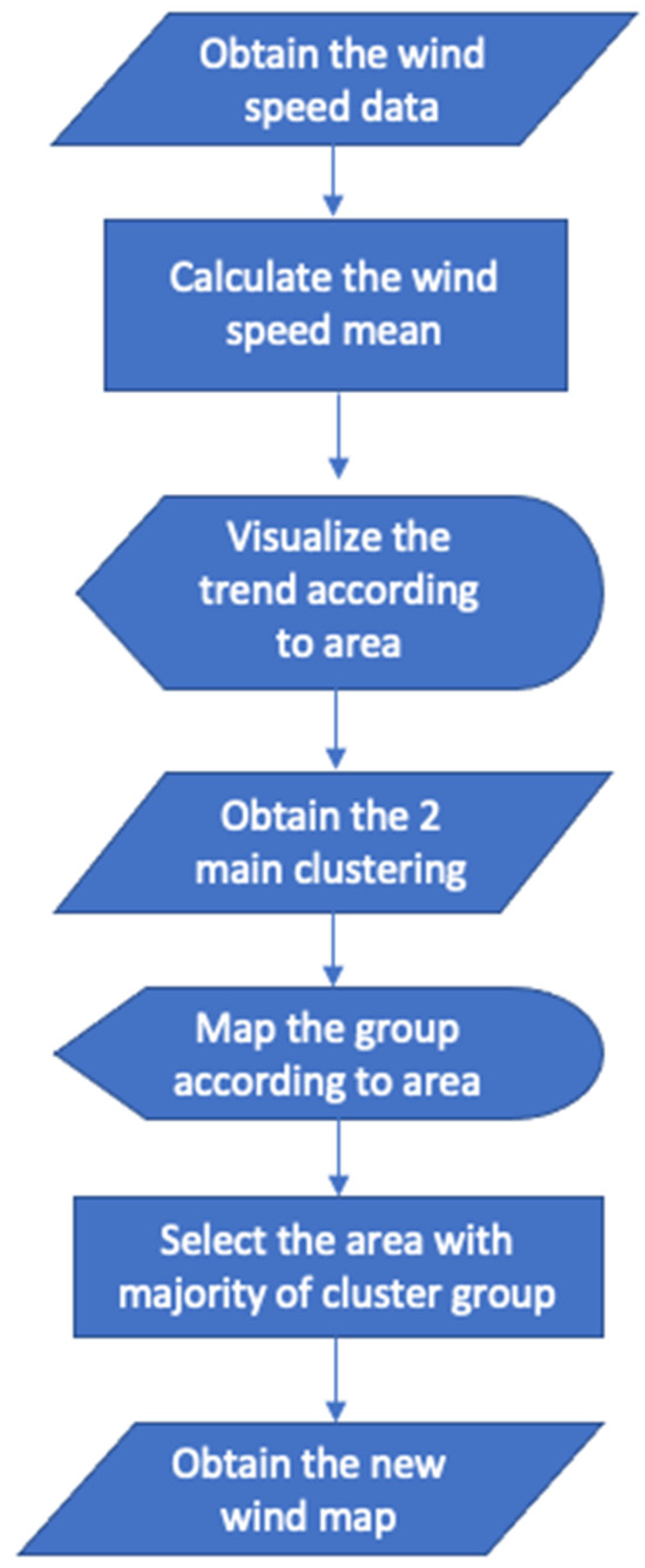
The research method focuses on wind data analysis with mapping. The analysis shall be conducted with 3 major software: Excel v16.78, PYTHON v3.11.6, and QGIS v3.16. Figure 4 below shows the flowchart of wind analysis conducted to create a new mapping for Peninsular Malaysia and Borneo. Compared to the original Malaysian Standard Code of Practice for Wind Loading 2002, the research method analysis aims to create a map for the peninsula and the Borneo region.

Figure 4.
Flowchart of wind mapping.
2.1. Wind Data Collection
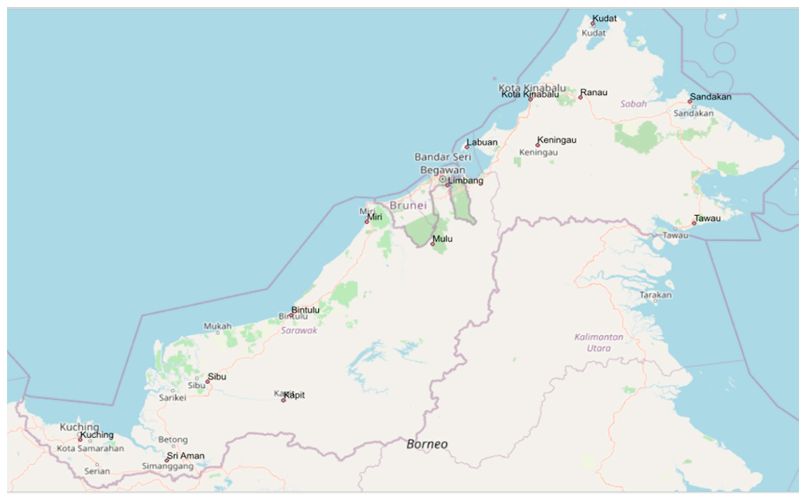
The wind speed data are obtained from the Malaysian Metrological Department (MET). The wind speed is obtained in meters per second unit (m/s). Maximum wind speed data were collected from 42 weather stations in Malaysia from the year 1990 to 2019, including twenty-seven stations in Semenanjung as in Figure 5, seven stations in Sabah, and eight stations in Sarawak as shown in Figure 6. The list of wind stations is in Table 1 below.
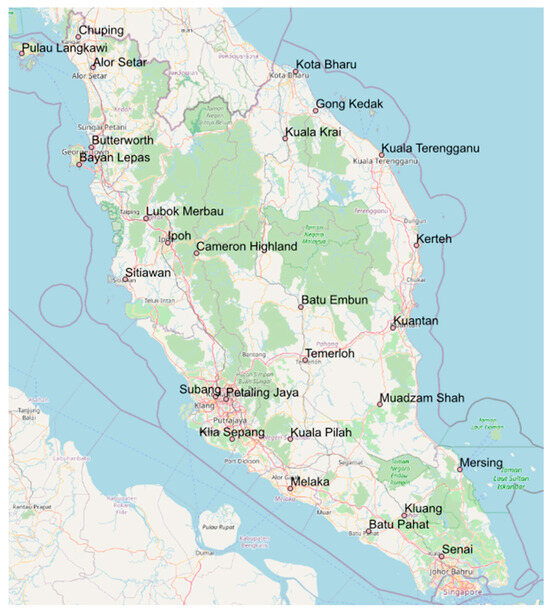
Figure 5.
Wind station in Semenanjung.
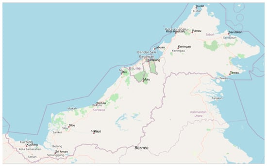
Figure 6.
Wind station in Sabah and Sarawak (Borneo).

Table 1.
List of wind stations.
2.1.1. Data Collection Procedure
Wind data were collected at the above wind station situated at various locations of Malaysia. The data obtained was specifically the highest wind speed recorded in a month. The data obtained from MET included the direction of wind. However, the direction of wind is not considered in this research due to the scope of the research objective, which only requires the highest wind analysis. The wind data are acquired by using the MET Wind Vane and Anemometers cup (Figure 7) located at all 42 wind stations. Wind vanes collected the direction and the wind speed. The wind direction was measured according to the northern direction clockwise. The wind speed was recorded via the use of the Anemometers cup, which consists of three hemispheric cups. The cup captured differences in wind pressure, as well as what caused it to rotate, which were collected as wind speed. The wind speed was recorded in meter per second (m/s) or knots.

Figure 7.
Wind Vane (right) and Anemometers cup (left).
2.1.2. Sample of Wind Data
Monthly data obtain from 42 wind stations constitute 20 years of monthly data. Table 2 below shows the data obtained by Kuching wind station in Sarawak, Malaysia. The green color indicates the highest wind data that were required in this study. The red data show the slower wind blow during observation. It is observed that from the month of June until October, the wind trend is high and becomes slower from November until May. These are the trends that were observed during the study.
Table 2.
Monthly maximum wind speed data of Kuching wind station.
Table 3 below shows the sample of data taken from Bayan Lepas wind station in Pulau Pinang, Malaysia. The data show that the windiest month in this station was in August. The trend shows that the windiest month started in the month of July until October. The wind speed started to slow in the month of November and continues to June. This shows that compared to Kuching wind station, the Bayan Lepas wind station is windier. However, the sudden blow of wind in the Kuching area is higher compared to the windier area of Bayan Lepas.
Table 3.
Monthly maximum wind speed data of Bayan Lepas wind station.
2.1.3. Credibility of Data
The wind speed data were provided by MET Malaysia. The data observation and data collection of MET Malaysia was conducted in accordance with the World Meteorological Organization (WMO) standard and recommended practices. WMO is the international standardization organization leading in the field of meteorology, hydrology, and related environmental disciplines.
WMO Technical Regulation is an international framework for standardization and intermobility of multiple meteorological aspects. The international framework includes standards and recommendations of practices and procedures mandated by the World Meteorological Congress for adoption by all members. The regulation is responsible for making observations, data exchange, data management forecasting, scientific assessment, and product production for meteorological purpose standardization across WMO member states and member territories. The WMO Technical Regulation is based on the requirement and designed to encourage efficiency and interoperability and support a policy of decision making in disaster risk management, agriculture, aviation, shipping, water management and health [13].
2.2. The 95% Confidence Interval for Mean Data
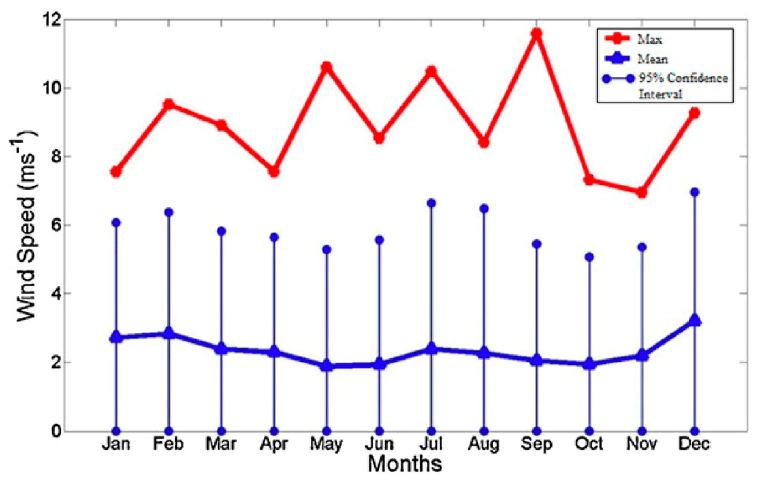
To obtain the monthly mean wind speed of each wind station, the study uses a 95% confidence interval method to obtain each station’s mean of each month. The confidence interval is a method of estimating the mean of the observed data. Tiang and Ishak (2012) studied the wind speed in the measurement site of Bayan Lepas, Pulau Pinang, from January to December 2008. The study uses a 95% confidence interval method to obtain the mean monthly and maximum wind speeds for one year [14]. The data obtained from the 2012 research is as per Figure 8 below.
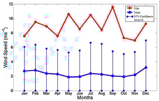
Figure 8.
Mean monthly and maximum wind speed with 95% confidence interval [14].
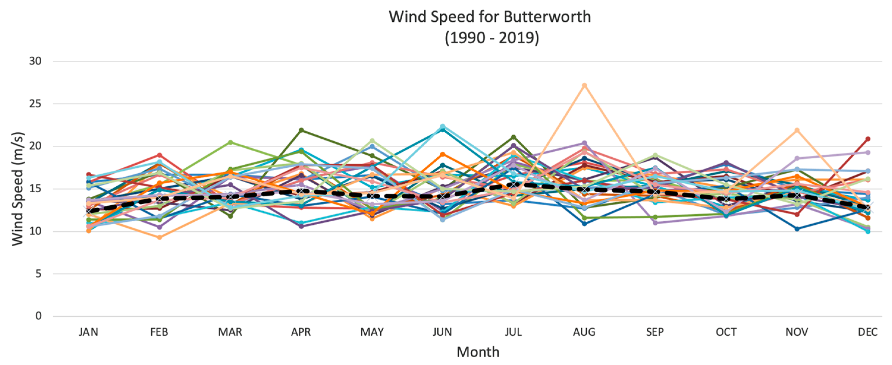
In this study, the 30 years of wind data, starting from 1990 and ending in 2019, are used. Therefore, the estimation of the mean is needed to find the wind trend in the wind station, as shown in Figure 9 below. The sample data were taken from Butterworth Station, Pulau Pinang. The colored line in the figure showing the yearly mean wind speed in Butterworth, Pulau Pinang.
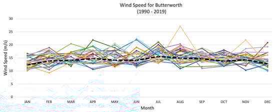
Figure 9.
Sample of wind speed analysis of Butterworth wind station.
The calculation using a 95% confidence interval is a method to determine the mean wind speed. Therefore, the study data contain 30 years of monthly data from January to December. The wind speed varies each year. Therefore, using the confidence interval method, the study can confirm that 95% of the monthly data are the actual mean. Research in 2018 on wind power interval forecasting stated that using the confidence interval method has effectively shortened the interval length [15].
As shown in Equation (2) above, σ is the standard deviation of the data, which measures how to spread the data. xi is the individual wind speed values at a specific wind speed station, and μ is the mean of the wind speed data of the particular year. N is the number of years recording for the station.
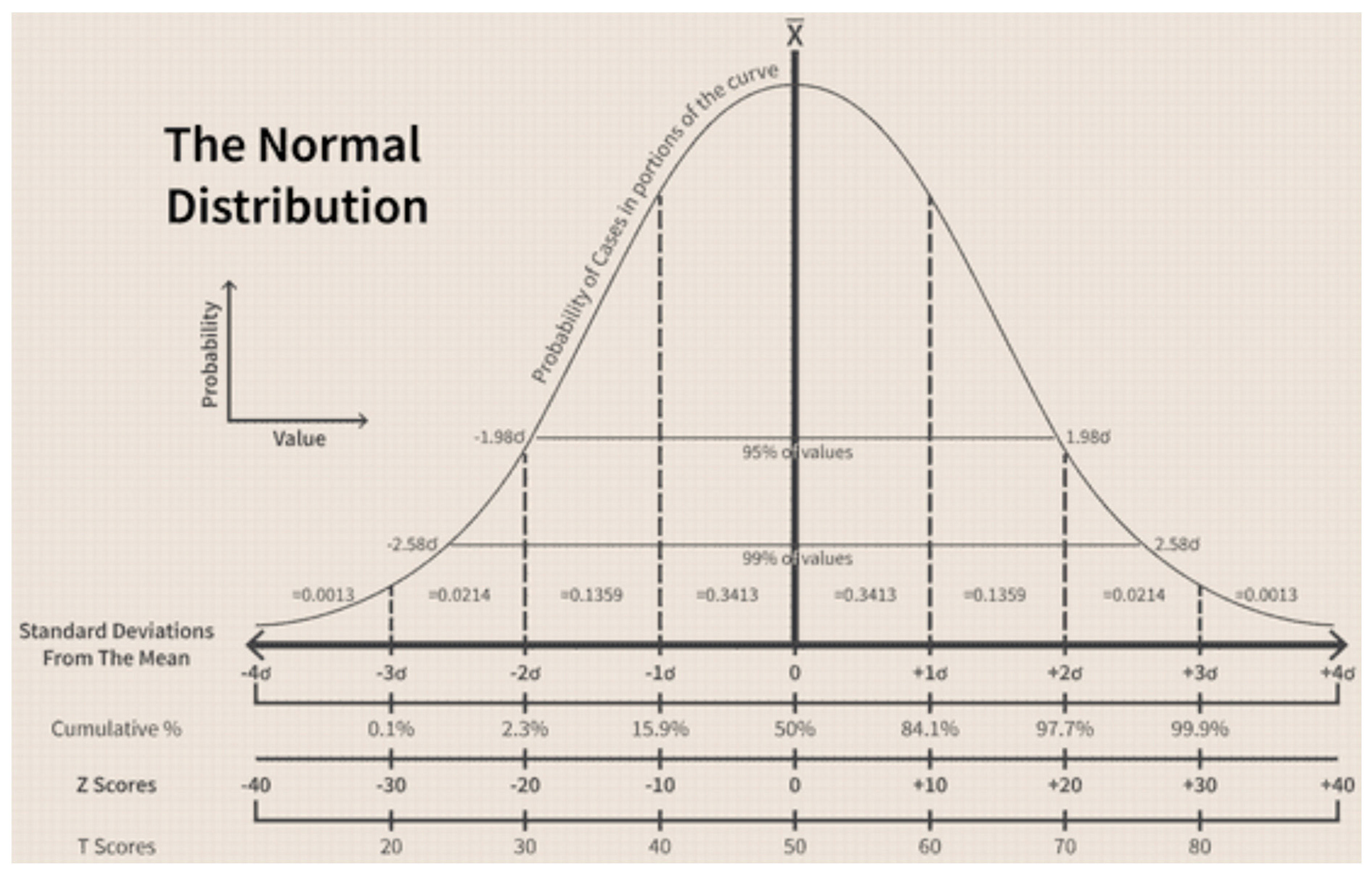
As mentioned above, Figure 10 shows the critical value of z was calculated using the bell curve, which describes a graphical depiction of a normal probability distribution. The curve is shaped based on the standard deviation of the mean [16]. Therefore, the mean data of the stations were plotted together to see the overall trend of the wind surrounding Malaysia.
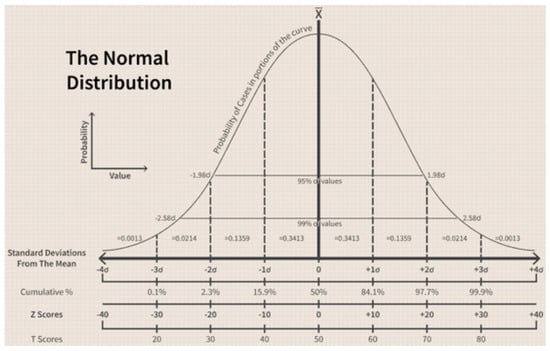
Figure 10.
Plot of normal distribution [16].
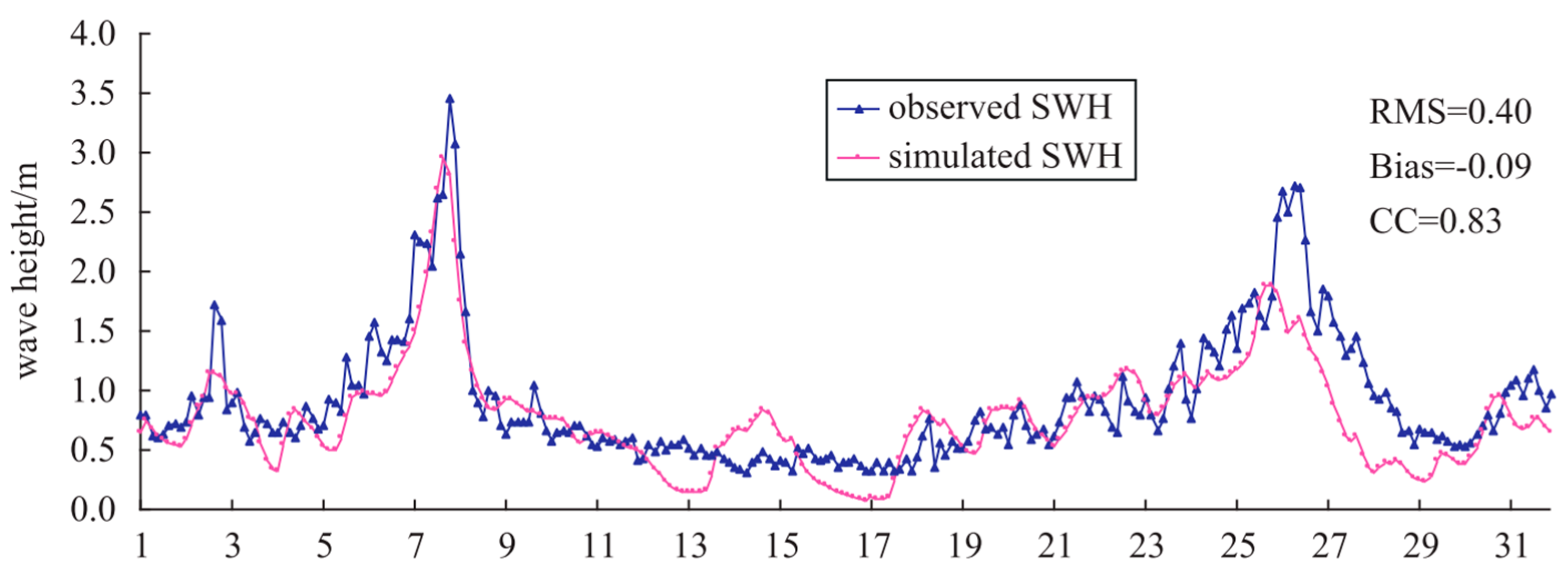
A similar method was used by Chong et al., in 2009 to validate wave data. The researcher used Root Mean Square (RMS) error, bias and correlation (CC). Figure 11 below shows the sample of simulation and observed significant wave height (SWH) of Sata Cape, Japan, in October 2009 [17].
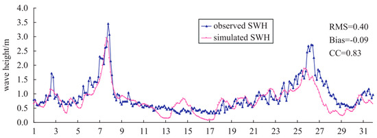
Figure 11.
Simulated SWH and observe SWH in Sata Cape, Japan [17].
The simulation of SWH in Figure 11 shows the observed SWH is slightly bigger than the simulated SWH. This shows that the method has high precision and passes the reliability test.
All calculations for the mean are performed in Microsoft Excel. The selection of Microsoft Excel was due its capability to calculate and readiness in data analysis tools. The calculation also needed to be translated into a graph, which is available in Excel for visualization and observation purposes. Table 4 below shows a sample of the result of the 95% confidence interval for Ipoh wind station.
Table 4.
Monthly maximum wind speed data and 95% confidence level of Ipoh wind station.
2.3. Time-Series Clustering
Time series are variable values ordered by time. In this study, the value provided was wind speed in meters per second with time ordered by monthly data of 30 years. These data are analyzed using various statistical methods such as classification, clustering, and anomaly detection [18].
The clustering of the data shall be made by using machine learning or the high-level programming language “PYTHON”. Clustering is a well-known unsupervised machine learning method for dividing data points into groups called clusters. The observation within the same cluster tends to be more similar than others in a different cluster [19].
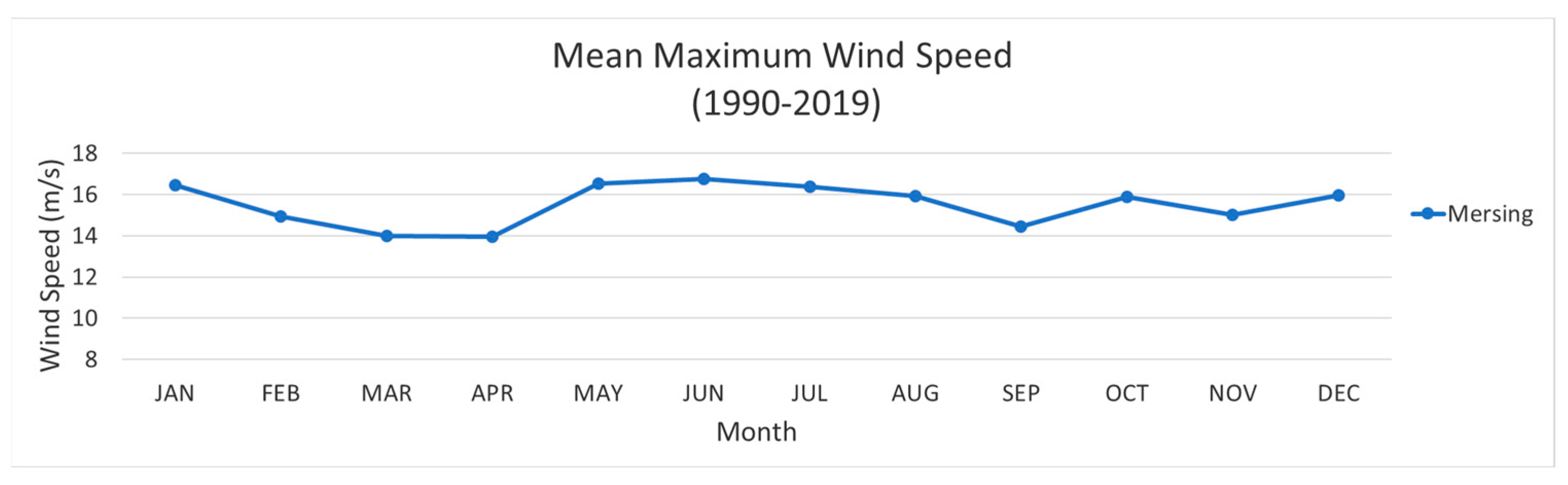
The usage of PYTHON to cluster the time series saves computing and calculation time. The series are converted into individual wind speed time series according to stations. Figure 12 below shows the single line of mean maximum wind speed located at Mersing, Johor. The monthly mean wind speed was calculated earlier with a 95% confidence interval for mean data.
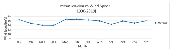
Figure 12.
Single line of mean maximum wind speed located at Mersing wind station.
PYTHON allow the usage of the calculation Wards clustering method into its programming algorithm based using Microsoft Excel data. The mean wind data were consolidated according to location which in the research area, Peninsula Malaysia, and Borneo.
2.3.1. Linkage-Ward Clustering Method
In the investigation conducted in 2018 at Khaaf, Iran, probabilistic wind speed clustering was employed [20]. Azizi’s study utilized the Linkage-Ward clustering technique to categorize wind speed patterns in the region. The research findings indicated that the Ward clustering method outperformed the K-means method in terms of accuracy, albeit with a higher degree of complexity. Over a two-year period, wind speed data collected at 60 min intervals from various wind stations located around Binalood, Iran, were used in the analysis. These wind stations exhibited variations in terms of height, soil composition, and proximity to residential areas. The primary objective of the study was to identify an optimal site for installing a wind turbine in the Binalood region. Consequently, the research concentrated on identifying the windiest areas, a facet that bears relevance to the current study. Notably, the choice of employing the Linkage-Ward clustering method, as opposed to K-means, also came with an increased computational workload.
The investigation determined that the Linkage-Ward clustering method emerged as the prevalent and accurate choice for the study. This method computed dissimilarity between clusters by considering the centroid of each cluster, as depicted in Equation (3).
where dik, djk, dij is the pairwise distance between the cluster i and k, j and k and i and j. i, j, k is the index of cluster. ni, nj, nk is the number of members within cluster i, j and k, respectively.
where a and b are defined as (4), and c = 0 in the Linkage-Ward clustering method.
The clusters that have the lowest increase in cost function (2) are combined. The Ward method used the objective function in the sum of squares from the points to the centroid of the clusters. Figure 13 below shows the Linkage-Ward clustering step by step algorithm.
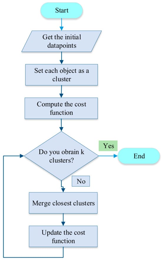
Figure 13.
Linkage-Ward clustering step by step algorithm [20].
The calculation above will result in the lowest increase in the cost function of (2) and combined. The method uses the objective function in the sum of the square from the points to the centroid of the clusters.
2.3.2. Hierarchical Clustering
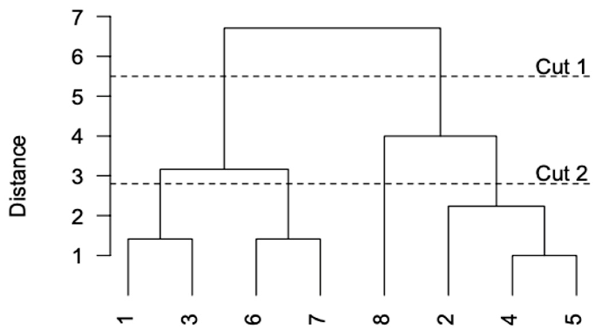
The clustering of wind trends uses hierarchical clustering, which obtains clustering by building a hierarchy of clusters. The cluster was organized as a tree and visualized as a dendrogram, as shown in Figure 14 below.
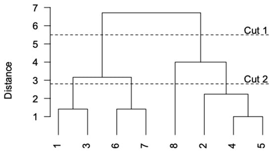
Figure 14.
Hierarchical clustering dendrogram [21].
There are two types of hierarchical clustering, agglomerative and divisive. The agglomerative, which is the Ward’s method that will be used in this research, is the bottom-up approach method, which starts with observation as an individual cluster and, at each step, merges with the closest pair of its cluster. For this research, agglomerative research is more suitable where the observation of each wind station trendline was observed and followed by paring the closest pair of its cluster. The observation of the trendline was conducted earlier in the section above and clustered together with similar trendlines [21].
2.4. Mapping of Wind Speed
Following the clustering outcomes, the study leveraged the Quantum Geographic Information System (QGIS) v3.16, an open-source Geographic Information System (GIS) software developed collaboratively by volunteers and contributors. QGIS is a versatile desktop geographic information system application that offers support for various geospatial tasks, including viewing, editing, printing, and analyzing geospatial data, and it is compatible with multiple platforms. Clusters produced in the last step will be marked as groups in the QGIS maps. Based on the clusters that dominate the area, the area will be marked as one area and use the same highest wind speed in the cluster. The detail of the mapping will be explained in the section below.
3. Result and Discussion
3.1. Overall Mean Maximum Wind Speed
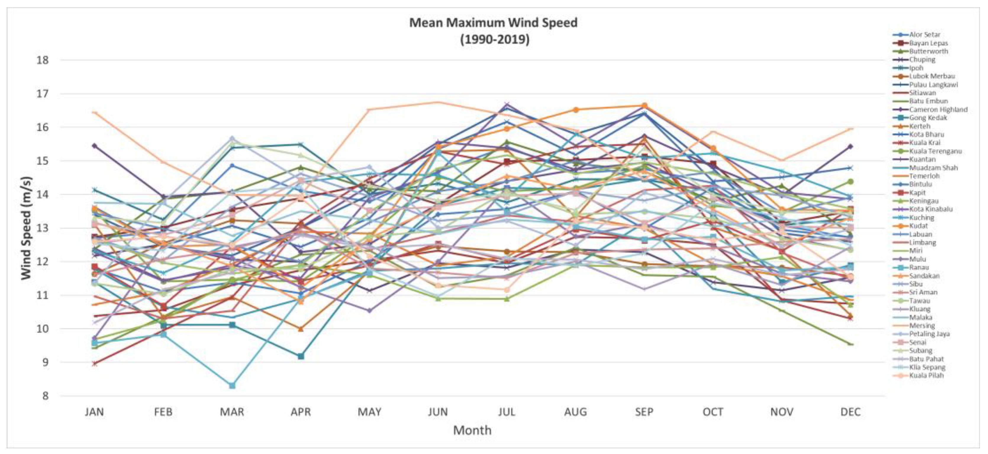
The analysis conducted earlier has confirmed the hypothesis made earlier. The result shows the significant relation between the wind trend surrounding Malaysia. It is also observed that the overall maximum wind trend in Malaysia is almost similar, as shown in Figure 15 below.
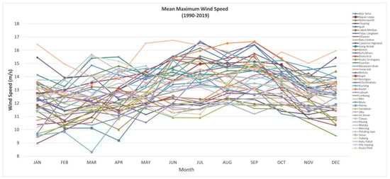
Figure 15.
Overall mean maximum wind speed (1990–2019).
The overall 30 years data also show the similarity in trends. The yearly trend shows that the wind started to increase its speed in the southwest monsoon in May and decreased in September when the northeast monsoon started. The decrease in wind speed before the monsoon may result from positive values of upwelling during the northeast monsoon [22].
It is also found that the mean wind speed between January and February was the time when the wind is at the slowest point. The research confirmed the data by Kok above that between January and February, the overall wind speed in the peninsula is at the slowest point during the transition period of northeast monsoon to southeast monsoon [22].
3.2. Clustering Analysis for Peninsula
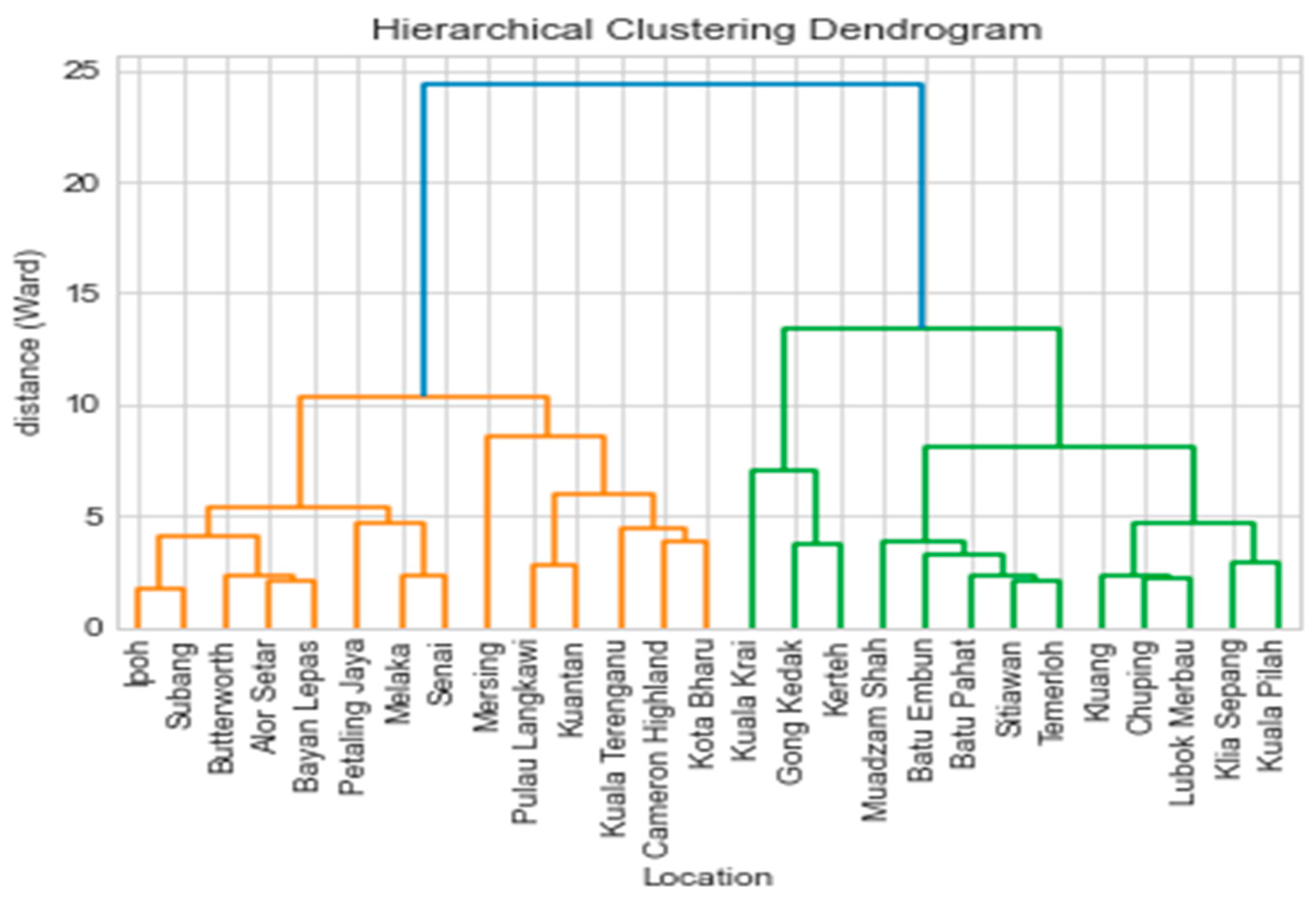
The analysis using the Ward’s method using PYTHON’s programming languages was conducted according to the highest wind speed trends of the station. The result shows that the trend can be grouped in Figure 16 for the Semenanjung dendrogram below.
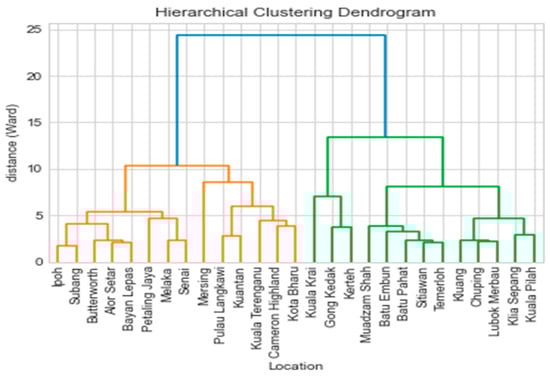
Figure 16.
Hierarchical clustering dendrogram for Semenanjung.
It is found that the clustering analysis using PYTHON programming was successful. The programming was able to cluster the maximum wind trend for all 42 wind stations. The clustering analysis was divided into two areas, Semenanjung and Borneo. The first group mark in orange line in Figure 16 consists of 13 wind stations that have shared a similar wind trend for 30 years. The cluster’s highest recorded wind speed was 39 m/s in March 1990 at the Ipoh wind station. However, the overall wind speed exceeds the Malaysian Standard of wind loading of 33.5 m/s. Three of the wind stations show that the speed is higher than the Malaysian standard. The three wind stations are Ipoh, Mersing, and Kota Bharu, where the readings were 39 m/s, 36.5 m/s, and 34.8 m/s.
Two of the stations were Mersing and Kota Baharu, located at the shore of the South China Sea and facing the northeast monsoon occasionally occurring from November to March. Therefore, the recommendation of slower wind speed in the South China Sea coastal area was not suitable since the northeast monsoon is usually known to bring heavy rain to the peninsula, especially to the eastern peninsula of Malaysia. The Ipoh wind station also shows a similar trend in 1990, where the highest recorded wind speed was happening in March when the transition period of the Northeast monsoon was happening. As the Ipoh wind station is located at the vast plane of Ipoh, where any obstruction whether natural or man-made does not obstruct the area, the transition usually carries uncertainty as to whether it blows to the area, which causes the wind speed to increase during the period.
However, the second cluster shows a slower wind speed where the highest recorded wind speed of the cluster is in Temerloh, where the wind speed recorded was 27 m/s, which is below the Malaysian standard for wind loading. The cluster, however, shows an overall slower speed than the first cluster, with an overall speed that is slower than the Malaysian standard. However, the slower wind speed should not be neglected since two of the stations, Temerloh and Gong Kedak, where the highest wind speed recorded is 27.2 m/s and 26.2 m/s, respectively, are in zone 1 of the Malaysian Standard of wind loading.
3.3. Mapping of Peninsula Malaysia
Mapping of the peninsula was conducted on QGIS software. The markers indicating the clusters produced earlier by the Wards method of clustering was placed on the map to illustrate the dominant cluster in the area. The research sees the domination of certain clusters in the area show the similarity in wind trend. Therefore, by using QGIS software, the markers were place as per below Figure 17.
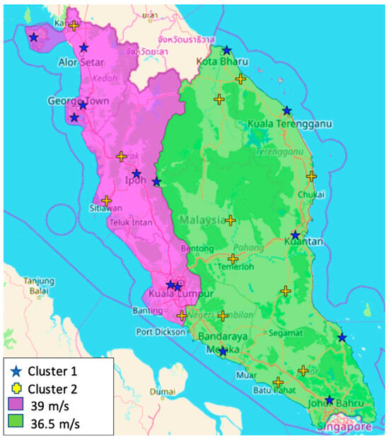
Figure 17.
Wind zoning of Semenanjung.
Based on the majority of Cluster 1 located at the north and west of peninsula Malaysia, the research suggests that the area from Perlis, Kedah, Pulau Pinang, Perak, Selangor and Kuala Lumpur are grouped and marked in purple color. The second area is where the majority of Cluster 2 are marked in green color. The area consists of Kelantan, Terengganu, Pahang, Negeri Sembilan, Melaka, and Johor.
The research also suggests the basic wind speeds (Vs) distribution map as per Figure 17 above. The significance of the map is that it has been developed according to the 30 years’ trend of maximum wind. The mapping of the trend also helps designers and wind experts to further understand the behavior of the wind in the peninsula of Malaysia. The understanding of wind behavior is important to the designers so the design can withstand the highest wind possible compared to the current method, where the designers are only allowed to follow the basic wind speed. The condition has resulted in the design being underestimated, where many of the structures, especially small poles and higher structures, failed during high-speed wind situations.
Table 5 shows the clustering detail for Cluster 1 in Semenanjung. The cluster consists of 13 wind stations, which share similar wind trends for 30 years. The highest recorded wind speed for this cluster was 39 m/s in March 1990 at the Ipoh wind station.
Table 5.
Clustering detail for Cluster 1 Semenanjung.
3.4. Clustering Analysis for Borneo
The Borneo analysis comprises 15 wind stations located throughout the Borneo region. The stations were located in both coastal and in hilly areas of central Borneo. As for the coastal area of Borneo, the west coast faces the South China Sea while the east coast meets the Sulu Sea. The east coast contains three stations: Tawau wind station, Sandakan wind station and Kudat wind station. However, these stations are more prone to the yearly tropical cyclones that devastate the area of the Philippines and the east coast of Sabah.
The analysis with PYTHON has successfully clustered all 15 sites into two main clusters. The trend-based analysis has equally divided the station into two clusters as shown in the hierarchical clustering dendrogram in Figure 18 below.
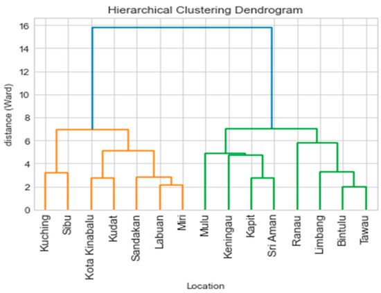
Figure 18.
Hierarchical clustering dendrogram for Borneo.
The analysis has successfully created two main clusters for the Borneo province. The first cluster mainly contains the wind station with a higher wind speed. The first sub-cluster for cluster 1 highlighted in orange in Figure 18 includes the highest ever recorded wind speed in Malaysia. The first wind station is the Kuching wind station, which has the highest recorded wind speed in Malaysia, 41.7 m/s in 1992. The same sub-cluster contains the second highest wind speed recorded at 38.6 at Sibu Wind Station in 2015. The first cluster has shown that the Malaysian Standard of Wind Loading recommendation is lower than what is happening in the area. This is due to the location of Borneo Island itself, which is closer to the Pacific Ocean and much more prone to a tropical cyclone.
The second sub-cluster of Cluster 1 also showed a higher wind speed compared to the Malaysian Standard. Two of the wind stations show a higher speed compared to the Malaysian Standard wind speed. Kudat Wind Station experienced a 34.5 m/s wind speed in 2002, which is higher than the Malaysian Standard, and Kota Kinabalu Wind Station has experienced a 33.1 m/s wind speed. Considering wind is one of the unpredictable elements in the design, the designer should be more wary of the possibility of higher wind speeds hitting the designed structure.
Table 6 shows the clustering detail for Cluster 1 in Borneo. The cluster consists of seven wind stations, which share similar wind trends. The location of the site is also similar, where the majority of the site is located at the coastal area of Borneo. The highest recorded wind speed for this cluster was 41.7 m/s in 1993 at the Kuching wind station.
Table 6.
Clustering detail for Cluster 1.
3.5. Mapping of Borneo
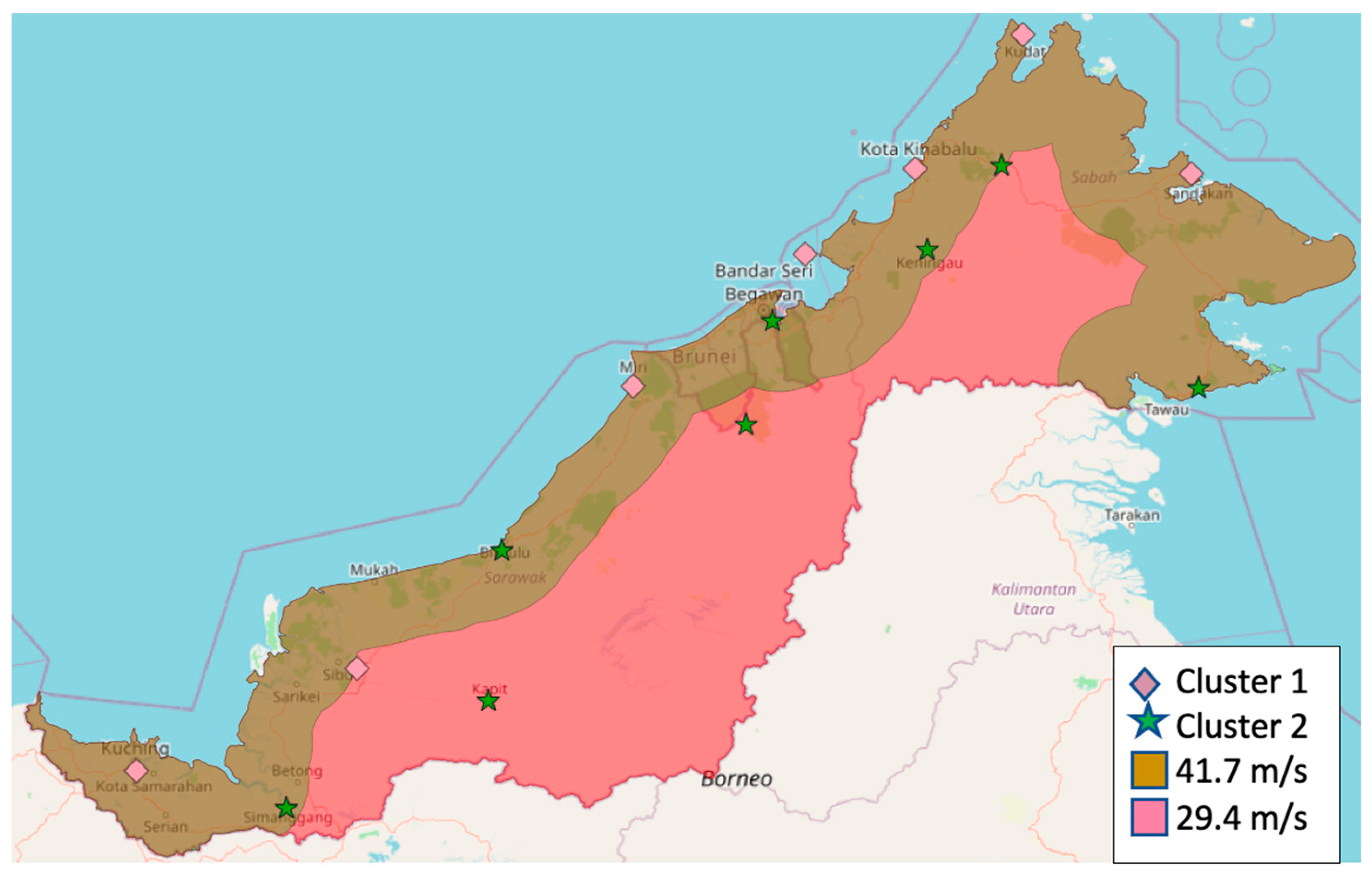
Figure 19 shows suggestions for the basic wind speeds (Vs) distribution map for the Borneo region. The region has been divided into two main areas that tally with the cluster produced by the earlier analysis. The coastal zone consists of Cluster 1 in the majority, a higher wind speed cluster where the highest wind speed recorded is 41.7 m/s. The inland zone is approximately 50 km from the coastline, however, contain the second cluster, which consists of lower speed wind stations. The maximum wind speed for this cluster was 29.4 m/s.
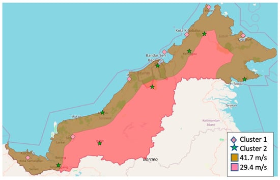
Figure 19.
Clustering map for Borneo.
3.6. Discussion
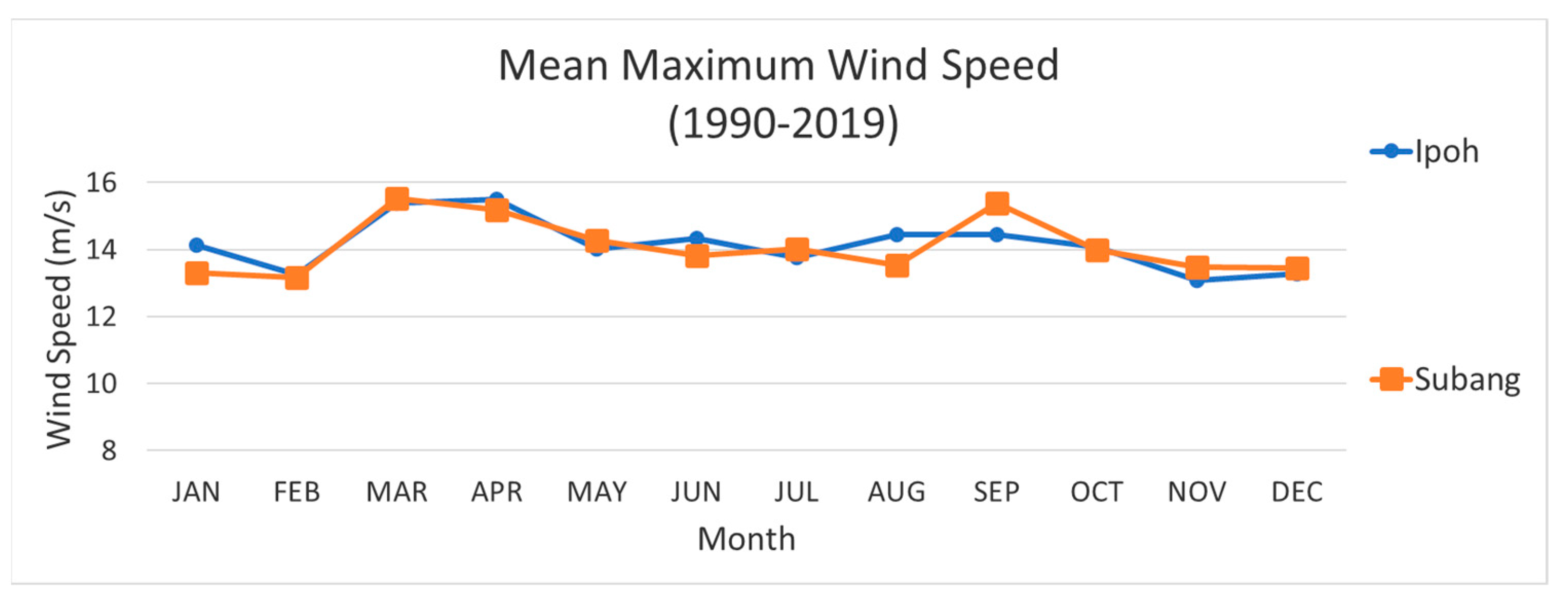
Figure 20 below shows the detailed clustering for each subgroup based on the Wards method. For example, in Cluster 1.a, the cluster contains the station of Ipoh and Subang, where the fluctuation of wind speed happens in February and March. However, both stations are located nearly 170 km away, and the 30 years mean maximum wind speeds are fit to each other. Therefore, it is certain that both areas of wind characteristics are the same.

Figure 20.
Sub-cluster 1.a.
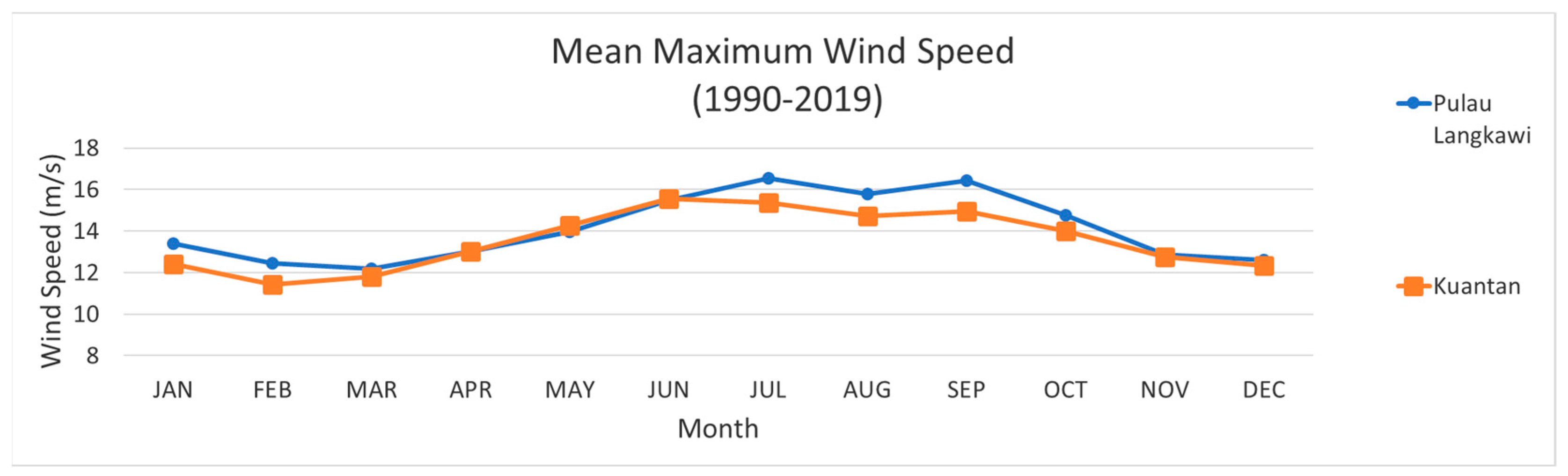
In the sub-cluster 1.e, the wind trends for two of the stations fit each other as shown in Figure 21 below. The mean maximum data show both station trends are the same trend throughout the year. September to February is when the wind started to decrease its speed gradually. The phenomena occurred during transition and the southwest monsoon, where both locations were experiencing heavy downpour. The increase in speed for both stations started in March to September when the southeast monsoon is taken place. The similarity of both geographic conditions is that the Kuantan wind station is located near the South China Sea and Pulau Langkawi wind station is located at Malacca Strait.
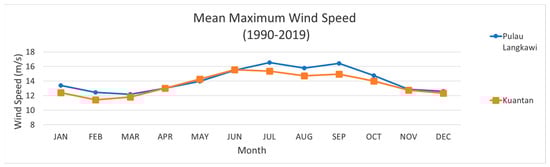
Figure 21.
Sub-cluster 1.e.
Masseran (2012) studied the spatial analysis of wind energy, which came out with a map of wind speed for both West and East Malaysia. The study used the Spatial Prediction method to create a theoretical mean of wind speed for 60 stations involved in this study and then created a map of wind speed for both East and West of Malaysia. However, the Masseran (2012) research focuses on the mean average wind speed, which is lower than the focus of the current research, which uses the highest wind speed. There is a similarity to Masseran’s (2012) research where the mapping for Peninsular Malaysia suggests that the highest wind speed value is located in the northern part of the peninsula, a similar result with the current research where the highest wind speed normally occurs in the northern part of the peninsula. Figure 22 below shows the map of mean wind speed in Peninsular Malaysia [23].

Figure 22.
Map of mean wind speed in Peninsular Malaysia [23].
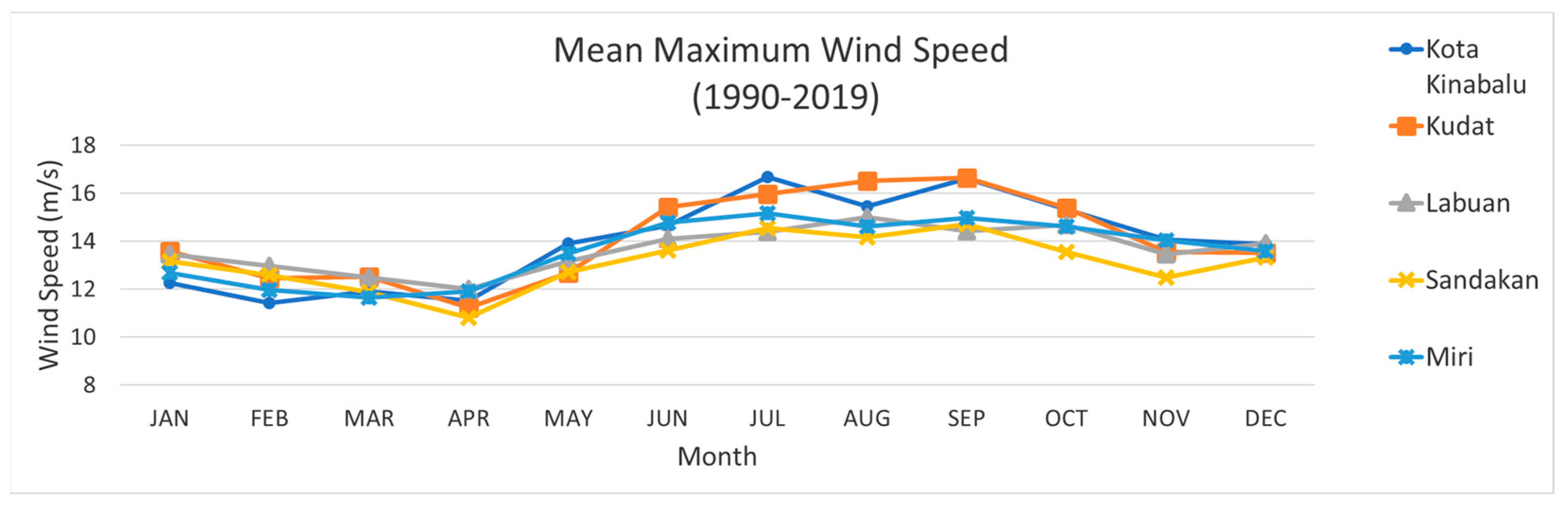
Figure 23 below shows the perfect fit trend for all five wind stations, four of which are located on the east coast of Sabah and one on the northern coast of Sarawak. The trend shows a decreasing speed from September to April due to the northeast monsoon and started to increase in speed from late April to September. The decrease in wind speed for these five stations was a gradual decrease due to the high concentration of moisture during the northeast monsoon. There is a sharp increase in speed during the southwest monsoon, where the failure of the structure is expected to be high due to higher wind speed.
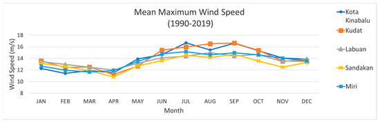
Figure 23.
Sub-cluster 1B.b.
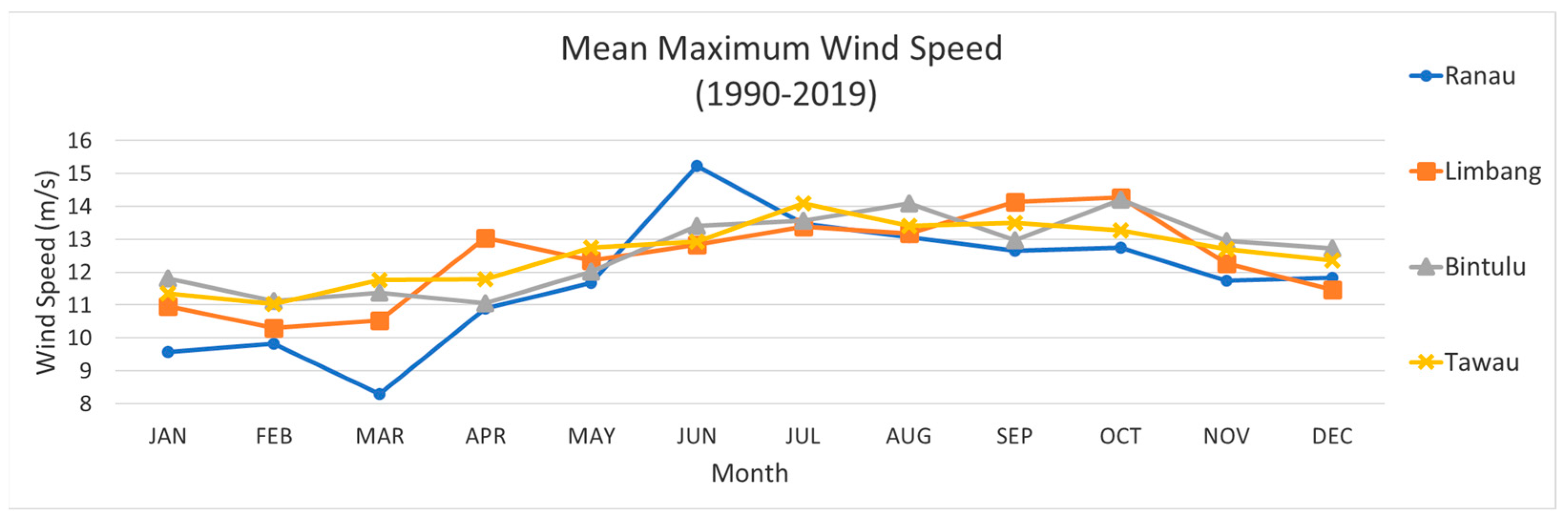
However, the second sub-cluster of the second cluster shows a seasonal trend compared to the first subcluster of Cluster 2 as shown in Figure 24 below. The trend shows a significant decrease in wind speed from November to February due to the raining season. The increase in speed was gradual from March to October. The increase, however, was only around 3 m/s. The effect of the seasonal monsoon for this sub-cluster was because three of the sites were in the coastal area of Sabah and Sarawak, where the researchers found that the location affects the wind speed compared to the inland site where the fluctuation of wind speed is less.

Figure 24.
Sub-cluster 2B.b.
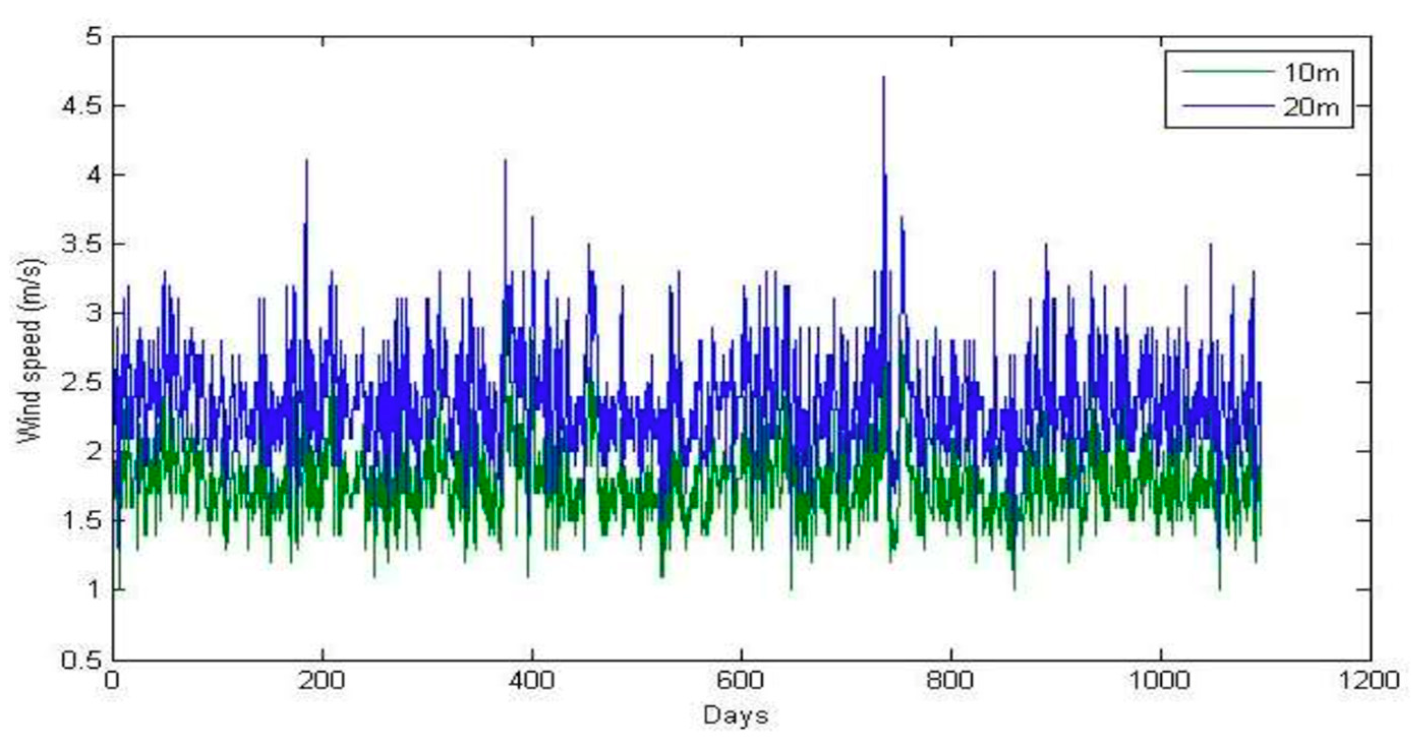
Lawan (2015) also conducted similar observations in Kuching for three years from January 2010 to December 2012. The study’s objective was to see the potential of wind energy in the Kuching area for small-scale power harvesting. One of the findings similar to the current research is the wind speed data, which was obtained every 10 s and averaged every 5 min. The data were then mean by hourly basis and plotted based on two heights, 10 m and 20 m [24]. The plot for the 10 m and 20 m wind speed is tabulated in Figure 25 below.
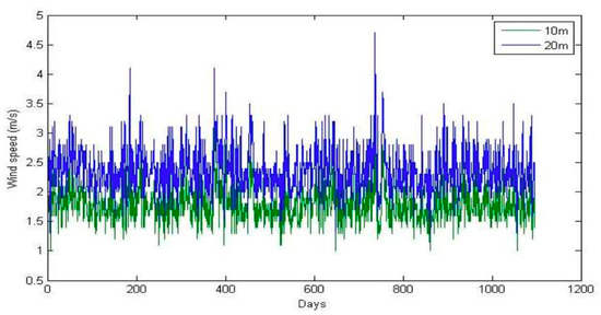
Figure 25.
Variation of wind speed at different altitudes (Lawan et al. 2015) [24].
The plot above shows a similar trend with the current research where the highest wind speed observed in Kuching is within July to September each year for the consistent three years. Therefore, the findings of Lawan in terms of wind trend in Kuching tally with the current research, although the data method was different. Lawan used the monitoring device, and the current research used 95% confidence interval to find the mean monthly data of 30 years of wind speed from the Malaysian Meteorological Department.
Table 7 shows the comparison of findings found in other research that relates to this analysis and result of this paper. The result found that many of the methods used in this paper are similar and give higher accuracy during analysis.
Table 7.
Method and result comparison.
4. Conclusions
From this research, the highest wind speed trend can be plotted as a map. The study observed that 30 years of data were persistent each year with a similar trend found at similar groups each year. The study also found that the highest wind speed in the same cluster tends to be similar. The intensity of the maximum wind speed, however, was dependent on the trend range of the cluster. Therefore, the mapping using the Wards method of clustering is possible and usable for predicting the highest wind speed in the area.
Author Contributions
Writing—original draft, A.A.; Supervision, H.H. All authors have read and agreed to the published version of the manuscript.
Funding
This research received no external funding.
Data Availability Statement
Raw data were generated at Malaysian Meteorological Department wind station. Derived data supporting the findings of this study are available from the Malaysian Meteorological Department (MET) on request.
Conflicts of Interest
The authors declare no conflict of interest.
References
- Liu, Y.X.; Hong, H.P. Estimating Quantiles of Extreme Wind Speed Using Generalized Extreme Value Distribution Fitted Based on the Order Statistics. Wind. Struct. 2022, 34, 469–482. [Google Scholar]
- Ashrafi, A.; Chowdhury, J.; Hangan, H. Comparison of aerodynamic loading of a high-rise building subjected to boundary layer and tornadic winds. Wind. Struct. 2022, 34, 395–405. [Google Scholar]
- Ah, C.J.; Mauricio, G.; Jeffrey, C.; Ellen, M.; Jonathan, C.; Ahmed, E. Structural Performance of an Electricity Tower under Extreme Loading Using the Applied Element Method—A Case Study. Wind. Struct. 2022, 34, 313–319. [Google Scholar]
- Why Clusters Matter. The UK Offshore. 2013. Available online: https://www.offshorewindus.org/wp-content/uploads/2013/08/UK-offshore-wind-supply-chain_why-clusters-matter.pdf (accessed on 15 February 2023).
- Kusiak, A.; Li, W. Short-term prediction of wind power with a clustering approach. Renew. Energy 2010, 35, 2362–2369. [Google Scholar]
- Angosto, J.M.; Elvira-Rendueles, B.; Bayo, J.; Moreno, J.; Vergara, N.; Moreno-Clavel, J.; Moreno-Grau, S. Wind Classification through Cluster Analysis for the Development of Predictive Statistical Models on Atmospheric Pollution. Adv. Air Pollut. 2002, 11, 635–644. [Google Scholar]
- Yesilbudak, M. Clustering Analysis of Multidimensional Wind Speed Data Using K-Means Approach. In Proceedings of the 2016 IEEE International Conference on Renewable Energy Research and Applications, ICRERA, Birmingham, UK, 20–23 November 2016; Volume 5, pp. 961–965. [Google Scholar]
- Van Vuuren, C.Y.J.; Vermeulen, H.J. Clustering of wind resource data for the South African renewable energy development zones. J. Energy South. Afr. 2019, 30, 126–143. [Google Scholar] [CrossRef]
- Clifton, A.; Lundquist, J.K. Data Clustering Reveals Climate Impacts on Local Wind Phenomena. J. Appl. Meteorol. Clim. 2012, 51, 1547–1557. [Google Scholar] [CrossRef]
- Malaysian Communications and Multimedia Commission (MCMC)|Suruhanjaya Komunikasi Dan Multimedia Malaysia (SKMM)—Menara Komunikasi Di Kg. Gelong Badak, Bachok Kelantan Tumbang Akibat Cuaca Buruk. 2021. Available online: https://www.mcmc.gov.my/ms/media/press-releases/menara-komunikasi-di-kg-gelong-badak-bachok-kelant (accessed on 14 February 2023).
- Zuhairi, H.; Hassan, A.; Rahulan, G. Malaysian Standard Code of Practice on Wind Loading for Building Structure. 2002. Available online: https://mysol.jsm.gov.my/getPdfFile/eyJpdiI6ImpzZUdWOEJjNTQ0VzRWVDNCcjZ0Snc9PSIsInZhbHVlIjoidDI0UlF6dFVzWEp0d1lXdWgvVjdkQT09IiwibWFjIjoiZjNiNzBlYzA5ZDc4ZDA0ZGZhMGJlZWJkNDhiYWQ4YTI4ZGE5NGJiZjE3NTc1MjYzNjczZWI2MjQzNmEwZGNlMCJ9 (accessed on 14 February 2023).
- Isyumov, N.; Case, P.; Ho, T.; Soegiarso, R. Wind tunnel model studies to predict the action of wind on the projected 558 m Jakarta Tower. Wind. Struct. 2001, 4, 299–314. [Google Scholar] [CrossRef]
- World Meteorological Organization. Standards and Recommended Practices. 2022. Available online: https://public.wmo.int/en/resources/standards-technical-regulations (accessed on 9 February 2023).
- Tiang, T.L.; Ishak, D. Technical review of wind energy potential as small-scale power generation sources in Penang Island Malaysia. Renew. Sustain. Energy Rev. 2012, 16, 3034–3042. [Google Scholar] [CrossRef]
- Yu, X.; Zhang, W.; Zang, H.; Yang, H. Wind Power Interval Forecasting Based on Confidence Interval Optimization. Energies 2018, 11, 3336. [Google Scholar] [CrossRef]
- Kristina, I.; Zucchi, D.; Znc, H. Lognormal and Normal Distribution. 2021. Available online: https://www.investopedia.com/articles/investing/102014/lognormal-and-normal-distribution.asp (accessed on 1 February 2023).
- Zheng, C.W.; Pan, J.; Li, J.X. Assessing the China Sea wind energy and wave energy resources from 1988 to 2009. Ocean Eng. 2013, 65, 39–48. [Google Scholar] [CrossRef]
- Javed, A.; Lee, B.S.; Rizzo, D.M. A Benchmark Study on Time Series Clustering. Mach. Learn. Appl. 2020, 1, 100001. [Google Scholar] [CrossRef]
- Wu, X.; Kumar, V.; Quinlan, J.R.; Ghosh, J.; Yang, Q.; Motoda, H.; McLachlan, G.J.; Ng, A.; Liu, B.; Yu, P.S.; et al. Top 10 algorithms in data mining. Knowl. Inf. Syst. 2008, 14, 1–37. [Google Scholar] [CrossRef]
- Azizi, E.; Kharrati-Shishavan, H.; Mohammadi-Ivatloo, B.; Shotorbani, A.M. Wind Speed Clustering Using Linkage-Ward Method: A Case Study of Khaaf, Iran. Gazi Univ. J. Sci. 2019, 32, 945–954. [Google Scholar] [CrossRef]
- Sardá-Espinosa, A. Time-Series Clustering in R Using the Dtwclust Package. R J. 2019, 11, 22–43. [Google Scholar] [CrossRef]
- Kok, P.H.; Akhir, M.F.; Tangang, F.T. Thermal frontal zone along the east coast of Peninsular Malaysia. Cont. Shelf Res. 2015, 110, 1–15. [Google Scholar] [CrossRef]
- Masseran, N.; Razali, A.M.; Ibrahim, K.; Zin, W.Z.W.; Zaharim, A. On Spatial Analysis of Wind Energy Potential in Malaysia. WSEAS Trans. Math. 2012, 11, 467–477. [Google Scholar]
- Lawan, S.; Abidin, W.; Chai, W.; Baharun, A.; Masri, T. Wind Energy Potential in Kuching Areas of Sarawak for Small-Scale Power Application. Int. J. Eng. Res. Afr. 2015, 15, 1–10. [Google Scholar] [CrossRef]


Disclaimer/Publisher’s Note: The statements, opinions and data contained in all publications are solely those of the individual author(s) and contributor(s) and not of MDPI and/or the editor(s). MDPI and/or the editor(s) disclaim responsibility for any injury to people or property resulting from any ideas, methods, instructions or products referred to in the content. |
© 2024 by the authors. Licensee MDPI, Basel, Switzerland. This article is an open access article distributed under the terms and conditions of the Creative Commons Attribution (CC BY) license (https://creativecommons.org/licenses/by/4.0/).